
Automatic Detection and Classification of Steel Surface Defect Using Deep Convolutional Neural Networks

1
School of Computer Science and Technology, University of Chinese Academy of Sciences, Beijing 100049, China
2
Shenyang Institute of Computing Technology, Chinese Academy of Sciences, Shenyang 110168, China
*
Author to whom correspondence should be addressed.
Metals 2021, 11(3), 388; https://doi.org/10.3390/met11030388
Submission received: 22 January 2021
/
Revised: 3 February 2021
/
Accepted: 9 February 2021
/
Published: 26 February 2021
(This article belongs to the Special Issue Application of Artificial Neural Networks in Studies of Steels and Alloys)
Abstract
:Automatic detection of steel surface defects is very important for product quality control in the steel industry. However, the traditional method cannot be well applied in the production line, because of its low accuracy and slow running speed. The current, popular algorithm (based on deep learning) also has the problem of low accuracy, and there is still a lot of room for improvement. This paper proposes a method combining improved ResNet50 and enhanced faster region convolutional neural networks (faster R-CNN) to reduce the average running time and improve the accuracy. Firstly, the image input into the improved ResNet50 model, which add the deformable revolution network (DCN) and improved cutout to classify the sample with defects and without defects. If the probability of having a defect is less than 0.3, the algorithm directly outputs the sample without defects. Otherwise, the samples are further input into the improved faster R-CNN, which adds spatial pyramid pooling (SPP), enhanced feature pyramid networks (FPN), and matrix NMS. The final output is the location and classification of the defect in the sample or without defect in the sample. By analyzing the data set obtained in the real factory environment, the accuracy of this method can reach 98.2%. At the same time, the average running time is faster than other models.
1. Introduction
Steel plates are indispensable materials for the automobile industry, national defense industry, machinery manufacturing, chemical industry, light industry, etc. However, due to the problems of raw materials and technology, various types of defects will be produced in the production process of steel plates—especially cracks, scabs, curling edges, cavities, abrasions, and other defects on the surface [1]. These have a fatal impact on the corrosion resistance and strength of the steel plate, and affect the economic benefits of the factory. At present, the surface defect detection of strip steel mostly adopts the method of manual detection. This method is easily affected by the subjective factors of the testing personnel. Moreover, the accuracy of the test results is low, and the reliability is poor. Therefore, it is essential to study the algorithm of automatic real-time detection of surface defects on the production line.
In the past decades, researchers have developed a variety of algorithms to detect defects on steel surfaces [2,3,4,5,6,7,8,9,10,11,12,13,14]. One is the traditional methods is based on statistical information and image features. This method requires researchers to manually design some image features and conduct statistical analysis on these features to obtain the detection results. The commonly used methods are Sobel [15], canny [16], hog [17], local binary patterns (LBP) [18], Fourier transform [19], wavelet transform [20], etc. For instance, Shi et al. [3] propose an improved Sobel algorithm with eight directional templates. It helps to obtain overall edge information, makes edge detection more accurate and faster, and finally makes the algorithm more robust. Liu et al. [4] present different feature extraction approaches (scale invariant feature transform (SIFT), speeded up robust features (SURF) and LBP) and various classifiers (back propagation (BP) neural network, support vector machine (SVM), and extreme learning machine (ELM)) to find the fastest combination method with satisfactory classification accuracy. The method based on machine learning usually extracts some image features first, and then processes these features by a learning algorithm to detect surface defects. Some commonly used algorithms include SVM, artificial neural networks (ANN) [17,18], and Adaboost. Wang et al. [5] propose a novel computational framework, based on SVM and spreading algorithm. The algorithm first uses the SVM algorithm to get the location and shape of the defect, and then uses a spreading algorithm to classify the detected defects. Finally, the covariance matrix is used to calculate the defect size. Kang et al. [6] discuss an approach to detect surface defects of steel strips based on a feed-forward neural network (FFN).
In recent years, with the popularity of computer vision methods based on deep learning [7,8,9,10,11,12,13,14,19,20], more and more researchers have applied deep learning methods to surface defect detection, and replaced the traditional and machine learning methods. This automatic defect detection method is based on deep learning, and can significantly improve product quality and production efficiency, as well as realize end-to-end surface defect detection. This algorithm also can automatically extract the deep and robust features of the image and obtain the results, and complete the task of defect detection efficiently and accurately. At present, the deep learning algorithms used in defect detection mainly include Autoencoder, generative adversarial networks (GAN), and convolutional neural networks (CNN). He et al. [7] propose a semi-supervised learning approach named CAE-SGAN (convolutional autoencoder (CAE) and semi-supervised generative adversarial networks (SGAN)), based on GAN, which improves the performance with limited samples, and Autoencoder, which is used to extract image features. Thomas et al. [8] present an anomaly detection based on deep generative adversarial networks (AnoGAN) to learn a manifold of normal anatomical variability, accompanying a novel anomaly scoring scheme based on the mapping from image space to a latent space. The method based on CNN can be divided into three sub-areas: Image classification [9], image segmentation [10,11], and object detection [12,13,14]. Lee et al. [9] propose a classification method of steel defects based on CNN and class activation maps. It can implement a real-time decision-making process. Tabernik et al. [10] developed an architecture based on image segmentation, which can train the network with fewer samples. This is more suitable for the industrial environment. Surface defect detection algorithms based on object recognition can be divided into two categories: Single-stage and two-stage. Single-stage object recognition algorithms mainly include ‘you only look once’ (YOLO). For example, Li et al. [12] have improved the YOLO algorithm, which contains 27 convolution layers and can provide end-to-end solutions. It can predict the location, size, and category of defects at the same time. Two-stage object recognition algorithms mainly include faster region convolutional neural networks (faster R-CNN) [13]. Firstly, a region proposal is applied to an image to select the region with possible objects, and then the candidate images, which are considered as positive samples in the first step, are taken as sub-image to classify and locate these. Oh et al. [14] advance an approach based on faster R-CNN. They use Inception-ResNet-V2 and data augmentation to improve the accuracy of the model.
As mentioned above, a variety of algorithms have been proposed with the development of machine learning and computer vision, and they all have their own strengths and weaknesses. Traditional and machine learning based methods are usually sensitive to defect scale and noise and are easily affected. Moreover, the accuracy of this algorithm cannot meet the actual needs of automatic defect detection. Some features need to be designed manually, and the scope of the application is very limited. The classification method based on deep learning can only classify images, but cannot determine the location and size of defects. This has a significant impact on the later data analysis. It is very difficult to train a stable and accurate model based on GAN and reinforcement learning. To realize the automatic detection and location of steel plate surface defects, further improve the accuracy and stability, and reduce the average running time of the algorithm. This paper presents a method combining the classification model with the object recognition model. The main contributions of this paper are summarized below.
- Firstly, we propose an improved faster R-CNN model, which can detect multi-scale defects better by adding spatial pyramid pooling (SPP) [21,22,23,24,25], and enhanced feature pyramid networks (FPN) [26] modules. To increase the detection accuracy of crazing defects, we modify the aspect ratio of the anchor. By using the new matrix NMS [27] algorithm, we can get the bounding box faster and better.
- In this paper, we use a combination of the classification model and object detection model, which can significantly improve the accuracy and reduce the average running time of the algorithm.
The organizational structure of this paper is as follows: Section 2 introduces the structure of our algorithm, including the overall architecture, classification model, object detection model, etc. Section 3 analyzes the dataset and guides the improvement of the algorithm. Section 4 and Section 5 use the experiment to prove the accuracy and efficiency of the algorithm, and compare our results with other methods. Finally, Section 5 summarizes the paper and draws a conclusion.
2. Methodology
The core of deep learning ([30], chapter 1) is feature learning, which can acquire multi-level features through the multi-layer network, thus solving the previous problem that requires manual design features. In this paper, a convolution neural network (CNN) ([30], chapter 5) in deep learning is used, which can learn the features of steel surface images by using convolution to detect and locate them. A typical convolution neural network is composed of modules, which are composed of a convolution, pooling, full connection layer, etc. For example, ResNet is made up of convolution layers, residual blocks, and fully connected layers. Because there are very few samples with defects in the actual production environment, it will greatly reduce the average running time of the algorithm to first classify the samples with or without defects through a classifier. Therefore, this paper uses the binary image classification and object detection algorithm at the same time to improve accuracy and reduce average running time.
As shown in Figure 1, first, the image is resized to 224 × 224. Then, the samples are divided into without defect or other through threshold = 0.3 in the classification model improved ResNet50, which add the deformable revolution network (DCN) and improved cutout. If the probability of having a defect is less than 0.3, the algorithm directly outputs the sample without defects. The other samples are resized to 800 × 1344, and further input into the object detection model improved faster R-CNN, which add spatial pyramid pooling (SPP), enhanced feature pyramid networks (FPN), and matrix NMS to detect the defects. The final output is the location and classification of the defect in the sample or without defect in the sample. The following will introduce two parts of the algorithm.
2.1. Classification Model—Improved ResNet50
ResNet [31] is one of the most powerful CNN, which has incomparable performance and has a wide range of uses, including feature extraction as the backbone network and image classification directly. It can be seen in the field of object detection and image segmentation. ResNet network is innovating based on the reference to the VGG19 [32] network. The changes are mainly reflected in the addition of residual units, the use of convolution with stride = 2 for downsampling, and the use of the global average pooling layer to replace the full connection layer. A vital design principle of ResNet is that when the size of the feature map is reduced by half, the number of feature maps is doubled, which keeps the complexity of the network layer. After adding the residual module, which can reduce the degradation of deep CNN in ResNet, we can build a deeper network to achieve better results.
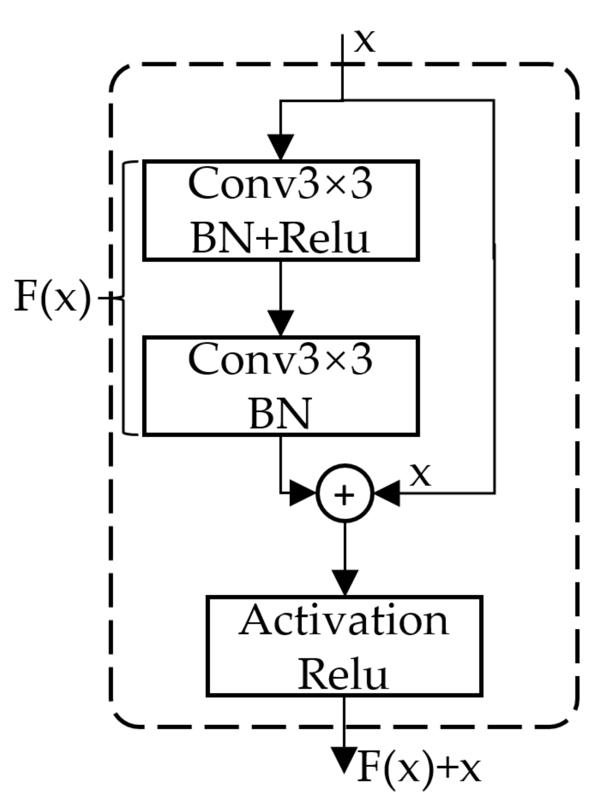
As shown in Figure 2, residual networks become easier to optimize by joining shortcut connections x. Several layers of the neural network containing a shortcut connection are referred to as a residual block. A residual block consists of two paths, one for the normal convolution layers and one for the shortcut connection. Conv3 × 3 represents the convolution operation using the 3 × 3 convolution kernel. BN stands for batch normalization operation. When the input is x, the feature we want to learn is F(x) + x. When the residual is zero, the residual module only performs identity calculation, and the performance will not degrade. In fact, the residual will not be zero, which will make the residual module learn new features based on the input features, so it has better performance.
To improve the performance of ResNet, He et al. [28] proposed an improved method ResNet-vd. As shown in Figure 3, the residual module of ResNet is on the left, and ResNet-vd is on the right. The main improvements are as follows: The downsampling operation of the left half through convolution 1 × 1 with stride = 2 is transferred to the convolution of 3 × 3, the downsampling operation of the right half through convolution 1 × 1 is canceled, and the average pooling layer is added to downsampling the feature map. Through these improvements, the model significantly improves the accuracy and robustness without increasing the amount of computation, and can generate a better feature map. Conv1 × 1 represents the convolution operation using the 1 × 1 convolution kernel. BA represents batch normalization operation and relu activation. B stands for batch normalization operation. Avgpool represents the average pooling layer. Stride is the step size of the convolution operation. Setting it to 2 can reduce the size of the feature. “+” indicates that the feature maps of two paths are added by pixel.
Figure 4 shows the detailed architecture of ResNet50-vd network. The whole network in Figure 4 on the left consists of the stem module, four residual modules, and a fully connected neural network layer. The numbers 32, 64, 256 in the figure represent the number of convolution channels. The stem module is composed of three 3 × 3 convolutions and max pooling, and uses stride = 2 in the first convolution and Max pooling to achieve downsampling. Therefore, the output feature map of the stem module is half the size of the input, and its number of channels is 64. The modules from stage 1 to stage 4 contain one block1 and several block2. It can be seen from Figure 4b that block1 consists of two paths to form a downsampling block. On the left side is a bottleneck structure composed of three convolutions, which are used to learn new features. On the right side is a structure composed of a convolution and AvgPooling, which are used to process the input into the same size and scale as the output of the bottleneck structure. But for stage2 to Stage4, block1 is the same as Figure 3b with the stride = 2 parameter to scale the size of the feature map to half. Block2, like block 1, are composed of two paths. The difference is that the structure on the right side of block 2 is a shortcut connection that forms the residual module with the bottom structure. The size of the output feature map from stem to Stage4 is [7, 14, 28, 56, 112]. The number of convolution channels from stem to Stage4 is [64, 256, 512, 1024, 2048]. Therefore, the final output feature map of Stage4 is 7 × 7 × 2048. The final FC layer of the model uses an average pooling layer and a fully connected layer. The average pooling layer averages the feature map of each channel from 7 × 7 to one value, so we get the feature map of 1 × 1 × 2048 by taking the output of Stage4 as the input. Finally, through a fully connected layer with softmax activation function, which output has two values, which are the probability of whether the image has defects or not.
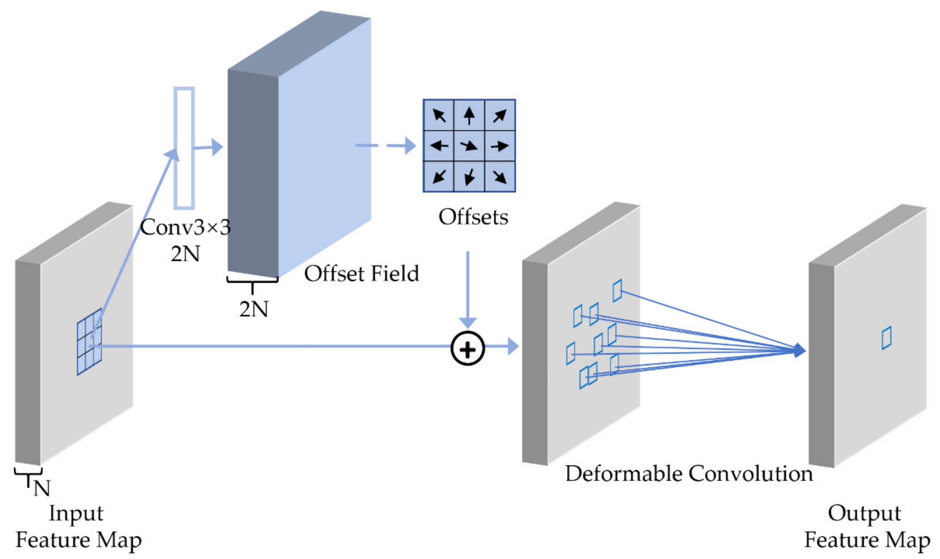
The traditional convolution can’t make adaptive changes when the object is magnified or rotated, due to the defined calculation rules, while the deformable convolution can make adaptive changes by changing the input sampling position. Therefore, dcn-v2 [29] is added to ResNet-vd to increase the adaptability of object deformation. From Figure 5, we can see clearly that deformable convolution uses an additional convolution layer to learn offset. The input feature map and offset are then used together as inputs to the deformable convolution layer. The sample points are shifted by offset first, and then convoluted by the input feature map. In this article, deformable convolution is applied to all 3 × 3 convolution layers from stage 2 to stage 4 of ResNet50-vd. Therefore, there are 13 layers of deformable convolution in the network.
2.2. Object Detection Model—Improved Faster R-CNN
Faster R-CNN [33] is a two-stage object detection algorithm, which consists of three parts: Feature extraction network, region propose network (RPN), and R-CNN. Firstly, it uses feature extraction network to extract the feature map of the image, and then inputs the extracted feature map into RPN to generate the bounding box. Then the generated bounding box is regressed by R-CNN to get a more accurate bounding box, and the images in the box are classified.
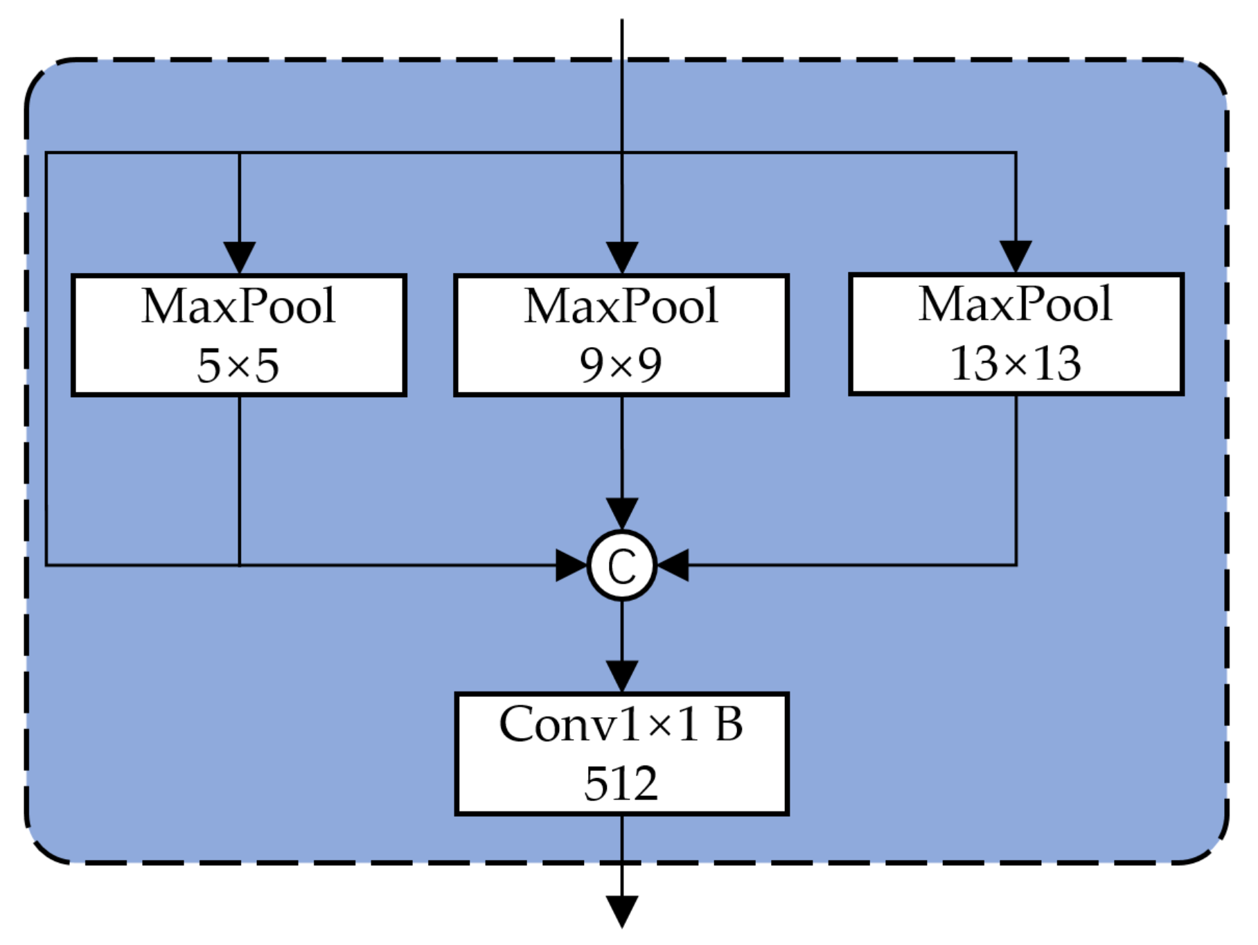
As shown in Figure 6, to increase the detection effect of multi-scale defects, we use ResNet50-vd-dcn, which is the same as the classification network, and delete the last full connection part and FPN as the feature extraction network. At the same time, spatial pyramid pooling (SPP, Figure 7) is added to the Convblock before FPN P1-P5, which can also increase the detection accuracy of defects of different sizes. To improve the effect of the feature extraction network, we further use Coordconv [34] to replace 1 × 1 convolution in FPN. It can improve the efficiency of model training and extract features more accurately.
In the RPN of faster R-CNN, we need non-maximum suppression (NMS) [35] to pick out the best one from the bounding boxes with the same class. The way to achieve this is to eliminate those with lower confidence and IOU higher than a certain threshold for the same class. To solve the problem of overlapping objects in traditional NMS and the low efficiency of serial computation in soft NMS [36], matrix NMS [27] is used in this paper. The overall architecture is shown below.
3. Steel Defect Dataset
The dataset used in this paper comes from the Kaggle competition, “Severstal: Steel Defect Detection” [37], with a total of 12,568 steel sheet grayscale images with the size of 1600 × 256 in the training dataset. Because there is a big gap between the height and width of the original dataset, we divided each image into four images with the size of 400 × 256 in the experiment. Therefore, there are 50,272 samples in our experiment, including 37,080 samples without defects, 12,876 samples with only one type of defect, and 316 samples with two types of defects.
As shown in Figure 8, there are four types of defects in the dataset: Pitted surface, crazing, scrapes, and patches. First, select two images for each class of defects in the dataset. Then, second, mark the bounding box on the picture. Finally, change all the pictures to 256 × 256 and put them on one picture. The classification model uses all the images with defects as one class, and the images without defects as another class, as shown in Table 1. It can be clearly seen from Table 2 that 1306 pictures have pitted surface defects, 214 pictures have inclusion defects, 9980 pictures have scratch defects, 1376 pictures have patch defects, and 316 pictures have two kinds of defects. Images of various defects with bounding box and label used in object detection model are shown in Table 2.
It can be seen from Table 1 and Table 2 that there is a large imbalance in the dataset. In particular, crazing defects only account for 1.6% of the total number of defect samples. Also, the number of no defects samples is too large, accounting for the majority of the total loss, which makes the optimization direction of the model is not what we want. To reduce the impact of imbalanced data sets on the algorithm, firstly, we use the data augmentation method to expand the crazing defect samples to 800 to increase the diversity of samples. Furthermore, the weighted cross entropy loss [38] function and focal loss [39] function are introduced in training.
Let me first introduce the standard cross entropy loss function. The cross entropy describes the distance between two probability distributions, and the closer its value is, the closer the two distributions are. The cross entropy loss function is also the cross entropy between the output of the algorithm and the label. The higher the value is, the more the output is the same as the label, and the higher the accuracy is. Formula (1) is used to calculate the cross entropy loss.
where , , x is the output of the algorithm and y is the actual label.
The idea of weighted cross entropy is to use a coefficient to describe the importance of samples in loss. For a small number of samples, strengthen its contribution to loss, for a large number of samples reduce its contribution to loss. The formula is as follows.
where , there is only a little change between this and cross entropy, that is, a coefficient is added to the discrimination of positive samples. In the object detection task, the weight of each defect is represented by a list . In the classification task, the list is .
Focal loss is improved, based on cross entropy loss. This new loss function can reduce the weight of samples that are easy to classify, and make the model pay more attention to the learning of difficult samples.
where , is the same as in cross entropy loss, and are super parameters. Usually, = 2, = 0.75. is called modulating factor. It can adjust the weight of easy to classify samples, which makes the model pay more attention to learning difficult to classify samples in training.
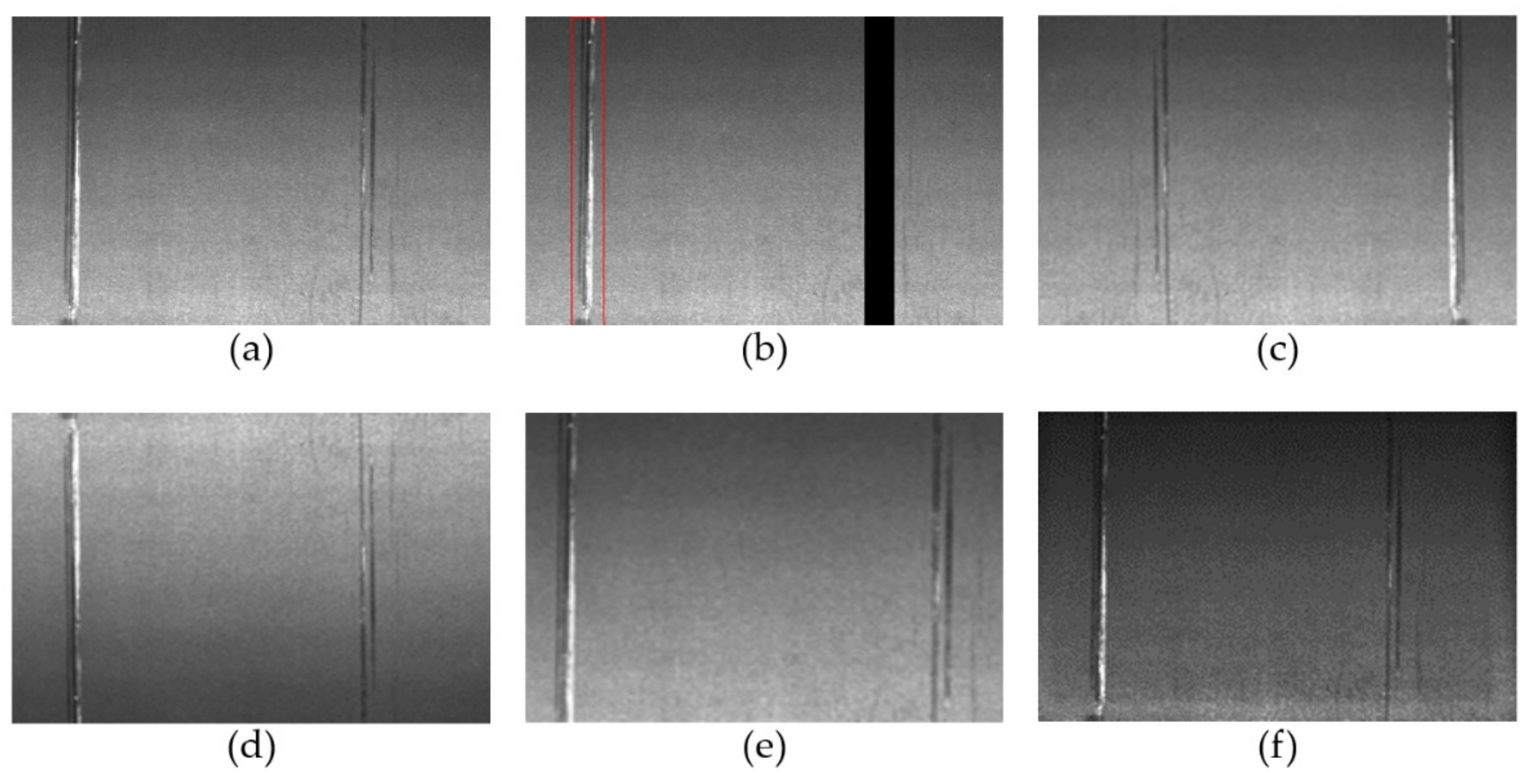
Because training CNN requires a large number of samples, it is difficult to obtain them in the actual production environment. In this paper, data augmentation [40] is used to increase the diversity of samples and improve the accuracy and robustness of the algorithm. By using data augmentation, which is a regularization method, the model reduces overfitting and improves the generalization ability of the network. The methods used in this paper include an improved cutout, horizontal flip, vertical flip, random cropping, and random contrast and brightness transformation. Figure 9 shows the results of various data augmentation methods.
The original cutout method [41] is very simple—that is, randomly delete an area on the image and replace it with zero. In this paper, we study an object detection problem, which includes the label box and class information of four defects. Therefore, we improve the cutout method, randomly delete the label box with a probability of 0.5 and fill it with 0. Only when all the label boxes in a sample are deleted, the label changes to no defect. As shown in Figure 9a,b, there are two scratch defects in the original image. After random improved cutout data augmentation, only one defect is left, and the other defect area is filled with 0. Horizontal and vertical flipping is used in Figure 9c,d, with a probability of 0.5. Random cropping is used in Figure 9e. The top, bottom, left, and right of the image are cropped no more than 15%. After that, the image is resized to 400 × 256. Random contrast and brightness transformation are used in Figure 9f. The probability of 0.5 is used to decide whether to carry out the contrast or brightness transformation. If the two parameters are changed, the transformation range of the image is limited to 50%.
From Figure 8a, we can see that the pitted surface defect is usually small in the steel plate surface defect detection task. We can see from Figure 10 that the defect accounts for a large proportion of the statistical value with a small area. And the area of crazing defect is relatively small. To improve the accuracy of small defect detection, this paper uses SPP and FPN to increase the effect of multi-scale feature extraction.
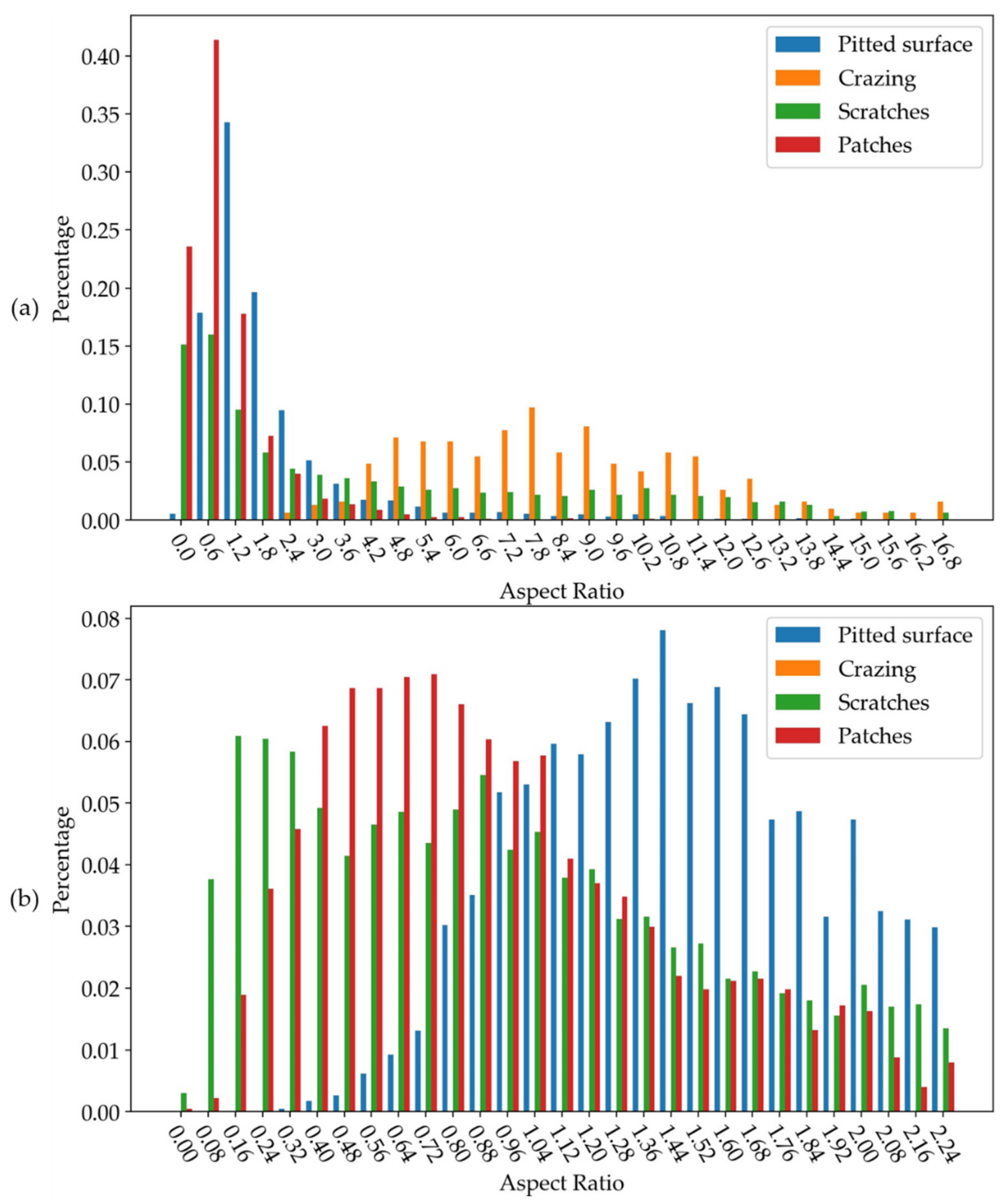
By counting the aspect ratio of various defects, we find a large aspect ratio for cracking and scratches defects, as shown in Figure 11a. Scratch defects also account for a large proportion in a very small proportion, as shown in Figure 11b (b only shows the data in the range of 0–2.4, in more detail). To improve the detection accuracy of these two parts, the anchor setting in faster R-CNN is changed from [0.5, 1, 2.0] to [0.25, 0.5, 1, 2, 5]. By using k-means++ [42] algorithm to cluster bounding box, it is found that this setting can also meet the needs of most defects. The clustering results are shown in Table 3.
4. Training
Due to the small number of samples with defects, transfer learning is used to increase the accuracy and stability of the classification and object detection models. All models are trained with Imagenet data set first, and then the training parameters are used as the initialization parameters of the model used in this paper. As shown in Table 1 and Table 2, we divide the data set into training set with 80% proportion and validation set with 20% proportion.
In this paper, we study the classification model and object detection model. The task of the classification model is to classify samples into those with defects and those without. The task of the object detection model is to identify the location and class of defects in a sample.
In the classification model, to find a more suitable learning rate for this dataset, we use the search method to find the best learning rate in the range of [10−7–10]. The search method is to set a learning rate and then train one epoch to get the loss of the model. The search results are shown in Figure 12. Finally, we chose the learning rate of 0.01. To optimizer the function, we choose Momentum, which has a faster convergence speed and smaller oscillation than the original SGD and momentum = 0.9.
A total of 80 epochs were trained in the model. After training 40 epochs, the learning rate of every 20 epochs is multiplied by 0.5. The loss of the training process is shown in Figure 13. The hardware environment used in the training is AMD Ryzen 5 2600x CPU, 32G DDR4 RAM, and NVIDIA GTX 1080 GPU with 8 GB of video memory. The deep learning framework uses open-source Paddlepaddle, version 2.0. Figure 14 shows the change of accuracy during training. The maximum value is about 0.974.
In the object detection model, we train 50 epochs with a learning rate of 0.0025, batch_size of 4, and warmup of 2500. After training 40 epochs, the learning rate of every five epochs is multiplied by 0.25. To optimizer the function, we choose the same as the classification model Momentum with momentum = 0.9. Data augmentation uses random cropping, horizontal flip, vertical flip, contrast and brightness transformation. Finally, the input image size is changed to 800 × 1344. The hardware environment used in the training is AMD Ryzen 5 2600x CPU, 32G DDR4 RAM, and NVIDIA GTX 1080 GPU. Figure 15 and Figure 16 show the changes of loss and bbox_map during training, respectively. The maximum value of bbox_map was 87.6.
5. Results and Discussion
5.1. Evaluation Metrics
To accurately evaluate the effect of the model, this paper selects recall, precision, F1 score, Accuracy, mean average precision (mAP), and other metrics to compare the model.
Table 4 shows the confusion matrix, in which true positive (TP) means that the positive sample is correctly identified as a positive sample, true negative (TN) means that the negative sample is correctly identified as a negative sample, false positive (FP) means that the negative sample is wrongly identified as a positive sample, and false negative (FN) means that the positive sample is wrongly identified as a negative sample.
Recall is defined, as in formula (4), which indicates the proportion of positive samples in the sample that are correctly identified.
The definition of precision is shown in formula (5), which indicates the proportion of real positive samples among the identified positive samples.
Using recall or precision alone cannot evaluate the performance of the model well. Therefore, the F1 score is introduced to consider recall and precision together. The definition of the F1 score is shown in formula (6).
Accuracy is generally used to evaluate the global accuracy of a model, which cannot contain too much information and cannot comprehensively evaluate the performance of a model. Its definition is shown in formula (7).
AP is the area under the precision-recall curve. Generally speaking, the better a classifier is, the higher the AP value is. mAP is the average of AP of multiple classes. This means that the AP of each class is averaged again, and the value of mAP is obtained. This metric is the most important one in the target detection algorithm.
5.2. The Result of the Classification Model
For the classification algorithm, we compare ResNet and ResNet _ vd, ResNet_ vd_ dcnv2, ResNet_ vd_ dcnv2_ ImprovedCutout, Fadli et al. [43], and konovalenko et al. [44]. We can find that the improved method has better performance, and the highest accuracy can reach 0.9752. By comparison, it is found that the improved convolution block (ResNet_ vd), DCN, and improved cutout methods can increase the accuracy of the model. The last column in Table 5 shows the average run time per image with batch_size = 4. We can see that the accuracy of the model is improved without significantly increasing the running time. For ResNet_vd_dcnV2_ImprovedCutout, it optimizes the data augmentation during training, but only improves the time spent in training the model and improves the accuracy of the model. Because the model’s structure has not changed, it takes the same amount of time to predict as ResNet_vd_dcnV2.
The algorithm uses the test time augmentation (TTA) method in the validation. It can be seen from Table 5 that TTA can increase the accuracy by about 0.05%. Figure 17 shows the confusion matrix of the classification model after TTA. We can see that the classification error rate of the last model is the lowest, whether they are samples that with or without defects. Figure 18 shows the P-R curve and ROC curve of model ResNet_ vd_ dcnv2_ImprovedCutout. We can see that recall and precision of the model have high values at the equilibrium point, which indicates that the model has high accuracy and robustness.
5.3. The Result of Improved Faster R-CNN
Figure 19 shows the result of defect detection by the improved faster R-CNN object detection model. Three defect images of each class are selected in the validation set. First, they are resized to 800 × 1344, and then they are input into the trained faster R-CNN to get the defect detection results. The bounding box with a probability value greater than 0.5 is drawn into the picture, and the detection result picture with a green bounding box is obtained, as shown in the below row of pictures in Figure 19a–e. The bounding box labeled in the original dataset is drawn in blue to the original image, and the images in the upper row are obtained. From (a) to (e) shows the detection results of a pitted surface defect, cracking defect, scrapes defect, patches defect, and multiple defects, respectively. From a, we can see that the model can detect the defect that the real label is not marked. This defect really exists, but it is not obvious. We can clearly see from b that the cracking defect is very slender. By modifying the anchor in faster R-CNN, the detection accuracy of this class is improved. From the middle sample in c, the algorithm detects more defect areas than the labeled bounding box. This also shows a problem that some samples in the original data set are not labeled accurately. The data set will be further processed in future research. From d and e, we can see that the algorithm can detect defects well and determine their categories. In particular, many kinds of defects in e can be detected.
mAP is an important metric to evaluate the object detection model. As shown in Table 6, we used mAP to compare the various models. We can see that the model based on faster R-CNN has higher mAP than the model based on YOLO. The added DCN module can better adapt to various shapes of defects. The FPN and SPP can detect multi-scale defects better, especially the pitted defects, which are smaller and more. The object detection model is also found in the pixel block space, and the output is the bounding box in Cartesian space, so Coordconv is very suitable. Adding Coordconv can improve the AP value of the model as a whole. The mAP of the final model is 0.876, which can accurately detect the surface defects of steel.
5.4. The Result of Our Model
To improve the accuracy and stability of the algorithm and reduce the average running time of processing each image. In this paper, we use a combination of the classification model and object detection model, as shown in Figure 1. First of all, we input the image into the classification model to obtain the defect probability of the sample. If the probability is less than 0.3, we will directly output the sample without defect. In this way, we obtained 7224 samples that were predicted to have no defects. The accuracy of these samples is 0.991, including 7159 samples with correct prediction results and 65 samples with wrong prediction results. Second, the remaining 2830 samples are processed with the object detection model. The final accuracy of these samples is 0.961. This accuracy is lower than that of all samples directly using the detection model, because, after the classification model processing, the remaining samples without defects are more difficult to detect. Finally, it can be seen from Table 7, the accuracy of the classification model and object detection model is analyzed, and the accuracy of the whole model is 0.982.
6. Conclusions
In previous decades, a large number of researchers have participated in the research of steel surface defect detection. Moreover, a variety of algorithms has been proposed with the development of machine learning and computer vision. Traditional and machine learning based methods are usually sensitive to defect scale and noise, and are easily affected. Moreover, the accuracy of this algorithm cannot meet the actual needs of automatic defect detection. Some features need to be designed manually, and the scope of the application is very limited. The classification method based on deep learning can only classify images, but cannot determine the location and size of defects. This has a great impact on the later data analysis. It is very difficult to train a stable and accurate model based on GAN and reinforcement learning. In addition, the method based on object detection has a lot of room for improvement.
To realize the automatic detection and location of steel plate surface defects, further improve the accuracy and stability, and reduce the average running time of the algorithm. In this research, we studied a method that combined a binary classification model and object detection model to reduce the average running time. Through analysis, we found that pitted surface defect is usually small and not obvious, so the accuracy of this class is not high. In the improved faster R-CNN model, by adding FPN and SPP to the feature extraction part of faster R-CNN, the accuracy of this kind of defect is improved. In addition, the accuracy of cracking defect detection is not high because it is narrow and long. The accuracy is improved by changing the default anchor of faster R-CNN. By using the new matrix NMS algorithm, we can get the bounding box faster and better in the final stage of the object detection algorithm. In the improved ResNet50-vd model, which is the backbone of the classification model and object recognition model, by adding the DCN and improved cutout, we can better detect various shapes of defects with higher accuracy and better robustness.
Through the square comparison, we found that this method can be applied to steel surface defect detection with high accuracy. The best result is achieved by combining the classification model improved ResNet, and the object detection model improved aster R-CNN. The accuracy changed from 0.975 for the single classification model and 0.972 for the object detection model to 0.982 for the final model. The average running time of the model is obviously reduced.
Experiments show that there are some problems in the annotation information of datasets. For example, some pitted surface defects are not marked, some areas marked with defects have problems, and some images with defects are put in the samples without defects. Although the annotation information of some samples has been modified, it will be further improved in future research. After processing the data set, the algorithm will be further improved to achieve higher accuracy. Finally, in future research we will study the methods of model compression and acceleration, which can greatly reduce the running time of the algorithm.
Author Contributions
Conceptualization, S.W. and X.X.; methodology, S.W. and X.X.; software, S.W.; validation, S.W.; investigation, S.W.; resources, L.Y. and B.Y.; data curation, S.W.; writing—original draft preparation, S.W.; writing—review and editing, S.W. and X.X.; visualization, L.Y. and B.Y.; supervision, S.W.; project administration, X.X.; funding acquisition, X.X. All authors have read and agreed to the published version of the manuscript.
Funding
This research was funded by Department of science & technology of Liaoning Province, China, grant number XLYC180839.
Institutional Review Board Statement
Not applicable.
Informed Consent Statement
Not applicable.
Data Availability Statement
Publicly available datasets were analyzed in this study. This data can be found here: https://www.kaggle.com/c/severstal-steel-defect-detection/overview (access on 26 July 2019).
Conflicts of Interest
The authors declare no conflict of interest.
Nomenclature
| ANN | Artificial neural networks |
| BP | Back Propagation |
| CAE | Convolutional Autoencoder |
| CNN | Convolutional Neural Networks |
| DCN | Deformable revolution network |
| ELM | Extreme Learning Machine |
| Faster R-CNN | Faster Region Convolutional Neural Networks |
| FFN | Feed-forward neural network |
| FPN | Feature pyramid networks |
| GAN | Generative Adversarial Networks |
| LBP | Local Binary Patterns |
| NMS | Non-Maximum Suppression |
| RPN | Region propose network |
| SGAN | Semi-supervised Generative Adversarial Networks |
| SIFT | Scale Invariant Feature Transform |
| SPP | Spatial Pyramid Pooling |
| SURF | Speeded Up Robust Features |
| SVM | Support Vector Machine |
| TTA | Test time augmentation |
| YOLO | You only look once |
| super parameters | |
| cross entropy loss | |
| weighted cross entropy loss | |
| Focal loss |
References
- Luo, Q.; Fang, X.; Liu, L.; Yang, C.; Sun, Y. Automated Visual Defect Detection for Flat Steel Surface: A Survey. IEEE Trans. Instrum. Meas. 2020, 69, 626–644. [Google Scholar] [CrossRef] [Green Version]
- Thomas, G.B.; Jenkins, M.S.; Mahapatra, R.B. Investigation of strand surface defects using mould instrumentation and modelling. Ironmak. Steelmak. 2004, 31, 485–494. [Google Scholar] [CrossRef]
- Shi, T.; Kong, J.; Wang, X.; Liu, Z.; Zheng, G. Improved Sobel algorithm for defect detection of rail surfaces with enhanced efficiency and accuracy. J. Cent. South Univ. 2016, 23, 2867–2875. [Google Scholar] [CrossRef]
- Liu, Y.; Xu, K.; Wang, D. Online Surface Defect Identification of Cold Rolled Strips Based on Local Binary Pattern and Extreme Learning Machine. Metals 2018, 8, 197. [Google Scholar] [CrossRef] [Green Version]
- Wang, Z.; Zhu, D. An accurate detection method for surface defects of complex components based on support vector machine and spreading algorithm. Measurement 2019, 147, 106886. [Google Scholar] [CrossRef]
- Kang, G.; Liu, H. Surface defects inspection of cold rolled strips based on neural network. In Proceedings of the 2005 International Conference on Machine Learning and Cybernetics(ICMLC 2005), Guangzhou, China, 18–21 August 2005; pp. 5034–5037. [Google Scholar]
- Di, H.; Ke, X.; Peng, Z.; Zhou, D. Surface defect classification of steels with a new semi-supervised learning method. Opt. Laser. Eng. 2019, 117, 40–48. [Google Scholar] [CrossRef]
- Schlegl, T.; Seeböck, P.; Waldstein, S.M.; Schmidt-Erfurth, U.; Langs, G. Unsupervised Anomaly Detection with Generative Adversarial Networks to Guide Marker Discovery. In Proceedings of the 25th International Conference on Information Processing in Medical Imaging (IPMI 2017), Boone, NC, USA, 25–30 June 2017; pp. 146–157. [Google Scholar]
- Lee, S.Y.; Tama, B.A.; Moon, S.J.; Lee, S. Steel Surface Defect Diagnostics Using Deep Convolutional Neural Network and Class Activation Map. Appl. Sci. 2019, 9, 5449. [Google Scholar] [CrossRef] [Green Version]
- Tabernik, D.; Šela, S.; Skvarč, J.; Skočaj, D. Segmentation-based deep-learning approach for surface-defect detection. J. Intell. Manuf. 2020, 31, 759–776. [Google Scholar] [CrossRef] [Green Version]
- Prappacher, N.; Bullmann, M.; Bohn, G.; Deinzer, F.; Linke, A. Defect Detection on Rolling Element Surface Scans Using Neural Image Segmentation. Appl. Sci. 2020, 10, 3290. [Google Scholar] [CrossRef]
- Li, J.; Su, Z.; Geng, J.; Yin, Y. Real-time Detection of Steel Strip Surface Defects Based on Improved YOLO Detection Network. IFAC PapersOnLine 2018, 51, 76–81. [Google Scholar] [CrossRef]
- Wei, R.; Song, Y.; Zhang, Y. Enhanced Faster Region Convolutional Neural Networks for Steel Surface Defect Detection. ISIJ Int. 2020, 60, 539–545. [Google Scholar] [CrossRef] [Green Version]
- Oh, S.-J.; Jung, M.-J.; Lim, C.; Shin, S.-C. Automatic Detection of Welding Defects Using Faster R-CNN. Appl. Sci. 2020, 10, 8629. [Google Scholar] [CrossRef]
- Borselli, A.; Colla, V.; Vannucci, M.; Veroli, M. A fuzzy inference system applied to defect detection in flat steel production. In Proceedings of the 2010 IEEE International Conference on Fuzzy Systems (FUZZ-IEEE 2010), Barcelona, Spain, 18–23 July 2010; pp. 1–6. [Google Scholar]
- Tang, B.; Kong, J.; Wang, X.; Chen, L. Surface Inspection System of Steel Strip Based on Machine Vision. In Proceedings of the 2009 First International Workshop on Database Technology and Applications, Wuhan, China, 25–26 April 2009; pp. 359–362. [Google Scholar]
- Wang, Y.; Xia, H.; Yuan, X.; Li, L.; Sun, B. Distributed defect recognition on steel surfaces using an improved random forest algorithm with optimal multi-feature-set fusion. Multimed. Tools Appl. 2018, 77, 16741–16770. [Google Scholar] [CrossRef]
- Liu, Y.; Xu, K.; Xu, J. An Improved MB-LBP Defect Recognition Approach for the Surface of Steel Plates. Appl. Sci. 2019, 9, 4222. [Google Scholar] [CrossRef] [Green Version]
- Aiger, D.; Talbot, H. The phase only transform for unsupervised surface defect detection. In Proceedings of the 2010 IEEE Conference on Computer Vision and Pattern Recognition (CVPR 2010), San Francisco, CA, USA, 13–18 June 2010; pp. 295–302. [Google Scholar]
- Liu, W.; Yan, Y. Automated surface defect detection for cold-rolled steel strip based on wavelet anisotropic diffusion method. Int. J. Ind. Syst. Eng. 2014, 17, 224–239. [Google Scholar] [CrossRef]
- Mikołajczyk, T.; Nowicki, K.; Kłodowski, A.; Pimenov, D.Y. Neural network approach for automatic image analysis of cutting edge wear. Mech. Syst. Signal. Process. 2017, 88, 100–110. [Google Scholar] [CrossRef]
- Mikołajczyk, T.; Nowicki, K.; Bustillo, A.; Pimenov, D.Y. Predicting tool life in turning operations using neural networks and image processing. Mech. Syst. Signal. Process. 2018, 104, 503–513. [Google Scholar] [CrossRef]
- Lim, W.; Jang, D.; Lee, T. Speech emotion recognition using convolutional and recurrent neural networks. In Proceedings of the 2016 Asia-Pacific Signal and Information Processing Association Annual Summit and Conference (APSIPA), Jeju, Korea, 13–15 December 2016; pp. 1–4. [Google Scholar]
- Abueidda, D.W.; Koric, S.; Sobh, N.A.; Sehitoglu, H. Deep learning for plasticity and thermo-viscoplasticity. Int. J. Plasticity 2021, 136, 102852. [Google Scholar] [CrossRef]
- He, K.; Zhang, X.; Ren, S.; Sun, J. Spatial Pyramid Pooling in Deep Convolutional Networks for Visual Recognition. IEEE Trans. Pattern Anal. Mach. Intell. 2015, 37, 1904–1916. [Google Scholar] [CrossRef] [PubMed] [Green Version]
- Lin, T.; Dollár, P.; Girshick, R.; He, K.; Hariharan, B.; Belongie, S. Feature Pyramid Networks for Object Detection. In Proceedings of the 2017 IEEE Conference on Computer Vision and Pattern Recognition (CVPR 2017), Honolulu, HI, USA, 21–26 July 2017; pp. 936–944. [Google Scholar]
- Wang, X.; Zhang, R.; Kong, T.; Li, L.; Shen, C. SOLOv2: Dynamic and Fast Instance Segmentation. In Proceedings of the Thirty-Fourth Conference on Neural Information Processing Systems (NeurIPS 2020), Vancouver, BC, Canada, 6–12 December 2020. [Google Scholar]
- He, T.; Zhang, Z.; Zhang, H.; Zhang, Z.; Xie, J.; Li, M. Bag of Tricks for Image Classification with Convolutional Neural Networks. In Proceedings of the 2019 IEEE/CVF Conference on Computer Vision and Pattern Recognition (CVPR 2019), Long Beach, CA, USA, 15–20 June 2019; pp. 558–567. [Google Scholar]
- Zhu, X.; Hu, H.; Lin, S.; Dai, J. Deformable ConvNets V2: More Deformable, Better Results. In Proceedings of the 2019 IEEE/CVF Conference on Computer Vision and Pattern Recognition (CVPR 2019), Long Beach, CA, USA, 15–20 June 2019; pp. 9300–9308. [Google Scholar]
- Chollet, F. Deep Learning with Python; Manning Publications Co.: Shelter Island, NY, USA, 2018. [Google Scholar]
- He, K.; Zhang, X.; Ren, S.; Sun, J. Deep residual learning for image recognition. In Proceedings of the 2016 IEEE Conference on Computer Vision and Pattern Recognition (CVPR 2016), Las Vegas, NV, USA, 27–30 June 2016; pp. 770–778. [Google Scholar]
- Simonyan, K.; Zisserman, A. Very deep convolutional networks for large-scale image recognition. In Proceedings of the 3rd International Conference on Learning Representations (ICLR 2015), San Diego, CA, USA, 7–9 May 2015. [Google Scholar]
- Ren, S.; He, K.; Girshick, R.; Sun, J. Faster R-CNN: Towards Real-Time Object Detection with Region Proposal Networks. IEEE Trans. Pattern Anal. Mach. Intell. 2016, 39, 1137–1149. [Google Scholar] [CrossRef] [Green Version]
- Liu, R.; Lehman, J.; Molino, P.; Such, F.P.; Frank, E.; Sergeev, A.; Yosinski, J. An Intriguing Failing of Convolutional Neural Networks and the CoordConv Solution. In Proceedings of the 32nd Conference on Neural Information Processing Systems (NeurIPS 2018), Montréal, QC, Canada, 3–8 December 2018; pp. 9628–9639. [Google Scholar]
- Neubeck, A.; Van Gool, L. Efficient non-maximum suppression. In Proceedings of the 18th International Conference on Pattern Recognition (ICPR 2006), Hong Kong, China, 20–24 August 2006; pp. 850–855. [Google Scholar]
- Bodla, N.; Singh, B.; Chellappa, R.; Davis, L.S. Soft-NMS—Improving Object Detection with One Line of Code. In Proceedings of the 2017 International Conference on Computer Vision (ICCV 2017), Venice, Italy, 22–29 October 2017; pp. 5561–5569. [Google Scholar]
- Severstal: Steel Defect Detection. Available online: https://www.kaggle.com/c/severstal-steel-defect-detection (accessed on 25 June 2020).
- Cai, Z.; Fan, Q.; Feris, R.S.; Vasconcelos, N. A unified multi-scale deep convolutional neural network for fast object detection. In Proceedings of the 14th European Conference on Computer Vision (ECCV 2016), Amsterdam, The Netherlands, 11–14 October 2016; pp. 354–370. [Google Scholar]
- Lin, T.; Goyal, P.; Girshick, R.; He, K.; Dollár, P. Focal Loss for Dense Object Detection. IEEE Trans. Pattern Anal. Mach. Intell. 2020, 42, 318–327. [Google Scholar] [CrossRef] [PubMed] [Green Version]
- Shorten, C.; Khoshgoftaar, T.M. A survey on Image Data Augmentation for Deep Learning. J. Big Data 2019, 6, 1–48. [Google Scholar] [CrossRef]
- DeVries, T.; Taylor, G.W. Improved regularization of convolutional neural networks with cutout. arXiv 2017, arXiv:1708.04552. [Google Scholar]
- Arthur, D.; Vassilvitskii, S. k-means++: The advantages of careful seeding. In Proceedings of the Eighteenth Annual ACM-SIAM Symposium on Discrete Algorithms, New Orleans, LA, USA, 7–9 January 2007; pp. 1027–1035. [Google Scholar]
- Fadli, V.F.; Herlistiono, I.O. Steel Surface Defect Detection using Deep Learning. Int. J. Innov. Sci. Res. Technol. 2020, 5, 244–250. [Google Scholar] [CrossRef]
- Konovalenko, I.; Maruschak, P.; Brezinová, J.; Viňáš, J.; Brezina, J. Steel Surface Defect Classification Using Deep Residual Neural Network. Metals 2020, 10, 846. [Google Scholar] [CrossRef]
Figure 1.
Algorithm Framework.

Figure 2.
Residual block.

Figure 3.
Comparison of ResNet and ResNet-vd. (a) ResNet residual block, (b) ResNet-vd residual block.
Figure 3.
Comparison of ResNet and ResNet-vd. (a) ResNet residual block, (b) ResNet-vd residual block.

Figure 4.
The architecture of ResNet-50-vd. (a) Stem block; (b) Stage1-Block1; (c) Stage1-Block2; (d) FC-Block.
Figure 4.
The architecture of ResNet-50-vd. (a) Stem block; (b) Stage1-Block1; (c) Stage1-Block2; (d) FC-Block.

Figure 5.
Deformable convolution network.

Figure 6.
The architecture of enhanced faster R-CNN.

Figure 7.
Spatial pyramid pooling (SPP).

Figure 8.
Examples of various types surface defect. (a) Pitted surface; (b) crazing; (c) scratches; (d) patches; (e) no defect.
Figure 8.
Examples of various types surface defect. (a) Pitted surface; (b) crazing; (c) scratches; (d) patches; (e) no defect.

Figure 9.
Data augmentation. (a) Original image; (b) improved cutout; (c) horizontal flip; (d) vertical flip; (e) random crop; (f) random contrast and brightness transformation.
Figure 9.
Data augmentation. (a) Original image; (b) improved cutout; (c) horizontal flip; (d) vertical flip; (e) random crop; (f) random contrast and brightness transformation.

Figure 10.
Statistical results of area size of various defects.

Figure 11.
Statistical results for the ratio of height to width of various defects. (a) aspect ratio of various defects; (b) data in (a) in the range of 0–2.4, in more detail.
Figure 11.
Statistical results for the ratio of height to width of various defects. (a) aspect ratio of various defects; (b) data in (a) in the range of 0–2.4, in more detail.

Figure 12.
Find learning rate (Lr).

Figure 13.
Loss of the classification model.

Figure 14.
Accuracy of the classification model.

Figure 15.
Loss of object detection model.

Figure 16.
Bbox_map of object detection model.

Figure 17.
Confusion matrix of the classification model after test time augmentation (TTA). (a) ResNet (b) ResNet-vd (c) ResNet-vcd-dcnV2 (d) ResNet-vd-dcnV2-ImprovedCutout.
Figure 17.
Confusion matrix of the classification model after test time augmentation (TTA). (a) ResNet (b) ResNet-vd (c) ResNet-vcd-dcnV2 (d) ResNet-vd-dcnV2-ImprovedCutout.

Figure 18.
The result of ResNet_ vd_ dcnv2_ Improvedcutout. (a) P-R Curve; (b) ROC Curve.

Figure 19.
Detection results. (a) Pitted surface defect; (b) crazing defect; (c) scratches defect; (d) patches defect; (e) multiple defects.
Figure 19.
Detection results. (a) Pitted surface defect; (b) crazing defect; (c) scratches defect; (d) patches defect; (e) multiple defects.


Table 1.
Classification model dataset.
| Class | Train | Valid | Total |
|---|---|---|---|
| With Defects | 10,553 | 2639 | 13,192 |
| Without Defects | 29,664 | 7416 | 37,080 |
| Total | 40,217 | 10,055 | 50,272 |
Table 2.
Object detection model dataset.
| Class | Train | Valid | Total |
|---|---|---|---|
| Pitted surface | 1044 | 262 | 1306 |
| Crazing | 171 | 43 | 214 |
| Scratches | 7984 | 1996 | 9980 |
| Patches | 1100 | 276 | 1376 |
| Multi Class Defect | 252 | 64 | 316 |
| Without Defect | 29,664 | 7416 | 37,080 |
| Total | 40,215 | 10,057 | 50,272 |
Table 3.
Cluster anchor using k-means++ algorithm.
| 1 | 2 | 3 | 4 | 5 | 6 | 7 | 8 | 9 | 10 | 11 | 12 | 13 | 14 | 15 | 16 | 17 | 18 | 19 | 20 | 21 | 22 | 23 | 24 | 25 | |
|---|---|---|---|---|---|---|---|---|---|---|---|---|---|---|---|---|---|---|---|---|---|---|---|---|---|
| Height | 34 | 436 | 134 | 252 | 38 | 72 | 510 | 512 | 320 | 62 | 172 | 106 | 510 | 82 | 246 | 136 | 510 | 74 | 190 | 508 | 252 | 114 | 504 | 144 | 312 |
| Width | 9 | 9 | 18 | 20 | 23 | 23 | 23 | 31 | 32 | 35 | 35 | 36 | 45 | 58 | 58 | 70 | 73 | 108 | 119 | 142 | 218 | 219 | 294 | 511 | 512 |
Table 4.
Confusion matrix.
| True Class | Predicted Class | |
|---|---|---|
| Positives | Negatives | |
| Positives | TP | FN |
| Negatives | FP | TN |
Table 5.
Comparison of the classification models.
| Model | Original Image | Horizontal Flip | Vertical Flip | TTA | Running Time | ||||
|---|---|---|---|---|---|---|---|---|---|
| F1 | Acc | F1 | Acc | F1 | Acc | F1 | Acc | ||
| Fadli et al. [37] | -- | 0.94 | -- | -- | -- | -- | -- | -- | |
| ResNet | 0.968 | 0.969 | 0.9627 | 0.9628 | 0.9626 | 0.9627 | 0.9673 | 0.9675 | 2.40 ms |
| Konovalenko et al. [38] | -- | 0.9691 | -- | -- | -- | -- | -- | -- | |
| ResNet_vd | 0.9707 | 0.9708 | 0.9694 | 0.9695 | 0.9689 | 0.9690 | 0.9710 | 0.9711 | 2.44 ms |
| ResNet_vd_dcnV2 | 0.9732 | 0.9732 | 0.9726 | 0.9726 | 0.9730 | 0.9731 | 0.9739 | 0.9739 | 2.9 ms |
| ResNet_vd_dcnV2_ImprovedCutout | 0.9747 | 0.9747 | 0.9744 | 0.9744 | 0.9745 | 0.9745 | 0.9752 | 0.9752 | 2.9 ms |
Table 6.
The AP of each type of defect and the total mAP of the model.
| Model | Type of Defect | mAP | |||
|---|---|---|---|---|---|
| Pitted Surface | Crazing | Scratches | Patches | ||
| YOLOv3 | 0.700 | 0.643 | 0.749 | 0.724 | 0.704 |
| Faster-RCNN | 0.801 | 0.767 | 0.874 | 0.865 | 0.827 |
| Faster-RCNN + DCN | 0.806 | 0.782 | 0.881 | 0.876 | 0.836 |
| Faster-RCNN + DCN + FPN&SPP | 0.840 | 0.818 | 0.902 | 0.895 | 0.864 |
| Faster-RCNN + DCN + FPN&SPP + Coordconv | 0.845 | 0.829 | 0.913 | 0.916 | 0.876 |
Table 7.
Comparison of model accuracy and average running time.
| Model | Accuracy | Average Running Time |
|---|---|---|
| Improved ResNet50 | 0.9752 | 2.9 ms |
| Wei et al. [8] | 0.97 | 209.4 ms |
| Improved Faster R-CNN | 0.972 | 214.5 ms |
| Classification and object detection | 0.982 | 63.3 ms |
Publisher’s Note: MDPI stays neutral with regard to jurisdictional claims in published maps and institutional affiliations. |
© 2021 by the authors. Licensee MDPI, Basel, Switzerland. This article is an open access article distributed under the terms and conditions of the Creative Commons Attribution (CC BY) license (http://creativecommons.org/licenses/by/4.0/).
Share and Cite
MDPI and ACS Style
Wang, S.; Xia, X.; Ye, L.; Yang, B. Automatic Detection and Classification of Steel Surface Defect Using Deep Convolutional Neural Networks. Metals 2021, 11, 388. https://doi.org/10.3390/met11030388
AMA Style
Wang S, Xia X, Ye L, Yang B. Automatic Detection and Classification of Steel Surface Defect Using Deep Convolutional Neural Networks. Metals. 2021; 11(3):388. https://doi.org/10.3390/met11030388
Chicago/Turabian StyleWang, Shuai, Xiaojun Xia, Lanqing Ye, and Binbin Yang. 2021. "Automatic Detection and Classification of Steel Surface Defect Using Deep Convolutional Neural Networks" Metals 11, no. 3: 388. https://doi.org/10.3390/met11030388
Note that from the first issue of 2016, this journal uses article numbers instead of page numbers. See further details here.