
Dirlik and Tovo-Benasciutti Spectral Methods in Vibration Fatigue: A Review with a Historical Perspective


1
Dirlik Controls Ltd., 12 Main Street, Rugby CV22 7NP, UK
2
Department of Engineering, University of Ferrara, Via Saragat 1, 44122 Ferrara, Italy
*
Authors to whom correspondence should be addressed.
Metals 2021, 11(9), 1333; https://doi.org/10.3390/met11091333
Submission received: 3 August 2021
/
Revised: 19 August 2021
/
Accepted: 20 August 2021
/
Published: 24 August 2021
(This article belongs to the Special Issue Fracture, Fatigue, and Structural Integrity of Metallic Materials and Components Undergoing Random or Variable Amplitude Loadings)
Abstract
:The frequency domain techniques (also known as “spectral methods”) prove significantly more efficient than the time domain fatigue life calculations, especially when they are used in conjunction with finite element analysis. Frequency domain methods are now well established, and suitable commercial software is commonly available. Among the existing techniques, the methods by Dirlik and by Tovo–Benasciutti (TB) have become the most used. This study presents the historical background and the motivation behind the development of these two spectral methods, by also emphasizing their application and possible limitations. It further presents a brief review of the other spectral methods available for cycle counting directly from the power spectral density of the random loading. Finally, some ideas for future work are suggested.
1. Introduction
The estimation of fatigue life under variable amplitude or random loadings has been an active research topic in the last fifty years, and the activity has further increased in the last two decades. Cumulative damage calculations, in particular, occupy a dominant sector in the structural integrity assessment of metallic components and structures subjected to random fatigue loadings. In order to achieve a high level of structural reliability, fatigue life calculations must be made at several stages of the design and development process. An important aspect of the development of fatigue-resistant components and structures is the ability to estimate component fatigue life and, thus, prevent unexpected failures.
The traditional approach to fatigue analysis—often referred to as “time domain approach”—uses a technique called rainflow cycle counting to decompose a variable amplitude time signal of stress into fatigue cycles [1,2]. The damage from each cycle is then computed using an S/N curve, which characterizes the material strength for constant amplitude loadings. The damage over the entire time signal is finally calculated by summing the damage from all the individual cycles, using, for example, the celebrated Palmgren–Miner linear damage rule. This simple rule, which sums the damage of cycles, regardless of their order in the loading, also postulates that fatigue failure occurs when the damage exceeds a critical level equal to unity [3].
The time domain approach does not present any particular theoretical complexity and, nowadays, it is easy to implement by considering, for example, that the rainflow algorithm is available in some numerical packages [4,5]. The approach may, however, require a long computation time when it has to analyze a lot of digitalized signals of long duration, such as those computed in hundreds of thousands of nodes in a finite element model. This unfortunate circumstance could render the fatigue damage computation the bottleneck of the whole design process.
In addition, the procedure by which stress signals are obtained plays an important role. In fact, the computation time may increase if the random stress signals are obtained by a transient simulation in time domain, which is orders of magnitude slower than an analysis in frequency domain, able to compute harmonic transfer functions and stress power spectral densities with much less computational effort.
For linear systems, fatigue life calculations conducted entirely in the frequency domain can shorten the computation time considerably. This corresponds to the so-called “frequency domain approach” in vibration fatigue. Fatigue life calculation methods based on frequency domain information of a random loading are now well established, and suitable commercial software is commonly available (e.g., nCode DesignLife, Simulia Fe-safe, CAEfatigue, Ansys Random Vibration Fatigue). Among frequency domain methods, one should also number those approaches in which spectral methods are combined with crack growth models with the aim to estimate fatigue life under random loadings [6,7,8,9,10]. Crack growth models, though relevant for the fatigue durability field, are not included in the following discussion, which is concerned with S/N based approaches in frequency domain.
Since the early works of Miles [11] and Bendat [12], and in particular in the past thirty years, tens of spectral methods have been developed and their number continues to rise even today (a short list is found in [13,14]).
However, among all the existing methods, two of them have gained an increased popularity and large use in the scientific and technical community: they are the Dirlik method [15] and the Tovo–Benasciutti (or TB) method [16,17]. One reason for their popularity is their accuracy, often superior to other methods, as highlighted by several comparative studies that are commented on in the following sections.
Among the multitude of spectral methods, the Dirlik and TB methods are specifically considered hereafter as they were invented by the two authors of this paper, who thus have a vantage point in explaining the motivation behind the development of both methods, meanwhile emphasizing some of their theoretical peculiarities. The purpose of this paper is also to comment on their progresses and possible shortcomings, as well as to discuss their relationship with a few other spectral methods, providing some insights into future work. To this regard, this paper is not meant to be, in the strict sense, either a critical review or a comparison of lots of spectral methods; rather, its aim is to focus on the Dirlik and TB methods while also casting a glance on how they interrelate with other existing methods.
2. Random Processes in Frequency Domain: Spectral Properties and Fatigue Damage
2.1. Spectral Properties
Fatigue life assessment is critical in the design of components and structures exposed to random loads, such as a car on a rough road or a wind turbine. These loads can be viewed as the realization of a stationary random process , which can be described in the frequency domain by a power spectral density (PSD) function , where is the circular frequency (in rad/s). The PSD is related to the Fourier transform of [18]. It provides a picture of the energy content of over frequencies. The power spectrum is often used to describe signals for qualification tests [19]. Note that two definitions of PSD exist, namely single-sided versus double-sided. Each one can be function of circular frequency (rad/s) or frequency (Hertz). is a single-sided PSD function of .
It is customary to classify a random signal based on its frequency content, that is, on the shape of its PSD. The signal is said to be “narrow band” if has a peak around a single frequency, generally the resonant frequency of a vibrating system. In all other cases in which the PSD covers a wider range of frequencies, the random signal is not narrow band, and it is named as “wide band” (or “broad band”). Sometimes, more specific definitions (“bimodal”, “trimodal”, “multimodal”, etc.) are adopted to specify that a PSD has two, three, or more well-defined peaks.
Figure 1 compares three time history samples belonging to three types of random processes. The figure emphasizes quite well the differences among the various time histories based on their corresponding PSD, although it considers power spectra with rectangular blocks that are only idealizations of the smoother spectra normally encountered in practical applications.
The definitions of narrow band or wide band process introduced so far are merely qualitative. A more quantitative definition is provided by means of several types of spectral parameters, which are indeed introduced with the purpose of establishing to which degree a random signal is narrow band or wide band. The first parameters are the spectral moments [18]:
The theory shows [18] that, for a random loading with zero mean value, the spectral moment of order zero coincides with the variance of the random signal, ; the root mean square (rms) value is .
Other spectral moments of higher order—or, better, their combinations—are also used to characterize some statistical properties of the random signal that are of interest in fatigue analysis. For example, for a Gaussian process, (rad/s) is the expected number of mean value upcrossings per unit time, while (rad/s) is the expected number of peaks per unit time [18]. For what follows, it is useful to introduce the “mean frequency” (rad/s) of the spectral density; it may be interpreted as the distance of the centroid of the spectral mass from the frequency original [20].
Besides the previous parameters, other quantities, known as bandwidth parameters, are used extensively. They are combinations of spectral moments. Various equivalent definitions exist, but those most used are [18]:
They belong to a more general class, . Note the relationship with the Vanmarcke’s spectral parameter [20]. Both and approach unity for a narrow band process, whilst they approach zero when the spectral width increases. Parameter is related to the definition and properties of the envelope of the random process, and it is often called “groupness parameter” in ocean engineering. Parameter is often called the “irregularity factor”, which is a useful parameter characterizing the behavior of the process. In time domain, the irregularity factor is defined as the ratio of the number of mean value upcrossings to the expected number of peaks , that is ; for a Gaussian process it takes the form , which coincides with . This parameter lies between zero and unity. It approaches unity for a narrow band process in which peaks and troughs are placed symmetrically above and below the mean value of the process. It approaches zero when the process has many peaks between two successive crossings of its mean value.
2.2. Fatigue Damage
The fatigue damage of a random time history of time length is computed in two stages. In the first, a counting method (e.g., rainflow) is applied to , with the purpose of identifying the set of fatigue cycles [2]. Counted cycles have, in general, different amplitudes and mean values, and thus they contribute with a different damage. Therefore, in the second stage, the damage of every counted cycle is summed up to determine the damage of as a whole. This step calls for a damage accumulation rule, as the Palmgren–Miner linear law [3]:
This summation extends over the total number of cycles counted in ; numbers the cycles with amplitude , which would cause a failure after repetitions in a constant amplitude test.
Often, the relationship between stress amplitude and cycles to failure is expressed by a straight line in a log–log diagram, through the S/N curve . This equation is fitted to experimental data by regression analysis. In some cases, a two-slope equation is preferred when it fits experiments better.
In Palmgren–Miner rule, fatigue failure is predicted to occur when damage reaches a critical value equal to unity, even though lower values are recommended in some design codes (e.g., [21]) to account for experimental evidence.
The summation in Equation (3) assumes that the cycles counted in are grouped into bins of cycles, all having the same amplitude . The actual values of and obviously depend on the actual course of . If the instantaneous values of vary randomly—that is, is modeled as a random process—it follows that and are both random variables. In this case, the summation in Equation (3) needs to be reformulated in a probabilistic way:
Here, is the probability distribution of the amplitudes of rainflow cycles, is the number of rainflow cycles counted in , and is the number of cycles to failure at constant amplitude . Notice that the previous expression is very general, as is not restricted to a straight-line equation.
Although, at first glance, the previous formula may appear complicated, it is nothing more than the Palmgren–Miner rule in Equation (3) extended to continuously distributed amplitudes.
Equation (4) can be solved in closed form if one knows the analytical expressions of . This circumstance occurs, for example, when is a narrow band process. In this case, peaks and valleys are placed symmetrically around the mean value of , and each cycle is formed by pairing each peak to the adjacent valley (this corresponds to the peak counting method)—the range is the peak–valley distance. Consequently, each cycle has zero mean and amplitude coincident with the peak value, which in a narrow band process follows a Rayleigh distribution [18]. In a narrow band process, the number of cycles counted is also known, it being equal to the number of crossings of the mean value, . When inserted into Equation (4), the previous mathematical conditions yield the expression of the “narrow band” damage in time interval [18]:
in which is the gamma function. This expression is usually credited to Miles [11] or Bendat [12]. It is restricted to a straight S/N line. In case the S/N relationship is not straight, it is possible to solve Equation (4) numerically, by taking as a Rayleigh distribution.
When the random process is no longer narrow band, the previous formula becomes too conservative. Indeed, in a wide band process, fatigue cycles cannot simply be obtained by joining a peak with a symmetric valley, as is done in the peak counting [2]; actually, this counting procedure would yield cycles with amplitudes larger than those identified by the rainflow counting. On the other hand, the algorithm of the rainflow counting is so intricate that it seems not possible to determine, in closed form, the expression of the probability distribution of amplitudes and mean values of rainflow cycles, and to relate it to the bandwidth parameters of the wide band process.
For this reason, historically, the approach followed initially—easy but oversimplified—was to introduce a correction factor less than unity, by which to reduce the narrow band damage in Equation (5). The correction factor must become smaller and smaller when the spectral bandwidth of the random process becomes wider and wider. Since this inverse relationship is not known, and it cannot be determined in closed form because of the same reasons mentioned above for the rainflow counting, the only feasible way was to calibrate the damage correction factor based on simulation results. The difficult task was to select which bandwidth parameters must enter the correction factor. Assumptions were made based on the trends observed in simulations.
Among the spectral methods that followed this approach, the first, and probably the most famous, one is that of Wirsching and Light, proposed in 1980 [22], in which the correction factor is made to depend solely on the spectral parameter . In subsequent years, other methods following the same idea were proposed. In those methods, the expression of the correction factors was refined by introducing the dependency on other bandwidth parameters. For example, an approach named the “empirical -method” proposed a correction factor in the form [17].
It should come as no surprise that the use of a correction factor for estimating the damage of a wide band process, no matter how simple, has the drawback of not providing the amplitude probability distribution of the cycles causing that damage. Knowing indeed has several advantages. First, it makes it possible to compute the fatigue damage not only for a straight S/N line, but also for any smooth curve with continuous change of slope, with or without endurance limit. Second, the amplitude distribution allows one to determine the cumulative (or loading) spectra of rainflow cycles, and to extrapolate it towards cycles with large amplitudes (rare events).
3. Dirlik Method (1985)
This method can, for sure, be numbered as a milestone among spectral methods. This is testified by the number of citations, to date more than 600 in Google Scholar [23].
As already said, a power spectral density function specifies how the characteristics of a random signal are distributed over a given frequency range. This information is needed in many engineering sectors; techniques to calculate the PSD from a time record are readily available in the form of fast Fourier transform (FFT).
Early in the development of the Dirlik method, because of the complexity of the rainflow counting algorithm, it was decided that it would be such a difficult task to derive in closed form the distribution of rainflow cycles from the PSD function . A Monte Carlo approach was thus employed to generate a sample stress history from using FFT methods [24,25]. Then, the rainflow algorithm was used on to extract the cycles and the probability density function of rainflow counted ranges, which in turn allowed calculating the fatigue damage for any given material constants in an S/N curve.
The idea of the Monte Carlo approach is based on the “weak law of large numbers”, which states that the sample average converges in probability towards the expected value if the sample size increases [26]. It is then important that, in numerical simulations, the sample stress histories are sufficiently long to contain a large number of turning points (peaks and troughs); in fact, the longer the time history, the more chance of catching rare events.
The exact procedure of the approach linking PSDs to rainflow range probability densities is explained fully in [15,27], and it is briefly summarized here.
A total of 70 PSDs of various shapes were considered, some rectangular and some smoothly varying, as shown in Figure 2. To make the comparison easier, power spectra were normalized so that all had the same rms value and the same expected rate of peaks (that is, the same number of rainflow cycles counted in a time interval). With these two parameters kept fixed, the irregularity factor was made to vary (from 0.16 to 0.99) by adjusting the parameters defining the power spectrum shape—which in turn corresponds to varying the spectral moments of order zero, two, and four (, , ).
The rectangular bimodal spectrum (see Figure 2a) was used extensively because of its simplicity to assume a wide range of values of the irregularity factor , having the same rms value and the same expected rate of peaks , by adjusting the amplitudes and the frequency boundaries of the power spectrum.
In preliminary simulation trials, it was, however, observed that the mean frequency of the spectrum (that is, its first order moment ) also has a role in changing the fatigue damage of a simulated time history. To investigate this relationship more closely, 42 out of 70 power spectra were shaped so as to have the same , , , but different . Because the expected rate of peaks is identical for all spectra, a “normalized mean frequency” was introduced:
For a given power spectral density, sample stress time histories were generated using the inverse FFT (IFFT). A single generated stress time history had 1024 points. The simulation procedure was repeated 20 times in order to obtain a sufficiently long record of stress time history. This long record (called one block) consisted of 1024 × 20 = 20,480 time points [15]. The number of 1024 FFT points was not a choice, but it was dictated by the maximum size of the memory and disk capacity of computers available at that time. The use of 20 replicated stress time histories had the very purpose of increasing the entire length of the simulated block. Processed in time domain, the block was converted into a sequence of peaks and troughs, from which fatigue cycles were extracted by means of the rainflow counting and the simple-range counting (which pairs a peak with the next valley [2]). From the set of counted cycles, the probability distributions of simple ranges and rainflow ranges were finally calculated. An example is displayed in Figure 3.
Thanks to the simulation results, it was argued that the probability density function (PDF) of rainflow ranges is to be a mixture of three distributions: an exponential function, a Rayleigh function with variable parameter, and a standard Rayleigh function. The full expression in terms of a normalized variable is [15]:
where is the rainflow range. The coefficients , , and are defined as
where is the normalized mean frequency in Equation (6).
Note that the symbols in Equations (7) and (8) conform to the notation used nowadays, which differs from that originally used in [15]. The quantities , , , and are “best fit” parameters that turned out after minimizing the difference between the observed probability distribution and the analytical one.
The probability distribution in Equation (7) represents the link between the rainflow counted ranges and the power spectral density. The importance of this equation lies in the fact that, once it is used to determine the PDF of rainflow ranges, the life estimation can be made with any form of S/N data by using Equation (4). The use of this method is not restricted to a straight line representation of S/N data on a log–log scale only, which instead could be a smooth curve with continuous change of slope with or without endurance limit. In the case of single slope S/N line, , the substitution of into Equation (4) returns a closed-form expression for the damage in time interval [17,28]:
That described so far is the original version Dirlik method commonly used. A temperature-modified version was also proposed in [29,30,31] to estimate the high-cycle fatigue damage for uniaxial loadings caused by random vibrations directly from a power spectral analysis. The model combines the frequency-based method and the temperature effect, and it is verified by comparison with experimental test results for a high-pressure die-cast aluminum alloy. Actually, the approach in [29] incorporates the temperature effect into the Dirlik method by considering a temperature-dependent inverse slope and fatigue strength and , and by also taking the temperature time history into consideration by using a weighted sum of the damage at each temperature. In this way, the temperature-dependent spectral approach, though developed in [29] only for the Dirlik method, is in fact applicable to any other spectral method, provided that temperature-dependent S/N parameters are used.
4. Tovo–Benasciutti (TB) Method (2002, 2005)
The theory of this method was first laid out in [32]. It postulates that the amplitude–mean joint probability distribution of rainflow cycles lies between two limit distributions, and can be estimated as their linear combination:
Here, is a weight factor that needs to be determined. Unlike Dirlik method, the TB method provides the joint distribution of amplitudes and mean values of rainflow cycles. The two functions and represent the amplitude–mean distributions of the level-crossing counting (LCC) and of the simple-range counting (RC)—actually, the latter is only approximated. Their analytical expressions, not reported here, can be found in [16,32]. The two distributions are shown in Figure 4. Note that involves two Dirac delta functions.
Equation (10) shows that the LCC and RC distributions represent two bounds between which the rainflow cycle distribution is enclosed. In other words, Equation (10) postulates that the rainflow cycle distribution of any random process lies between two limit distributions, and its actual shape depends on the value of .
Likewise in Equation (10), the same weighted sum holds also for the marginal probability distributions , , , and, most importantly, for the damage values:
The latter inequality takes advantage of the fact that and that the simple-range counting damage is approximated as [16,17]. Though, from a practical point of view, the quantity can be interpreted as a correction factor of the narrow band damage, the above arguments clearly demonstrate that the origin of this factor is in fact quite different, and the TB method has a sound theoretical basis.
Turning back now to the weighted sum that links probability distributions and damage values through , the next step to complete the definition of the TB method was to find a proper expression for . At least theoretically, parameter is a function of the whole set of spectral and bandwidth parameters of the PSD of the random process.
Nevertheless, it was—as it seems even today—rather hard, if not impossible, to demonstrate theoretically which spectral parameters contribute to the definition of . Some trends can be argued. In the narrow band case, for example, the rainflow distribution must converge to the Rayleigh one (i.e., LCC function), which in turn requires that for a narrow band process in which and both approach unity. Other trends emerged from numerical simulations. The approach was to generate stress time histories, as in the procedure described for the Dirlik method.
Using simulation results with power spectra densities of various shapes, a first expression was proposed in [32]:
This formula is yet not continuous. Moreover, its accuracy tends to diminish if and differ significantly [13], as in the special case of a lightly damped linear oscillator driven by white noise, whose response has but (irregular process) [18].
From a broader perspective, conflicting views seem to emerge in the literature regarding the accuracy of parameter . While the agreement with simulation results was judged as “excellent” in [32], a less flattering opinion—moreover consistent with the results of [33]—is given in [34], where the use of this formulation of is indeed discouraged.
Apart from this, long before the above studies, it was soon discovered that Equation (12) could be ameliorated by seeking better solutions. Although a first attempt was made in [35] to find a continuous but equally accurate expression to replace Equation (12), it was only in [36], and later in [16], that the expression of used today has finally been developed:
This expression is a result of a best fitting on simulation results from power spectral densities of various shapes (see Figure 5). Similar to the Dirlik method, this formula assumes that the rainflow probability distribution is linked to four spectral moments, , , , and . The soundness of this correlation, first foreseen by Dirlik, was confirmed after comparing frequency domain estimations with time domain simulation results. It was shown in [16] that the use of Equation (13) along with Equation (11) guarantees an excellent accuracy.
After that, this accuracy was further confirmed by other studies (e.g., [33,37]), and the TB method rapidly became popular and widely used, similar to the Dirlik method—though the latter seems to remain the method preferred by most scholars.
Soon after [16] was published, a further attempt was made in [17] to correlate to fractional order spectral moments and (in bandwidth parameter ) by the formula
This choice was suggested after having observed that fractional spectral moments were considered also by other spectral methods (Zhao-Baker [38], “single-moment” [39,40], “empirical -method” [17]). Against all odds, the comparison made in [17] even revealed that the accuracy of Equation (14) is slightly better than Equation (13); however, despite this outcome, quite surprisingly, Equation (14) has been ignored by scholars in favor of Equation (13).
5. Area of Application of Spectral Methods
Since their early development, but especially from the appearance of Dirlik approach in 1985, spectral methods have found ever more application in many engineering fields, even those much different from each other. Over the years, many examples and case studies have been developed in engineering sectors such as automotive, wind, offshore, and marine, not to mention the field of aerospace and advanced composite materials.
Obviously, as already pointed out for spectral methods, here it is also not possible (as well not very useful) to enumerate all the examples or case studies cited in the literature, by also considering that probably a great many of them were not published as scientific articles. Nor is the aim of this section to present a summary list of articles. Rather, the lines that follow have the only purpose of casting a glance at a few representative applications of spectral methods, with special interest on examples that analyze real structures, often with the aid of finite element simulation.
It has indeed to be pointed out that one of the main advantages of spectral methods (which may in fact explain their widespread use) is the possibility to use them in conjunction with computer-aided analysis. Typically, once a finite element model is built and subjected to a known random acceleration/load expressed by a power spectral density, the stress power spectra in each node are calculated and then input directly in a spectral method, which then provides a damage value in each node of the model. If the nodal stress is multiaxial (i.e., a PSD matrix is defined), a multiaxial criterion must be used [41].
Among those existing, multiaxial spectral methods that transform a multiaxial stress into an equivalent uniaxial stress permit the “traditional” spectral methods (like as Dirlik, TB method or others) to be used [42]. This synergistic combination of multiaxial criteria and frequency domain methods has allowed the field of application of spectral methods to be expanded considerably.
In the automotive field, application of spectral methods generally relies on results of multibody and/or finite element simulation at various levels of modeling detail (chassis, engine, tires, etc.) [43,44,45,46,47]. Sometimes the focus is on a specific component—structural or not—that has to endure random vibrations due to road roughness. Interesting is, for example, the study in [48], which applies spectral methods for estimating the road-induced fatigue damage in a carbon steel coil spring based on acceleration signals acquired in a car driving on various road types [48]. A similar goal is pursued in [49], where field measurements and finite element modeling are used for analyzing a structural component of an automotive headlight. The capabilities of spectral methods as design tool are further demonstrated in [50] by an experimental/numerical analysis of a wheel of an industrial vehicle. When computation time becomes essential, it is possible to integrate spectral methods in an algorithm for monitoring fatigue damage in real time using onboard equipment, as demonstrated by the example in [51] with a heavy-duty truck frame.
In the field of maritime engineering, where there are different types of structures subjected to random waves (e.g., ships, mooring systems, offshore wind turbines, and fixed offshore structures), the use of spectral methods is particularly effective. An advantage is that the power spectra for certain sea states (e.g., JONSWAP, Pierson–Moskowitz) are known in closed form and can be input directly in a finite element analysis aimed at determining the structural dynamic behavior and stress response. Frequency-based fatigue analysis methods are also mentioned in design guidelines [52].
An example of frequency domain fatigue analysis of a semi-submersible platform is described in [53]. The study applies spectral methods with multiaxial fatigue criteria to the output of a three-dimensional finite element model. The case study also serves as a basis to compare the accuracy of various spectral methods.
When data storage and computational cost in recording and processing stress time histories are important, spectral methods prove to be particularly advantageous. For example, [54] proposed a structural monitoring system for a ship hull in which a damage detection algorithm using spectral methods is embedded into a wireless sensor.
For offshore wind turbines, the combined effect of wave and wind loadings acting simultaneously is investigated in [55]; the contribution of different sea and/or wind states can also be taken into account. Spectral methods are also used for estimating the structural integrity of welded joints, which constitute a typical structural detail in offshore structures [55,56].
Examples specific to the field of wind engineering show how spectral methods can be used to predict the fatigue damage of wind-excited structures [57,58]; corrections factors are introduced to account for non-Gaussian effects in the output stress caused by nonlinear aerodynamic damping. A spectral based fatigue analysis, integrated with finite element simulation, is the basis for a structural integrity assessment of two welded joints in a wind turbine tubular tower subjected to different wind speed and direction conditions [59]. When a best balance is required between accuracy and overall computation cost, the study suggests the use of the frequency domain approach over the time-domain one—and among spectral methods, TB and Dirlik methods are recommended [59].
The literature also offers examples of use of spectral methods in engineering sectors such as aerospace and electronics, or with composite materials. In the former cases, for example, spectral methods combined with finite element analysis are employed for the virtual qualification of electronic assemblies subjected to aerospace vibratory environment [60]. Other examples with electronic devices [61,62] are discussed in the following section. Concerning composite materials, spectral based approaches attempt to reformulate strength criteria for composite materials (e.g., Tsai–Hill [63], residual strength, or stiffness model [64,65]) to extend their validity to the frequency domain for the case of random vibrations [66]. Even for metal/composite assemblies undergoing random vibrations, an example demonstrates how to combine finite element analysis with spectral methods successfully [67]. Another application is described in [68] for carbon fiber-reinforced silicon carbide ceramic matrix composite, which are considered as excellent materials for thermal protection structures of launch vehicles and spacecraft structures and, for this reason, exposed to thermo-acoustic vibration loading in service.
6. Comparison of Spectral Methods
Although the discussion so far has focused on Dirlik and TB approaches, it should not be forgotten that, in the literature, a great many other spectral methods exist for wide band random processes. They are nevertheless too numerous to list them all here. The following list, certainly not exhaustive, mentions in chronological order those spectral methods that seem to be among the most cited in the literature:
- Wirsching and Light (1980) [22].
- Ortiz and Chen (1987) [72].
- Zhao and Baker (1992) [38].
- Steinberg three-band method (2000) [73].
- Empirical method (2006) [17].
- Gao and Moan (2008) [37].
- Lalanne (2009) [76].
All these frequency domain methods are usually derived for stationary Gaussian processes, but extensions to stationary non-Gaussian processes or to specific subclasses of nonstationary processes (e.g., switching case) have also been proposed. Except for the narrow band case, all these methods are approximate; they differ in what they estimate. While some methods estimate only the expected fatigue damage, others also attempt to also estimate the probability distribution of rainflow amplitudes [17]. Some methods in the previous list (e.g., “single-moment”, Fu–Cebon method and its modified version, Gao and Moan) were developed for bimodal or trimodal processes, and they are now considered as a safe technique to assess the vibration fatigue life of real engineering structures.
With the increase in the number of spectral methods, the need has come to establish which of them is “the best” method. A lot of articles published over the last decades have proposed systematic comparisons among spectral methods, and therefore this work does not repeat such a similar analysis. Rather, it summarizes the main findings from other articles. Readers are advised to draw their own conclusions as to which method is “the best” for their own application after investigating each method’s assumptions, limitations, and application areas. When interpreting the outcomes of comparison studies, an important aspect to consider is the length of simulated time histories, which should be the longest possible so as to increases the chance of observing large amplitude cycles that appear only occasionally, and thus to make the comparison more reliable.
6.1. Comparison between Dirlik and TB Method
Before comparing these two methods with others, it is useful to give them a closer inspection. To this end, this section compares the Dirlik and TB methods for some selected power spectral densities. The comparison considers not only the amplitude probability distribution, but also the “damage distribution” (to be defined below) and the estimated damage. The purpose is to show that, even though the methods yield, in general, very close predictions, some differences may sometimes occur in their amplitude distributions.
The following discussion deals with the power spectral density in Figure 2a, which is defined by the area ratio and by frequencies , , , . The frequency ratios and can be chosen so as to have different [15] or equal [39,40] values. The condition ensures the same spectral bandwidth for both blocks. In this case, the power spectrum is only defined by ratio of areas and frequencies . This type of power spectrum is particularly advantageous, as it allows not only bimodal cases, but also narrow band and band-limited power spectra to be obtained by a suitable choice of geometric parameters. When (whatever ) the spectrum becomes unimodal—whether narrow band or wide band depends on . A small value (e.g., ) assures that each rectangle is narrow band. As increases, the spectrum width widens. Additionally, for this power spectrum, it is easy to obtain closed-form expressions that express , , in terms of , , (see [13]). With such formulae, parameters and can be varied so as to obtained prescribed values of and .
A short list of PSD geometrical and spectral parameters is summarized in Table 1. For every spectrum, the lowest frequency is adjusted so that all power spectra have the same number of peaks per second . The three columns on the right provide the damage ratio for three values of S/N slope.
Among the examples of Table 1, two specific cases are investigated in more detail in Figure 6 and Figure 7. They refer to combinations: , (with , ) and , (with , ). In Figure 6 and Figure 7, the graphs on the left show the amplitude probability distributions and , whereas the graphs on the right show each distribution multiplied by . In all figures, the Rayleigh distribution, also multiplied by on the right graph, is shown for comparison. Values and of the S/N curve are chosen.
The graphs on the right, so suitably devised, have the purpose of highlighting the distribution of the damage contributed by each amplitude. In fact, apart from constant , the quantity is the damage caused by the cycle with amplitude . Looking at this kind of “probability distribution weighted with damage” or simply “damage distribution”, it is possible to explain why, in spite of having different rainflow amplitude distributions, Dirlik and TB methods estimate almost identical damage values. For the example in Figure 6, the damage ratio is , while it slightly grows to for the example in Figure 7. The comparison also demonstrates, at least for the two cases considered in the figures, that a difference in amplitude distributions in the region of small amplitudes is not of concern, since small amplitudes contribute very little to the total damage, especially for high . Furthermore, the graph also makes apparent how the Rayleigh probability distribution always leads to a larger damage.
6.2. Comparison among Spectral Methods (Numerical Simulations)
To our knowledge, one of the earliest comparisons of spectral methods is that performed in [28]—obviously, it does not include the TB method that appeared only about ten years later. The comparison in [28] indicated the Dirlik method as superior to other spectral methods (as, for example, Wirsching‒Light and “single-moment”) for a wide combination of power spectral densities and S/N slopes, where its superiority was attributed to the use of four spectral moments. This outcome then highlighted the role of spectral moment , in addition to , , and , in describing the shape of the rainflow range probability distribution. To this regard, the article concluded that the rainflow distribution is a mixed distribution and, “in this sense Dirlik took the right approach” [28].
A later study [74], though actually not aiming to compare different methods, also confirmed the good performance of the Dirlik solution, even when applied to the subclass of bimodal random processes, for which specific solutions usually perform better.
The first comparison also including the TB method was presented in [17]. Using an error index to measure the estimation accuracy, the study confirmed that “the TB method has been shown to be as accurate as the DK approach ”—although the latter has an error index slightly smaller. Actually, the lowest error is for TB method using in Equation (14), but surprisingly, this version has not become of common use. The results in [17] emphasize once more the need to include spectral moment to obtain improved damage estimates, although they have not yet excluded that a more complex relationship with other fractional moments, such as and , could exist.
Of particular interest are the findings of [37], since this article compares spectral methods over a variety of power spectral density shapes that also include those already used in [15] and in [16,17] (see Figure 8). The results in this figure, quite similar to other figures in the article, show the ratio of the damage from spectral methods to the damage from time-domain simulations. In the figure, while the narrow band solution greatly overestimates the fatigue damage, Dirlik and TB methods both yield extremely accurate predictions, as in general occur also for other power spectra. Despite, as the article states, the fatigue damage predicted by the Dirlik and TB method “might be slightly underestimated in most of the cases” (the article here refers to some trimodal spectra), “it is demonstrated that the two formulae give quite accurate fatigue damage estimates for all of the spectral shapes and bandwidth parameters considered herein” [37].
The results in [33], too, corroborate the fact that both Dirlik and TB methods generally perform better than other approaches. The peculiarity of [33], however, is to have considered real power spectra as typical of structural dynamics and automotive industry. Unlike previous comparative studies, the findings of [33] seem to indicate a slightly better performance of TB method over Dirlik, although the difference remains within a few percentage points.
Common to previous studies is to observe for the tendency of prediction error to increase as the S/N curve becomes less steep (as increases).
More recently, other simulation studies [77,78] have been carried out to benchmark the various spectral methods against different power spectral density shapes. Again, the comparison in [77] confirms that, for any spectral method, the estimation error is magnified with an increasing slope , especially at values close to or above 8–10, which are typical of smooth/unnotched components. Contrasting trends characterize the accuracy of the Dirlik and TB methods, sometimes the former being better for some values while the latter for other values.
In opposite trend with previous studies, the comparison of [78] claims different conclusions. Although for some power spectra the Dirlik and TB methods are “highlighted as the best-performing methods”, in general their accuracy is judged not so satisfactory and, for steel and aluminum, it seems comparable to that of other methods—among them, is (surprisingly) also included the Wirsching‒Light method, despite its accuracy with wide band spectra known to be not excellent.
6.3. Comparison with Experiments
Unlike simulation-based comparisons, there are far fewer studies that compare spectral methods against experiments. Only few of them are mentioned here.
An example is the experimental study in [79] focusing on bending‒torsion random loading tests. Other than showing an agreement between estimations and experiments, this study also represents an example that explains how to apply spectral methods (Dirlik, specifically) in combination with multiaxial criteria based on an equivalent stress.
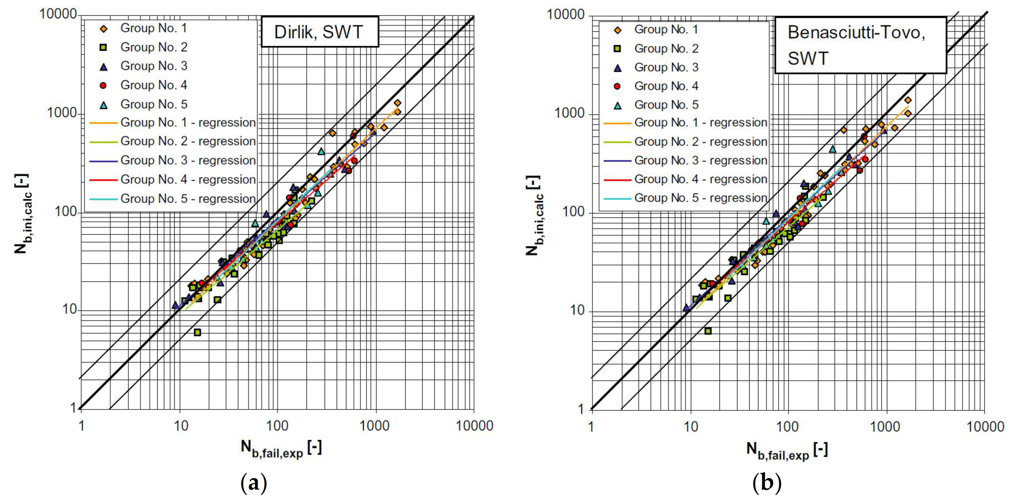
An interesting comprehensive experimental study is presented in [80], where estimations of several spectral methods were compared with experiments from bending and/or torsion random loadings with wide band power spectra of various shape. The multiaxial spectral criterion of [79] was first used to transform the local multiaxial stress into an equivalent uniaxial stress to which spectral methods (Dirlik, TB method, and others) are next applied to estimate the fatigue life by means of Smith‒Watson‒Topper (SWT) parameter [80]. The main conclusion of the experimental study is that the Dirlik and TB methods “proved to be substantially better than the Rayleigh method, and resulted in very small deviations when compared with the experimental data”, as demonstrated by Figure 9.
Interestingly, the study also pointed out how the two spectral methods “give a very similar fatigue life” [80], despite showing essential differences in their rainflow probability distributions. This apparent inconsistency is explained by the fact that both methods have in common that part of the rainflow probability distribution that contributes most to the fatigue damage—this aspect has already been discussed in Section 6.1.
A comparison with experimental data is provided in [61,62] for electronic devices subjected to random loadings, with particular attention on the structural integrity of solder joints in two architectures called package-on-package (PoP) and ball grid array (BGA). The comparison is displayed in Figure 10a. Although the number of test results is not so high to permit general conclusions to be drawn on a statistical basis, some trends emerge clearly. For example, in both the vibration tests the TB method yields estimations within 10% from experiments—note that the Dirlik method was not included in the study [61]. Similar trends were confirmed when other spectral methods were included in the comparison [62]. Again, the few experimental tests point out that, among all spectral methods, “both the Dirlik and Tovo–Benasciutti methods exhibit less than 10% absolute error, which are more accurate than others” [62]. For sure, these two methods are seen to perform much better than the Steinberg three-band method [73] that traditionally is preferred in the field of electronics applications.
As already mentioned in Section 3, the temperature-modified Dirlik method is checked against experimental data obtained in [30,31] by testing a die-casting aluminum alloy at various temperatures. Apart from some scatter in experimental data, the comparison shows that fatigue life can be estimated successfully by the Dirlik method [30,31] (see Figure 10b).
A nice correlation with experimental data, which confirms the capability of spectral methods in predicting fatigue life, is also highlighted in [81] for the Dirlik method—presumably the TB method, though not shown, is close to experimental data as well.
It finally has to be mentioned how the good accuracy of the Dirlik method encompasses not only metallic materials, but also advanced materials as composites [66].
7. Conclusions
Spectral methods are finding more and more application in various engineering areas and with various material types: from testing handheld devices to rocket launchers, from testing common metallic materials to ceramic matrix composites and even to concrete asphalt mortars.
Whether or not a spectral method is accurate enough in a certain application depends, first, on if its hypotheses are satisfied by that application. Methods restricted to narrow band processes will overestimate the damage if applied to a wide band process. Similarly, methods developed for stationary Gaussian processes will be wrong if applied to non-Gaussian or nonstationary processes. For any given application, the decision on which method is more appropriate is left to each one’s engineering judgement.
On the other hand, a certain degree of approximation must be accepted when using spectral methods, since the actual measured random time histories of stress (for example, obtained by measurements) can hardly be exactly stationary and Gaussian, as instead prescribed by the models. The degree of approximation depends on how much the model hypotheses are violated. Sometimes, dividing a nonstationary signal into stationary, or almost-stationary, segments may be a simple and feasible solution. In other cases, especially with irregular time histories, the solution is not so obvious, or may even not exist.
Once it has been verified that a given application matches the model hypotheses, the choice of “the best” model sometimes becomes less obvious, especially for “newcomers” to vibration fatigue. The multitude of spectral methods in the literature may let one feel somehow disoriented, indeed. Help may come from results of comparative studies. As this article pointed out, for wide band stationary Gaussian processes, the literature seems to have found by now a consensus in identifying the methods by Dirlik and by Tovo–Benasciutti (TB) as “the best” spectral methods, with very little—if not even negligible—differences between them. Which one to use then becomes a matter of personal preference.
For what concerns possible areas of development of spectral methods, besides additional studies to evaluate the potential of spectral methods in different industrial sectors using different materials, some research topics could deserve attention in the future: multiaxial fatigue with nonstationary random loadings, crack propagation models, and, finally, the uncertainty in damage estimates due to sampling variability of power spectrum.
For multiaxial fatigue, it is known that the great majority of spectral criteria developed thus far—mostly as reformulations of multiaxial criteria originally in time domain [82,83]—are limited to stationary loadings. A great deal of research is required to extend those criteria to nonstationary multiaxial random loadings, by also considering that the nonstationary case has not yet been solved completely even for uniaxial loadings. At the same time, the development of new multiaxial spectral criteria, either in stationary or nonstationary case, should go hand in hand with experimental testing, aimed at gathering a database for calibrating and validating new multiaxial spectral methods—for example, by testing additively manufactured materials that have recently attracted so much attention by research.
For fatigue crack growth, it seems that the current literature on spectral-based crack propagation models is not so vast [6,7,8,9,10], so this topic may represent quite a promising research field; a starting point may be, for example, the development of spectral methods to include the effect of overloads.
Finally, a topic that, so far, has received very little or almost no attention is the effect on spectral fatigue damage of the sampling variability of a power spectral density computed from short time history records. When this sampling variability is included in the analysis, the fatigue damage estimated by spectral methods becomes a random value with a statistical variability evaluated through confidence intervals. Although some achievements have been obtained recently [84], this topic certainly deserves more attention by research in the years to come.
Author Contributions
Writing—original draft preparation, D.B.; writing—review and editing, T.D. and D.B. All authors have read and agreed to the published version of the manuscript.
Funding
This research received no external funding.
Conflicts of Interest
The authors declare no conflict of interest.
References
- Matsuishi, M.; Endo, T. Fatigue of metals subjected to varying stress. Presented to Japan Society of Mechanical Engineers, Fukuoka, Japan, March 1968. In The Rainflow Method in Fatigue: The Tatsuo Endo Memorial Volume; Murakami, Y., Ed.; Butterworth-Heinemann Ltd.: Oxford, UK, 1992. [Google Scholar]
- ASTM E1049–85 (2017) Standard Practices for Cycle Counting in Fatigue Analysis; ASTM International: West Conshohocken, PA, USA, 2017; Available online: www.astm.org (accessed on 23 August 2021).
- Fatemi, A.; Yang, L. Cumulative fatigue damage and life prediction theories: A survey of the state of the art for homogeneous materials. Int. J. Fatigue 1998, 20, 9–34. [Google Scholar] [CrossRef]
- MATLAB (2021), Version 9.10.0.1602886 (R2021a); The MathWorks Inc.: Natick, MA, USA, 2021; Available online: https://it.mathworks.com (accessed on 3 August 2021).
- Brodtkorb, P.A.; Johannesson, P.; Lindgren, G.; Rychlik, I.; Rydén, J.; Sjö, E. WAFO—A Matlab toolbox for analysis of random waves and loads. In Proceedings of the 10th Int. Offshore and Polar Engineering Conference (ISOPE), Seattle, WA, USA, 27 May–2 June 2000; Volume III, pp. 343–350. [Google Scholar]
- Zuccarello, B.; Adragna, N.F. A novel frequency domain method for predicting fatigue crack growth under wide band random loading. Int. J. Fatigue 2007, 29, 1065–1079. [Google Scholar] [CrossRef]
- Mao, W. Development of a spectral method and a statistical wave model for crack propagation prediction in ship structures. J. Ship Res. 2014, 58, 106–116. [Google Scholar] [CrossRef]
- Xue, X.; Chen, N.Z. Fracture mechanics analysis for a mooring system subjected to Gaussian load processes. Eng. Struct. 2018, 162, 188–197. [Google Scholar] [CrossRef]
- Zhang, Y.; Huang, X.; Wang, F. Fatigue crack propagation prediction for marine structures based on a spectral method. Ocean Eng. 2018, 163, 706–717. [Google Scholar] [CrossRef]
- Marques, D.E.T.; Vandepitte, D.; Tita, V. Damage detection and fatigue life estimation under random loads: A new structural health monitoring methodology in the frequency domain. Fatigue Fract. Eng. Mater. Struct. 2021, 44, 1622–1636. [Google Scholar] [CrossRef]
- Miles, J.W. On structural fatigue under random loading. J. Aeron. Sci. 1954, 21, 753–762. [Google Scholar] [CrossRef]
- Bendat, J.S. Probability Functions for Random Responses: Prediction of Peaks, Fatigue Damage, and Catastrophic Failures; Report NASA-CR-33; National Aeronautics and Space Administration (NASA): Washington, DC, USA, 1964. [Google Scholar]
- Benasciutti, D. Fatigue Analysis of Random Loadings: A Frequency Domain Approach; LAP Lambert Academic Publishing: Saarbrücken, Germany, 2012; ISBN 9783659123702. [Google Scholar]
- Slavič, J.; Boltezar, M.; Mrsnik, M.; Cesnik, M.; Javh, J. Vibration Fatigue by Spectral Methods. From Structural Dynamics to Fatigue Damage—Theory and Experiments; Elsevier: Amsterdam, The Netherlands, 2020. [Google Scholar]
- Dirlik, D. Application of Computers in Fatigue Analysis. Ph.D. Thesis, University of Warwick, Warwick, UK, 1985. [Google Scholar]
- Benasciutti, D.; Tovo, R. Spectral methods for lifetime prediction under wide-band stationary random processes. Int. J. Fatigue 2005, 27, 867–877. [Google Scholar] [CrossRef]
- Benasciutti, D.; Tovo, R. Comparison of spectral methods for fatigue analysis in broad-band Gaussian random processes. Probab. Eng. Mech. 2006, 21, 287–299. [Google Scholar] [CrossRef]
- Lutes, L.D.; Sarkani, S. Random Vibrations: Analysis of Structural and Mechanical Systems; Elsevier Butterworth-Heinemann: Oxford, UK, 2004. [Google Scholar]
- Troncossi, M.; Pesaresi, E. Analysis of synthesized non-Gaussian excitations for vibration-based fatigue life testing. J. Phys. Conf. Ser. 2019, 1264, 012039. [Google Scholar] [CrossRef] [Green Version]
- Vanmarcke, E.H. Properties of spectral moments with applications to random vibration. J. Eng. Mech. Div.-ASCE 1972, 98(EM2), 425–446. [Google Scholar] [CrossRef]
- Hobbacher, A.F. Recommendations for Fatigue Design of Welded Joints and Components, 2nd ed.; IIW document IIW-1823-07 (ex XIII-2151r4-07/XV-1254r4-07); Springer International Publishing: Heidelberg, Germany, 2016. [Google Scholar]
- Wirsching, P.H.; Light, M.C. Fatigue under wide band random stresses. J. Struct. Div. ASCE 1980, 106, 1593–1607. [Google Scholar] [CrossRef]
- Google Scholar. Available online: https://scholar.google.com/scholar?hl=it&as_sdt=0%2C5&q=dirlik+fatigue&btnG= (accessed on 1 August 2021).
- Shinozuka, M. Monte Carlo solution of structural dynamics. Comput. Struct. 1972, 2, 855–874. [Google Scholar] [CrossRef]
- Shinozuka, M.; Deodatis, G. Simulation of stochastic processes by spectral representation. Appl. Mech. Rev. 1991, 44, 191–204. [Google Scholar] [CrossRef]
- Ibe, O.C. Fundamentals of Applied Probability and Random Processes, 2nd ed.; Academic Press: Cambridge, MA, USA, 2004. [Google Scholar]
- Sherratt, F.; Bishop, N.W.M.; Dirlik, T. Predicting fatigue life from frequency domain data. Eng. Integr. 2005, 18, 12–16. [Google Scholar]
- Bouyssy, V.; Naboishikov, S.M.; Rackwitz, R. Comparison of analytical counting methods for Gaussian processes. Struct. Saf. 1993, 12, 35–57. [Google Scholar] [CrossRef]
- Zalaznik, A.; Nagode, M. Frequency based fatigue analysis and temperature effect. Mater. Des. 2011, 32, 4794–4802. [Google Scholar] [CrossRef]
- Zalaznik, A.; Nagode, M. Validation of temperature modified Dirlik method. Comput. Mater. Sci. 2013, 96, 173–179. [Google Scholar] [CrossRef]
- Zalaznik, A.; Nagode, M. Experimental, theoretical and numerical fatigue damage estimation using a temperature modified Dirlik method. Eng. Struct. 2015, 96, 56–65. [Google Scholar] [CrossRef]
- Tovo, R. Cycle distribution and fatigue damage under broad-band random loading. Int. J. Fatigue 2002, 24, 1137–1147. [Google Scholar] [CrossRef]
- Mršnik, M.; Slavič, J.; Boltežar, M. Frequency-domain methods for a vibration-fatigue-life estimation—Application to real data. Int. J. Fatigue 2013, 47, 8–17. [Google Scholar] [CrossRef]
- Xu, J.; Zhang, Y.; Han, Q.; Li, J.; Lacidogna, G. Research on the scope of spectral width parameter of frequency domain methods in random fatigue. Appl. Sci. 2020, 10, 4715. [Google Scholar] [CrossRef]
- Benasciutti, D.; Tovo, R. Modelli di previsione del danneggiamento a fatica per veicoli in regime stazionario ed ergodico. In Proceedings of the Italian Association for Stress Analysis (AIAS), Parma, Italy, 18–20 September 2002. (In Italian). [Google Scholar]
- Benasciutti, D.; Tovo, R. Spectral methods for lifetime prediction under wide-band stationary random processes. In Proceedings of the Int. Conference “Cumulative Fatigue Damage”, Seville, Spain, 27–29 May 2003; p. 46. [Google Scholar]
- Gao, Z.; Moan, T. Frequency-domain fatigue analysis of wide-band stationary Gaussian processes using a trimodal spectral formulation. Int. J. Fatigue 2008, 30, 1944–1955. [Google Scholar] [CrossRef]
- Zhao, W.; Baker, M.J. On the probability density function of rainflow stress range for stationary Gaussian processes. Int. J. Fatigue 1992, 14, 121–135. [Google Scholar] [CrossRef]
- Lutes, L.D.; Larsen, C.E. Improved spectral method for variable amplitude fatigue prediction. J. Struct. Eng.-ASCE 1990, 116, 1149–1164. [Google Scholar] [CrossRef]
- Larsen, C.E.; Lutes, L.D. Predicting the fatigue life of offshore structures by the single-moment method. Probab. Eng. Mech. 1991, 6, 96–108. [Google Scholar] [CrossRef]
- Yaich, A.; El Hami, A. Numerical and experimental investigation on multiaxial fatigue damage estimation of Qualmark chamber test table structures under random vibrations. Mech. Based Des. Struct. Mech. 2021. published online. [Google Scholar] [CrossRef]
- Niesłony, A.; Macha, E. Spectral Method in Multiaxial Random Fatigue; Springer: Berlin, Germany, 2007. [Google Scholar]
- Bel Knani, K.; Benasciutti, D.; Signorini, A.; Tovo, R. Fatigue damage assessment of a car body-in-white using a frequency-domain approach. Int. J. Mater. Prod. Technol. 2007, 30, 172–198. [Google Scholar] [CrossRef]
- Valsamos, G.; Theodosiou, C.; Natsiavas, S. Periodic steady state response and fatigue analysis of a nonlinear city bus model. In Proceedings of the ASME 2009 International Design Engineering Technical Conferences and Computers and Information in Engineering Conference, San Diego, CA, USA, 30 August–2 September 2009. [Google Scholar] [CrossRef]
- Braccesi, C.; Cianetti, F.; Lori, G.; Pioli, D. Random multiaxial fatigue: A comparative analysis among selected frequency and time domain fatigue evaluation methods. Int. J. Fatigue 2015, 74, 107–118. [Google Scholar] [CrossRef]
- Braccesi, C.; Cianetti, F.; Tomassini, L. An innovative modal approach for frequency domain stress recovery and fatigue damage evaluation. Int. J. Fatigue 2016, 91, 382–396. [Google Scholar] [CrossRef]
- Nascimento, V.; Teixeira, G.; Clarke, T. Structural validation of a pneumatic brake actuator using method for fatigue life calculation. Eng. Fail. Anal. 2020, 118, 104837. [Google Scholar] [CrossRef]
- Kong, Y.S.; Abdullah, S.; Schramm, D.; Omar, M.Z.; Haris, S.M. Vibration fatigue analysis of carbon steel coil spring under various road excitations. Metals 2018, 8, 617. [Google Scholar] [CrossRef] [Green Version]
- Wang, N.; Liu, J.; Zhang, Q.; Yang, H.; Tang, M. Fatigue life evaluation and failure analysis of light beam direction adjusting mechanism of an automobile headlight exposed to random loading. Proc. Inst. Mech. Eng. Part D-J. Automob. Eng. 2019, 233, 224–231. [Google Scholar] [CrossRef]
- Cima, M.; Solazzi, L. Experimental and analytical study of random fatigue, in time and frequencies domain, on an industrial wheel. Eng. Fail. Anal. 2021, 120, 105029. [Google Scholar] [CrossRef]
- Ugras, R.C.; Alkan, O.K.; Serkan Orhan, S.; Kutlu, M.; Mugan, A. Real time high cycle fatigue estimation algorithm and load history monitoring for vehicles by the use of frequency domain methods. Mech. Syst. Signal Proc. 2019, 118, 290–304. [Google Scholar] [CrossRef]
- DNV GL. Class Guideline DNVGL-CG-0129, Fatigue Assessment of Ship Structures; DNV GL: Oslo, Norway, 2015; Available online: www.dnv.com (accessed on 23 August 2021).
- Bittar Filho, J.H.; Lourenço de Souza, M.I.; Pasqualino, I.P. Comparison of spectral fatigues methodologies using equivalent stresses obtained by Mises and Battelle applied to a semi-submersible platform. In Practical Design of Ships and Other Floating Structures; Okada, T., Suzuki, K., Kawamura, Y., Eds.; Springer: Singapore, 2019; Volume 64, pp. 580–607. [Google Scholar] [CrossRef]
- Lynch, J.P.; Law, K.H.; O’Connor, S. Probabilistic & Reliability-Based Health Monitoring Strategies for High-Speed Naval Vessels; Report N00014-09-1-0567; Office of Naval Research (ONR): Arlington, VA, USA, 2012. [Google Scholar]
- Yeter, B.; Garbatov, Y.; Guedes Soares, C. Evaluation of fatigue damage model predictions for fixed offshore wind turbine support structures. Int. J. Fatigue 2016, 87, 71–80. [Google Scholar] [CrossRef]
- Böhm, M.; Kowalski, M. Fatigue life estimation of explosive cladded transition joints with the use of the spectral method for the case of a random sea state. Mar. Struct. 2020, 71, 102739. [Google Scholar] [CrossRef]
- Ragan, P.; Lance, M. Comparing estimates of wind turbine fatigue loads using time-domain and spectral methods. Wind Eng. 2007, 31, 83–99. [Google Scholar] [CrossRef]
- Chen, X. Analysis of crosswind fatigue of wind-excited structures with nonlinear aerodynamic damping. Eng. Struct. 2014, 74, 145–156. [Google Scholar] [CrossRef]
- Huo, T.; Tong, L. An approach to wind-induced fatigue analysis of wind turbine tubular towers. J. Constr. Steel. Res. 2020, 166, 105917. [Google Scholar] [CrossRef]
- Fekih, L.B.; Kouroussis, G.; Verlinden, O. Spectral-based fatigue assessment of ball grid arrays under aerospace vibratory environment. Key Eng. Mater. 2013, 569–570, 425–432. [Google Scholar] [CrossRef]
- Xia, J.; Li, G.; Li, B.; Cheng, L.; Zhou, B. Fatigue life prediction of Package-on-Package stacking assembly under random vibration loading. Microelectron. Reliab. 2017, 71, 111–118. [Google Scholar] [CrossRef]
- Xia, J.; Yang, L.; Liu, Q.; Peng, Q.; Cheng, L.; Li, G. Comparison of fatigue life prediction methods for solder joints under random vibration loading. Microelectron. Reliab. 2019, 95, 58–64. [Google Scholar] [CrossRef]
- Gao, D.Y.; Yao, W.X.; Wen, W.D.; Huang, J. Equivalent spectral method to estimate the fatigue life of composite laminates under random vibration loadings. Mech. Compos. Mater. 2021, 57, 101–114. [Google Scholar] [CrossRef]
- Chen, X.; Sun, Y.; Wu, Z.; Yao, L.; Zhang, Y.; Zhou, S.; Liu, Y. An investigation on residual strength and failure probability prediction for plain weave composite under random fatigue loading. Int. J. Fatigue 2019, 120, 267–282. [Google Scholar] [CrossRef]
- Sun, Y.; Zhang, Y.; Yang, C.; Liu, Y.; Chen, X.; Yao, L.; Gao, W. Prediction on fatigue properties of the plain weave composite under broadband random loading. Fatigue Fract. Eng. Mater. Struct. 2021, 44, 1515–1532. [Google Scholar] [CrossRef]
- Böhm, M.; Głowacka, K. Fatigue life estimation with mean stress effect compensation for lightweight structures—The case of GLARE 2 composite. Polymers 2020, 12, 251. [Google Scholar] [CrossRef] [Green Version]
- Kim, H.; Kim, G.; Ji, W.; Lee, Y.S.; Jang, S.; Shin, C.M. Random vibration fatigue analysis of a multi-material battery pack structure for an electric vehicle. Funct. Compos. Struct. 2021, 3, 025006. [Google Scholar] [CrossRef]
- Zhou, Y.; Wu, S.; Tan, Z.; Fei, Q. Temperature-dependence of acoustic fatigue life for thermal protection structures. Theor. Appl. Mech. Letters 2014, 4, 021005. [Google Scholar] [CrossRef] [Green Version]
- Česnik, M.; Slavič, J.; Boltežar, M. Assessment of the fatigue parameters from random vibration testing: Application to a rivet joint. Strojniski Vestn.-J. Mech. Eng. 2016, 62, 471–482. [Google Scholar] [CrossRef]
- Go, E.-S.; Kim, M.-G.; Kim, I.-G.; Kim, M.-S. Fatigue life prediction in frequency domain using thermal-acoustic loading test results of titanium specimen. J. Mech. Sci. Technol. 2020, 34, 4015–4024. [Google Scholar] [CrossRef]
- Ding, H.; Zhu, Q.; Zhang, P. Fatigue damage assessment for concrete structures using a frequency-domain method. Math. Probl. Eng. 2014, 2014, 407193. [Google Scholar] [CrossRef]
- Ortiz, K.; Chen, N.K. Fatigue damage prediction for stationary wide-band stresses. In Reliability and Risk Analysis in Civil Engineering, Proceedings of the 5th International Conference on the Applications of Statistics and Probability in Soil and Structural Engineering (ICASP5), Vancouver, Canada, 25–29 May 1987; Institute for Risk Research, University of Waterloo: Waterloo, ON, Canada, 1987. [Google Scholar]
- Steinberg, D.S. Vibration Analysis for Electronic Equipment, 3rd ed.; Wiley-Interscience: New York, NY, USA, 2000. [Google Scholar]
- Fu, T.-T.; Cebon, D. Predicting fatigue lives for bi-modal stress spectral densities. Int. J. Fatigue 2000, 22, 11–21. [Google Scholar] [CrossRef]
- Benasciutti, D.; Tovo, R. On fatigue damage assessment in bimodal random processes. Int. J. Fatigue 2007, 29, 232–244. [Google Scholar] [CrossRef]
- Lalanne, C. Mechanical Vibration and Shock; Hermes Penton Science: London, UK, 2009. [Google Scholar]
- Larsen, C.E.; Irvine, T. A review of spectral methods for variable amplitude fatigue prediction and new results. Procedia Eng. 2015, 101, 243–250. [Google Scholar] [CrossRef] [Green Version]
- Han, Q.; Li, J.; Xu, J.; Ye, F.; Carpinteri, A.; Lacidogna, G. A new frequency domain method for random fatigue life estimation in a wide-band stationary Gaussian random process. Fatigue Fract. Eng. Mater. Struct. 2019, 42, 97–113. [Google Scholar] [CrossRef] [Green Version]
- Niesłony, A. Comparison of some selected multiaxial fatigue failure criteria dedicated for spectral method. J. Theor. Appl. Mech. 2010, 48, 233–254. [Google Scholar]
- Niesłony, A.; Růžička, M.; Papuga, J.; Hodr, A.; Balda, M.; Svoboda, J. Fatigue life prediction for broad-band multiaxial loading with various PSD curve shapes. Int. J. Fatigue 2012, 44, 74–88. [Google Scholar] [CrossRef] [Green Version]
- Gadolina, I.V.; Makhutov, N.A.; Erpalov, A.V. Varied approaches to loading assessment in fatigue studies. Int. J. Fatigue 2021, 144, 106035. [Google Scholar] [CrossRef]
- Benasciutti, D.; Sherratt, F.; Cristofori, A. Recent developments in frequency domain multi-axial fatigue analysis. Int. J. Fatigue 2016, 91, 397–413. [Google Scholar] [CrossRef]
- Carpinteri, A.; Spagnoli, A.; Vantadori, S. A review of multiaxial fatigue criteria for random variable amplitude loads. Fatigue Fract. Eng. Mater. Struct. 2017, 40, 1007–1036. [Google Scholar] [CrossRef]
- Benasciutti, D. Confidence interval of the ‘single-moment’ fatigue damage calculated from an estimated power spectral density. Int. J. Fatigue 2021, 145, 106131. [Google Scholar] [CrossRef]
Figure 1.
(a) Time history samples and (b) their PSD (narrow band, wide band, bimodal).

Figure 2.
Types of PSD used in numerical simulations used to develop the Dirlik method: (a) rectangular bimodal spectrum; (b) smooth spectrum. Figures are from [15].
Figure 2.
Types of PSD used in numerical simulations used to develop the Dirlik method: (a) rectangular bimodal spectrum; (b) smooth spectrum. Figures are from [15].

Figure 3.
Probability distribution of: (a) simple ranges; (b) rainflow ranges. The numbers correspond to the irregularity factor of smooth PSD. On the x-axis, values are normalized as [15].
Figure 3.
Probability distribution of: (a) simple ranges; (b) rainflow ranges. The numbers correspond to the irregularity factor of smooth PSD. On the x-axis, values are normalized as [15].

Figure 4.
Amplitude–mean probability distributions in TB method: (a) level crossing counting; (b) approximate range counting. Representation of is only qualitative, as it includes a Dirac delta function for and . Reproduced from [32] with permission from Elsevier.
Figure 4.
Amplitude–mean probability distributions in TB method: (a) level crossing counting; (b) approximate range counting. Representation of is only qualitative, as it includes a Dirac delta function for and . Reproduced from [32] with permission from Elsevier.

Figure 5.
Power spectral densities used in simulations to calibrate weight in TB method.

Figure 6.
Comparison of (a) rainflow probability distributions, (b) weighted by the damage per amplitude. The figures refer to parameters , (with , ).
Figure 6.
Comparison of (a) rainflow probability distributions, (b) weighted by the damage per amplitude. The figures refer to parameters , (with , ).

Figure 7.
Comparison of (a) rainflow probability distributions, (b) weighted by the damage per amplitude. The figures refer to parameters , (with , ).
Figure 7.
Comparison of (a) rainflow probability distributions, (b) weighted by the damage per amplitude. The figures refer to parameters , (with , ).

Figure 8.
Example of comparison in [37] with the same power spectra used (a) in [16] and (b) in [15] (SS = simple sum of damage of frequency components in trimodal spectrum, NB = narrow band formula in Equation (5), DK = Dirlik, BT = TB method, Proposed = method proposed in [37]). Reproduced from [37] with permission from Elsevier.

Figure 9.
Example of comparison with experimental fatigue life presented in [80] for: (a) Dirlik method and (b) TB method. Reproduced from [80] with permission from Elsevier.

Figure 10.
Comparison with experimental data: (a) electronic application for package-on-package (PoP) and ball grid array (BGA) (DK = Dirlik, TB = TB method, ZB = Zhao‒Baker, SM = single-moment, ST = Steinberg method, WL = Wirsching‒Light) (b) temperature effect on random loading (DTMDK = temperature modified Dirlik method). Reproduced from [30,62] with permission from Elsevier.


Table 1.
Parameters of some types of narrow band, band-limited, and bimodal power spectral densities for which Dirlik and TB methods are compared ( in Hz, μ peaks per second, crossing per second, n.a. = not applicable).
Table 1.
Parameters of some types of narrow band, band-limited, and bimodal power spectral densities for which Dirlik and TB methods are compared ( in Hz, μ peaks per second, crossing per second, n.a. = not applicable).
| PSD | c | ||||||||||
|---|---|---|---|---|---|---|---|---|---|---|---|
| b = 3 | b = 5 | b = 7 | |||||||||
| Narrow band | 1.05 | n.a. | 0 | 19.50 | 0.9999 | 0.9996 | 20 | 19.99 | 0.9999 | 0.9997 | 0.9996 |
| 1.10 | n.a. | 0 | 19.01 | 0.9996 | 0.9985 | 20 | 19.97 | 0.999 | 0.999 | 0.998 | |
| Band limited | 1.50 | n.a. | 0 | 15.50 | 0.993 | 0.975 | 20 | 19.50 | 0.991 | 0.981 | 0.969 |
| 5 | n.a. | 0 | 5.14 | 0.933 | 0.827 | 20 | 16.54 | 0.980 | 0.920 | 0.867 | |
| 20 | n.a. | 0 | 1.29 | 0.886 | 0.765 | 20 | 15.29 | 0.998 | 0.932 | 0.875 | |
| ∞ | n.a. | 0 | 0.0 | 0.866 | 0.745 | 20 | 14.91 | 1.00 | 0.943 | 0.885 | |
| Bimodal | 1.1/0.9 | 2.981 | 0.098 | 8.258 | 0.900 | 0.600 | 20 | 12.00 | 0.983 | 0.963 | 0.954 |
| 1.1/0.9 | 7.408 | 0.006 | 4.677 | 0.900 | 0.300 | 20 | 6.00 | 0.929 | 0.966 | 0.964 | |
| 1.1/0.9 | 3.233 | 0.240 | 6.409 | 0.850 | 0.600 | 20 | 12.00 | 0.996 | 0.944 | 0.922 | |
| 1.1/0.9 | 7.176 | 0.050 | 2.920 | 0.700 | 0.300 | 20 | 6.00 | 1.000 | 0.989 | 0.992 | |
| 1.1/0.9 | 11.855 | 0.025 | 1.705 | 0.600 | 0.200 | 20 | 4.00 | 1.035 | 1.025 | 1.026 | |
| 1.1/0.9 | 11.715 | 0.051 | 1.628 | 0.550 | 0.250 | 20 | 5.00 | 1.060 | 1.029 | 1.027 | |
| 1.1/0.9 | 19.442 | 0.014 | 1.001 | 0.503 | 0.139 | 20 | 2.78 | 1.062 | 1.052 | 1.052 | |
Publisher’s Note: MDPI stays neutral with regard to jurisdictional claims in published maps and institutional affiliations. |
© 2021 by the authors. Licensee MDPI, Basel, Switzerland. This article is an open access article distributed under the terms and conditions of the Creative Commons Attribution (CC BY) license (https://creativecommons.org/licenses/by/4.0/).
Share and Cite
MDPI and ACS Style
Dirlik, T.; Benasciutti, D. Dirlik and Tovo-Benasciutti Spectral Methods in Vibration Fatigue: A Review with a Historical Perspective. Metals 2021, 11, 1333. https://doi.org/10.3390/met11091333
AMA Style
Dirlik T, Benasciutti D. Dirlik and Tovo-Benasciutti Spectral Methods in Vibration Fatigue: A Review with a Historical Perspective. Metals. 2021; 11(9):1333. https://doi.org/10.3390/met11091333
Chicago/Turabian StyleDirlik, Turan, and Denis Benasciutti. 2021. "Dirlik and Tovo-Benasciutti Spectral Methods in Vibration Fatigue: A Review with a Historical Perspective" Metals 11, no. 9: 1333. https://doi.org/10.3390/met11091333
Note that from the first issue of 2016, this journal uses article numbers instead of page numbers. See further details here.