Optical Machine Learning Using Time-Lens Deep Neural NetWorks
by
 ,
,
Luhe Zhang
1, 
Caiyun Li
1,
Jiangyong He
1,
Yange Liu
1,
Jian Zhao
2,
Huiyi Guo
1,
Longfei Zhu
1,
Mengjie Zhou
1,
Kaiyan Zhu
1,
Congcong Liu
1 and
Zhi Wang
1,* 1
Tianjin Key Laboratory of Optoelectronic Sensor and Sensing Network Technology, Institute of Modern Optics, Nankai University, Tianjin 300350, China
2
Key Laboratory of Opto-Electronic Information Technical Science of Ministry of Education, School of Precision Instruments and Optoelectronics Engineering, Tianjin University, Tianjin 300372, China
*
Author to whom correspondence should be addressed.
Photonics 2021, 8(3), 78; https://doi.org/10.3390/photonics8030078
Submission received: 25 February 2021
/
Revised: 12 March 2021
/
Accepted: 12 March 2021
/
Published: 15 March 2021
(This article belongs to the Special Issue Advanced Technique and Future Perspective for Next Generation Optical Fiber Communications)
Abstract
:As a high-throughput data analysis technique, photon time stretching (PTS) is widely used in the monitoring of rare events such as cancer cells, rough waves, and the study of electronic and optical transient dynamics. The PTS technology relies on high-speed data collection, and the large amount of data generated poses a challenge to data storage and real-time processing. Therefore, how to use compatible optical methods to filter and process data in advance is particularly important. The time-lens proposed, based on the duality of time and space as an important data processing method derived from PTS, achieves imaging of time signals by controlling the phase information of the timing signals. In this paper, an optical neural network based on the time-lens (TL-ONN) is proposed, which applies the time-lens to the layer algorithm of the neural network to realize the forward transmission of one-dimensional data. The recognition function of this optical neural network for speech information is verified by simulation, and the test recognition accuracy reaches 95.35%. This architecture can be applied to feature extraction and classification, and is expected to be a breakthrough in detecting rare events such as cancer cell identification and screening.
1. Introduction
Recently, artificial neural networks (ANNs) have achieved significant developments rapidly and extensively. As the fastest developing computing method of artificial intelligence, deep learning has made remarkable achievements in machine vision [1], image classification [2], game theory [3], speech recognition [4], natural language processing [5], and other aspects. The use of elementary particles for data transmission and processing can lead to smaller equipment, greater speed, and lower energy consumption. The electron is the most widely used particle to date, and has become the cornerstone of the information society in signal transmission (cable) and data processing (electronic computer). Artificial intelligence chips represented by graphics processing units (GPUs), application-specific integrated circuits (ASICs), and field programmable gate arrays (FPGAs) have enabled electronic neural networks (ENNs) to achieve high precision, high convergence regression, and predict task performance [6]. When dealing with tasks with high complexity and high data volume, insurmountable shortcomings have emerged in ENNs, such as long time delay and low power efficiency caused by the interaction of many parameters in the network with the storage modules of electronic devices.
Fortunately, as a kind of boson, the photon has faster speed and lower energy consumption, resulting in it being significantly better than electrons in signal transmission and processing, and it has become a strong competitor for the elementary particles used in the next generation of information technology. Development of all-optical components, photonic chips, interconnects, and processors will bring the speed of light, photon coherence properties, field confinement and enhancement, information-carrying capacity, and the broad spectrum of light into the high-performance computing, the internet of things, and industries related to cloud, fog, and recently edge computing [7]. Due to the parallel characteristics of light in propagation, light interference, diffraction, and dispersion, phenomena can easily simulate various matrix linear operations, which are similar to the layer algorithm of forward propagation in neural networks. To pursue faster operating speed and higher power efficiency in information processing, the optical neural network (ONN), which uses photons as the information carrier, came at the right moment. Various ONN architectures have been proposed, including the optical interference neural network [8], the diffractive optical neural network [9,10,11,12], photonic reservoir computing [13,14], the photonic spiking neural network [15], and the recurrent neural network [16]. To process high-throughput and high-complexity data in real time, the algorithms in ONNs must have the characteristics of real-time information collection and rapid information measurement.
Photon time stretching (PTS), also known as dispersive Fourier transform technology (DFT), is a high-throughput real-time information collection technology that has emerged in recent years [17]. PTS can overcome the limitations of electronic equipment bandwidth and sampling speed, thus being able to realize ultra-fast information measurement, and its imaging frame rate is mainly determined by the mode-locked laser, which can reach tens of MHz/s or even GHz/s. DFT is widely used in ultra-high-speed microscopic imaging, microwave information analysis, spectral analysis, and observation of transient physical processes such as dissipative soliton structure, relativistic electron clusters, and rough waves [18]. It is worth emphasizing that this architecture plays an important role in the capture of rare events such as the early screening of cancer cells with large data volume characteristics. DFT broadens the pulse-carrying cell characteristics in the time domain and maps spectral information to the time domain; then, the information of the stretched light pulse is obtained through photo detection and a high-speed analog-to-digital converter, and finally the information is input into a computer or a special data signal processing chip for data processing. In 2009, researchers in the United States first proposed a method to achieve ultrafast imaging using PTS technology [19]. They then combined ultra-fast imaging and deep learning technology to distinguish colon cancer cells in the blood in 2016 [20]. In 2017, researchers from the University of Hong Kong reduced the monitoring of phytoplankton communities and used support vector machines to classify them, which can detect 100,000–1,000,000 cells per second [21]. In biomedicine, the combination of DFT and optical fluidics technology can complete high-flux imaging of hundreds of thousands to millions of cells per second, including various conditions in human blood and algae cells. It has great significance in cell classification [20], early cell screening [22,23,24] and feature extraction [25,26,27,28,29].
The high-throughput characteristics of PTS technology will inevitably produce a lot of data. Typically, the amount of data generated by a PTS system can reach 1 Tbit per second, which brings huge challenges to data storage and processing based on electronic devices and limits the application scope of this technology [30]. The high-throughput data generation of the DFT and the high-throughput processing characteristics of the photon neural network are perfectly complementary. Based on this characteristic, we propose a new architecture combining time-lens with the optical neural network (TL-ONN). According to the optical space–time duality [31] (that is, the spatial evolution characteristics of the light field caused by the diffraction effect and the time evolution characteristics of the optical pulse caused by the dispersion effect are equivalent), the imaging of the time signal can be realized by controlling the phase information of the timing signal, namely the time-lens. We establish a numerical model for simulation analysis to verify the feasibility of this architecture. By training 20,000 sets of speech data, we obtained a stable 98% recognition accuracy within one training cycle, which has obvious advantages of faster convergence and stable recognition accuracy compared with a deep neural network (DNN) with the same number of layers. This architecture implemented with all-optical components will offer outstanding improvements in biomedical science, cell dynamics, nonlinear optics, green energy, and other fields.
Here, we first introduce the architectural composition of the proposed TL-ONN, and then combine the time-lens principle with the neural network to drive the forward propagation and reverse optimization process. Finally, we use a speech dataset to train the proposed TL-ONN, and use numerical calculation to verify the classification function of this architecture.
2. Materials and Methods
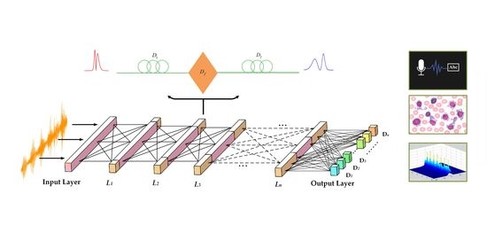
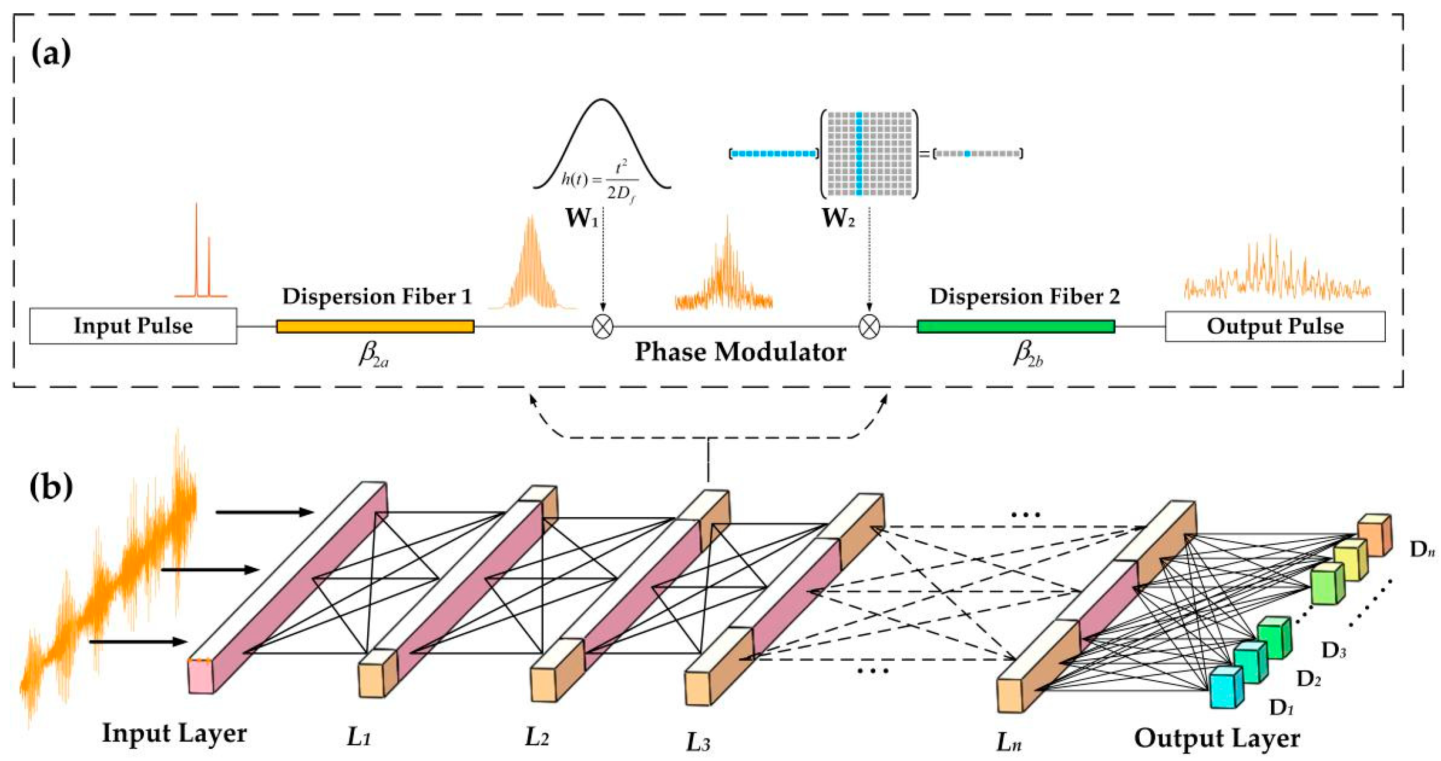
The proposed ONN combines the conventional neural network with time stretch, realizing the deep learning function based on optics. As shown in Figure 1, two kinds of operations—time-lens transform and matrix multiplication—must be performed in each layer. The core optical structure which adapts the time-lens method is used to implement the first linear computation process. After that, the results are modulated by a weights matrix. Finally, the outputs serve as the input vector in the next layer. After calculation by the neural network composed of multiple time-lens layers, all input data are probed by a detector in the output layer. The prediction data and the target output are calculated by the cost function, and the gradient descent algorithm is carried out for each weights matrix (W2) from backward propagation to achieve the optimal neural network structure. The input data of this network structure are generally one-dimensional time data. In the input layer, the physical information at each point in the time series is transferred to the neurons in each layer. Through the optical algorithm, each neuron between the layers is transmitted to realize the information processing behavior of the neural network.
Like the diffraction of space light, the time-lens plays a role of dispersion in time. As a result, the time-lens [32] can realize the imaging of the light pulse on the time scale. This is similar to the idea that the neurons in each layer of the neural network are derived from each neuron in the previous layer through a specific algorithm. The amplitude and phase of each point of the pulse after the time-lens is derived from the previous pulse calculated for each point. Based on this algorithm, an optical neural network based on the time lens is designed. Each neural network layer is formed by two segments of dispersive fiber and a second-order phase factor. The two layers are transmitted through intensity or a phase modulator. After backward propagation, each modulation factor is optimized by the gradient descent algorithm to obtain the best architecture.
2.1. Time-Lens Principle and Simulation Results
Analogous to the process by which a thin lens can image an object in space, a time-lens can image sequences in the time domain, such as laser pulses and sound sequences. In this section, we will introduce the principle of a time-lens starting from the propagation of narrow-band light pulses.
Assuming that the propagation area is infinite, the electric field envelop of a narrow-band laser pulse with a center frequency of propagation in space coordinates and time satisfies
where is the electric field envelope of the input light pulse, is the dispersion coefficient, and represents the angular frequency. Expanding the dispersion coefficient with Taylor series and retaining it to the second order, the frequency spectrum after Fourier transformation can be described as
Then, we perform the inverse Fourier transform on (2) to obtain the time domain pulse envelope:
where is the group velocity, . If we establish a new coordinate whose frame moves at the speed of the group velocity of light, the corresponding transformation can be described as
where and are the time and the space initial points, respectively. Under this circumstance, (3) can be simplified as
Then, we can get the spectrum of the signal envelope by Fourier transform:
where is the time variable in frequency domain, is the imaginary number. It can be seen from the time domain envelope equation that the second order phase modulation of the independent variable T is carried out in the time-lens algorithm. Like the space lens, the space diffraction equation of a paraxial beam and the propagation equation of a narrow-band optical pulse in the dispersive medium both modulate the independent variable (x, y, and t) second order.
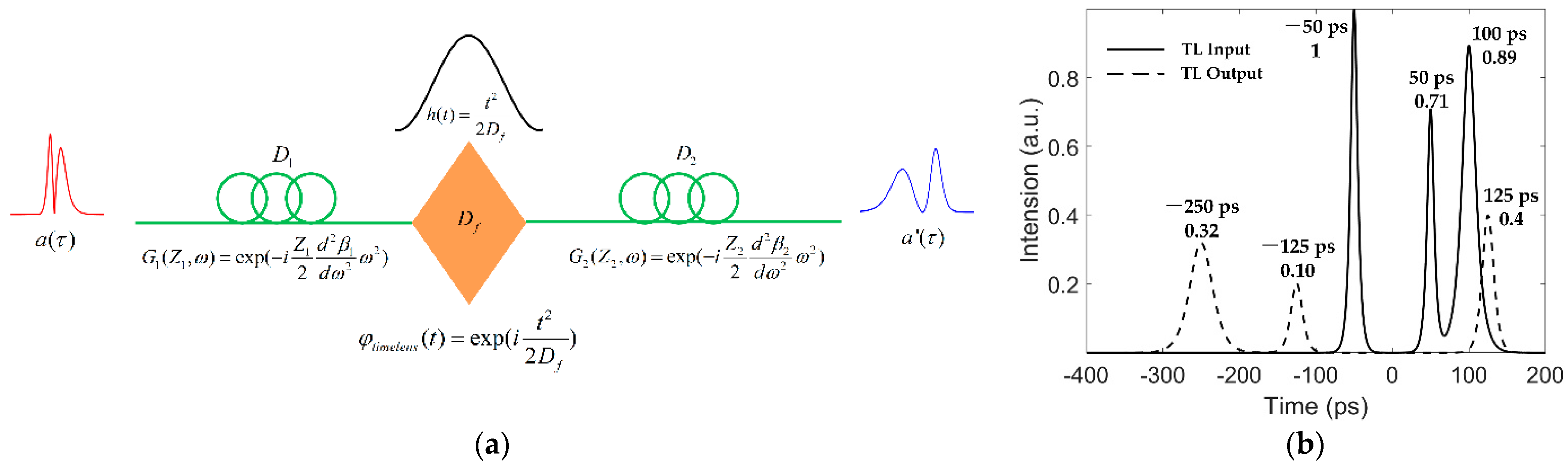
The time lens mainly comprises three parts—the second-order phase modulator and the dispersion medium before and after the modulator (Figure 2a). In the dispersion medium part, the pulse passing through the long distance dispersion fiber is equivalent to the pulse being modulated in the frequency domain by a factor determined by the fiber length and the second-order dispersion coefficient, which can be expressed as
where
and represent the length of fiber i and the second-order dispersion coefficient, respectively. When passing through the time domain phase modulator, the phase factor satisfying the imaging condition of the time-lens is the quadratic function of time by
, and is the focal length of the time-lens satisfying the imaging conditions of the time-lens. With respect to analog space-lens imaging conditions, the time-lens imaging condition is
Its magnification can be expressed as (see Appendix A). Figure 2b shows a comparison of the duration of a group of soliton pulses and their output of the time lens at M = 2.5; the peak position and normalized intensity of the pulse are marked to verify its magnification. In summary, after passing through the time-lens, the pulse is times larger in amplitude and M times larger in duration, and a second order phase modulation is added in phases.
2.2. Mathematical Analysis of TL-ONN
In this section, we will analyze the transmission process of input data in two adjacent time-lens layers. Suppose that the input pulse can be expressed as , that is, the initial intensity in time of the pulse into the first dispersion fiber of the time lens. The intensity of the input data at each time point will be mapped to all time points according to a specific algorithm after two segments of the dispersion fiber in the time lens and second-order phase modulation in the time domain. Equation (9) shows the algorithm results; its derivation can be found in Appendix A. In the neural network based on this algorithm, each neuron in the mth layer can be regarded as the result of mapping all neurons in the (m − 1)th layer.
where represents the magnification factor of the time-lens, and are the second-order dispersion coefficients of the two segments of the dispersion fiber, and are the lengths of the two segments of the dispersion fiber, l represents the layer number, represents all neurons that contribute to the neuron in the lth layer.
The intensity and phase of the neuron in the L layer are determined by both the input pulse in the L − 1 layer and the modulation coefficient in the L layer. For the Lth layer of the network, the information on each neuron can be expressed by
where is the input pulse to neuron of layer , represents the contribution of the k-th neuron of the layer l − 1 to the neuron of the layer l. is the modulation coefficient of the neuron in layer l; the modulation coefficient of a neuron comprises amplitude and phase items, i.e., .
The forward model of our TL-ONN architecture is illustrated in Figure 1 and notated as follows:
where refers to a neuron of the lth layer, and k refers to a neuron of the previous layer, connected to neuron by optical dispersion. The input pulse , which is located at layer 0 (i.e., the input plane), is in general a complex-valued quantity and can carry information in its phase and/or amplitude channels.
Assuming that the TL-ONN design is composed of N layers (excluding the input and output planes), the data transmitted through the architecture are finally detected by PD, and detectors are placed at the output plane to measure the intensity of the output data. If the bandwidth of the PD is much narrower than the output signal bandwidth, the PD will serve not only as an energy transforming device but also as a pulse energy accumulator. The final output of the architecture can be expressed as
where represents the neuron of the output layer (N), and is the energy accumulation coefficient of PD on the time axis of the data.
To train a TL-ONN design, we used the error back-propagation algorithm along with the stochastic gradient descent optimization method. A loss function was defined to evaluate the performance of the network parameters to minimize the loss function. Without loss of generality, here we focus on our classified architecture and define the loss function (E) using the cross-entropy error between the output plane intensity and the target :
In the network based on a time-lens algorithm consisting of N time-lens layers, the data characteristics in the previous layer with neurons are extracted into neurons in the current layer with neurons, where and
represents the scaling multiples between the (L − 1)th layer and the Lth layer. The time-lens algorithm has a similar function of removing the redundant information and compressing the features as the pooling layer in a conventional ANN. The characteristics carried by the input data will emerge and be highlighted through each layer after being transmitted through this classification architecture, and finally evolve into the labels of the corresponding category.
3. Results
In order to verify the effectiveness of the system in the time-domain information classification, we used numerical methods to simulate the TL-ONN to realize the recognition of specific sound signals. We used a dataset containing 18,000 training data and 2000 test data picked from intelligent speech database [33] to evaluate the performances of TL-ONN. The content in the speech dataset is the wake phrase “Hi, Miya!” in English and Chinese collected in the actual home environment using a microphone array and Hi-Fi microphone. The test subset provides paired target/non-target answers to evaluate verification results. In general, we used the dichotomy problem to test the classification performances of two kinds of systems including the TL-ONN and the conventional DNN.
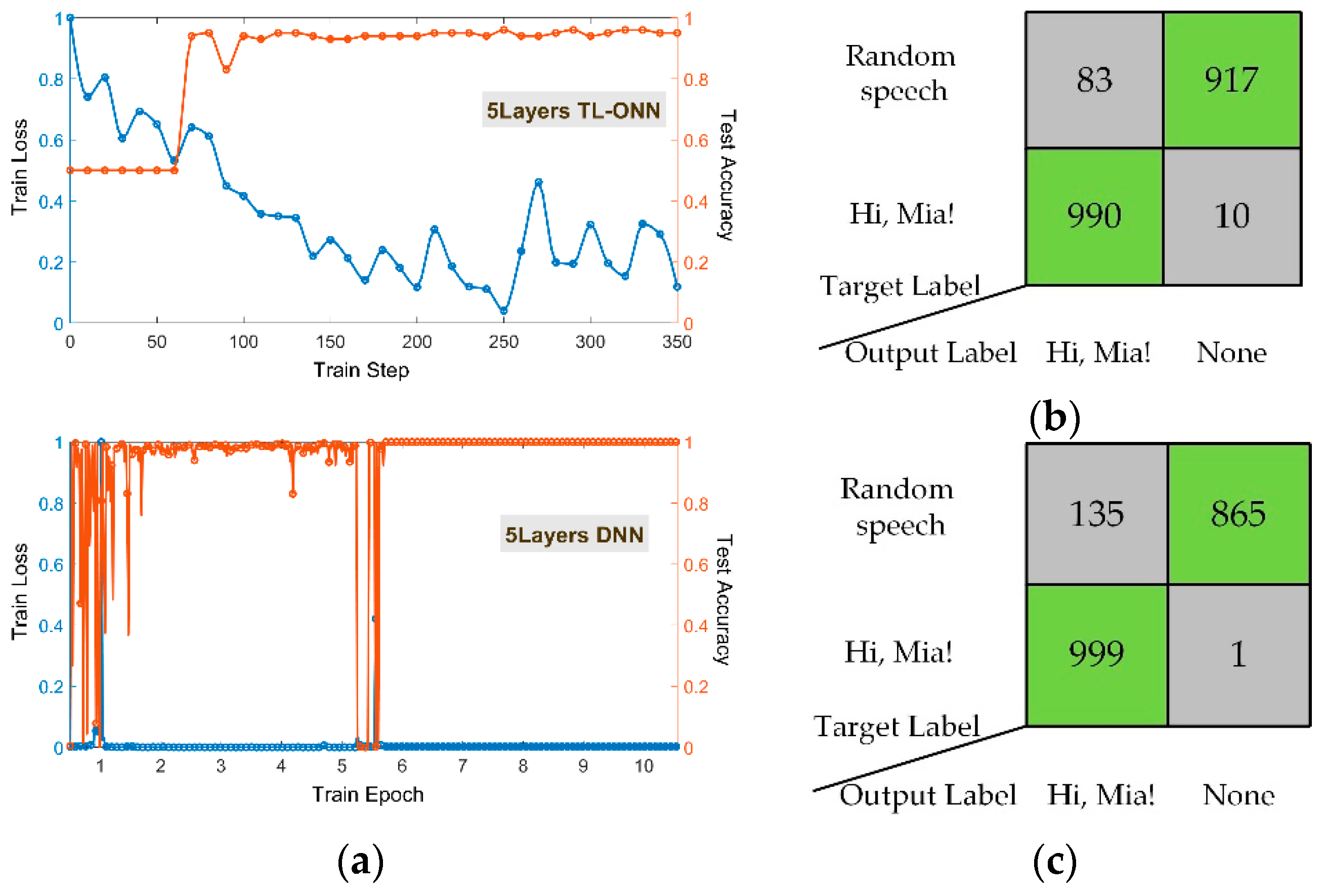
We first constructed a TL-ONN composed of five time-lens layers to verify the classification feasibility of this architecture. Figure 3a shows the training results of TL-ONN in the cases of
. The accuracy of the TL-ONN for a total of 2000 test samples is above 98% (Figure 3a top), which is close to the accuracy for the DNN (Figure 3a bottom). The horizontal axis represents the number of training steps in one training batch (batch size = 50). The accuracy of this test fluctuates greatly in the first few steps, and then reaches over 98% at about 17 steps and remains stable. In contrast, it was difficult for a five-layer DNN network under the same conditions to achieve stable accuracy and training loss in one epoch (Figure 3a). When the training epoch was set to 10, it was found that the test accuracy and training loss still changed suddenly at the 10th training epoch, which might be due to gradient explosion, overfitting, or another reason. We define the accuracy as the proportion of the number of output labels that are the same as the target label to the total number of test sets. Using the same 2000 test set to test the two networks’ architecture, the accuracy rates reached 95.35% (Figure 3b) and 93.2% (Figure 3c). In general, TL-ONN has significant advantages over DNN in verifying classification performance.
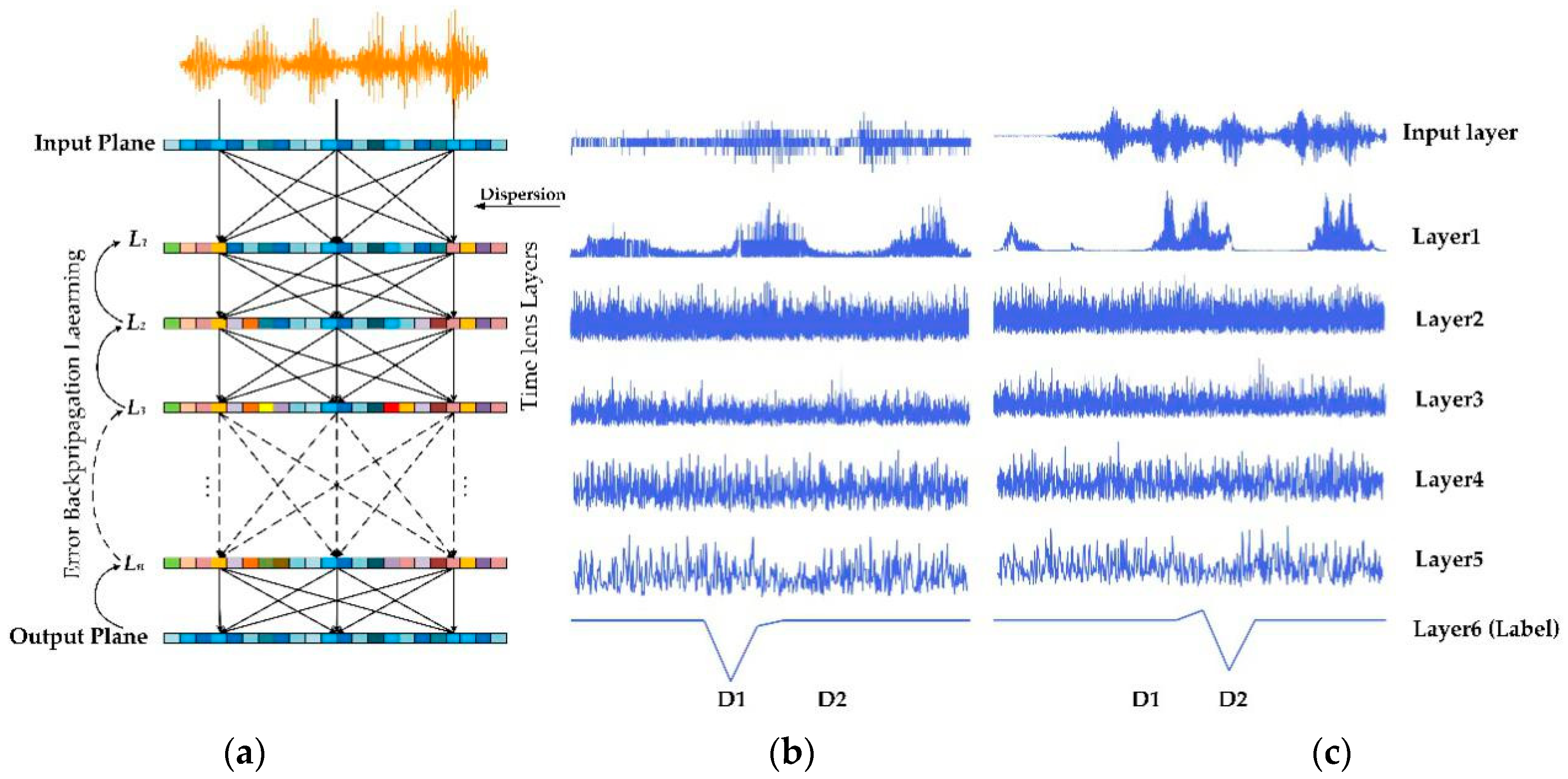
To easily see the changes of the two types of voice information in each layer of TL-ONN, we extracted two sets of input with typical characteristics for observation. Figure 4a shows the layer structure of this network, which contains multiple time-lens layers, where each time point on a given layer acts as a neuron with a complex dispersion coefficient. Figure 4b,c shows the data evolution of each layer when two types of speech are input to the network. From the input layer, we can distinguish the differences between the two types of input data from the shape of the waveform. The waveform containing “Hi, Miya!” has a higher continuity, while the waveform of random speech has quantized characteristics and always has a value on the time axis. On the second layer of the network, the “Hi, Miya!” input will change into several sets of pulses through the time-lens layer and another type of information will spread all over the time. After being transmitted by multiple time-lens layers, the two inputs will eventually change to the shape in Layer 6, and the two types of speech will eventually evolve into the shape of the impact function at different time points. As shown in Figure 4b,c, D1 and D2 correspond to detectors of different input types. The random speech eventually responds at D1, while the input containing “Hi, Miya!” responds at D2.
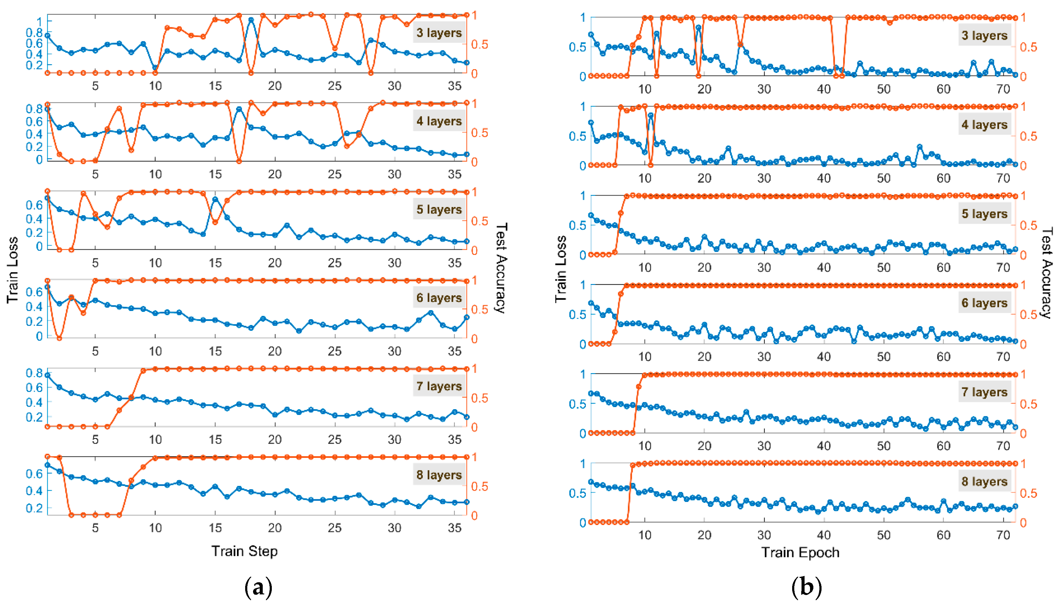
To eliminate the contingency of the experiment, we set up a series of networks consisting of 3–8 layers to test the influence of different numbers of time-lens layers on classification performance. Figure 5 shows the test results of the TL-ONN architecture composed of different numbers of time-lens layers—33, 30, and17 steps are needed in the TL-ONN with three, four, and five layers, respectively, to reach an accuracy of 98% (Figure 5a). When the number of time-lens layers is increased to six or more, the accuracy can be stabilized at 98–99% after about 10 training steps; however, an unlimited increase in the number of time-lens layers does not make the results of network training infinitely better. For example, we can see that compared with a network with six, seven, or eight layers, TL-ONN requires more steps to achieve stable accuracy. Overall, the network with six time-lens layers has the best classification performance. All the results discussed above occur in one training epoch. At least a few epochs were needed to achieve stable classification accuracy for conventional DNN with the same dataset. TL-ONN has obvious advantages of faster convergence speed and stable classification accuracy.
Similarly, we reverse the order of the phase modulator W1 and W2, and use the same training set for training. Figure 5b shows the classification results under this architecture, and the time-scaling multiple between two layers is still 0.6. Under the same conditions, a series of networks consisting of three–eight layers were constructed to test the classification performance. To achieve an accuracy of 98%, 55 and 12 steps are needed in the TL-ONN with three and four layers, respectively. The accuracy can be stabilized at 98–99% after about 10 training steps when the number of time-lens layers is increased to five or more. As with the previous results, compared with a network with six, seven, or eight layers, TL-ONN requires more steps to achieve stable accuracy. Overall, the network structure with six time-lens layers has the best classification performance, and it is consistent with the results of the former architecture.
At the detector/output plane, we measured the intensity of the network output, and as a loss function to train the classification TL-ONN, we used its mean square error (MSE) against the target output. The classification of TL-ONN was trained using a modulator (W2), where we aimed to maximize the normalized signal of each target’s corresponding detector region, while minimizing the total signal outside of all the detector regions. We used the stochastic gradient descent algorithm, Adam [34], to back-propagate the errors and update the layers of the network to minimize the loss function. The classifier TL-ONN was trained with speech datasets [33], and achieved the desired mapping functions between the input and output planes after five steps. The training batch size was set to be 50 for the speech classifier network. To verify the feasibility of the TL-ONN architecture, we used the python language to establish a simulation model for theoretical analysis. The networks were implemented using Python version 3.8.0. and PyTorch version 1.4.0. Using a desktop computer (GeForce GTX 1060 Graphical Processing Unit, GPU and Intel(R) Core (TM) i7-8700 CPU @3.20GHz and 64GB of RAM, running a Windows 10 operating system, Microsoft), the above-outlined PyTorch-based design of a TL-ONN architecture took approximately 26 h to train for the classifier networks.
Compared with conventional DNNs, TL-ONN is not only a physical and optical neural network but also has some unique architecture. First, the time-lens algorithm applied at each layer of the network can refine the features of the input data, similar to what is used as a pooling layer, remove redundant information, and compress features. The time-lens method can be regarded as the pooling element in the photon. Second, TL-ONN can handle complex values, such as complex nonlinear dynamics in passively mode-locked lasers. The phase modulators can respectively modulate different physical parameters, and as long as the modulator parameters are determined, a passive all-optical neural network can be basically realized. Third, the output of each neuron is coupled to the neurons in the next layer through a certain weight relationship through the dispersion effect of the optical fiber, thereby providing a unique interconnection from within the network.
4. Discussion
In this paper, we proposed a new optical neural network based on the time-lens method. The forward transmission of the neural network can be realized by the time lens to enlarge or reduce the data in the time dimension, and the characteristics of the signal extracted by the time-lens algorithm are modulated with the amplitude or phase modulator to realize the weight matrix optimization process in linear operation. After the time signal is compressed and modulated by the multilayer based on the time-lens method, it will eventually evolve into the corresponding target output, so as to realize the classification function of the optical neural network. To verify the feasibility of the network, we used the speech data set to train it and got a test accuracy of 95.35%. The accuracy is obviously more stable and has faster convergence compared with the same number of layers in a DNN.
Our optical architecture implements a feedforward neural network through a time-stretching method; thus, when completing high-throughput data processing and large-scale tasks, it basically proceeds at the speed of light in the optical fiber, and requires little additional power consumption. The system has a clear correspondence between the theoretical neural network and the actual optical component parameters; thus, once each parameter in the network can be optimized, it can basically be realized completely by optical devices, which provides the possibility of building an all-optical neural network test system composed of optical fibers, electro-optic modulators, etc.
Here, we verify the feasibility of the proposed TL-ONN by numerical simulation, and we will work to build a test system to realize all-optical TL-ONN in the future. It is often accompanied by noise and loss in experiments. We conservatively speculate that such noise may reduce the classification accuracy of the architecture. On the other hand, in order to solve the influence of loss on the experiment, an optical amplifier is generally added to improve the signal-to-noise ratio. The non-linear effects of the optical amplifier have similar functions to the activation function in the neural network, and it may play an important role in all-optical neural networks in the future.
The emergence of ONNs provides a solution for real-time online processing of high-throughput timing information. By fusing the ONN with the photon time stretching test system, not only can real-time data processing be achieved, but also the system’s dependence on broadband high-speed electronic systems can be significantly reduced. In addition, cost and power consumption can be reduced, and the system can be used in medicine and biology, green energy, physics, and optical communication information extraction, having more extensive applications. This architecture is expected to provide breakthroughs in the identification of rare events such as the initial screening of cancer cells and be widely used in high-throughput data processing such as early cell screening [22], drug development [23], cell dynamics [21], and environmental improvement [35,36], as well as in other fields.
Author Contributions
Conceptualization, L.Z. (Luhe Zhang) and Z.W.; methodology, L.Z. (Luhe Zhang), J.H. and Z.W.; software, L.Z. (Luhe Zhang), C.L. (Caiyun Li) and H.G.; validation, L.Z. (Luhe Zhang), J.H. and H.G.; formal analysis, L.Z. (Luhe Zhang), L.Z. (Longfei Zhu), Y.L., J.Z. and M.Z.; investigation, L.Z. (Luhe Zhang), C.L. (Congcong Liu) and K.Z.; resources, Z.W.; data curation, L.Z. (Luhe Zhang) and H.G.; writing—original draft preparation, L.Z. (Luhe Zhang); writing—review and editing, L.Z. (Luhe Zhang); visualization, L.Z. (Luhe Zhang) and H.G.; supervision, L.Z. (Luhe Zhang); project administration, Z.W.; funding acquisition, Z.W. All authors have read and agreed to the published version of the manuscript.
Funding
This research was funded by the National Key Research and Development Program of China under Grant No. 2018YFB0703500, the National Natural Science Foundation of China (NSFC) (Grant Nos. 61775107, 11674177, and 61640408), and the Tianjin Natural Science Foundation (Grant No. 19JCZDJC31200), China.
Institutional Review Board Statement
Ethical review and approval were waived for this study, due to this research only uses human voice as training data to verify the classification function of the TL-ONN we proposed, rather than studying the voice itself.
Informed Consent Statement
Informed consent was obtained from all subjects involved in the study.
Data Availability Statement
The data that support the plots within this paper and other findings of this study are available from the corresponding author upon reasonable request. The data processing and simulation codes that were used to generate the plots within this paper and other findings of this study are available from the corresponding author upon reasonable request.
Conflicts of Interest
The authors declare no conflict of interest.
Appendix A
In this section, we use the transmission function of each part of the time-lens to derive the output time domain envelope. Table A1 shows the transfer function of the two dispersion fibers in the frequency domain and the second phase modulation in the time domain. This is assuming that the time domain and frequency domain envelopes of the input pulse are and , respectively, and the lengths of the two fibers are and , respectively. After passing the fiber D1, the time domain of the pulse can be described as
after the second phase modulation with respect to time, the pulse becomes
Finally, the pulse passes through the fiber D2 and we can get the output of the time lens expressed in the time domain as
where ε distinguishes the signal expression before and after the second-order phase modulation, and represent the Fourier transform and the inverse Fourier transform, respectively. The time-lens output is mainly based on the time domain convolution theorem and frequency domain convolution theorem.

Table A1.
Transmission function of the time-lens.
| Frequency Domain | Time Domain | Parameters | |
| D1 | --- | ||
| D2 | --- | ||
| Df | --- |
After inverse Fourier transformation of , the frequency domain expression can be obtained. Using convolution calculation:
Putting (A4) into (A3) and switching the order of integration, the output of the time-lens can be written as
substituting and into the integral calculation of ω and performing the integral operation:
Bringing (A6) back to (A5), after merging similar items, the final output of the time-lens is described by
According to imaging conditions, if the time imaging system confirms that the variation is only found in size instead of shape between input and output pulse envelopes, it is necessary to confirm that the coefficient value of the quadratic term of is equal to 1:
Therefore, the integral term in (A7) can become an inverse Fourier transform, which is equivalent to . Bring into (A8) to get the imaging conditions of the time lens:
and the time magnification is defined by the first-order coefficient of :
Introducing the magnification factor into (A7), we can finally get the basis of the time lens layer algorithm (9):
When the time-lens algorithm (A11) is applied to TL-ONN, each time point can be regarded as a neuron, and thus the calculation result of each neuron (9) in the mth layer is obtained.
References
- Barbastathis, G.; Ozcan, A.; Situ, G. On the use of deep learning for computational imaging. Optica 2019, 6, 921. [Google Scholar] [CrossRef]
- Wei, Y.; Xia, W.; Lin, M.; Huang, J.; Ni, B.; Dong, J.; Zhao, Y.; Yan, S. HCP: A flexible CNN framework for multi-label image classification. IEEE Trans. Pattern Anal. Mach. Intell. 2016, 38, 1901–1907. [Google Scholar] [CrossRef] [Green Version]
- Silver, D.; Huang, A.; Maddison, C.J.; Guez, A.; Sifre, L.; Van Den Driessche, G.; Schrittwieser, J.; Antonoglou, I.; Panneershelvam, V.; Lanctot, M.; et al. Mastering the game of Go with deep neural networks and tree search. Nature 2016, 529, 484–489. [Google Scholar] [CrossRef]
- Furui, S.; Deng, L.; Gales, M.; Ney, H.; Tokuda, K. Fundamental technologies in modern speech recognition. IEEE Signal Process. Mag. 2012, 29, 16–17. [Google Scholar] [CrossRef]
- Abdi, A.; Shamsuddin, S.M.; Hasan, S.; Piran, J. Deep learning-based sentiment classification of evaluative text based on Multi-feature fusion. Inf. Process. Manag. 2019, 56, 1245–1259. [Google Scholar] [CrossRef]
- Pei, J.; Deng, L.; Song, S.; Zhao, M.; Zhang, Y.; Wu, S.; Wang, G.; Zou, Z.; Wu, Z.; He, W.; et al. Towards artificial general intelligence with hybrid Tianjic chip architecture. Nature 2019, 572, 106–111. [Google Scholar] [CrossRef]
- Passian, A.; Imam, N. Nanosystems, edge computing, and the next generation computing systems. Sensors 2019, 19, 48. [Google Scholar] [CrossRef] [Green Version]
- Shen, Y.; Harris, N.C.; Skirlo, S.; Prabhu, M.; Baehr-Jones, T.; Hochberg, M.; Sun, X.; Zhao, S.; Larochelle, H.; Englund, D.; et al. Deep learning with coherent nanophotonic circuits. Nat. Photonics 2017, 11, 441–446. [Google Scholar] [CrossRef]
- Lin, X.; Rivenson, Y.; Yardimci, N.T.; Veli, M.; Luo, Y.; Jarrahi, M.; Ozcan, A. All-optical machine learning using diffractive deep neural networks. Science 2018, 361, 1004–1008. [Google Scholar] [CrossRef] [Green Version]
- Yan, T.; Wu, J.; Zhou, T.; Xie, H.; Xu, F.; Fan, J.; Fang, L.; Lin, X.; Dai, Q. Fourier-space Diffractive Deep Neural Network. Phys. Rev. Lett. 2019, 123, 23901. [Google Scholar] [CrossRef]
- Chang, J.; Sitzmann, V.; Dun, X.; Heidrich, W.; Wetzstein, G. Hybrid optical-electronic convolutional neural networks with optimized diffractive optics for image classification. Sci. Rep. 2018, 8, 1–10. [Google Scholar] [CrossRef] [Green Version]
- Luo, Y.; Mengu, D.; Yardimci, N.T.; Rivenson, Y.; Veli, M.; Jarrahi, M.; Ozcan, A. Design of task-specific optical systems using broadband diffractive neural networks. Light Sci. Appl. 2019, 8, 1–14. [Google Scholar] [CrossRef] [Green Version]
- Antonik, P.; Marsal, N.; Rontani, D. Large-scale spatiotemporal photonic reservoir computer for image classification. IEEE J. Sel. Top. Quantum Electron. 2019, 26, 1–12. [Google Scholar] [CrossRef] [Green Version]
- Larger, L.; Baylón-Fuentes, A.; Martinenghi, R.; Udaltsov, V.S.; Chembo, Y.K.; Jacquot, M. High-speed photonic reservoir computing using a time-delay-based architecture: Million words per second classification. Phys. Rev. X 2017, 7, 1–14. [Google Scholar] [CrossRef]
- Hamerly, R.; Bernstein, L.; Sludds, A.; Soljačić, M.; Englund, D. Large-Scale Optical Neural Networks Based on Photoelectric Multiplication. Phys. Rev. X 2019, 9, 1–12. [Google Scholar] [CrossRef] [Green Version]
- Hughes, T.W.; Williamson, I.A.D.; Minkov, M.; Fan, S. Wave physics as an analog recurrent neural network. Sci. Adv. 2019, 5, 1–7. [Google Scholar] [CrossRef] [Green Version]
- Goda, K.; Jalali, B. Dispersive Fourier transformation for fast continuous single-shot measurements. Nat. Photonics 2013, 7, 102–112. [Google Scholar] [CrossRef]
- Mahjoubfar, A.; Churkin, D.V.; Barland, S.; Broderick, N.; Turitsyn, S.K.; Jalali, B. Time stretch and its applications. Nat. Photonics 2017, 11, 341–351. [Google Scholar] [CrossRef]
- Goda, K.; Tsia, K.K.; Jalali, B. Serial time-encoded amplified imaging for real-time observation of fast dynamic phenomena. Nature 2009, 458, 1145–1149. [Google Scholar] [CrossRef]
- Chen, C.L.; Mahjoubfar, A.; Tai, L.C.; Blaby, I.K.; Huang, A.; Niazi, K.R.; Jalali, B. Deep Learning in Label-free Cell Classification. Sci. Rep. 2016, 6, 1–16. [Google Scholar] [CrossRef] [Green Version]
- Tang, A.H.L.; Yeung, P.; Chan, G.C.F.; Chan, B.P.; Wong, K.K.Y.; Tsia, K.K. Time-stretch microscopy on a DVD for high-throughput imaging cell-based assay. Biomed. Opt. Express 2017, 8, 640. [Google Scholar] [CrossRef] [PubMed] [Green Version]
- Guo, B.; Lei, C.; Kobayashi, H.; Ito, T.; Yalikun, Y.; Jiang, Y.; Tanaka, Y.; Ozeki, Y.; Goda, K. High-throughput, label-free, single-cell, microalgal lipid screening by machine-learning-equipped optofluidic time-stretch quantitative phase microscopy. Cytom. Part A 2017, 91, 494–502. [Google Scholar] [CrossRef] [PubMed] [Green Version]
- Kobayashi, H.; Lei, C.; Wu, Y.; Mao, A.; Jiang, Y.; Guo, B.; Ozeki, Y.; Goda, K. Label-free detection of cellular drug responses by high-throughput bright-field imaging and machine learning. Sci. Rep. 2017, 7, 1–9. [Google Scholar] [CrossRef] [Green Version]
- Lai, Q.T.K.; Lee, K.C.M.; Tang, A.H.L.; Wong, K.K.Y.; So, H.K.H.; Tsia, K.K. High-throughput time-stretch imaging flow cytometry for multi-class classification of phytoplankton. Opt. Express 2016, 24, 28170. [Google Scholar] [CrossRef]
- Göröcs, Z.; Tamamitsu, M.; Bianco, V.; Wolf, P.; Roy, S.; Shindo, K.; Yanny, K.; Wu, Y.; Koydemir, H.C.; Rivenson, Y.; et al. A deep learning-enabled portable imaging flow cytometer for cost-effective, high-throughput, and label-free analysis of natural water samples. Light Sci. Appl. 2018, 7. [Google Scholar] [CrossRef] [PubMed]
- Eulenberg, P.; Köhler, N.; Blasi, T.; Filby, A.; Carpenter, A.E.; Rees, P.; Theis, F.J.; Wolf, F.A. Reconstructing cell cycle and disease progression using deep learning. Nat. Commun. 2017, 8, 1–6. [Google Scholar] [CrossRef] [PubMed] [Green Version]
- Mahmud, M.; Shamim Kaiser, M.; Hussain, A.; Vassanelli, S. Applications of deep learning and reinforcement learning to biological data. IEEE Trans. Neural Netw. Learn. Syst. 2017, 29, 2063–2079. [Google Scholar] [CrossRef] [Green Version]
- Moen, E.; Bannon, D.; Kudo, T.; Graf, W.; Covert, M.; Van Valen, D. Deep learning for cellular image analysis. Nat. Methods 2019, 16, 1233–1246. [Google Scholar] [CrossRef] [PubMed]
- Nitta, N.; Sugimura, T.; Isozaki, A.; Mikami, H.; Hiraki, K.; Sakuma, S.; Iino, T.; Arai, F.; Endo, T.; Fujiwaki, Y.; et al. Intelligent Image-Activated Cell Sorting. Cell 2018, 175, 266–276.e13. [Google Scholar] [CrossRef] [Green Version]
- Solli, D.R.; Jalali, B. Analog optical computing. Nat. Photonics 2015, 9, 704–706. [Google Scholar] [CrossRef]
- Patera, G.; Horoshko, D.B.; Kolobov, M.I. Space-time duality and quantum temporal imaging. Phys. Rev. A 2018, 98, 1–9. [Google Scholar] [CrossRef] [Green Version]
- Qin, X.; Liu, S.; Chen, Y.; Cao, T.; Huang, L.; Guo, Z.; Hu, K.; Yan, J.; Peng, J. Time-lens perspective on fiber chirped pulse amplification systems. Opt. Express 2018, 26, 19950. [Google Scholar] [CrossRef]
- AILemon. Available online: https://blog.ailemon.me/2018/11/21/free-open-source-chinese-speech-datasets/ (accessed on 2 September 2020).
- Kingma, D.P.; Ba, J.L. Adam: A method for stochastic optimization. arXiv 2015, arXiv:1412.6980. [Google Scholar]
- Guo, B.; Lei, C.; Ito, T.; Jiang, Y.; Ozeki, Y.; Goda, K. High-throughput accurate single-cell screening of Euglena gracilis with fluorescence-assisted optofluidic time-stretch microscopy. PLoS ONE 2016, 11. [Google Scholar] [CrossRef] [PubMed] [Green Version]
- Lei, C.; Ito, T.; Ugawa, M.; Nozawa, T.; Iwata, O.; Maki, M.; Okada, G.; Kobayashi, H.; Sun, X.; Tiamsak, P.; et al. High-throughput label-free image cytometry and image-based classification of live Euglena gracilis. Biomed. Opt. Express 2016, 7, 2703. [Google Scholar] [CrossRef] [Green Version]
Figure 1.
Optical neural network structure based on time-lens (TL-ONN). (a) The time-lens layer algorithm. The input data first pass through the first part of the dispersion fiber, undergoing phase modulation W1, W2 after the dispersion Fourier transform; the modulator reaches the optimal solution of the network after deep learning, and finally passes through the second segment of the dispersion fiber to complete the data transmission of each time-lens layer. —the group-velocity dispersion of fiber 1 and fiber 2, respectively. W1, W2—the phase modulations. (b) TL-ONN structure. It comprises multiple time-lens layers. All time points on one layer can be regarded as neurons, and the neurons are transmitted through dispersion. L1, L2, …, Ln—layers. D1, D2, …, Dn—detectors.

Figure 2.
Time-lens principle and imaging of soliton pulses. (a) The imaging of the pulse by the time lens mainly comprises two dispersive fibers and the secondary phase modulation factors with respect to time t. and
represent the pulse envelope before and after transmission through the time-lens, respectively. and represent two dispersion fibers. and are the transmission function of dispersive fibers 1 and 2 in the frequency domain, respectively. is a function with respect to the square of time, and constitutes the second order phase modulat or in the time-lens. (b) Example of time-lens imaging of pulse. The peak position (top) and normalized intensity (bottom) of each pulse are identified in the figure.

Figure 3.
(a) Change curves of the loss function and accuracy of training TL-ONN (top) and deep neural network (DNN) (bottom) with 18,000 sets of speech data each. (b,c) Statistical results of the number of correct (green squares) and incorrect (grey squares) output label after the training of the two networks’ architecture is completed. We define the accuracy rate as the percentage of the correct result in the total test set data (2000).

Figure 4.
TL-ONN layer structure and the change process of input information at each layer. (a) The layer structure of this network, which contains multiple time-lens layers, where each time point on a given layer acts as a neuron with a complex dispersion coefficient. L1, L2,..., Ln represent the time lens layer, and D1 and D2 represent two types of detectors on the output plane. Different colors are used to distinguish neurons that carry different messages. The evolution of the two types of input data in each layer of the structure ((b,c) contain “Hi, Miya!” and random speech, respectively), and the two inputs are responses at different detectors in the output layer.

Figure 5.
Optical neural network classification performance based on the time-lens. The orange line represents training accuracy, and the blue one is training loss. (a) Training result of a series of TL-ONN composed of 3–8 time lens layers. (b) Training result of TL-ONN after exchange of two phase modulators consisting of 3–8 time lens layers.

Publisher’s Note: MDPI stays neutral with regard to jurisdictional claims in published maps and institutional affiliations. |
© 2021 by the authors. Licensee MDPI, Basel, Switzerland. This article is an open access article distributed under the terms and conditions of the Creative Commons Attribution (CC BY) license (http://creativecommons.org/licenses/by/4.0/).
Share and Cite
MDPI and ACS Style
Zhang, L.; Li, C.; He, J.; Liu, Y.; Zhao, J.; Guo, H.; Zhu, L.; Zhou, M.; Zhu, K.; Liu, C.; et al. Optical Machine Learning Using Time-Lens Deep Neural NetWorks. Photonics 2021, 8, 78. https://doi.org/10.3390/photonics8030078
AMA Style
Zhang L, Li C, He J, Liu Y, Zhao J, Guo H, Zhu L, Zhou M, Zhu K, Liu C, et al. Optical Machine Learning Using Time-Lens Deep Neural NetWorks. Photonics. 2021; 8(3):78. https://doi.org/10.3390/photonics8030078
Chicago/Turabian StyleZhang, Luhe, Caiyun Li, Jiangyong He, Yange Liu, Jian Zhao, Huiyi Guo, Longfei Zhu, Mengjie Zhou, Kaiyan Zhu, Congcong Liu, and et al. 2021. "Optical Machine Learning Using Time-Lens Deep Neural NetWorks" Photonics 8, no. 3: 78. https://doi.org/10.3390/photonics8030078
Note that from the first issue of 2016, this journal uses article numbers instead of page numbers. See further details here.