Performance Comparison of Feature Generation Algorithms for Mosaic Photoacoustic Microscopy

Abstract

Mosaic imaging is a computer vision process that is used for merging multiple overlapping imaging patches into a wide-field-of-view image. To achieve a wide-field-of-view photoacoustic microscopy (PAM) image, the limitations of the scan range of PAM require a merging process, such as marking the location of patches or merging overlapping areas between adjacent images. By using the mosaic imaging process, PAM shows a larger field view of targets and preserves the quality of the spatial resolution. As an essential process in mosaic imaging, various feature generation methods have been used to estimate pairs of image locations. In this study, various feature generation algorithms were applied and analyzed using a high-resolution mouse ear PAM image dataset to achieve and optimize a mosaic imaging process for wide-field PAM imaging. We compared the performance of traditional and deep learning feature generation algorithms by estimating the processing time, the number of matches, good matching ratio, and matching efficiency. The analytic results indicate the successful implementation of wide-field PAM images, realized by applying suitable methods to the mosaic PAM imaging process.

1. Introduction

Computer vision is a branch of artifact intelligence that simulates human interactions with algorithms that can solve recognition problems in the real world. The most significant limitation of computer vision for detecting the structure of an object is the correlation between the field of view (FOV) and resolution. Mosaic imaging, also known as the merging technique, merges small imaging patches with similar features into a whole image [1,2,3]. To achieve accurate mosaic imaging, image patches require overlapping parts for correlation comparison. The more extensively overlapping areas provide a greater chance of matching the patches together [4]. Mosaic imaging is widely applied in many fields such as astrophysics [5], automatic vehicles [6,7], agriculture [8,9], and biomedical imaging [10,11,12,13].

As an essential process in mosaic imaging, various feature detection algorithms have been used to extract image information and make local decisions about points of interest for recognizing the shape and boundaries of objects [14]. By classifying edges or blobs, points of interest are easily extracted from closed regions (inside corners) surrounded by districted neighborhood pixels. With the Laplacian scale selection or Hessian matrix estimation, the representative feature generation estimating methods, including the scale-invariant feature transform (SIFT) and speed-up robust feature (SURF) generate interesting points by calculating the difference among the individual scaled spaces. In mobile devices, oriented Features from an Accelerated Segment Test (FAST) [15] with rotated Binary Robust Independent Elementary Features (BRIEF) [16] (or ORB for short) [17] and accelerated nonlinear-scale space processes (AKAZE) [18] were used as the replaced algorithms requiring less computation power and storage; so they can be fitted in small devices such as vehicles or smartphones. Unfortunately, these traditional methods are limited by large databases or hand-tuning to find the models closest to the experiment. Thus, GoodPoint [19] is introduced as a balanced solution with deep learning-based feature generation to accelerate and learn without bulky algorithms to define the properties of the regions of interest. After generating the feature information, pairs of patches with overlapping areas were combined using the mosaic imaging process. By estimating the transformation using a random sample consensus (RANSAC), multiple patches of the object are combined into a single frame of a full picture [20].

In biomedical imaging, mosaic imaging has been widely utilized as an image reconstruction process to assemble individual imaging patches of conventional clinical imaging methods, including computed tomography (CT), X-ray imaging (XRI), ultrasound imaging (USI), and magnetic resonance imaging (MRI). The mosaic imaging process allowed a larger imaging area to help users easily track changes in the target. For instance, CT uses the mosaic imaging process as combined bone image scanning [21] and full-body CT scan registration [22]. In MRI, the mosaic imaging process has been used to merge overlapping thin MRI volume stacks [23] or match them with CT scans for better visualization [24]. XRI utilized the mosaic imaging process in full-body-bone scanning [25] and chest scanning [26] by joining all bone patches into a larger XRI image. In USI, the 3D panorama USI volume was reconstructed by applying 3D SIFT [27] to register multiple USI volumes with small overlapping areas. Fluorescence microscopy (FLM) continuously monitors a larger skin region than the FOV of the sensor [28]. Confocal microscopy (CM) tracked the localization of large areas with resected tissue using the mosaic imaging process for fast scans [29]. X-ray microscopy has improved the resolution by merging cell images acquired with a soft X-ray sub-micrometer into the hard X-ray domains of larger and more complex biological tissue through the mosaic imaging process [12]. In conventional optical microscopy (COM), the mosaic imaging process was used to merge the non-marked positions of overlapping vessel patches using the SURF method [10].

Photoacoustic microscopy (PAM) has a spotlight as an emerging imaging modality which helps detect optical absorption contrast with microscale resolution through photoacoustic effects. Under the influence of a nanosecond pulsed laser, molecules absorb the laser energy and generate wide-band acoustic waves via thermal elastic expansion. The acoustic signal is detected using an ultrasound transducer [30,31,32]. Compared to other microscopy techniques, PAM showed a deep tissue imaging ability by maintaining its superior resolution, providing the structural and functional information of microvessels. Depending on the systemic configuration, it can be categorized by tweaking the main components as optical-resolution PAM (OR-PAM) to achieve a high spatial resolution and acoustic-resolution PAM (AR-PAM) to provide enhanced depth penetration [33]. These multiscale PAM systems have been widely used in many biomedical imaging applications, such as structural imaging (single cell [34,35,36,37], microvasculatures [38,39,40,41], organs [42,43]), label-free functional imaging (brain activity [44,45], blood flow [46,47]), and molecular imaging [48,49,50,51,52].

Unfortunately, the PAM technique is limited in its application in pre-and clinical implementations owing to its narrow image scanning range induced by short-range scanners. In particular, although MEMS [53,54] and galvanometer [55,56] scanner-based PAM systems provide almost real-time imaging speed, they still require additional imaging rearranging and reconstruction processes. Peng et al. [57] developed a fast scanning OR-PAM system with a position-recording method that automatically stitches patches into a larger image. Cho et al. [58] developed a photoacoustic visualization studio (3D PHOVIS) that allows merging small-ranged PAM images without manual modification of the hardware configuration and flexible position. However, these approaches cannot be used in complex situations, including tilted images and non-marking regions, to merge these patches automatically. To stitch multiple scanning OR-PAM images correctly, Zhao et al. [59] compared the patches and matched them using the SIFT feature detection technique to achieve high accuracy motion correction for high-resolution imaging of the mouse ear. Although feature extraction algorithms such as SIFT have begun to be used in the implementation of large-area mosaic images of vascular PAM images, there is a lack of studies on feature extraction algorithms suitable for PAM.

In this study, we compared the performance of feature detection algorithms for the mosaic PAM imaging process. As testing samples, we prepared a dataset of high-resolution mouse ear PAM images composed of seven small-range PAM patch images. In particular, representative feature detection algorithms, including SIFT, SURF, ORB, AKAZE, and GoodPoint, were compared and analyzed. First, we found the features of each PAM imaging patch using all feature detection algorithms. Then, good matching points were selected by calculating the nearest neighbor distance ratio (NNDR). RANSAC was used with at least four matches to merge by affine transform among the neared PAM imaging patches. To evaluate the performance of each feature detection algorithm in mosaic PAM imaging, (1) processing time, (2) number of matching points, (3) good matching ratio, and (4) matching efficiency were calculated and compared. Based on these performance factors, we concluded a suitable approach for the mosaic PAM imaging process.

2. Materials and Methods

2.1. Feature Generation Process

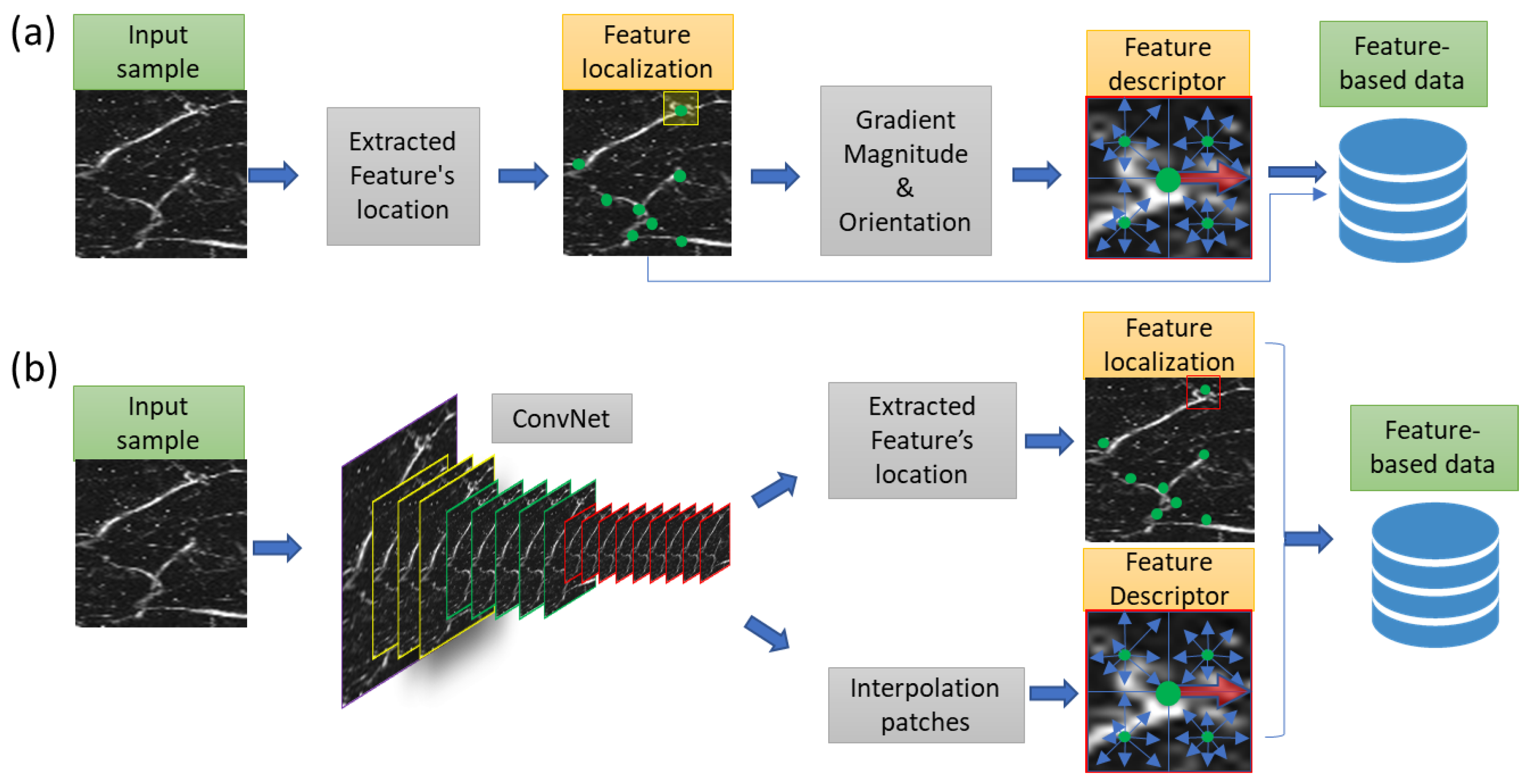
Feature generation (or feature detection) is the process of finding the corners and shapes of objects, which reveals interesting feature objects [60]. Figure 1 shows the step-by-step feature generation process and provides information about two important features: (1) feature localization and (2) feature descriptor. Feature localization is generated from the shape of the object in the image, which shows the difference in intensity between the object and the background. To describe the aiming positions selected as the featured location, the feature values of adjacent pixels surrounding a location are vectorized to identify differences in points that are more interesting than others. This identification process is called the feature descriptor. SIFT, SURF, ORB, and AKAZE are traditional interest feature generation algorithms. As shown in Figure 1a, they follow a single workflow, which locates the feature points first, and then describes the features by vectorizing neighboring pixels. Unfortunately, the performance of these approaches is limited by the hardware performance, storage, and manual work [61]. New solutions are being investigated by applying deep learning algorithms for mosaic imaging, such as convolutional neural networks (CNNs) or GoodPoints [19]. Both methods extract feature localization and feature descriptors from a CNN model, which offers the same information but treats it differently. By generating the feature locations and descriptors simultaneously, the deep interest feature generation shows the possibility of overcoming the time reduction and increasing the calculation efficiency compared to the traditional methods. (Figure 1b).

2.2. Scale Invariant Feature Transform (SIFT)

The SIFT algorithm, introduced by D.G. Lowe [62], was presented as a solution to generate feature descriptions from the patch, even when the rotational and transformational intensity changes during the matching process. The SIFT algorithm consists of four basic processes: (1) estimating an extreme spatial scale by the difference of Gaussian (DoG), (2) extracting features position, (3) assigning orientation on a local patch gradient, and (4) generating a descriptor from features to compute consumption vectors defined for each feature based on feature gradient magnitude and orientation. In the first step, SIFT estimated an extreme spatial scale to find the possible interest points of $Do{G}_{x,y,\sigma }$(in Equation (1)) in image $I$ between Gaussian $G$ in layer $k$ and the first layer. The local difference of the maximum and minimum in DoG was estimated by comparing each sample point to its neighbors in image $I$. Then, the low-contrast points were removed along the edge. Finally, the feature locations (x, y) were extracted $.$

$$Do{G}_{x,y,\sigma }=\left[{\Delta \mathrm{G}}_{x,y}\left(k-1\right)\sigma \right]*I_{x,y}$$

(1)

The feature point was compared to neighboring points with the same scale to choose candidate features $L$. The difference between candidate features and neighboring points was expressed as $\Delta L_x=L_{x+1,y,\sigma }-L_{x-1,y,\sigma }$ and $\Delta L_y=L_{x,y+1,\sigma }-L_{x,y-1,\sigma }$. The descriptor of the point was defined by the magnitude feature point neighborhood $m$ (in Equation (2)) and gradient orientation $\theta$ (in Equation (3)), which provides invariant features.

$$m=\sqrt{\Delta L_x{}^2+\Delta L_y{}^2}$$

(2)

$$\theta ={\tan }^{-1}{\left(\frac{\Delta L_y}{\Delta L_x}\right)}_{}$$

(3)

After obtaining feature information (position, scale, and orientation), we built a descriptor for each feature. A window around the feature point was selected by determining a square region of 16 × 16 pixels around the feature. We divided the region into 4 × 4 sub-regions, which resulted in 16 sub-vectors of 16 pixels each while accessing 128-dimensional vectors, denoted by SIFT128.

2.3. Speeded-Up Robust Features (SURF)

The SURF algorithm was introduced by H. Bay [63] and showed that convolution with the matrix kernel could be accelerated to extract the feature’s location in parallel for different scales. The SURF algorithm has the following four steps: (1) estimating an extreme spatial scale by integral spatial generation, (2) extracting feature position by Hessian detector, (3) assigning orientation on local, and (4) generating a descriptor from features to compute consumption vectors. To adapt to any scale and provide a point $\left(x,y\right)$ in image I, the Hessian block $\mathscr{H}\left(X,\mathsf{\sigma }\right)$ (in Equation (4)) in $\left(x,y\right)$ at scale $\mathsf{\sigma }$ was defined by the approximated Laplacian of Gaussian (LoG) represented as $L_{xx}$, $L_{xy}$, $L_{yy}$.

$$\mathscr{H}\left(X,\sigma \right)=\left[\begin{array}{cc}{L}_{xx}\left(\left(x,y\right),\sigma \right)& L_{xy}\left(\left(x,y\right),\sigma \right)\\ L_{xy}\left(\left(x,y\right),\sigma \right)& L_{yy}\left(\left(x,y\right),\sigma \right)\end{array}\right]$$

(4)

The determinant of the Hessian block was given as $Det\left({\mathscr{H}}_{approx}\right)=D_{xx}*D_{yy}-{\left(0.9D_{xy}\right)}^2$. The use of integral patches made the calculation time independent of the window size, so the SURF was built using a 9 × 9 box with approximations of Gaussian with $\sigma =1.2$. To generate the feature descriptor, the SURF algorithm based on Haar wavelet responses and could be calculated efficiently using integral patches. To determine the orientation, the round cover group of interest was defined with the achievement of orientation-invariant surface rotation in the horizontal direction $dx$ and vertical direction $dy$. Once the wavelet responses were calculated, they were weighed using a Gaussian kernel. After obtaining the orientation of all interest points, a square block covered the interesting point at the center and oriented along the direction. The area was split into a smaller block of 4 × 4 to preserve space information. Thus, each sub-area resulted in a descriptor vector of four dimensions $V=\left(\mathsf{\Sigma }dx, \mathsf{\Sigma }\left|dx\right|,\mathsf{\Sigma }dy, \mathsf{\Sigma }\left|dy\right|\right)$ with all sub-areas and a descriptor vector with 64 dimensions.

2.4. Oriented FAST and Rotated BRIEF (ORB)

Presented by Rublee [3], the ORB has been a rotation-invariant, noise-resistant, and fast algorithm by using a FAST location detector and the BRIEF descriptor. The FAST is a good choice for finding features that match, although it does not measure corners and fails to provide multi-scale features. To obtain scale information, the ORB applied the Harris algorithm to measure the corner at the FAST feature location and then utilized a scaled surface with each stage producing certain FAST features. The orientation of FAST features (in Equation (5)) was produced by the intensity centroid, where $m_{01} \mathrm{and} m_{10}$ represented the moments of a patch ${\mathrm{m}}_{\mathrm{pq}}={\displaystyle \sum }_{x,y}{x}^p*y^q*I\left(x,y\right)$.

$$\theta =a*tan2\left(m_{01},m_{10}\right)$$

(5)

The ORB algorithm used the orientation to direct the original BRIEF descriptor. To patch box $P$, a binary condition $\tau$ was formed by condition variable $p\left(x\right)$ and $p\left(y\right)$ as the intensity of box $P$ at location $\left(x,y\right)$ (in Equation (6)) as:

$$\tau \left(p;x,y\right)=f\left(x\right)=\{\begin{array}{c}1, p\left(x\right)<p\left(y\right)\\ 0, p\left(x\right)\ge p\left(y\right)\end{array}$$

(6)

In each patch, the feature was mapped as a vector T by the statistical method to estimate the point-to-point mapping address. In this study, we chose to limit the map to 10,000 feature points and consider 31 × 31 pixels squared windows for each point in its 5 × 5 sub-windows to set a couple of matches. We used the greedy search method, which repeated the correlation comparison between the next quantity in the mapped vector with a Gaussian distribution around the center of the point until the vector length is 256, and the rotation-aware BRIEF (rBRIEF) feature descriptor is defined.

2.5. Accelerated-KAZE (AKAZE)

Presented by Alcantarilla [64], the AKAZE algorithm was based on a nonlinear scale normalized determinant called fast explicit diffusion (FED). By constructing images of different scales that contain different sublayers, all layers in the AKAZE group showed a similar resolution to the original patch. Thus, the AKAZE algorithm obtains an approximate solution and constructs the cropped pyramid. After nonlinear scale normalization, each patch was computed using the Hessian matrices in different nonlinear scale spatial. This allowed us to classify the maximum value of the detector response in a spatial location. Similar to the SIFT algorithm, the AKAZE algorithm detected feature points by comparing a pixel to its nearby 26 pixels in a 3 × 3 box in its current size and adjacent. By identifying the location features in the center, we found the main directions for the search radius with a sampling step size to ensure that the characteristic rotation is invariant. After obtaining the feature location, scale, and orientation information, we built a feature descriptor by modifying the local difference binary (LDB) to describe the feature descriptors. We selected a patch around the feature location, split it into rectangular grids, and then extracted representative information from each grid cell. Then, the following binary condition $g$ was applied by extracting information from a pair of grid cell $I\left(i\right)$ and $I\left(j\right)$.

$$g\left(I\left(i\right),I(j\right))=\{\begin{array}{c}1, if (I\left(i\right)-I\left(j\right)>0, i\ne j\\ 0, otherwise\end{array}$$

(7)

The AKAZE algorithm chose a binary selection that chooses a group of relevant pairs to model the final descriptor to improve pairing and storage efficiency.

2.6. GoodPoint

Based on the CNN architecture backbone, A.V. Belikov [19] designed unsupervised learning processes for feature detectors and descriptors by following four stages: (1) warping two patches into the same size, (2) extracting feature positions and feature position using a two-headed CNN, (3) calculating descriptor loss as for all interpolated descriptors, (4) the feature location match with the descriptor was used as positive examples from detector training. The detector was trained with a loss function of position map $L_p$ by the summation of the feature’s loss $L_{features}$ and heatmap’s loss $L_{heatmaps}$.

$$L_p=L_{features}+L_{heatmaps}$$

(8)

The descriptor was determined by the loss function of the description map $L_d$ consisting of three components: (1) the loss of ground truth from normalized descriptors $L_{gt}$, (2) the minimized similarity of incorrectly matched pairs of descriptors $L_{unmatch}$, and (3) the minimized difference of randomly sampled descriptors $L_{random}$.

$$L_d=L_{gt}+L_{unmatch}+L_{random}$$

(9)

After generating both features and descriptors, GoodPoint brought pairs of matching points closely matched by coordinates and descriptors as the nearest neighbors. To apply the training process of GoodPoint, we created a patch of 64-pixel squares with PAM samples and then used SIFT as the based-learning method. We named it “PAM dataset,” which has two sub-paths: (1) paired PAM images and (2) listing the top 10 matches of each paired. Gaussian noise with different angles of 10° was applied to the couples. Therefore, the total number of trainable parameters was the same. The descriptor was applied by SoftMax to ensure that the points were not extremely close to each other. Subsequently, normalized tensors were formed on a confidence map interpolated in the feature location.

2.7. Optical-Resolution Photoacoustic Microscopy (PAM)

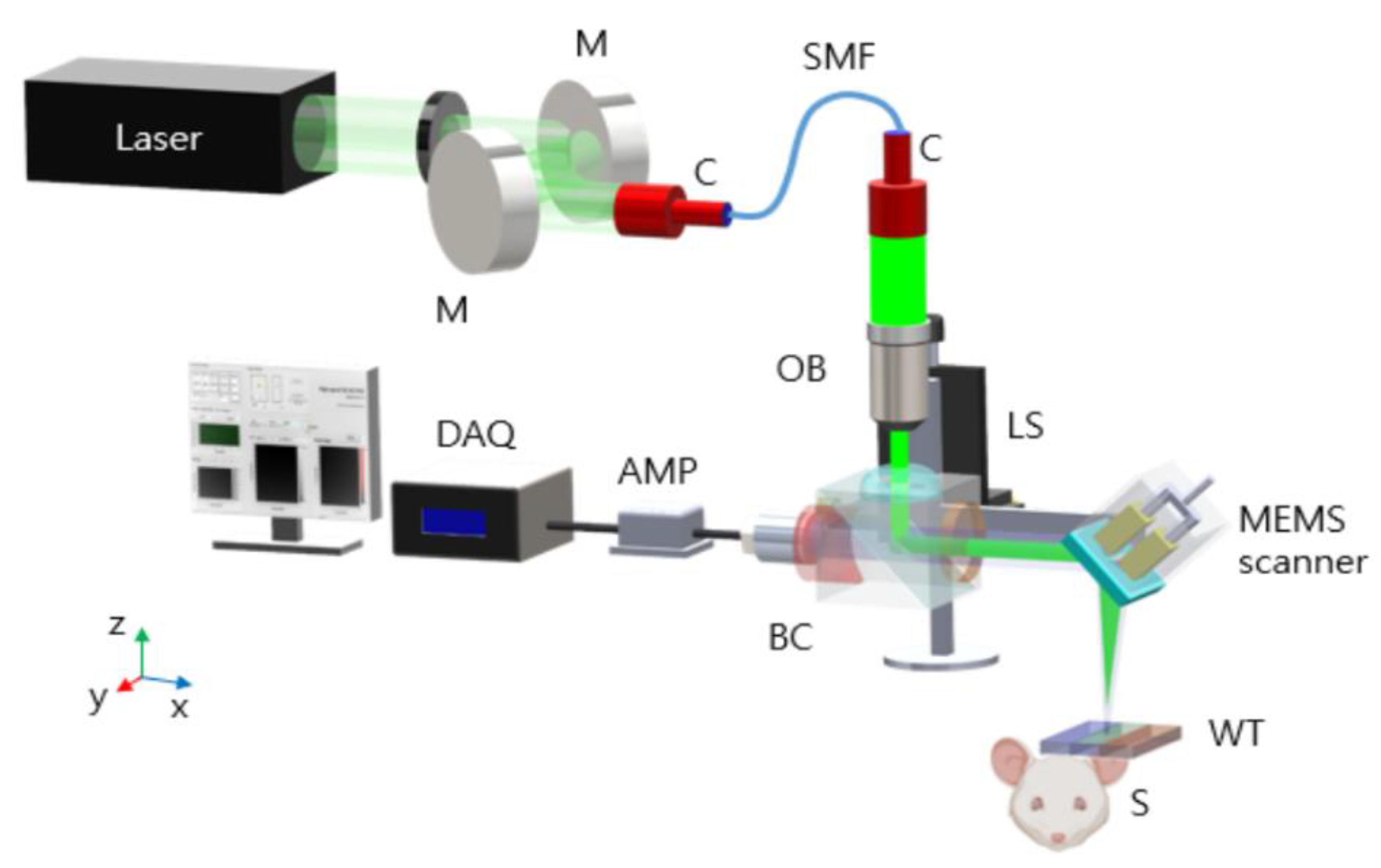
An OR-PAM system was used to acquire all experimental data in this study (Figure 2). The nanosecond pulsed laser (SPOT-10-200-532, Elforlight, Daventry, UK) was controlled by a pulse-width modulation (PWM) channel from the data acquisition board (DAQ) (PCIe-6321, NI Instruments, Austin, TX, USA) to operate the 532 nm centered wavelength laser beam with a pulsed width of 6 ns. The laser beam was collimated to a diameter of 2 mm using an optical fiber (P1-405BPM-FC-1, Thorlabs, NJ, USA). A doublet lens (AC254-060-A, Thorlabs, NJ, USA) formed the focused laser beam. This beam laser, which was reflected 45° by a custom aluminum-coated prism in the beam combiner, was oriented to scan along the x-axis with a single-axis MEMS scanner [54] (OptichoMS-001, OptiCHO Inc., Ltd., Pohang, Korea). To achieve large-area mosaic scanning, two linear stages (L-509, Physik Instrumente (PI), Karlsruhe, Germany) were used for the y-axis and additional x-axis scanning. When the laser beam irradiated the sample, an acoustic wave was generated and passed through the customized beam combiner, which was intensively detected by a commercial transducer (V214-BC-RM, 50 MHz center frequency, Olympus, PA, USA). The acoustic signal was amplified using an amplifier (ZX60-3018G-S+, Mini-Circuit, Brooklyn, NY, USA) with a low-pass crystal filter (CLPFL-0050, 50 MHz, CRYSTEK, Fort Myers, FL, USA). A digitizer (ATS9371, AlazarTech, Pointe-Claire, QC, Canada) converted the acoustic signal to digital values. The OR-PAM scanning driver and reconstruction process were operated using the LabVIEW program (National Instruments, Austin, TX, USA). The measured lateral and axial resolutions were 12 μm and 27 μm, respectively [41]. The size of each PAM image patch was 30 mm/500 pixels on the y-axis and 5 mm/140 pixels on the x-axis.

2.8. Animal Preparing

The experimental animal procedures followed the laboratory animal protocols admitted by the institutional animal care and use committee of Chonnam National University Hwasun Hospital. One healthy eight-week-old male BALB/c mouse, weighing ~20 g, was purchased from Orient Bio (Iksan, Korea). To anesthetize the mouse, a cocktail of ketamine and xylazine (80:12) was applied. After removing the downy hair with the hair removing gel, the mouse was placed on a fixed holder with a temperature maintaining bed using an isoflurane system (Luna Vaporiser, NorVap International Ltd., Barrowford, UK) while scanning in vivo observations. The energy of the illuminated laser pulse on the mouse skin was approximately $5 \mathrm{mJ}/{\mathrm{cm}}^2$ below the ANSI safety limit of $\left(20 \mathrm{mJ}/{\mathrm{cm}}^2\right)$.

2.9. Mosaic PAM Imaging Process

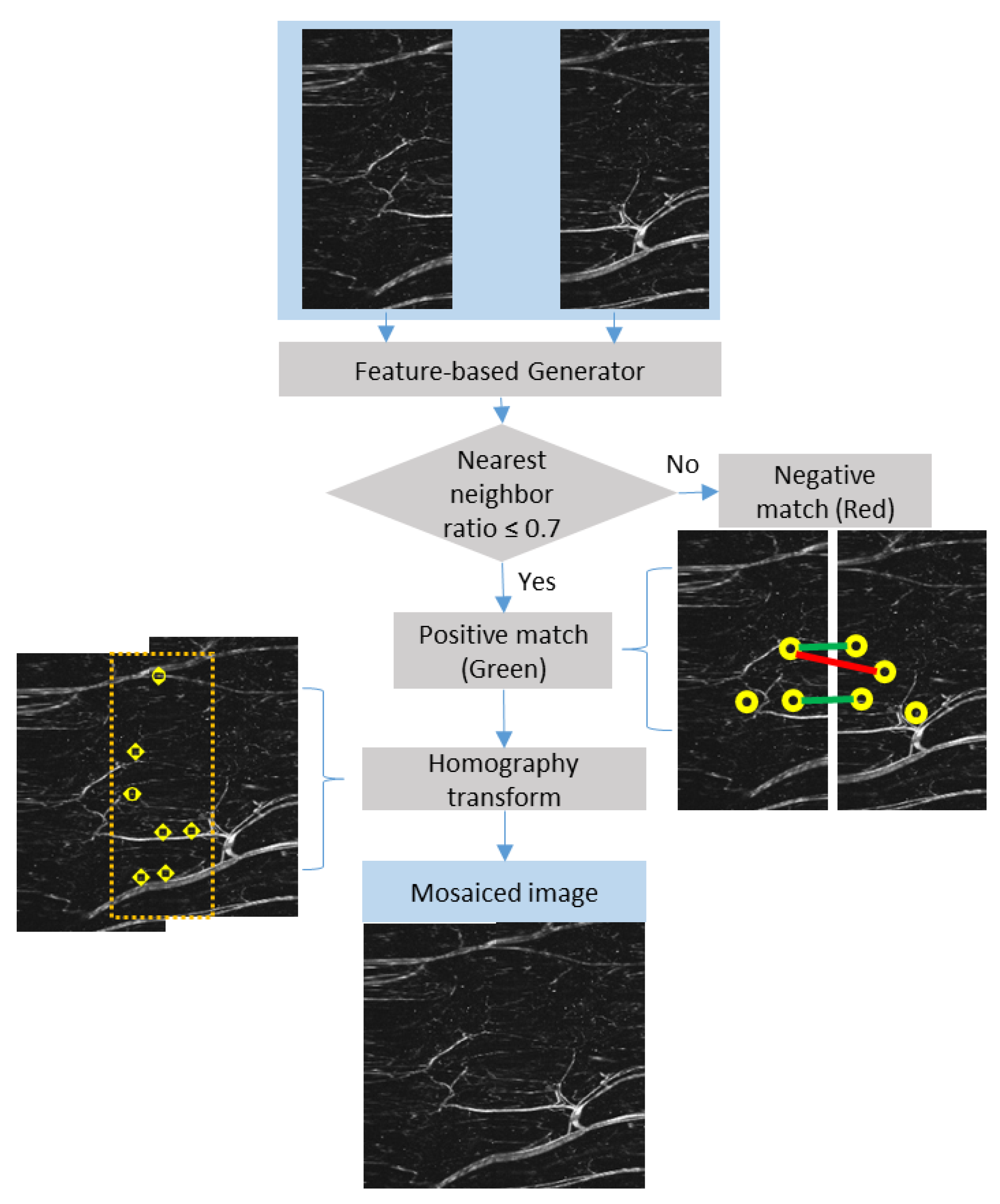
The mosaic image generation is shown in Figure 3. This process followed three steps: (1) selecting good matching points by the nearest neighbor distance decision, (2) aligning feature couples using the RANSAC algorithm [65], and (3) connecting the matching area using the homograph transform. First, we used a feature-based generator to extract the feature information (location and vector descriptors). Each feature was linked together as matches using the k-nearest neighbor algorithm by a binary decision to find approximate nearest neighbors. This step removed negative matches and maintained the positive ones chosen by the NNDR value below 0.7 [62]. To minimize the matching error, the RANSAC algorithm was applied iteratively to obtain the largest matches adequate for the merging process. These inlier matches had been used to estimate the space transform between two duplicated areas of PAM images. The homograph matrix $H$ could be presented as the transfer from $\mathrm{X}$ coordinate to $\mathrm{X}\prime$ of two sub-images:

$$\mathrm{X}\prime =H\mathrm{X}$$

(10)

After obtaining the homograph, two sub-images were selected: the target patch and the source patch. In this process, we decided that the source patch has an overlap area on the right of the patch as the current space. Therefore, the target patch was warped from another direction to the current space as defined by the previous step. Because these patches were recorded in the same scan, the difference in contrast and brightness had no influence.

2.10. Computing System

The specifications of the computing system were as follows: Processor Intel^® Core ™ i9-10900K @ 3.70 GHz (Intel Corp., City of Santa Clara, CA, USA) with 64 GB of RAM (Samsung Corp., Suwon, Korea). The program was written in Ubuntu 20.04 LTS 64-bit, using Python 3 as a compiler with basic image processing and feature generation of the OpenCV 3.4 library. For the deep feature architecture, we used the PyTorch framework.

2.11. Performance Evaluation

To compare the performance of different mosaic imaging processes, we chose four factors that directly affected our decision: (1) processing time, (2) number of matching points, (3) good matching ratio, and (4) matching efficiency.

(1)

Processing time: Using system resources directly, we estimated the time consumed to complete the feature generation process. The processing time began from algorithm detection until the matching process was completed. By estimating the processing time, we could determine which methods were lighter and required few resources to process while maintaining the same performance.

(2)

Number of matching points: By maintaining the same conditions for the mosaic imaging generator ($\mathrm{NNDR}\ge 0.7$), each feature generation method provided a different number of matching points. The number of matching points (matrix transformation conditions) should be as more than four as possible. More matching points mean more chances for a high-quality mosaicking process.

(3)

Good matching ratio (GMR): By removing negative matching points ($\mathrm{NNDR}<0.7$) and maintaining positive matching points ($\mathrm{NNDR}\ge 0.7$), we estimated the accuracy of the feature generation methods.

$$\mathrm{GMR}=\frac{\mathrm{Number}\mathrm{of}\mathrm{positive}\mathrm{matching}\mathrm{points}}{\mathrm{Total}\mathrm{of}\mathrm{matches}}\times 100(\%)$$

(11)

(4)

Matching efficiency: Matching efficiency shows the number of positive matching points in one millisecond. In this way, we estimated algorithms to reduce the time consumed while maintaining similar performance.

$$\mathrm{Matching}\mathrm{efficiency}=\frac{\mathrm{Number}\mathrm{of}\mathrm{positive}\mathrm{matches}}{\mathrm{Processing}\mathrm{Time}}$$

(12)

2.12. Dataset Preparing

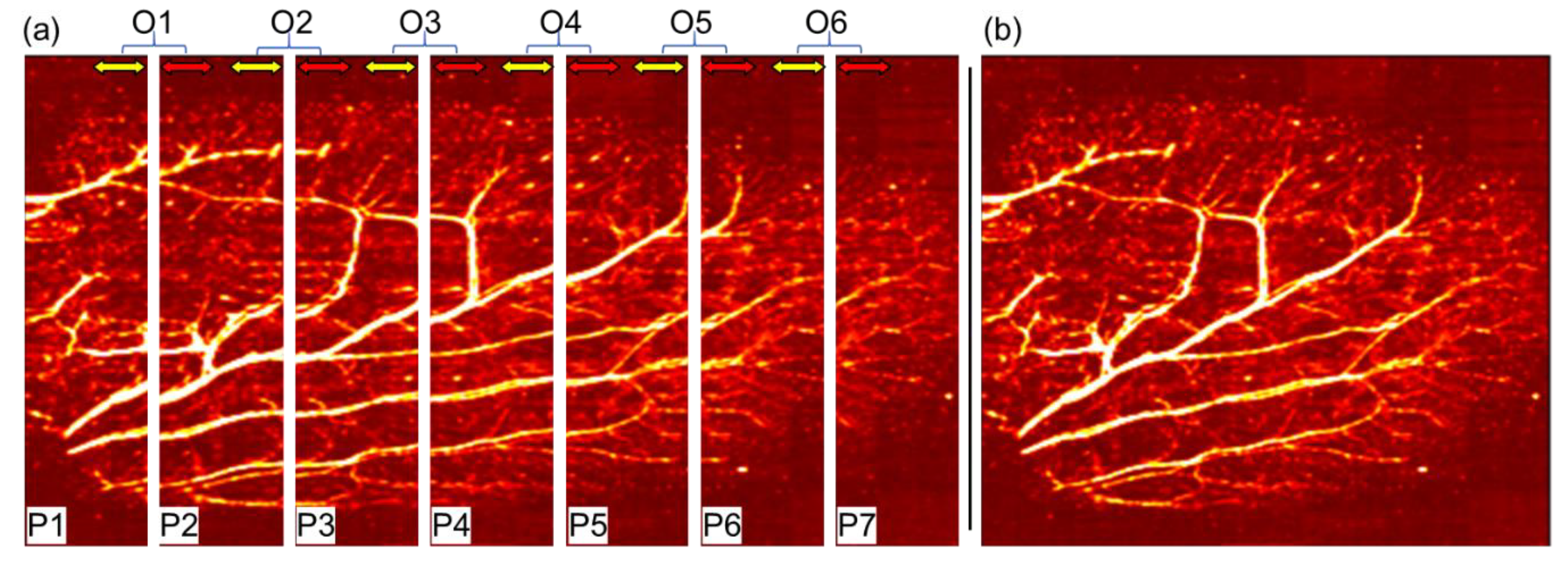
The dataset was reconstructed to the maximum amplitude projection (MAP) from the OR-PAM scanning of the mouse ear. The dataset for training included 7-volume patches shown as the different areas on the mouse ear with the duplicated area (from 5% to 80% area of each patch, Figure 4).

For testing GoodPoint, we prepared the MS-COCO dataset [66] and FIRE dataset [67] as the pre-trained dataset to ensure that the amount of data files was large enough for training and closest to vessel shapes. We used 40 OR-PAM patches with $\pm 10°$ angle with salt-and-pepper noise $\sigma =0.05$ and created a dataset with SIFT matching as fine-tuned data to fit with PAM general properties. The training was conducted using AdamW [68] as an optimization algorithm with an initial learning rate of 0.0005, and all other parameters were set to default values [17].

3. Results

3.1. Performance Comparison

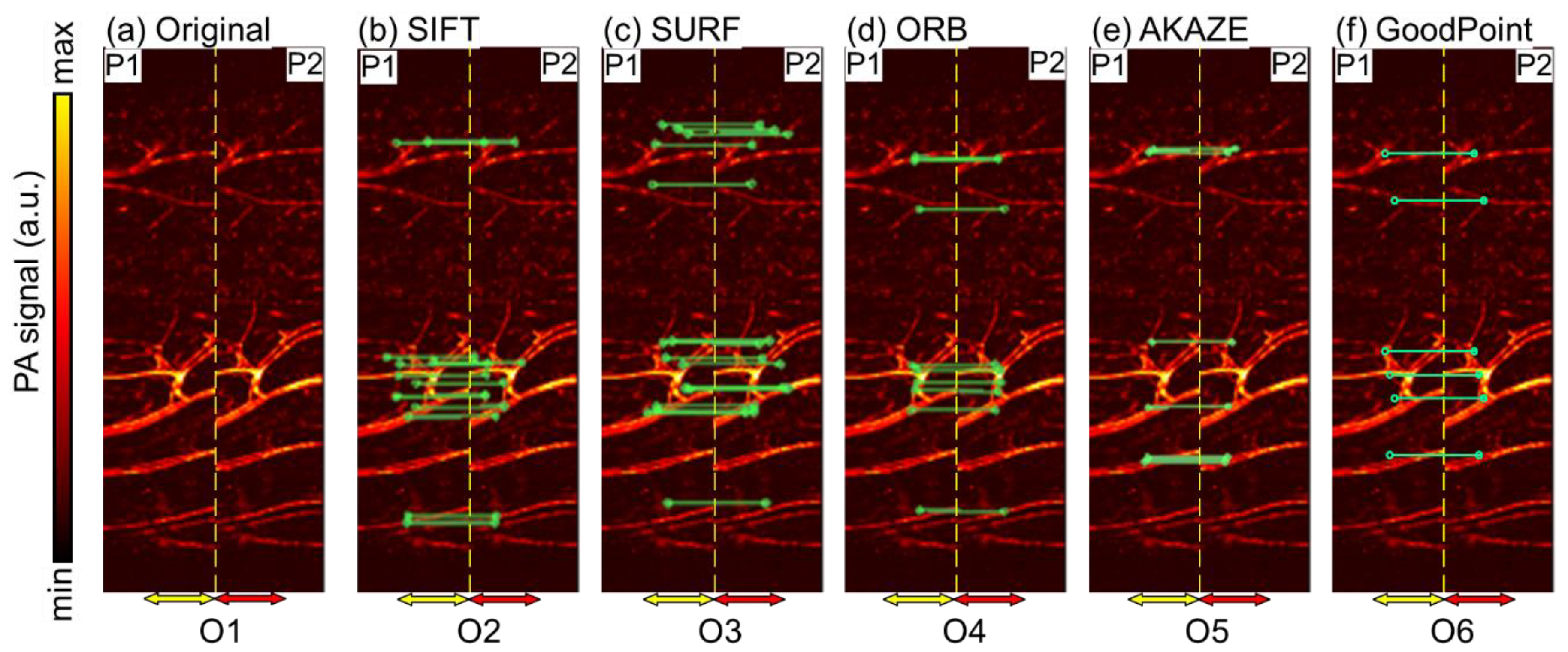
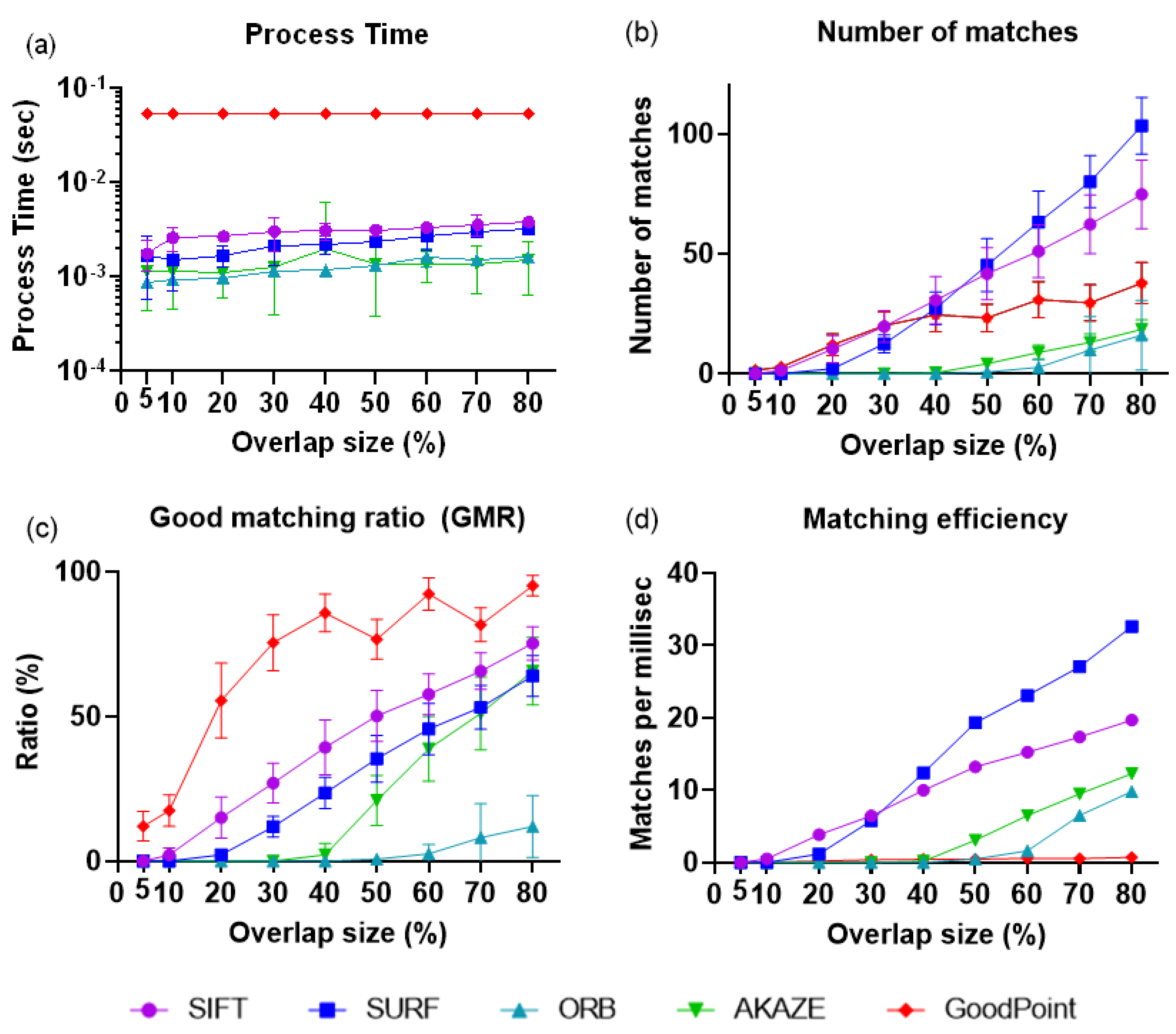
As shown in Figure 5, the feature extraction and matching in two neared PAM image patches were conducted by SIFT, SURF, ORB, AKAZE, and GoodPoint by controlling the overlapping area from 5% to 80%. The matched condition, in which the NNDR ratio equaled 0.7, is indicted by the green lines in Figure 5b–f at different feature matching algorithms. To evaluate the performance, we calculated the stitching processing time for the two PAM MAP image patches, as shown in Figure 6a. ORB (1.177 ms) and AKAZE (1.273 ms) were the fastest algorithms in replying to the results. Slower than these, SURF required 2.148 ms to generate and match. SIFT took an average of 3.045 ms; thus, it was the slowest traditional algorithm. GoodPoint took 5.294 ms to load the trained model and conduct the process. Next, by estimating the number of matching points, feature generation methods generally showed an increasing number of matching points depending on the change in the overlapping range, as shown in Figure 6b. When the overlapping area was below 10%, none of the methods generated sufficient matches for the mosaicking process. SIFT, SURF, and GoodPoint showed one or three matches, and both ORB and AKAZE did not generate any matching points. In the range from 10% to 40%, SIFT and GoodPoint could generate an average of 12 and 20 matching points, respectively, while SURF only showed two matching points at a 20% overlapping range and 12 matching points at a 30% overlapping range. In the upper 40% duplicated overlapping area, SURF showed the number of matching points equal to SIFT (35 matching points) at a 45% overlapping area, when GoodPoint generated 24 matching points. At 50% duplicated overlapping area, ORB and AKAZE generated approximately four matching points. To obtain more than four matching points, the ORB needed an overlapping range of more than 65%. Figure 6c showed the GMR values for different overlapping areas. GoodPoint showed good opportunity with 55.4 matching points and passed the NNDR condition at the 20% overlapping range. The GMR of SIFT and SURF linearly increased from 2% at a 10% overlapping area to 75% (SIFT) and 65.6% (SURF) at an 80% overlapping area. AKAZE showed a GMR value of 2% at a 40% overlapping area and a GMR value of 65.6% at an 80% overlapping area. ORB showed the lowest GMR value of 1.63% at a 60% overlapping area and a slight increase in the GRM value of 9.8% at an 80% overlapping area. To clarify the goals, we estimated the matching efficiency (Figure 6d), which indicated the number of accepted matches by time to compare the efficiency among all implemented algorithms. GoodPoint was too slow, so its generator only showed 0.7 matching points per 1 ms. At a 30% overlapping range, SIFT and SURF enabled the generation of 6.46 and 5.78 matching points per 1 ms, respectively. AKAZE could generate 6.46 matching points (at a 60% overlapping range), and ORB could generate 6.51 matching points (at a 70% overlapping range) per 1 ms.

3.2. Whole Mosaic OR-PAM Image Generation

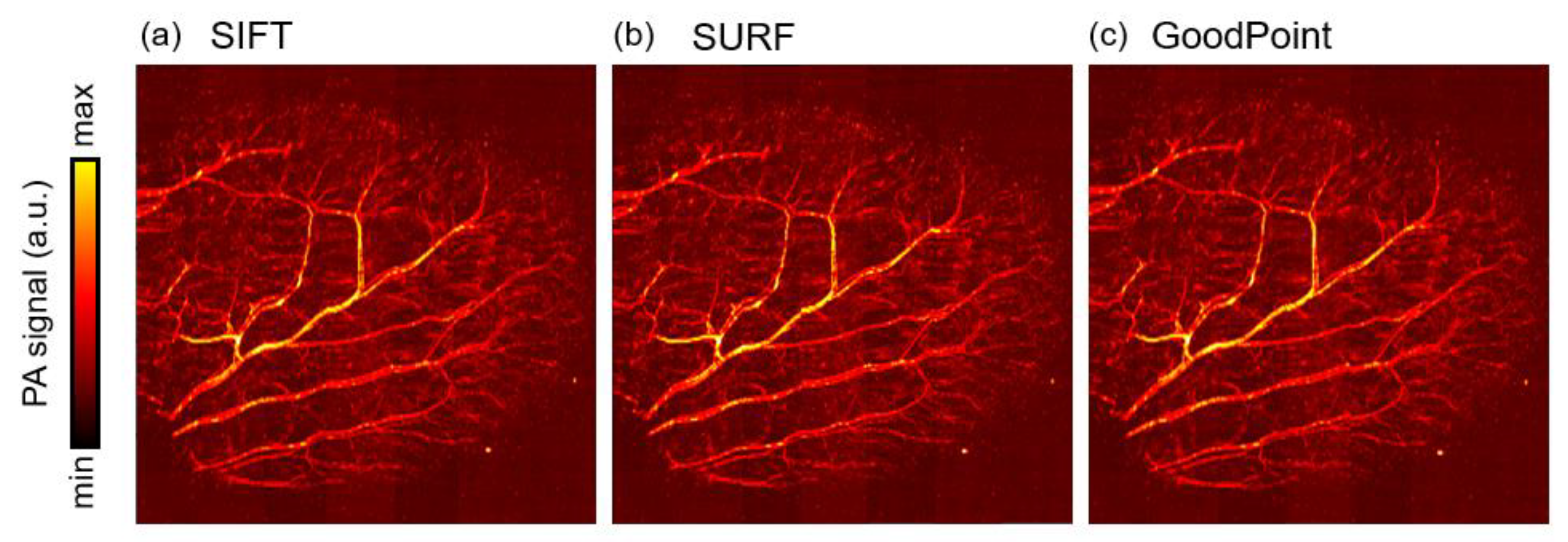
Using the feature generation algorithms, we applied mosaic processing to our custom PAM system to reconstruct a wide-field PAM MAP image of the mouse ear. As shown in Figure 4a, the overlapping areas among the small imaging patches were smaller than 20%. Therefore, based on our analysis results, only the SIFT, SURF, and GoodPoint methods were available and could be used to complete the mosaic imaging process. In Figure 4b, we manually merged all PAM imaging patches by removing non-linear areas and cutting the overlapping range. Then, we assembled the imaging patches manually. In Figure 7a–c, we used feature generation algorithms as the marked border to automatically remove non-linear areas and merge duplicated patches by homography estimation. SIFT, SURF, and GoodPoint successfully generated mosaic 30 × 30 mm PAM MAP images.

4. Discussion

We compared the performance of feature generation algorithms for PAM images in Section 3.1 and applied these algorithms with our custom experiment setup in Section 3.2. Comparing the processing time in Figure 6a, the traditional feature generation algorithms were 100 times faster than the deep learning feature generation algorithm (GoodPoint). The GoodPoint algorithm did not optimize the decoder layers to extract feature points in a short time (approximately 300 ms). The traditional feature generation algorithms required a focused window of feature points in SIFT and SURF or binary mapping in ORB and AKAZE. The traditional feature generation methods showed similar processing times because the computer system supported Intel Distribution for Python [69]. So, the feature generation algorithms of SIFT (approximately 2.6 ms), SURF (approximately 1.5 ms), ORB (approximately 1.1 ms), and AKAZE (approximately 1.2 ms) consumed less processing time when merging small mosaicking patches’ size.

By analyzing Figure 6b, GoodPoint ’s matching points showed a similar quantality of SIFT and SURF when the overlapping range was smaller than 45% because we used our OR-PAM projection dataset created by the SIFT algorithm. ORB and AKAZE did not generate sufficient feature matching when the overlapping range was smaller than 50%. Above the 50% overlapping range, the SURF algorithm extracted most matching points and increased 1.5 times faster by each step with a 10% overlapping increment range. In this range, the GoodPoint algorithm did not generate noticeably matching points. ORB and AKAZE slowly increased from less than four matching points but did not generate enough matching points for decision (less than 11 matching points when the overlapping range was 80%).

According to Figure 6c, GoodPoint was the best choice when you wanted to store similar matching points such as SIFT and SURF and maintain similar good matching points (GoodPoint showed 24 matching points, but 11 matching points did not pass the NNDR condition). At less than a 40% overlapping area, SIFT and SURF only maintained less than 40% and 25% good matching points, respectively. This means that most of the matching points were removed. More than 88% of the ORB matching points did not pass the NNDR condition. Therefore, the ORB algorithm was not a good algorithm for mosaic PAM image generation. AKAZE was the better choice than ORB when the overlapping area was larger than 50%. However, the ORB and AKAZE algorithms were not suitable for generating the features in PAM images, which maintained mosaicking patches with less than a 10% overlapping range.

By analyzing the matching efficiency in Figure 6d, we could observe that the SIFT generated more matching points than the other methods when the overlapping range was below 30%. Although GoodPoint generated the same matching points as SIFT or SURF in that range because the processing time of GoodPoint was 100 times that of SIFT and SURF, the matching efficiency value of GoodPoint was the lowest. In addition, in a custom experimental setup, GoodPoint was slow enough to have a negative impact on a real-time system.

To apply feature generation algorithms with our custom OR-PAM setup, the algorithms were coded in Python executable and were used as LabVIEW’s custom library. In Section 3.2, the mosaic images of SIFT, SURF, and GoodPoint showed similarities when merging six patches automatically. Compared to manual mosaicking in Figure 4b, the mosaic projection by SIFT showed acceptable scaling. SURF and GoodPoint showed that a few unmatching vessels were not better than manual mosaicking. Because the GoodPoint processing time was slow (approximately 500 ms for each mosaicking process), the total scanning process was slow. SIFT and SURF, which were optimized using the OpenCV library and Intel Distribution for Python, proved to be good solutions with our current experimental computer configuration.

5. Conclusions

In this study, we compared and analyzed the performance of various feature-generation algorithms for mosaic PAM images. In short, traditional feature generation algorithms were stable and easy to apply. However, owing to the limitations of computing power, traditional feature generation algorithms require computing systems up-gradation to increase efficiency. Contrary to our expectations, the deep learning feature generation algorithms did not overperform traditional algorithms when they required a pre-training dataset that should be such as an object’s properties and consumed more processing time than that required by traditional algorithms. These were the disadvantages of applying deep learning feature generation algorithms. However, the advantage of deep learning generation algorithms was that they could be modified to focus more on the best matching ratio, make better decisions, and spend less computing power to generate matching points. These results were used and chosen as customized choices for the mosaicking process. Finally, we updated our PAM reconstruction program using mosaic processing as the default option. Further, SIFT, SURF, and GoodPoint were added to the optional functions. We confirmed that the program could be used safely without interference during operation.

References

- Yun Tian, G.; Gledhill, D.; Taylor, D. Comprehensive Interest Points Based Imaging Mosaic. Pattern Recognit. Lett. 2003, 24, 1171–1179. [Google Scholar] [CrossRef]
- Can, A.; Stewart, C.V.; Roysam, B.; Tanenbaum, H.L. A Feature-Based Technique for Joint, Linear Estimation of High-Order Image-to-Mosaic Transformations: Mosaicing the Curved Human Retina. IEEE Trans. Pattern Anal. Mach. Intell. 2002, 24, 412–419. [Google Scholar] [CrossRef]
- Battiato, S.; Di Blasi, G.; Farinella, G.M.; Gallo, G. Digital Mosaic Frameworks-An Overview. Comput. Graph. Forum 2007, 26, 794–812. [Google Scholar] [CrossRef] [Green Version]
- Li, X.; Feng, R.; Guan, X.; Shen, H.; Zhang, L. Remote Sensing Image Mosaicking: Achievements and Challenges. IEEE Geosci. Remote Sens. Mag. 2019, 7, 8–22. [Google Scholar] [CrossRef]
- Katz, D.S.; Berriman, G.B.; Mann, R.G. Collaborative Astronomical Image Mosaics. arXiv 2010, arXiv:10115294. [Google Scholar]
- Wu, M.; Yang, C.; Song, X.; Hoffmann, W.C.; Huang, W.; Niu, Z.; Wang, C.; Li, W. Evaluation of Orthomosics and Digital Surface Models Derived from Aerial Imagery for Crop Type Mapping. Remote Sens. 2017, 9, 239. [Google Scholar] [CrossRef] [Green Version]
- Turner, D.; Lucieer, A.; Watson, C. An Automated Technique for Generating Georectified Mosaics from Ultra-High Resolution Unmanned Aerial Vehicle (UAV) Imagery, Based on Structure from Motion (SfM) Point Clouds. Remote Sens. 2012, 4, 1392–1410. [Google Scholar] [CrossRef] [Green Version]
- Zhang, W.; Li, X.; Yu, J.; Kumar, M.; Mao, Y. Remote Sensing Image Mosaic Technology Based on SURF Algorithm in Agriculture. EURASIP J. Image Video Process. 2018, 2018, 1–9. [Google Scholar] [CrossRef]
- Li, Z.; Isler, V. Large Scale Image Mosaic Construction for Agricultural Applications. IEEE Robot. Autom. Lett. 2016, 1, 295–302. [Google Scholar] [CrossRef]
- Díaz, M.; de Moura, J.; Novo, J.; Ortega, M. Automatic Wide Field Registration and Mosaicking of OCTA Images Using Vascularity Information. Procedia Comput. Sci. 2019, 159, 505–513. [Google Scholar] [CrossRef]
- Chow, S.K.; Hakozaki, H.; Price, D.L.; MacLean, N.a.B.; Deerinck, T.J.; Bouwer, J.C.; Martone, M.E.; Peltier, S.T.; Ellisman, M.H. Automated Microscopy System for Mosaic Acquisition and Processing. J. Microsc. 2006, 222, 76–84. [Google Scholar] [CrossRef]
- Mokso, R. X-Ray Mosaic Nanotomography of Large Microorganisms. J. Struct. Biol. 2012, 177, 233–238. [Google Scholar] [CrossRef]
- Piccinini, F.; Bevilacqua, A.; Lucarelli, E. Automated Image Mosaics by Non-Automated Light Microscopes: The MicroMos Software Tool: Automated Image Mosaics by Non-Automated Light Microscopes. J. Microsc. 2013, 252, 226–250. [Google Scholar] [CrossRef]
- Harris, C.; Stephens, M. A Combined Corner and Edge Detector. In Alvey Vision Conference; Alvey Vision Club: Manchester, UK, 1988; pp. 23.1–23.6. [Google Scholar]
- Rosten, E.; Drummond, T. Machine Learning for High-Speed Corner Detection. In Computer Vision–ECCV 2006; Leonardis, A., Bischof, H., Pinz, A., Eds.; Springer: Berlin/Heidelberg, Germany, 2006; pp. 430–443. [Google Scholar]
- Hutchison, D.; Kanade, T.; Kittler, J.; Kleinberg, J.M.; Mattern, F.; Mitchell, J.C.; Naor, M.; Nierstrasz, O.; Pandu Rangan, C.; Steffen, B.; et al. BRIEF: Binary Robust Independent Elementary Features. In Computer Vision–ECCV 2010; Daniilidis, K., Maragos, P., Paragios, N., Eds.; Lecture Notes in Computer Science; Springer: Berlin/Heidelberg, Germany, 2010; Volume 6314, pp. 778–792. ISBN 978-3-642-15560-4. [Google Scholar]
- Zhao, H.; Chen, N.; Li, T.; Zhang, J.; Lin, R.; Gong, X.; Song, L.; Liu, Z.; Liu, C.; Hidalgo, F.; et al. ORB: An Efficient Alternative to SIFT or SURF. Int. J. Comput. Vis. 2019, 4, 4162–4169. [Google Scholar] [CrossRef]
- Kalms, L.; Mohamed, K.; Göhringer, D. Accelerated Embedded AKAZE Feature Detection Algorithm on FPGA. In Proceedings of the 8th International Symposium on Highly Efficient Accelerators and Reconfigurable Technologies, Bochum, Germany, 7–9 June 2017. [Google Scholar] [CrossRef]
- Belikov, A.V.; Potapov, A.S.; Yashchenko, A.V. Goodpoint: Unsupervised Learning of Key Point Detection and Description. Sci. Tech. J. Inf. Technol. Mech. Opt. 2021, 21, 92–101. [Google Scholar] [CrossRef]
- Zhu, H.; Wen, X.; Zhang, F.; Wang, X.; Wang, G. Homography Estimation Based on Order-Preserving Constraint and Similarity Measurement. IEEE Access 2018, 6, 28680–28690. [Google Scholar] [CrossRef]
- Wang, L.; Traub, J.; Heining, S.M.; Benhimane, S.; Euler, E.; Graumann, R.; Navab, N. Long Bone X-Ray Image Stitching Using C-Arm Motion Estimation. Inform. Aktuell 2009, 2009, 202–206. [Google Scholar] [CrossRef] [Green Version]
- Meine, H.; Hering, A. Efficient Prealignment of CT Scans for Registration through a Bodypart Regressor. arXiv 2019, arXiv:190908898. [Google Scholar]
- Shilling, R.Z.; Brummer, M.E.; Mewes, K. Merging Multiple Stacks MRI into a Single Data Volume. In Proceedings of the 3rd IEEE International Symposium on Biomedical Imaging: Nano to Macro, Arlington, VA, USA, 6–9 April 2006; pp. 1012–1015. [Google Scholar]
- Townsend, D.W. Combined Positron Emission Tomography-Computed Tomography: The Historical Perspective. Semin. Ultrasound CT MRI 2008, 29, 232–235. [Google Scholar] [CrossRef] [Green Version]
- Yaniv, Z.; Joskowicz, L. Long Bone Panoramas from Fluoroscopic X-Ray Images. IEEE Trans. Med. Imaging 2004, 23, 26–35. [Google Scholar] [CrossRef]
- Bakar, S.A.; Jiang, X.; Gui, X.; Li, G.; Li, Z. Image Stitching for Chest Digital Radiography Using the SIFT and SURF Feature Extraction by RANSAC Algorithm. J. Phys. Conf. Ser. 2020, 1624. [Google Scholar] [CrossRef]
- Ni, D.; Chui, Y.P.; Qu, Y.; Yang, X.; Qin, J.; Wong, T.-T.; Ho, S.S.H.; Heng, P.A. Reconstruction of Volumetric Ultrasound Panorama Based on Improved 3D SIFT. Comput. Med. Imaging Graph. 2009, 33, 559–566. [Google Scholar] [CrossRef]
- Seo, J.-H.; Yang, S.; Kang, M.-S.; Her, N.-G.; Nam, D.-H.; Choi, J.-H.; Kim, M.H. Automated Stitching of Microscope Images of Fluorescence in Cells with Minimal Overlap. Micron 2019, 126, 102718. [Google Scholar] [CrossRef]
- Jain, M.; Rajadhyaksha, M.; Nehal, K. Implementation of Fluorescence Confocal Mosaicking Microscopy by “Early Adopter” Mohs Surgeons and Dermatologists: Recent Progress. J. Biomed. Opt. 2017, 22, 17. [Google Scholar] [CrossRef] [PubMed] [Green Version]
- Zhang, H.F.; Maslov, K.; Stoica, G.; Wang, L.V. Functional Photoacoustic Microscopy for High-Resolution and Noninvasive in Vivo Imaging. Nat. Biotechnol. 2006, 24, 848–851. [Google Scholar] [CrossRef] [PubMed]
- Lee, C.; Kim, J.Y.; Kim, C. Recent Progress on Photoacoustic Imaging Enhanced with Microelectromechanical Systems (MEMS) Technologies. Micromachines 2018, 9, 584. [Google Scholar] [CrossRef] [Green Version]
- Jung, D.; Park, S.; Lee, C.; Kim, H. Recent Progress on Near-Infrared Photoacoustic Imaging: Imaging Modality and Organic Semiconducting Agents. Polymers 2019, 11, 1693. [Google Scholar] [CrossRef] [Green Version]
- Jeon, S.; Kim, J.; Lee, D.; Baik, J.W.; Kim, C. Review on Practical Photoacoustic Microscopy. Photoacoustics 2019, 15, 100141. [Google Scholar] [CrossRef]
- Strohm, E.M.; Moore, M.J.; Kolios, M.C. Single Cell Photoacoustic Microscopy: A Review. IEEE J. Sel. Top. Quantum Electron. 2016, 22, 137–151. [Google Scholar] [CrossRef]
- Hai, P.; Imai, T.; Xu, S.; Zhang, R.; Aft, R.L.; Zou, J.; Wang, L.V. High-Throughput, Label-Free, Single-Cell Photoacoustic Microscopy of Intratumoral Metabolic Heterogeneity. Nat. Biomed. Eng. 2019, 3, 381–391. [Google Scholar] [CrossRef]
- Han, J.; Yang, P.; Tang, S. Local Acoustic Field Enhancement of Single Cell Photoacoustic Signal Detection Based on Metamaterial Structure. AIP Adv. 2019, 9, 095064. [Google Scholar] [CrossRef] [Green Version]
- Lee, C.; Jeon, M.; Jeon, M.Y.; Kim, J.; Kim, C. In Vitro Photoacoustic Measurement of Hemoglobin Oxygen Saturation Using a Single Pulsed Broadband Supercontinuum Laser Source. Appl. Opt. 2014, 53, 3884–3889. [Google Scholar] [CrossRef] [PubMed]
- Zhou, H.-C.; Chen, N.; Zhao, H.; Yin, T.; Zhang, J.; Zheng, W.; Song, L.; Liu, C.; Zheng, R. Optical-Resolution Photoacoustic Microscopy for Monitoring Vascular Normalization during Anti-Angiogenic Therapy. Photoacoustics 2019, 15, 100143. [Google Scholar] [CrossRef]
- Zhao, J.; Zhao, Q.; Lin, R.; Meng, J. A Microvascular Image Analysis Method for Optical-Resolution Photoacoustic Microscopy. J. Innov. Opt. Health Sci. 2020, 13, 2050019. [Google Scholar] [CrossRef]
- Mai, T.T.; Vo, M.-C.; Chu, T.-H.; Kim, J.Y.; Kim, C.; Lee, J.-J.; Jung, S.-H.; Lee, C. Pilot Study: Quantitative Photoacoustic Evaluation of Peripheral Vascular Dynamics Induced by Carfilzomib In Vivo. Sensors 2021, 21, 836. [Google Scholar] [CrossRef]
- Mai, T.T.; Yoo, S.W.; Park, S.; Kim, J.Y.; Choi, K.-H.; Kim, C.; Kwon, S.Y.; Min, J.-J.; Lee, C. In Vivo Quantitative Vasculature Segmentation and Assessment for Photodynamic Therapy Process Monitoring Using Photoacoustic Microscopy. Sensors 2021, 21, 1776. [Google Scholar] [CrossRef]
- Wong, T.T.W.; Zhang, R.; Zhang, C.; Hsu, H.-C.; Maslov, K.I.; Wang, L.; Shi, J.; Chen, R.; Shung, K.K.; Zhou, Q.; et al. Label-Free Automated Three-Dimensional Imaging of Whole Organs by Microtomy-Assisted Photoacoustic Microscopy. Nat. Commun. 2017, 8, 1–8. [Google Scholar] [CrossRef]
- Park, E.-Y.; Lee, D.; Lee, C.; Kim, C. Non-Ionizing Label-Free Photoacoustic Imaging of Bones. IEEE Access 2020, 8, 160915–160920. [Google Scholar] [CrossRef]
- Bi, R.; Ma, Q.; Mo, H.; Olivo, M.; Pu, Y. Optical-resolution photoacoustic microscopy of brain vascular imaging in small animal tumor model using nanosecond solid-state laser. In Neurophotonics and Biomedical Spectroscopy; Elsevier: Amsterdam, The Netherlands, 2018; pp. 159–187. ISBN 978-0-323-48067-3. [Google Scholar]
- Yao, J.; Wang, L.; Yang, J.-M.; Maslov, K.I.; Wong, T.T.W.; Li, L.; Huang, C.-H.; Zou, J.; Wang, L.V. High-Speed Label-Free Functional Photoacoustic Microscopy of Mouse Brain in Action. Nat. Methods 2015, 12, 407–410. [Google Scholar] [CrossRef]
- Kim, J.; Kim, J.Y.; Jeon, S.; Baik, J.W.; Cho, S.H.; Kim, C. Super-Resolution Localization Photoacoustic Microscopy Using Intrinsic Red Blood Cells as Contrast Absorbers. Light Sci. Appl. 2019, 8, 103. [Google Scholar] [CrossRef]
- Yeh, C.; Hu, S.; Maslov, K.; Wang, L.V. Photoacoustic Microscopy of Blood Pulse Wave. J. Biomed. Opt. 2012, 17, 070504. [Google Scholar] [CrossRef] [PubMed] [Green Version]
- Liu, W.; Shcherbakova, D.M.; Kurupassery, N.; Li, Y.; Zhou, Q.; Verkhusha, V.V.; Yao, J. Quad-Mode Functional and Molecular Photoacoustic Microscopy. Sci. Rep. 2018, 8, 11123. [Google Scholar] [CrossRef] [PubMed]
- Yao, J.; Wang, L.V. Recent Progress in Photoacoustic Molecular Imaging. Curr. Opin. Chem. Biol. 2018, 45, 104–112. [Google Scholar] [CrossRef] [PubMed] [Green Version]
- Yoo, S.W.; Jung, D.; Min, J.-J.; Kim, H.; Lee, C. Biodegradable Contrast Agents for Photoacoustic Imaging. Appl. Sci. 2018, 8, 1567. [Google Scholar] [CrossRef] [Green Version]
- Park, B.; Lee, K.M.; Park, S.; Yun, M.; Choi, H.-J.; Kim, J.; Lee, C.; Kim, H.; Kim, C. Deep Tissue Photoacoustic Imaging of Nickel(II) Dithiolene-Containing Polymeric Nanoparticles in the Second near-Infrared Window. Theranostics 2020, 10, 2509–2521. [Google Scholar] [CrossRef]
- Lee, C.; Kwon, W.; Beack, S.; Lee, D.; Park, Y.; Kim, H.; Hahn, S.K.; Rhee, S.-W.; Kim, C. Biodegradable Nitrogen-Doped Carbon Nanodots for Non-Invasive Photoacoustic Imaging and Photothermal Therapy. Theranostics 2016, 6, 2196–2208. [Google Scholar] [CrossRef] [Green Version]
- Yao, J.; Wang, L.; Yang, J.-M.; Gao, L.S.; Maslov, K.I.; Wang, L.V.; Huang, C.-H.; Zou, J. Wide-Field Fast-Scanning Photoacoustic Microscopy Based on a Water-Immersible MEMS Scanning Mirror. J. Biomed. Opt. 2012, 17, 080505. [Google Scholar] [CrossRef]
- Kim, J.Y.; Lee, C.; Park, K.; Lim, G.; Kim, C. Fast Optical-Resolution Photoacoustic Microscopy Using a 2-Axis Water-Proofing MEMS Scanner. Sci. Rep. 2015, 5, 7932. [Google Scholar] [CrossRef]
- Kim, J.Y.; Lee, C.; Park, K.; Han, S.; Kim, C. High-Speed and High-SNR Photoacoustic Microscopy Based on a Galvanometer Mirror in Non-Conducting Liquid. Sci. Rep. 2016, 6, 34803. [Google Scholar] [CrossRef]
- Lee, C.; Lee, D.; Zhou, Q.; Kim, J.; Kim, C. Real-Time Near-Infrared Virtual Intraoperative Surgical Photoacoustic Microscopy. Photoacoustics 2015, 3, 100–106. [Google Scholar] [CrossRef] [Green Version]
- Shao, P.; Shi, W.; Chee, R.K.; Zemp, R.J. Mosaic Acquisition and Processing for Optical-Resolution Photoacoustic Microscopy. J. Biomed. Opt. 2012, 17, 080503. [Google Scholar] [CrossRef] [Green Version]
- Cho, S.; Baik, J.; Managuli, R.; Kim, C. 3D PHOVIS: 3D Photoacoustic Visualization Studio. Photoacoustics 2020, 18, 100168. [Google Scholar] [CrossRef]
- Zhao, H.; Chen, N.; Li, T.; Zhang, J.; Lin, R.; Gong, X.; Song, L.; Liu, Z.; Liu, C. Motion Correction in Optical Resolution Photoacoustic Microscopy. IEEE Trans. Med. Imaging 2019, 38, 2139–2150. [Google Scholar] [CrossRef] [PubMed]
- Tareen, S.A.K.; Saleem, Z. A Comparative Analysis of SIFT, SURF, KAZE, AKAZE, ORB, and BRISK. In Proceedings of the 2018 International Conference on Computing, Mathematics and Engineering Technologies (iCoMET), Sukkur, Pakistan, 3–4 March 2018. [Google Scholar] [CrossRef]
- Zhang, Z.; Lee, W.S. Deep Graphical Feature Learning for the Feature Matching Problem. In Proceedings of the IEEE/CVF International Conference on Computer Vision (ICCV), Seoul, Korea, 27 October–2 November 2019; pp. 5087–5096. [Google Scholar] [CrossRef]
- Low, D.G. Distinctive Image Features from Scale-Invariant Keypoints. Int. J. Comput. Vis. 2004, 60, 91–110. [Google Scholar] [CrossRef]
- Bay, H.; Tuytelaars, T.; Van Gool, L. SURF: Speeded Up Robust Features. In Computer Vision–ECCV 2006; Leonardis, A., Bischof, H., Pinz, A., Eds.; Springer: Berlin/Heidelberg, Germany, 2006; pp. 404–417. [Google Scholar]
- Alcantarilla, P.F.; Nuevo, J.; Bartoli, A. Fast Explicit Diffusion for Accelerated Features in Nonlinear Scale Spaces. In Proceedings of the British Machine Vision Conference, Bristol, UK, 9–13 September 2013; pp. 13.1–13.11. [Google Scholar] [CrossRef] [Green Version]
- Fischler, M.A.; Bolles, R.C. Random Sample Consensus: A Paradigm for Model Fitting with Applications to Image Analysis and Automated Cartography. Commun. ACM 1981, 24, 381–395. [Google Scholar] [CrossRef]
- Lin, T.-Y.; Maire, M.; Belongie, S.; Bourdev, L.; Girshick, R.; Hays, J.; Perona, P.; Ramanan, D.; Zitnick, C.L.; Dollár, P. Microsoft COCO: Common Objects in Context. arXiv 2015, arXiv:14050312. [Google Scholar]
- Hernandez-Matas, C.; Zabulis, X.; Triantafyllou, A.; Anyfanti, P.; Douma, S.; Argyros, A.A. FIRE: Fundus Image Registration Dataset. Model. Artif. Intell. Ophthalmol. 2017, 1, 16–28. [Google Scholar] [CrossRef]
- Loshchilov, I.; Hutter, F. Decoupled Weight Decay Regularization. arXiv 2019, arXiv:171105101. [Google Scholar]
- Cielo, S.; Iapichino, L.; Baruffa, F. Speeding Simulation Analysis up with Yt and Intel Distribution for Python. arXiv 2019, arXiv:191007855. [Google Scholar]
Figure 1.
Feature generation process for mosaic photoacoustic microscopy images. (a) Traditional interest feature generation approach, (b) deep interest feature generation approach.
Figure 2.
Diagram of optical resolution-photoacoustic microscopy. M, mirror; C, collimator; OB, objective lens; LS, linear stages; BC, beam combiner mirror; WT, water tank; AMP, amplifier.
Figure 3.
Flowchart of the mosaic PAM imaging generation.
Figure 4.
Dataset of the mouse ear OR-PAM imaging patches and whole OR-PAM images. (a) Maximum amplitude projection (MAP) of 7 OR-PAM imaging patches with an overlapping range between duplicated area 01–06 arranged by left patches (yellow arrow) and right patches (red arrow). (b) Merged patches into a single projection manually.
Figure 5.
(a) Patches of sample P1 and P2 with fixed overlapping range (overlapping O1 to O6 between yellow and red arrow); matching by (b) SIFT, (c) SURF, (d) ORB, (e) AKAZE, and (f) GoodPoint to match feature point from patches (green line).
Figure 6.
Performance comparison among different feature based matching methods. (a) Processing time, (b) number of matches, (c) good matching ratio, (d) matching efficiency.
Figure 7.
Whole mouse ear mosaic OR-PAM MAP images based on the feature detection algorithms (a) SIFT, (b) SURF, and (c) GoodPoint.
Publisher’s Note: MDPI stays neutral with regard to jurisdictional claims in published maps and institutional affiliations. |
© 2021 by the authors. Licensee MDPI, Basel, Switzerland. This article is an open access article distributed under the terms and conditions of the Creative Commons Attribution (CC BY) license (https://creativecommons.org/licenses/by/4.0/).
Share and Cite
MDPI and ACS Style
Le, T.D.; Kwon, S.Y.; Lee, C. Performance Comparison of Feature Generation Algorithms for Mosaic Photoacoustic Microscopy. Photonics 2021, 8, 352. https://doi.org/10.3390/photonics8090352
AMA Style
Le TD, Kwon SY, Lee C. Performance Comparison of Feature Generation Algorithms for Mosaic Photoacoustic Microscopy. Photonics. 2021; 8(9):352. https://doi.org/10.3390/photonics8090352
Chicago/Turabian StyleLe, Thanh Dat, Seong Young Kwon, and Changho Lee. 2021. "Performance Comparison of Feature Generation Algorithms for Mosaic Photoacoustic Microscopy" Photonics 8, no. 9: 352. https://doi.org/10.3390/photonics8090352
Note that from the first issue of 2016, this journal uses article numbers instead of page numbers. See further details here.