Effect of Control Horizon in Model Predictive Control for Steam/Water Loop in Large-Scale Ships

Abstract

This paper presents an extensive analysis of the properties of different control horizon sets in an Extended Prediction Self-Adaptive Control (EPSAC) model predictive control framework. Analysis is performed on the linear multivariable model of the steam/water loop in large-scale watercraft/ships. The results indicate that larger control horizon values lead to better loop performance, at the cost of computational complexity. Hence, it is necessary to find a good trade-off between the performance of the system and allocated or available computational complexity. In this original work, this problem is explicitly treated as an optimization task, leading to the optimal control horizon sets for the steam/water loop example. Based on simulation results, it is concluded that specific tuning of control horizons outperforms the case when only a single valued control horizon is used for all the loops.

1. Introduction

The steam/water loop is a water supply process in a steam power plant with highly interconnected equipment. Good steam/water loop performance is a prerequisite for the steam power plant to operate properly [1]. However, due to the complicated interactions between the dynamic variables and the harsh working environment of the watercraft, there are difficulties in obtaining satisfying performance for the complex dynamics of such a steam/water loop [2]. The ever-increasing system complexity and demand for high performance of this sub-system within the broader operation system of the watercraft also pose challenges to operations. In this context, an effective control method is required to guarantee safe operation of the steam/water loop.

In order to design an effective controller for the steam/water loop, constraints such as: input saturations or rate limits have to be taken into consideration. There are several possibilities to deal with the constraints in the literature [3,4,5,6], including also model predictive control (MPC) [7,8], applied specifically in steam power plants. For example, an economic model predictive control was developed for the boiler-turbine system [9]. The economic index was utilized directly as a cost function, and the economic model predictive control realized the economic optimization as well as the dynamic tracking. In order to guarantee the stability of the closed loop system, a Sontage controller and corresponding region were designed. A stable model predictive tracking controller (SMPTC) for coordinated control of a large-scale power plant was proposed [10]. By using fuzzy clustering and a subspace identification method, a Takagi–Sugeno (TS) fuzzy model was established. Then, through the SMPTC method, the system obtained good set-point tracking performance while guaranteeing input-to-state stability and the input constraints of the system. A non-linear generalized predictive controller based on neuro-fuzzy network (NFGPC) is proposed in [11], which consists of local generalized predictive controllers (GPCs) designed using the local linear models of the neuro-fuzzy network that models the plant. Liu discussed the performance of coordinated control on the steam-boiler generation plant using two non-linear model predictive control methods [12]. One of these methods is the input output feedback linearization technique based on a suitably chosen approximated linear model. The other method is based on neuro-fuzzy networks to represent a non-linear dynamic process using a set of local models. To improve the learning ability of the MPC method, Liu proposed a non-linear model predictive controller based on iterative learning control [13]. In practice, the MPC method was also applied to the boiler control system to enable tight dynamical coordination of selected controlled variables, particularly the coordination of air and fuel flows during transients [14].

The works introduced above are mainly about the application of model predictive control on the boiler-turbine system installed on land. However, the steam power plants installed on the large-scale watercraft or ships have more differences compared to those installed on land. Some of these are: (i) receiving more disturbances from the ocean waves; (ii) of smaller capacity; (iii) used at multiple operation points with varying state processes. According to these characteristics, there is a need to develop more effective control methods for the steam/water loop.

The impact of tuning different prediction horizon sets on the steam/water loop has already been studied in our previous work, and an optimized prediction horizon set was obtained according to the specific dynamics of this complex system [15].

However, in the present paper, we summarize our findings upon the effect of tuning different control horizon sets. In [16], Rossiter analyzed the effect of varying the control horizon, and he summarized that as control horizon increases, the nominal closed-loop performance improves if the prediction horizon is large enough. However, for many models, there is not much change beyond a control horizon equal to 3 samples. For a system with an unstable equilibrium point, the sensitivity of the trajectory sometimes is very high if the input sequence and the initial state are near the unstable equilibrium point. In this case, it is necessary to reduce the sensitivity by choosing a shorter horizon length [17], while ignoring the performance increase with large control horizon length. Cortés proposed that larger values for the control horizon length will, in general, provide better performance [18]. However, the computational complexity will also increase with the horizon length.

In this paper, a comprehensive analysis was made, studying the effect of different control horizons in a linear Extended Predictive Self-Adaptive Control (EPSAC) MPC framework [19]. The results were obtained on the steam/water loop in a large-scale ship. It was found that larger control horizon values improve the loop performance, at the cost of computational complexity. Consequently, an optimization scheme was designed by minimizing an optimal performance index consisting of the tracking error and the computing time for solving the MPC problem. In the end, the best control horizon set was obtained which provides a good trade-off between the closed-loop performance and allocated or available computational complexity. According to the simulation results, there are always ripples in the system’s outputs when applying different control horizon sets, with $N_c\ge 2$. Hence, a modified cost function penalizing both the control effort and the tracking error was imposed in EPSAC, which effectively removed the ripple.

The rest of the paper is structured as follows: A description of the steam/water loop is given in Section 2. In Section 3, a brief introduction of the proposed EPSAC strategy with optimized control horizon is described. The simulation results and analysis are shown in Section 4. Finally, the conclusions are given in Section 5.

2. Description of the Steam/Water Loop

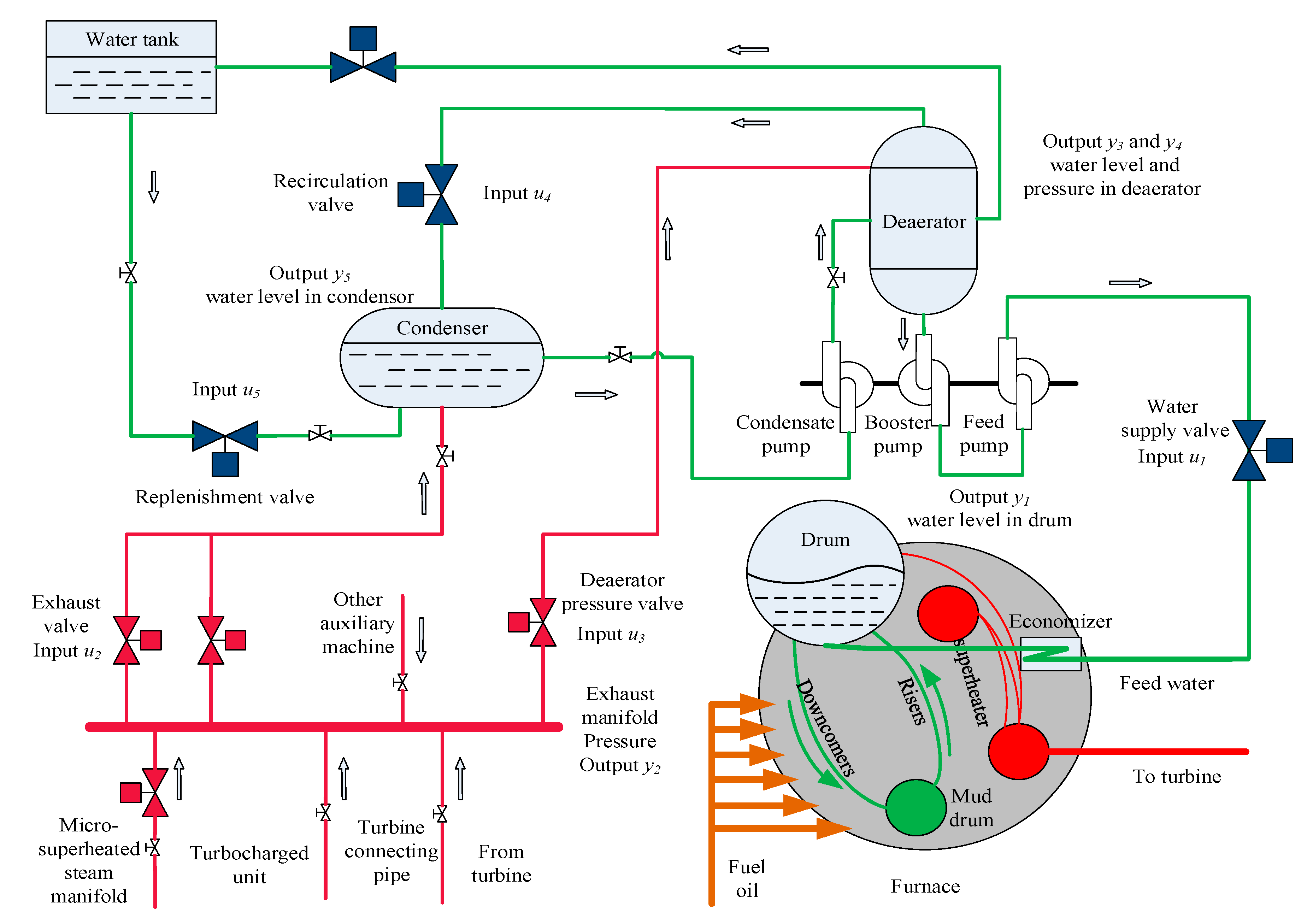
In the steam/water loop, there are mainly five loops, as briefly introduced in Figure 1: (i) drum water level control loop, (ii) deaerator water level control loop, (iii) deaerator pressure control loop, (iv) condenser water level control loop, and (v) exhaust manifold pressure control loop.

There are two main loops, one for steam indicated by red line, and another for water indicated by the green line. The system works as follows. Firstly, the water from the water tank goes to the condenser. Secondly, the water will be deoxygenated in the deaerator and be pumped to boiler. Due to a higher density of feed water, it goes into the mud drum. After being heated in the risers, the feed water turns into a mixture of steam and water. Thirdly, steam gets separated from the mixture and heated in the superheater. Finally, the steam with a certain pressure and temperature services the steam turbine. The used steam will be sent back to exhaust manifold and most of the steam gets condensed in the condenser, while the remainder services the deaerator for deoxygenation.

The references of these models for each equipment are described as follows. The model of the boiler comes from [20]; the model of exhaust manifold is approximated as a second-order model according to [21]; the models of the deaerator and condenser are obtained according to [22]. Through linearization around the operating point, the overall model shown in Equation (1) is obtained. The input vector u = [u₁,u₂,u₃,u₄,u₅] contains the positions of the valves that control the flow rates of feedwater to the drum (u₁), exhaust steam from the exhaust manifold (u₂), exhaust steam to the deaerator (u₃), water from the deaerator (u₄) and water to the condenser (u₅), respectively. The output vector y = [y₁,y₂,y₃,y₄,y₅] contains the values of the water level in drum (y₁), pressure in exhaust manifold (y₂), water level (y₃) and pressure (y₄) in the deaerator, and water level of the condenser (y₅), respectively.

Table 1. Parameters used in steam/water loop.

Output Variables	Operating Points	Range	Units
Drum water level	1.79	1.39–2.19	m
Exhaust manifold pressure	100.03	87.03–133.8	MPa
Deaerator pressure	30	24.9–43.86	KPa
Deaerator water level	0.7	0.489–0.882	m
Condenser water level	0.5	0.32–0.63	m

includes the ranges and operating points of the output variables.

$$\left[\begin{array}{c}{y}_1\\ y_2\\ ⋮\\ y_5\end{array}\right]=\left[\begin{array}{cccc}{G}_{11}& G_{12}& \cdots & G_{15}\\ G_{21}& G_{22}& \cdots & G_{25}\\ ⋮& ⋮& \ddots & ⋮\\ G_{51}& G_{52}& \cdots & G_{55}\end{array}\right]\left[\begin{array}{c}{u}_1\\ u_2\\ ⋮\\ u_5\end{array}\right]$$

(1)

where $G_{11}=\frac{0.0000987}{(s+0.1131)(s+0.0085+0.032j)(s+0.0085-0.032j)}$, $G_{22}=\frac{0.7254}{(s+1.2497)(s+0.0223)}$, $G_{23}=\frac{-0.5}{(s+1.9747)(s+0.0253)}$, $G_{33}=\frac{0.0132}{(s+0.0265+0.0244j)(s+0.0265-0.0244j)}$, $G_{34}=\frac{-0.009}{(s+0.0997)(s+0.0411)}$, $G_{41}=\frac{-0.0008}{(s+0.012+0.126j)(s+0.012-0.126j)}$, $G_{44}=\frac{0.0005152}{(s+0.012+0.038j)(s+0.012-0.038j)}$, $G_{54}=\frac{-0.00015}{(s+0.0175+0.0179j)(s+0.0175-0.0179j)}$, $G_{55}=\frac{0.00147}{(s+0.025+0.0654j)(s+0.025-0.0654j)}$, and other transfer functions $G_{12}=G_{13}=\mathrm{\dots }=G_{53}=0$.

The rates and amplitudes of the five inputs are constrained to:

$$\{\begin{array}{ll}-0.007\le \frac{d{u}_1}{dt}\le 0.007 & 0\le u_1\le 1\\ -0.01\le \frac{d{u}_2}{dt}\le 0.01& 0\le u_2\le 1\\ -0.01\le \frac{d{u}_3}{dt}\le 0.01& 0\le u_3\le 1\\ -0.007\le \frac{d{u}_4}{dt}\le 0.007& 0\le u_4\le 1\\ -0.007\le \frac{d{u}_5}{dt}\le 0.007& 0\le u_5\le 1\end{array}$$

(2)

The inputs units are normalized percentage values of the valve opening (i.e., 0 represents a fully closed valve, and 1 is completely opened). Additionally, the input rates are measured in percentage per second.

3. Model Predictive Control with Optimized Control Horizon

3.1. Brief Introduction to Extended Prediction Self-Adaptive Control (EPSAC)

The following is a short summary of EPSAC and more details can be found in [23]. Consider a linear system described below:

$$y(t)=x(t)+n(t)$$

(3)

where $y(t)$ indicates the measured output of system; $x(t)$ is the output of model and $n(t)$ is the model/process disturbance. The output of the model $x(t)$ depends on the past outputs and inputs, and can be expressed generically as:

$$x(t)=f[x(t-1),x(t-2),\dots ,u(t-1),u(t-2),\dots ]$$

(4)

In EPSAC, the future input consists of two parts:

$$u(t+k|t)=u_{base}(t+k|t)+\delta u(t+k|t)$$

(5)

where $u_{base}(t+k|t)$ indicates basic future control scenario and $\delta u(t+k|t)$ indicates the optimizing future control actions. Then following results will be obtained by applying Equation (5) as the control effort.

$$y(t+k|t)=y_{base}(t+k|t)+y_{opt}(t+k|t)$$

(6)

where $y_{base}(t+k|t)$ is the effect of base future control and $y_{opt}(t+k|t)$ is the effect of optimizing future control actions $\delta u(t|t)$, …, $\delta u(t+N_c-1|t)$. The part of $y_{opt}(t+k|t)$ can be expressed as a discrete time convolution as follows:

$$y_{opt}(t+k|t)=h_k\delta u(t|t)+h_{k-1}\delta u(t+1|t)+\dots +g_{k-N_c+1}\delta u(t+N_c-1|t)$$

(7)

where h₁, … h_Np are impulse response coefficients; g₁, … g_Np are the step response coefficients; N_c, N_p are control horizon and prediction horizon, respectively. Thus the following formulation can be obtained:

$$\mathbf{Y}=\overline{\mathbf{Y}}+\mathbf{G}·\mathbf{U}$$

(8)

with, $\mathbf{Y}={[y(t+N_1|t)\dots y(t+N_p|t)]}^T$, $\mathbf{U}={[\delta u(t|t)\dots \delta u(t+N_c-1|t)]}^T$, $\overline{\mathbf{Y}}={[y_{base}(t+N_1|t)\dots y_{base}(t+N_P|t)]}^T$ and

$$\mathbf{G}=\left[\begin{array}{cccc}{h}_{N_1}& h_{N_1-1}& \dots & g_{N_1-N_c+1}\\ h_{N_1+1}& h_{N_1}& \dots & \dots \\ \dots & \dots & \dots & \dots \\ h_{N_P}& h_{N_P-1}& \dots & g_{N_P-N_c+1}\end{array}\right]$$

(9)

where N₁ indicates the time-delay in the system.

The disturbance term $n(t)$ is defined as a filtered white noise signal [19]. When there is no information concerning the noise, the disturbance model used in Equation (3) can be chosen as an integrator, to ensure zero steady-state error in the reference tracking experiment:

$$n(t)=\frac{1}{1-q^{-1}}e(\mathrm{t})$$

(10)

where e(t) denotes the white noise; $q^{-1}$ is the backward shift operator.

In order to apply EPSAC for a MIMO (multiple-input and multiple-output) system, the individual error of each output is minimized separately. The cost function for the steam/water system with five sub-loops is as follows:

$$J_i=\sum _{k=N_1}^{N_P}{[r_i(t+k|t)-y_i(t+k|t)]}^2\hspace{1em}(i=1,2,\dots ,5)$$

(11)

By defining G_ik as the influence from kth input to ith output, Equation (11) can be rewritten as:

$${({\mathbf{R}}_i-{\mathbf{Y}}_i)}^T({\mathbf{R}}_i-{\mathbf{Y}}_i)=({\mathbf{R}}_i-{\overline{\mathbf{Y}}}_i-\sum _{k=1}^5{\mathbf{G}}_{ik}{\mathbf{U}}_k{)}^T({\mathbf{R}}_i-{\overline{\mathbf{Y}}}_i-\sum _{k=1}^5{\mathbf{G}}_{ik}{\mathbf{U}}_k)$$

(12)

with R_i denoting the reference for loop i, and Y_i denotes the predicted output for loop i.

Taking constraints from inputs and outputs into account, the process to find the minimum cost function becomes an optimization problem which is called quadratic programming.

$$\begin{array}{l}\underset{{\mathbf{U}}_i}{\mathbf{min}}{\mathbf{J}}_i({\mathbf{U}}_i(={{\mathbf{U}}_i}^T{\mathbf{H}}_i{\mathbf{U}}_i+2{{\mathbf{f}}_i}^T{\mathbf{U}}_i+c_i \mathrm{subject} \mathrm{to} \mathbf{A}\mathbf{U}\le \mathbf{b}\\ \mathrm{with}\{\begin{array}{l} {\mathbf{H}}_i={\mathbf{G}}_{ii}^T{\mathbf{G}}_{ii}\hspace{1em}\hspace{1em}{\mathbf{f}}_i=-{\mathbf{G}}_{ii}^T({\mathbf{R}}_i-{\overline{\mathbf{Y}}}_i-{\displaystyle \sum _{k=1}^5{\mathbf{G}}_{ik}{\mathbf{U}}_k})\\ c_i=({\mathbf{R}}_i-{\overline{\mathbf{Y}}}_i-{\displaystyle \sum _{k=1}^5{\mathbf{G}}_{ik}{\mathbf{U}}_k}{)}^T({\mathbf{R}}_i-{\overline{\mathbf{Y}}}_i-{\displaystyle \sum _{k=1}^5{\mathbf{G}}_{ik}{\mathbf{U}}_k})\end{array}\end{array}$$

(13)

where A is a matrix; b is a vector according to the constraints and U_i is the input for sub loop i. By solving the quadratic problem, the optimal U = [U₁ U₂ U₃ U₄ U₅] can be obtained.

3.2. Ripple-Free Model Predictive Control (MPC)

Since MPC uses a discrete-time model, it is easy to get ripples in the system output when controlling a continuous system with periodic control effort during the sampling time. According to the simulation results of the steam/water loop in large-scale ships, there always exists ripple when applying a control horizon $N_c\ge 2$. To remove the ripple in the control effort, an alternative cost function which also penalizes the control effort imposed in the EPSAC strategy [15], obtaining:

$$J_i=J_i^e+\frac{\lambda }{1-\lambda }{J}_i^u$$

(14)

where $\lambda \in [0; 1)$ is a weighting parameter, and,

$$J_i^e=\sum _{k=1}^{N_p}k{e}_i{(t+k|t)}^2,\hspace{1em}{J}_i^u=\sum _{k=1}^{N_c}{\left(u_i(t+k|t)-u_i(t+k- 1|t)\right)}^2$$

(15)

are the cumulative sum that penalizes the predicted tracking error e_i(t + k|t) over the prediction horizon, and the cumulative term which corrects the deviations in postulated control effort u_i(t + k|t) over the control horizon, for each loop i, respectively.

In order to minimize the $J_i^e$ in Equation (15), the tracking error must converge to zero rapidly. However, the $J_i^u$ term has a negative impact on the tracking error. By choosing an appropriate value for $\lambda$, a good trade-off between the closed-loop performance and the control effort can be made.

3.3. Optimized Control Horizon

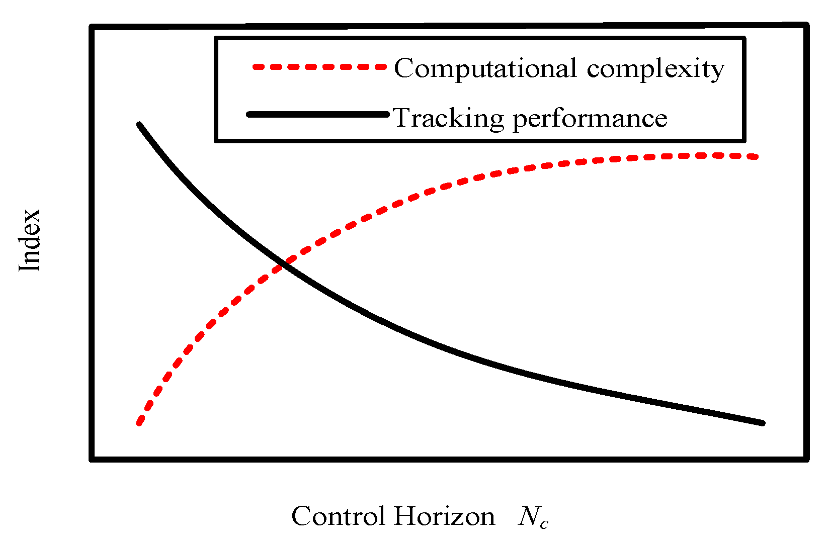
To our knowledge, the longer control horizon values can result in better performance, albeit the computational complexity will also increase, which makes it more difficult to realize online optimization. The relationship between performance, computational complexity and control horizon can be described by Figure 2.

According to Figure 2, it is possible to find a good trade-off between the tracking performance and computational complexity. In this paper, the problem is explicitly treated as an optimization problem, and the following index is applied to obtain the point of compromise for the five loops [24]:

$$\begin{array}{l}{I}_i=T_i+{\eta }_i{E}_i\hspace{1em}\hspace{1em}(i=1,2,\dots ,5)\\ T_i={\displaystyle \sum _{k=1}^{N_S}{t}_{is}(k)}\hspace{1em}{E}_i={\displaystyle \sum _{k=0}^{N_S}\left|r_i(k)-y_i(k)\right|/r_i}(k)\end{array}$$

(16)

where T_i is the total simulation computation time, with t_is the length of time required to perform the optimization at each sampling time and N_s the number of total simulation samples; E_i is the integrated absolute normalized tracking error; ${\eta }_i$ denotes the weighting factor.

In order to obtain the optimal control horizon N_c for loop i, experiments are required to be conducted with different control horizons. After minimizing the index I_i, the optimal control horizon can be obtained. The value of $\eta$ should be chosen according to the dynamic of the system. For example, the dynamic of the system is slow in the steam/water loop, hence a large value of $\eta$ should be chosen to focus more on the error than the computation time.

4. Simulation Results and Analysis

In this section, the proposed EPSAC method is applied to the steam/water loop. Firstly, the performance is shown after applying the cost function focus on penalizing the control effort by tracking several step set points in different loops. Secondly, different control horizon sets are imposed in the ripple-free EPSAC to verify their effect, and the optimal control horizon set is obtained by minimizing the index in Equation (16).

4.1 Ripple-Free Validation

According to our previous work, the parameter configuration for the EPSAC method is shown in

Table 2. Parameters applied in Extended Prediction Self-Adaptive Control (EPSAC) controller.

Controllers	Nc	Ts	Np	λ	N1	Ns
EPSAC	10	5 s	Np1 = 20; Np2 = 15; Np3 = 15; Np4 = 20; Np5 = 20	0	1	300
Ripple-free EPSAC				0.3

, where the T_s is the sampling time; N_p1, N_p2, …, N_p5 are prediction horizons of the five loops, respectively. (The prediction horizons were selected taking into account the specific transient dynamic for each loop). The step set points are provided in

Table 3. Step set points changes in the experiments.

Time (s)	2–300	300–600	600–900	900–1200	1200–1500
Drum Water Level (m)	2	2	2	2	2
Exhaust Manifold Pressure (MPa)	100.03	116	116	116	116
Deaerator Pressure (KPa)	30	30	35	35	35
Deaerator Water Level (m)	0.7	0.7	0.7	0.8	0.8
Condenser Water Level (m)	0.5	0.5	0.5	0.5	0.6

. In the experiments, the initial condition was set at the operating point of the steam/water loop.

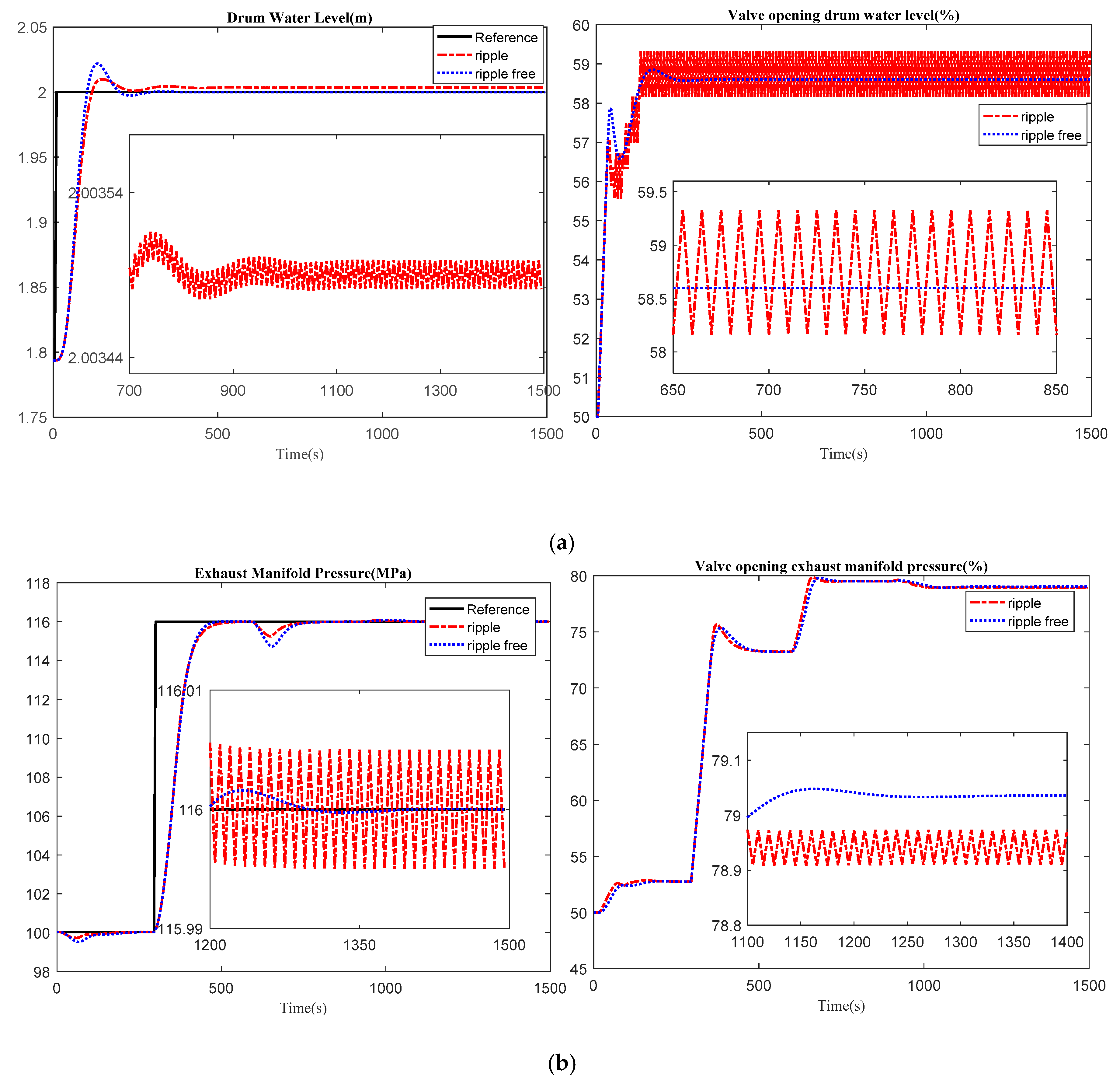
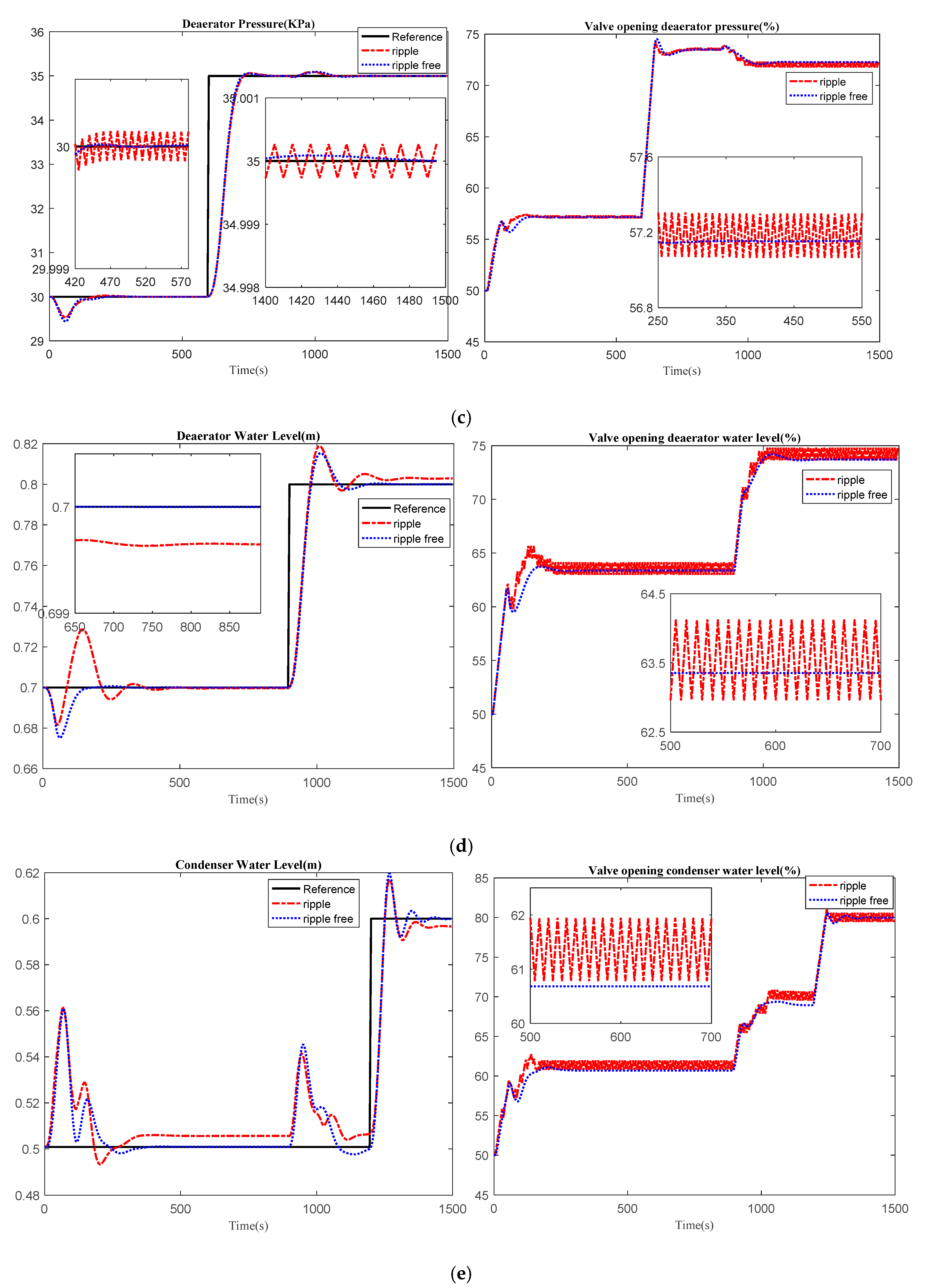
The simulation results are shown in Figure 3, including the system outputs and the corresponding control efforts. Note that the EPSAC performs better, with the cost function given in Section 3.2 that also penalizes the control effort variations, thus eliminating the severe ripples on each loop input. Also, it is noteworthy to mention that the output steady state error from loops 1, 4 and 5 is removed.

When only the tracking error is penalized in the cost function, there are ripples with N_c ≥ 2, which means that the controller is allowed to give at least two different control values, to ensure that the predicted output reaches the imposed reference, within the prediction window. In order to minimize the cost function, the first value of control effort will be optimized as large as possible under the constraint of the system. Hence, the inputs of the system are aggressive which results in the ripples. The amplitude of the ripples is influenced by the control horizon and the sampling time. By choosing an appropriate λ value in Equation (14), the ripples can be effectively removed. It is worth mentioning that when the control horizon is N_c = 1, there are no ripples.

In the ship’s steam/water loop, the condenser and the deaerator have smaller capacity when compared with the boiler. Therefore, as seen in Figure 3, there are large overshoot values at the condenser water level and the deaerator water level when the setpoint is changing for the drum water level. The steady errors exhibited in loops 1, 4 and 5 as shown in Figure 3, are caused by the intrinsic coupling between the respective loops. The input u₁ has a large influence on the deaerator water level y₄, which is controlled by u₄. However, input u₄ also modifies the condenser water level y₅. On the other hand, the inputs for each loop are calculated according to the cost function shown in Equation (12), where the past sample time input values for the coupling variables are used.

4.2. Influence of Different Control Horizon Sets

This section summarizes the results for the five loops with different control horizon values. The simulation study cases are described as follows:

• Case 1: N_c1,…,N_c5 = 1 sample;
• Case 2: N_c1,…,N_c5 = 2 samples;
• Case 3: N_c1,…,N_c5 = 5 samples;
• Case 4: N_c1,…,N_c5 = 10 samples.

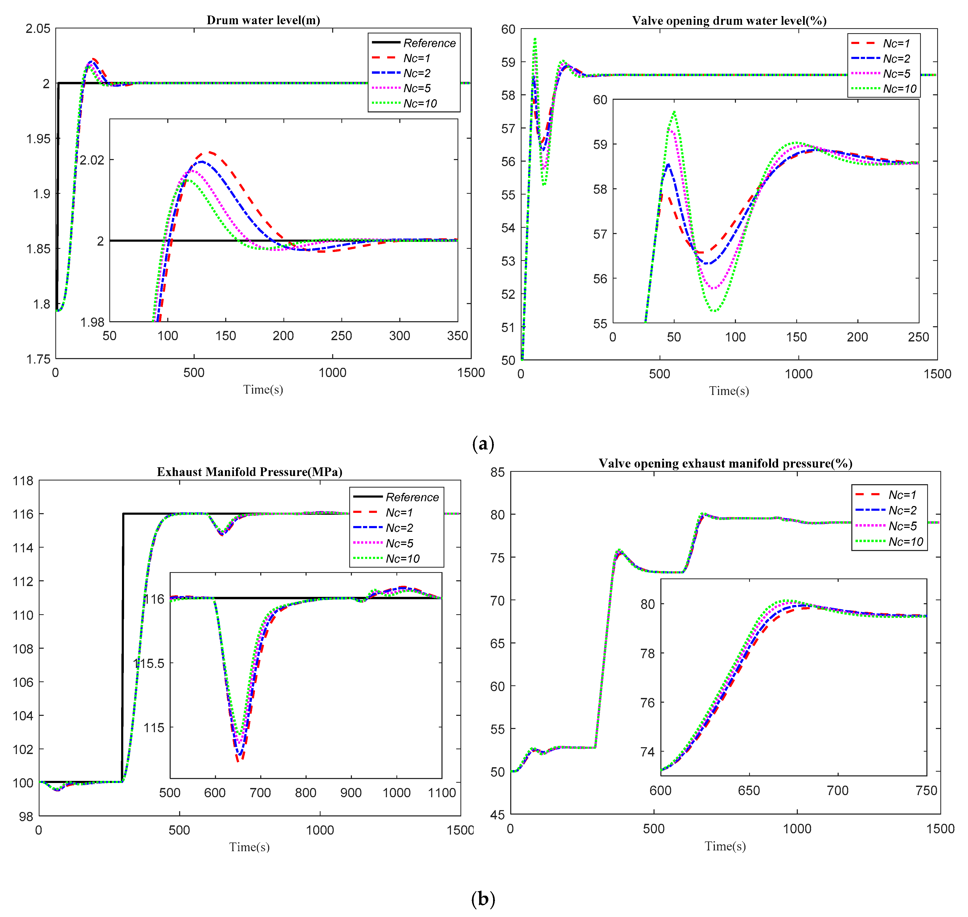
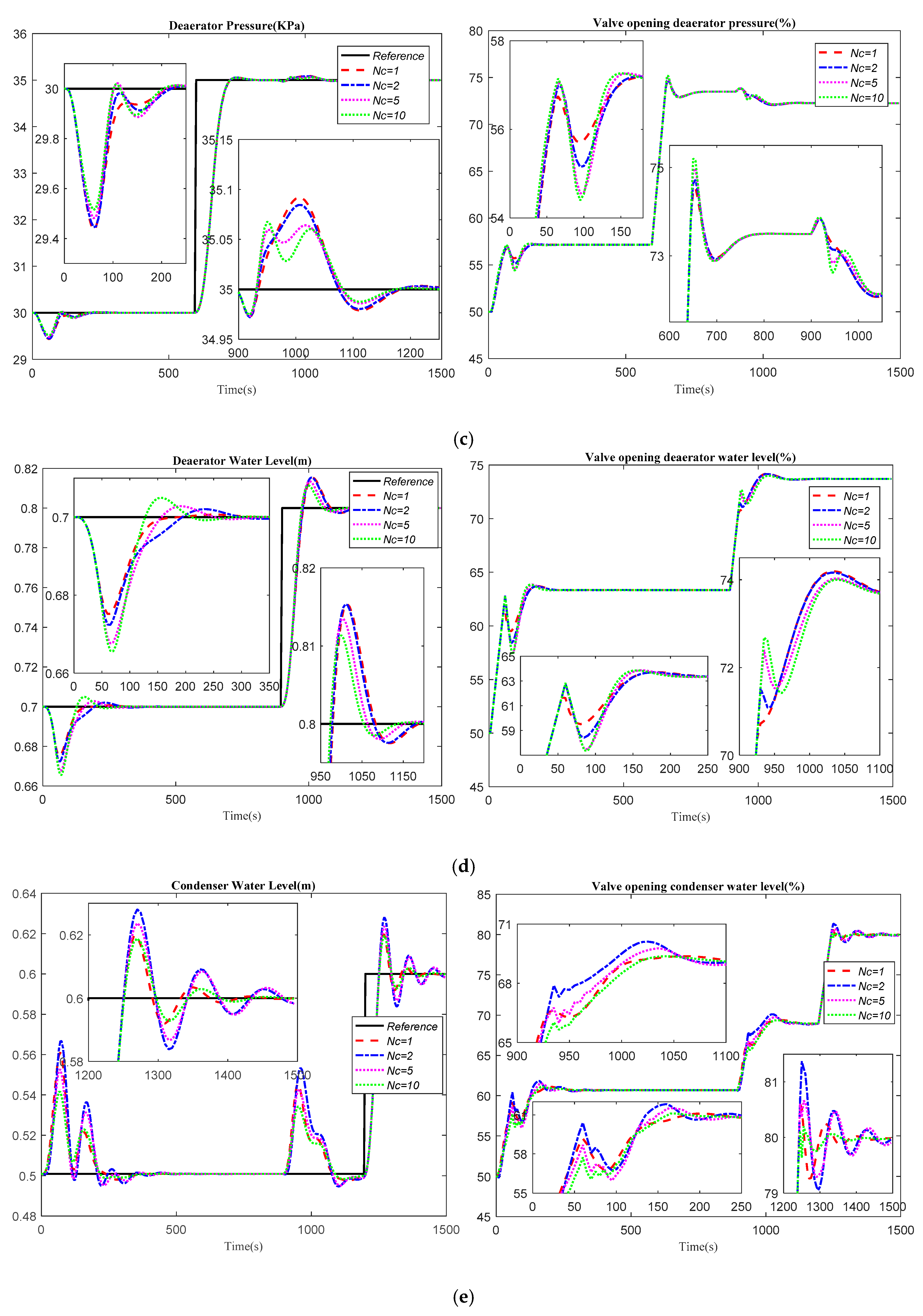
The responses of the steam/water loop with different control horizon values, are shown in Figure 4 (left-hand side), whereas the corresponding control efforts are given in Figure 4 (right-hand side). From the simulation results, one can remark that increasing the control horizon value in the proposed ripple-free EPSAC leads to better tracking performance, with a smaller overshoot and settling-time response, but with a higher control effort.

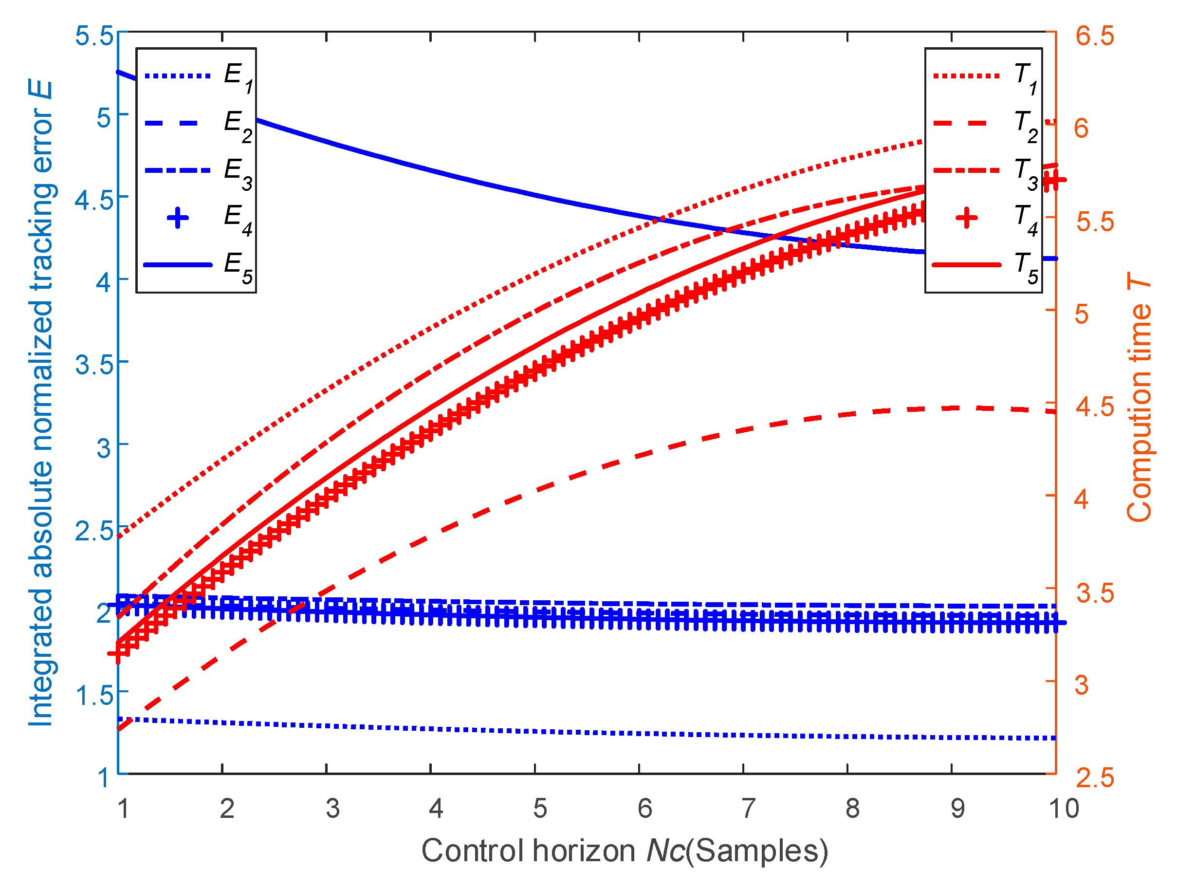
The performance of the proposed ripple-free EPSAC algorithm was also analyzed in terms of the integrated absolute normalized tracking error (E_i) and computation time (T_i) defined in Section 3.3, in index (15). The numerical values are listed in

Table 4. Normalized tracking error with different control horizon sets.

	Loop 1	Loop 2	Loop 3	Loop 4	Loop 5
Nc = 1	1.342	2.039	2.08	1.933	4.603
Nc = 2	1.294	2.007	2.063	2.04	5.595
Nc = 5	1.242	1.976	2.038	1.999	5.012
Nc = 10	1.215	1.957	2.015	1.919	4.147

and

Table 5. Computing time in seconds with different control horizon sets.

	Loop 1	Loop 2	Loop 3	Loop 4	Loop 5
Nc = 1	3.384	2.687	3.182	2.584	2.79
Nc = 2	4.778	3.217	4.083	4.432	4.297
Nc = 5	6.058	4.456	5.716	5.757	5.822
Nc = 10	5.959	4.393	5.195	5.332	5.455

respectively, and their relationship is graphically depicted in Figure 5 (for different control horizon values).

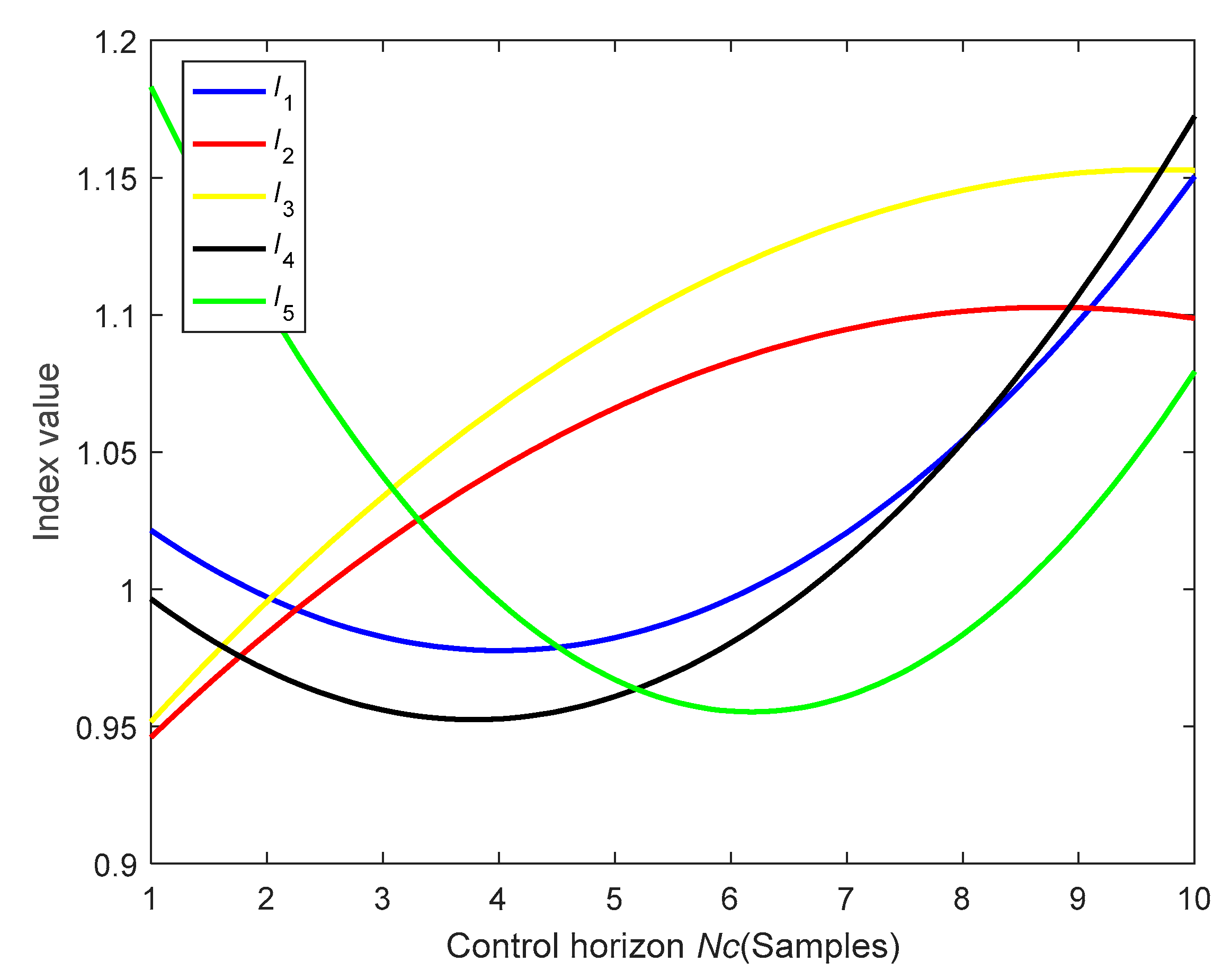
Next, the information from Table 4 and Table 5 is combined, and the index (16) is calculated, with ${\eta }_i$ = 0.76, for each loop i (i = 1,2,…,5). Note that this value compromises the computational complexity (i.e., the required computation time) in favor of a better tracking error. Given the graphical results plotted in Figure 6 and their significance, the optimal N_c set is selected as N_c1 = 4, N_c2 = 1, N_c3 = 1, N_c4 = 4, N_c5 = 6 samples, which gives a good trade-off between the two components from index (15).

5. Conclusions

In this paper, the effect of control horizon is studied for an EPSAC model predictive control framework, and the results are validated on a complex steam/water loop process example. Since a larger control horizon improves the performance of the system at the price of a higher computational complexity and control effort, a trade-off is required. By minimizing an objective function defined as a combination between the system error and computational time, the best control horizon set of values is obtained. According to the simulation results, when applying different control horizon sets ($N_c\ge 2$) in the steam/water loop, there are always ripples in the output of the system. Hence, a cost function in terms of tracking error and deviations in the control effort was imposed in EPSAC. The simulation results show the effectiveness of the alternative cost function from EPSAC.

References

- Sun, L.; Hua, Q.; Li, D.; Pan, L.; Xue, Y.; Lee, K.Y. Direct energy balance based active disturbance rejection control for coal-fired power plant. ISA Trans. 2017, 70, 486–493. [Google Scholar] [CrossRef] [PubMed]
- Zhao, S.; Ionescu, C.M.; De Keyser, R.; Liu, S. A Robust PID Autotuning Method for Steam/Water Loop in Large Scale Ships. In Proceedings of the 3rd IFAC Conference in Advances in Proportional-Integral-Derivative Control, Ghent, Belgium, 9–11 May 2018; pp. 462–467. [Google Scholar]
- Hosseinzadeh, M.; Yazdanpanah, M.J. Robust adaptive passivity-based control of open-loop unstable affine non-linear systems subject to actuator saturation. IET Control Theory Appl. 2017, 11, 2731–2742. [Google Scholar] [CrossRef]
- Wang, W.L.A.; Mukai, H. Stability of linear time-invariant open-loop unstable systems with input saturation. Asian J. Control 2004, 6, 496–506. [Google Scholar] [CrossRef]
- Scarciotti, G.; Astolfi, A. Approximate finite-horizon optimal control for input-affine nonlinear systems with input constraints. J. Control Decis. 2014, 1, 149–165. [Google Scholar] [CrossRef]
- Li, Y.; Li, T.; Tong, S. Adaptive fuzzy modular backstepping output feedback control of uncertain nonlinear systems in the presence of input saturation. Int. J. Mach. Learn. Cybern. 2013, 4, 527–536. [Google Scholar] [CrossRef]
- Maxim, A.; Copot, D.; De Keyser, R.; Ionescu, C.M. An industrially relevant formulation of a distributed model predictive control algorithm based on minimal process information. J. Process Control 2018, 68, 240–253. [Google Scholar] [CrossRef]
- Fu, D.; Zhang, H.; Yu, Y.; Ionescu, C.M.; Aghezzaf, E.; De Keyser, R. A Distributed Model Predictive Control Strategy for Bullwhip Reducing Inventory Management Policy. IEEE Trans. Ind. Inf. 2018, in press. [Google Scholar] [CrossRef]
- Liu, X.; Cui, J. Economic model predictive control of boiler-turbine system. J. Process Control 2018, 66, 59–67. [Google Scholar] [CrossRef]
- Wu, X.; Shen, J.; Li, Y.; Lee, K.Y. Fuzzy modeling and stable model predictive tracking control of large-scale power plants. J. Process Control 2014, 24, 1609–1626. [Google Scholar] [CrossRef]
- Liu, X.J.; Chan, C.W. Neuro-fuzzy generalized predictive control of boiler steam temperature. IEEE Trans. Energy Convers. 2006, 21, 900–908. [Google Scholar] [CrossRef]
- Liu, X.; Guan, P.; Chan, C.W. Nonlinear multivariable power plant coordinate control by constrained predictive scheme. IEEE Trans. Control Syst. Technol. 2010, 18, 1116–1125. [Google Scholar] [CrossRef]
- Liu, X.; Kong, X. Nonlinear fuzzy model predictive iterative learning control for drum-type boiler–turbine system. J. Process Control 2013, 23, 1023–1040. [Google Scholar] [CrossRef]
- Havlena, V.; Findejs, J. Application of model predictive control to advanced combustion control. Control Eng. Pract. 2005, 13, 671–680. [Google Scholar] [CrossRef]
- Zhao, S.; Cajo, R.; De Keyser, R.; Ionescu, C.M. Nonlinear predictive control applied to steam/water loop in large scale ships. In Proceedings of the 12th IFAC Symposium on Dynamics and Control of Process Systems, including Biosystems (under review).
- Rossiter, J.A. Model-Based Predictive Control: A Practical Approach; CRC Press: Boca Raton, FL, USA, 2003; pp. 85–102. [Google Scholar]
- Ohtsuka, T. A continuation/GMRES method for fast computation of nonlinear receding horizon control. Automatica 2004, 40, 563–574. [Google Scholar] [CrossRef]
- Cortés, P.; Kazmierkowski, M.P.; Kennel, R.M.; Quevedo, D.E.; Rodríguez, J. Predictive control in power electronics and drives. IEEE Trans. Ind. Electron. 2008, 55, 4312–4324. [Google Scholar]
- De Keyser, R. Model based predictive control for linear systems. In Control Systems, Robotics and Automation-Volume XI Advanced Control Systems-V; Unbehauen, H., Ed.; UNESCO: Oxford, UK, 2003; pp. 24–58. [Google Scholar]
- Åström, K.J.; Bell, R.D. Drum-boiler dynamics. Automatica 2000, 36, 363–378. [Google Scholar]
- Wang, P.; Liu, M.; Ge, X. Study of the improvement of the exhaust steam maniline pressure control system of a steam-driven power plant. J. Eng. Therm. Energy Power 2014, 29, 65–70. [Google Scholar]
- Wang, P.; Meng, H.; Dong, P.; Dai, R. Decoupling control based on pid neural network for deaerator and condenser water level control system. In Proceedings of the 34th Chinese Control Conference (CCC), Hangzhou, China, 28–30 July 2015; pp. 3441–3446. [Google Scholar]
- De Keyser, R.; Ionescu, C.M. The disturbance model in model based predictive control. In Proceedings of the IEEE Conference on Control Applications (CCA 2003), Istanbul, Turkey, 25–25 June 2003; pp. 446–451. [Google Scholar]
- Ribeiro, C.C.; Rosseti, I.; Souza, R.C. Effective probabilistic stopping rules for randomized metaheuristics: GRASP implementations. In Learning and Intelligent Optimization; Springer: Berlin, Germany, 2011; Volume 6683, pp. 146–160. [Google Scholar]
Figure 1.
Scheme of complete steam/water loop investigated in this paper.
Figure 2.
The relationship between tracking performance, computational complexity and control horizon.
Figure 3.
Responses of the steam/water loop under the EPSAC and ripple-free EPSAC for (a) drum water level control loop, (b) deaerator water level control loop, (c) deaerator pressure control loop, (d) condenser water level control loop and (e) exhaust manifold pressure control loop (The figures on left-hand indicate the outputs, and on the right-hand indicate the inputs).
Figure 4.
Responses of the steam/water loop under the ripple-free EPSAC for different control horizons for (a) drum water level control loop, (b) deaerator water level control loop, (c) deaerator pressure control loop, (d) condenser water level control loop and (e) exhaust manifold pressure control loop (The figures on left-hand indicate the outputs, and on the right-hand indicate the inputs).
Figure 5.
Computation time Ti (blue line) and integrated absolute normalized tracking error Ei (red line) in the five loops i (i = 1,2,…,5) for different control horizon values.
Figure 6.
Optimization index for different control horizon values.