Eulerian Multiphase Simulation of the Particle Dynamics in a Fluidized Bed Opposed Gas Jet Mill


1
Institute of Chemistry, Federal University of Goiás—UFG, Goiânia-GO 74690-900, Brazil
2
Institute of Particle Technology, Friedrich-Alexander University, 91058 Erlangen, Germany
*
Author to whom correspondence should be addressed.
Processes 2020, 8(12), 1621; https://doi.org/10.3390/pr8121621
Submission received: 26 October 2020
/
Revised: 25 November 2020
/
Accepted: 3 December 2020
/
Published: 9 December 2020
(This article belongs to the Special Issue Recent Advances in Fluidized Bed Hydrodynamics and Transport Phenomena)
Abstract
:The compressible and turbulent gas–solid multiphase flow inside a fluidized bed opposed jet mill was systematically investigated through numerical simulations using the Euler–Euler approach along with the kinetic theory of granular flow and frictional models. The solid holdup and nozzle inlet air velocity effects on the gas–solid dynamics were assessed through a detailed analysis of the time-averaged volume fraction, the time-averaged velocity, the time-averaged streamlines, and the time-averaged vector field distributions of both phases. The simulated results were compared with the experimental observations available in the literature. The numerical simulations contributed to a better understanding of the particle–flow dynamics in a fluidized bed opposed gas jet mill which are of fundamental importance for the milling process performance.
1. Introduction
Comminution is a major size reduction process in solids processing. To break a particle, critical stress must be provided to the material. The number of stressing events and the magnitude of each event depends on the design of the apparatus. Comminution by stresses induced by mechanical forces is performed for instance in ball mills, hammer mills, planetary mills, oscillating mills, and fluidized bed jet mills which are in widespread use in various industries such as minerals, foods, pharmaceuticals, and ceramics. Concerning achieving a desired size and shape distribution of the product, comminution poses many challenges, stemming from the material characteristics, for example, initial size, elasticity and plasticity of the material, and process conditions [1].
A fluidized bed opposed jet mill is commonly comprised of three different regions: the grinding region, where the pressurized air is injected through the nozzles; the transport region, where the particles are pushed upward by the nozzles’ gas jets in the grinding region; and the classifying region, at the top of the equipment which consists of one or more classifier wheels rotating at a certain velocity depending on the desired particle cut size. The coarse fraction is recycled to the grinding region, whereas the fine ones are discharged as product. This equipment, which is used for instance in the production of dry abrasion- and contamination-free pharmaceutical powders, involve complex particle–particle and particle–fluid interactions due to the presence of a highly expanded and turbulent gas jet which are still poorly understood [2].
Thus far, a limited number of works has focused on the investigation of the influence of operating parameters, such as solid holdup, inlet air pressure, and jet nozzle number and configuration, on the particle dynamics behavior in a fluidized bed opposed jet mill. Their design and prediction of performance are until now, largely empirical [1,2,3,4,5,6]. Especially the dynamic interaction of the fluid with the solid phase, for instance at the focal point of the jets (grinding region), is poorly understood—in part because of the difficulties in measurement of the process conditions at this point.
Numerical simulation, based on the governing principles of mass and momentum transfer, can be utilized to fundamentally investigate the fluid–solids interaction inside different equipment, connect material properties and process conditions to measured results, thus sequentially removing empiricism towards predictive design and operation. For multiphase modeling of granular flow, i.e., the fluid–solid interaction, the Euler–Euler, and the Euler–Lagrange approaches are commonly used [7,8].
In the Euler–Euler approach, all phases are treated as interpenetrating continua, i.e., the solid particles are treated as a continuous phase with effective parameters. The corresponding differential equations of momentum, mass, and energy are solved on a Eulerian frame of reference. This approach is utilized in many computational fluid dynamics techniques (CFD) [9].
In the Euler–Lagrange approach, the fluid phase is treated as continuum while each particle in the disperse phase is tracked solving Newton’s second law, thus allowing resolving particle–particle, particle–boundary, and particle–flow interaction. The Euler–Lagrange approach is implemented by coupling CFD techniques, for fluid phases, and, e.g., the Discrete Element Method (DEM), for solid phases [10].
A major drawback of the Euler–Lagrange approach is the substantial numerical effort required with systems comprised of large number of particles and high Re-numbers, such as those found in fluidized bed jet mills. Thus, this approach is commonly restricted to reduced scale equipment under low flow rates. On the other hand, the Euler–Euler approach has been successfully applied in the prediction of the fluid-particle dynamics in different processes [8,11,12,13].
Only very few numerical studies have been performed so far concerning the particle dynamics in fluidized bed jet mills [14,15], whereas the majority of the simulations in jet mills are restricted to spiral jet-mill systems [16,17,18,19,20]. Furthermore, experimental data of the particle–flow dynamics in a fluidized opposed gas jet mill, which are of crucial importance for the numerical model validation, are extremely scarce in the literature. Most of the experimental studies are focused on the milling process itself.
Thus, the objective of this work is a fundamental study of the particle–fluid dynamics behavior in a fluidized bed opposed jet mill. The compressible and turbulent gas–solid multiphase flow was simulated through the Euler–Euler approach along with the kinetic theory of granular flow and frictional models. The effects of solid holdup and nozzle inlet air velocity on the particle behavior were accessed. The simulation results were compared with the available experimental observations in the literature.
The structure of the contribution is as follows: First, Section 2 describes the suitable set of formulation in the Euler–Euler approach for the simulation of the turbulent and compressible solid–gas multiphase flow in a fluidized bed opposed jet mill. The fluidized bed geometry, material properties, and operating conditions are also described. Section 3 is devoted to the presentation and discussion of the numerical results based on the experimental observations reported in the literature. The paper is closed with conclusions in Section 4.
2. Materials and Methods
2.1. Fluidized Bed Opposed Jet Mill Unit and Material Properties
The fluidized bed geometry and operating conditions used in all simulations were based on the experimental works available in the literature [2,3,6].
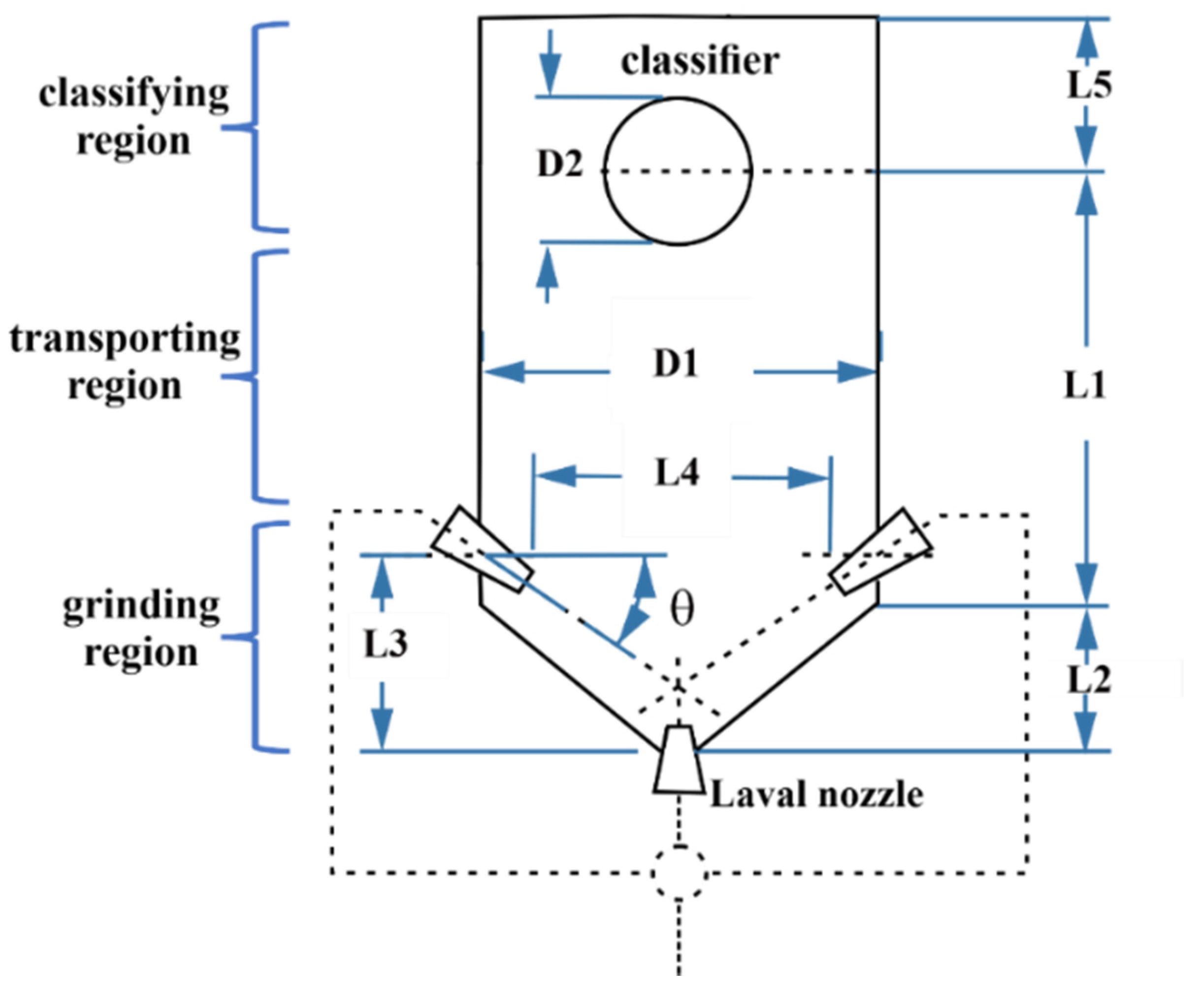
A schematic representation of the fluidized bed opposed gas jet mill (AFG 100, Hosokawa Alpine, Augsburg, Germany) and all the geometric parameters are shown in Figure 1 and Table 1, respectively.
The jet mill is composed of a classifier wheel of 0.05 m in outer diameter, placed at the upper part of the equipment (classifying region), and three Laval nozzles with an exit diameter of 2.4 mm (Dnozzle) positioned in the grinding region, one at the bottom, and two at the lateral wall of the equipment inclined at an angle of 30° and separated by a distance of 65.4 mm (Figure 1). Glass microspheres with a mean diameter of 55 μm and a density of 2500 kg/m3 [6], were used. The porosity of the packed bed was of 0.38.
2.2. Eulerian Multiphase Modeling
In the Euler–Euler approach, both gas and solid phases are treated as interpenetrating continua whose fundamental and constitutive equations are solved on a Eulerian frame of reference. To model the viscous solid stress tensor, the kinetic theory of granular flow, developed by Lun et al. [9], was applied.
Due to the high-velocity gas jets inside the fluidized bed (high Reynolds number), the effects of turbulence and compressibility on the solid-fluid flow were taken into consideration. The kf-εf turbulence model was used to estimate the fluctuations of the gas’ properties due to turbulence. To account for the gas compressibility, the state equation of the ideal gas was employed.
The main equations are summarized in the following: Equations (1) and (2) represent the mass conservation, while Equations (3) and (4) represent the momentum conservation for the gas and solid phases (compressible flow), respectively:
where , ,,, , , , , , ,
, and are, respectively, the gas and solid velocity vectors, the gas and solid volume fractions, the gas and solid densities, the gas and solid pressures, the gas and solid viscous stress tensors, the gravity acceleration vector, and the solid–gas momentum exchange coefficient.
The constitutive equations for the Euler–Euler approach closure are summarized in Table 2.
The kinetic, and collisional granular viscosity and pressure are functions of the granular temperature (ψs), which measures the particle velocity fluctuation in analogy with the thermodynamic temperature [9]. The transport equation for granular temperature is given as follows:
where , , and are the conductivity of the granular temperature (Equation (16)), the kinetic energy dissipation due to inelastic collisions (Equation (17)), and the kinetic energy dissipation due to fluid friction (Equation (18)), respectively.
Frictional effects take place when the particle concentration reaches a critical value (αsc). In this work, Schaeffer’s model [21] (Equation (10)), and Johnson and Jackson’s model [22] (Equation (13)) were used to calculate the frictional viscosity and the frictional pressure, respectively. The following parameters were used for the Eulerian granular models shown in Table 2: αsc = 0.5, = 0.62, = 0.94, and = 28.5.
To calculate the effective fluid viscosity () for the fluid viscous stress tensor (Equation (5)), which is a function of the fluid dynamic viscosity () and the turbulent fluid viscosity (), the kf-εf turbulent model was used. In this model, the turbulent viscosity is represented by , whose kf and εf values are calculated as follows:
where kf and εf are, respectively, the turbulent kinetic energy and the turbulent kinetic energy dissipation rate, and are the dispersed phase turbulence influences on the continuous phase [24,25], and G is the turbulent kinetic energy production rate. The empirical constants are: = 0.09, = 1.44, = 1.92, = 1.0, and = 1.3 [26].
To take into consideration viscous dissipation in the fluid at high fluid velocity in the internal energy and flow compressibility, the energy equation was also solved (Equation (25)). The subscript index “i” stands for either solid or fluid phases.
where , k, , and are the enthalpy, the kinetic energy, the effective thermal diffusivity, and the convective heat transfer between the solid and fluid phases, respectively. The convective heat transfer coefficient is represented by , where is the thermal fluid conductivity, ds is the particle diameter, and Nu is the Nusselt number calculated herein by Ranz and Marshall’s correlation [27].
Finally, to model the momentum transfer between fluid and solid phase, the Gidaspow drag model [23] was used. Gidaspow [23] proposed a combination of the Wen and Yu drag model [28] (Equation (19)) for dilute systems () and the Ergun model [29] (Equation (20)) for dense systems (). This model has been successfully applied for the particle–fluid dynamics studies in different systems [11,30,31].
An interesting comparison between different drag models can be found in Upadhyay et al. [32].
2.3. Numerical and Boundary Conditions
For all transient, compressible, and turbulent simulations, the open-source CFD code OpenFOAM®, version 5.x (twoPhaseEulerFoam solver), and the open-source multi-platform data analysis and visualization software ParaView®, version 5.8.1, were used.
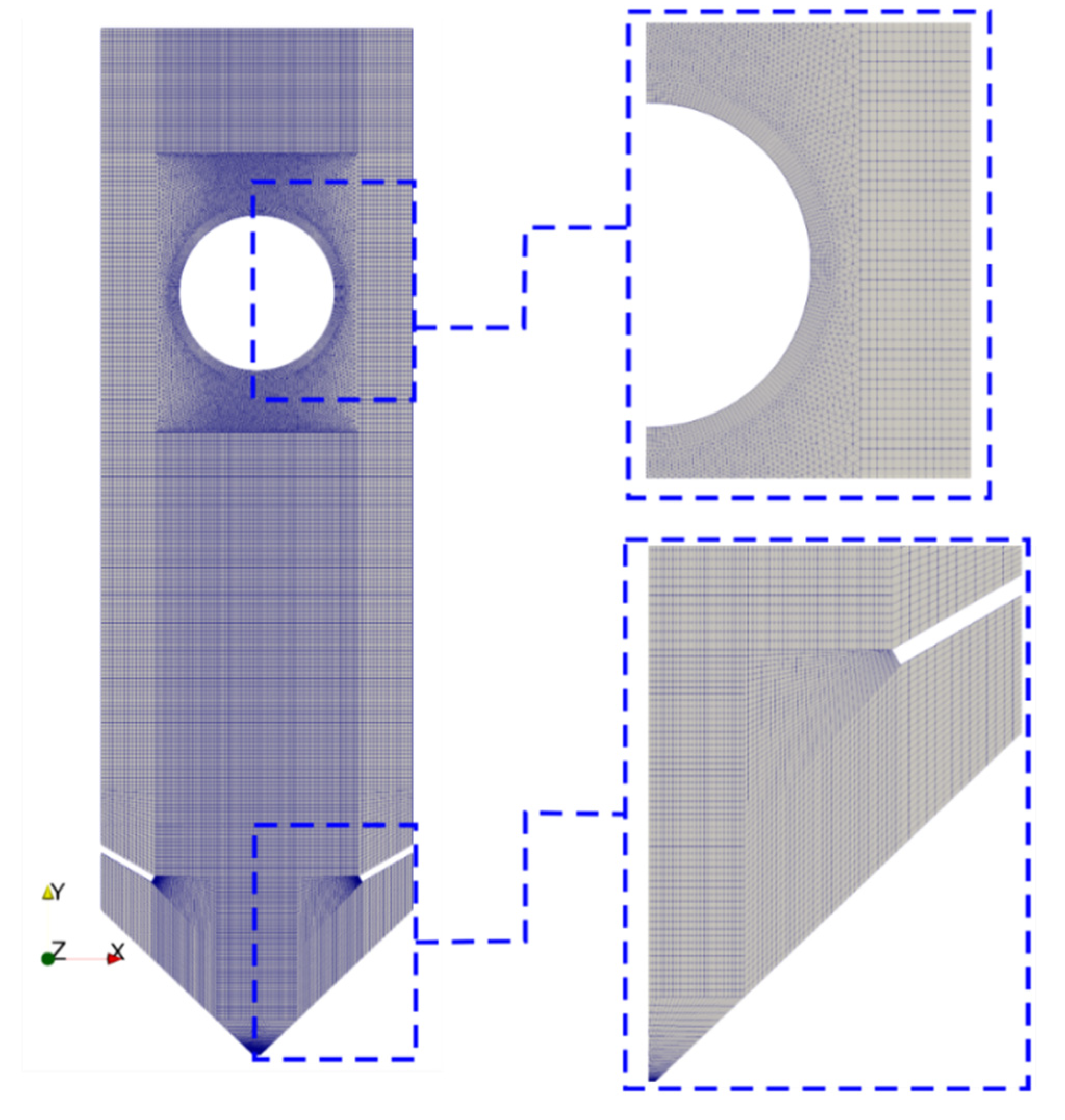
The geometry and computational mesh for the CFD simulations were built within the open-source software Gmsh©, version 4.6.0. To accurately simulate the highly expanded and turbulent gas jets in the grinding region, a high spatial and temporal numerical resolution is required. Thus, taking into consideration the computational demands, a hybrid 2D computational mesh, comprised of a suitable mesh refinement at the grinding region, was used. Since OpenFOAM® can only import 3D models, a 3D mesh with a unit thickness in the z-direction was generated and the solver was set to not calculate in this direction for the case of 2D simulations.
The grid lines were aligned with the nozzles’ flow to avoid numerical diffusion, and fine grid size were used at the nozzles’ inlet boundaries—the nozzle diameter (2.4 mm) was represented by at least 30 computational cells—to guarantee an accurate simulation of the nozzles’ flow (gas jets). Figure 2 depicts the computational mesh along with some quality parameters.
For pressure-velocity coupling, the PIMPLE algorithm, which is a combination of the SIMPLE (Semi-Implicit Method for Pressure-Linked Equations) and PISO (Pressure-Implicit with Split-Operator) algorithms, was used [33]. Second-order discretization schemes were applied for numerical discretization of all transport equations (divergence, Laplacian, and gradient terms). The first-order-bounded implicit Euler scheme was used for all unsteady terms (i.e., temporal discretization).
In this work, a time step of about 10−8 s was adopted in all simulations. The steady-state condition (periodic behavior of the flow properties) was reached after approximately 2 s. The convergence criteria for pressure, velocities, granular temperature, volume fractions, enthalpy, and kf-εf variables were set to 10−6, 10−8, 10−6, 10−9, 10−6, and 10−5, respectively. Even though an implicit scheme was used, the Courant-Friedrich-Levy number (CFL) was kept less than 0.5 for a time-accurate solution.
No-slip wall boundary conditions were used for both fluid and solid phases. Suitable wall functions were used to bridge the region between the wall and the fully turbulent region. A rotating wall boundary condition was applied at the classifier wall (rotation speed of 12,500 rpm, corresponding to a particle cut size less than the particle diameter used herein) which was comprised of 30 evenly spaced vanes. Only the air flow was able to leave the equipment through the gaps between the vanes in the classifier (batch condition).
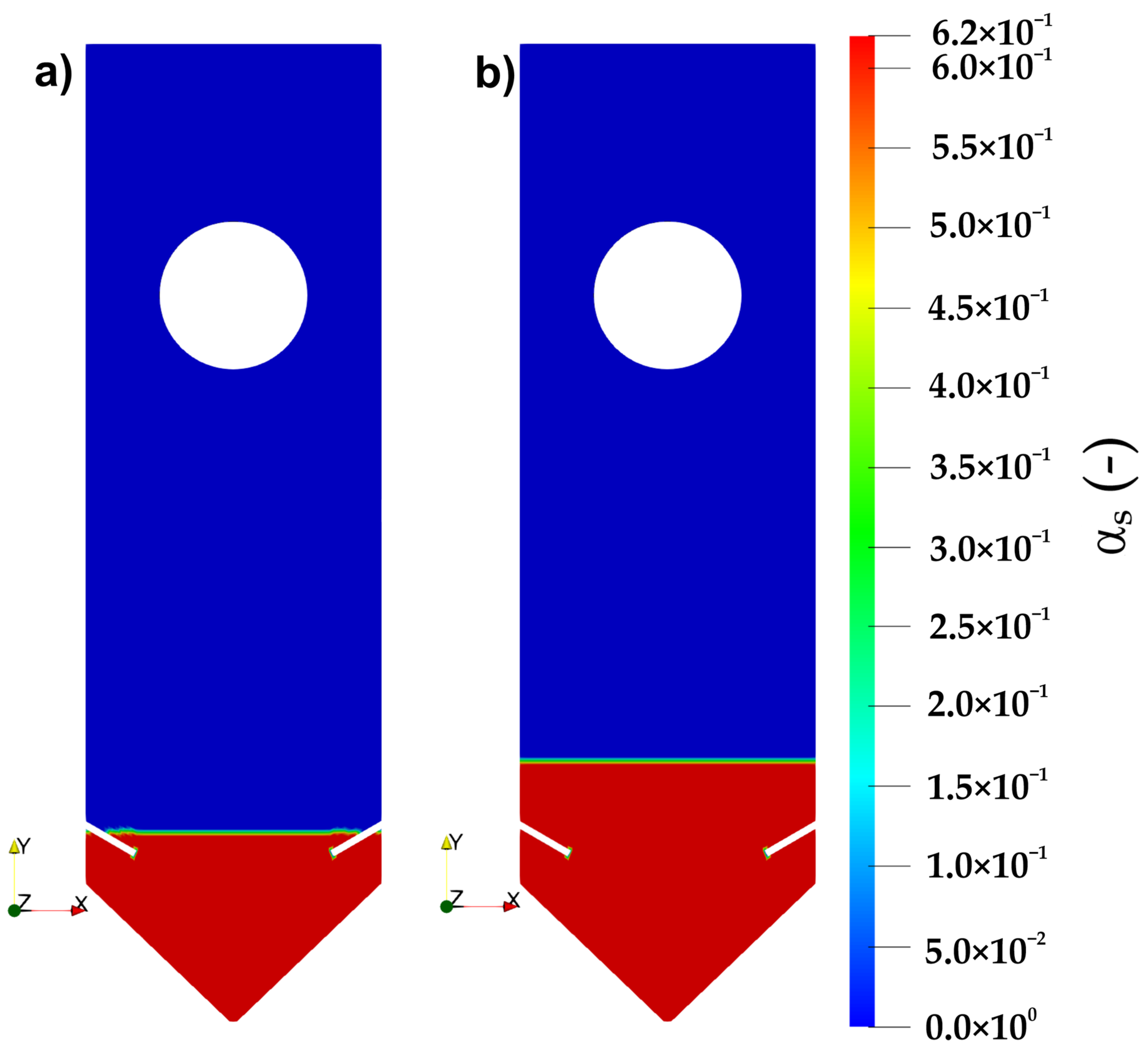
For the solid holdup, two different values were used: 400 g and 700 g. Those masses corresponded to the initial particle bed heights shown in Figure 3a,b, respectively, for the Euler–Euler simulations.
The jet injection velocities of about 256.0 and 326.7 m/s, which correspond to Laval nozzle inlet pressures (gauge pressure) of 0.5 and 1 bar, respectively, were applied in the simulations. The nozzle outlet velocities were calculated according to
where vnozzle, T, R, M, pe, p, and γ are the velocity at the nozzle exit, the absolute temperature of the inlet gas, the universal gas law constant, the gas molecular mass, the absolute pressure at the nozzle exit, the absolute pressure of the inlet gas, and the isentropic expansion factor, respectively.
To calculate the volumetric particle velocity in the entire calculation domain (Vp_average), the following equation was used:
where ϑ, and Vp are the total calculation domain volume, and the local time-averaged particle velocity, respectively.
3. Results and Discussion
3.1. Influence of the Solid Holdup and the Nozzle Inlet Pressure on the Volumetric Average Particle Velocities
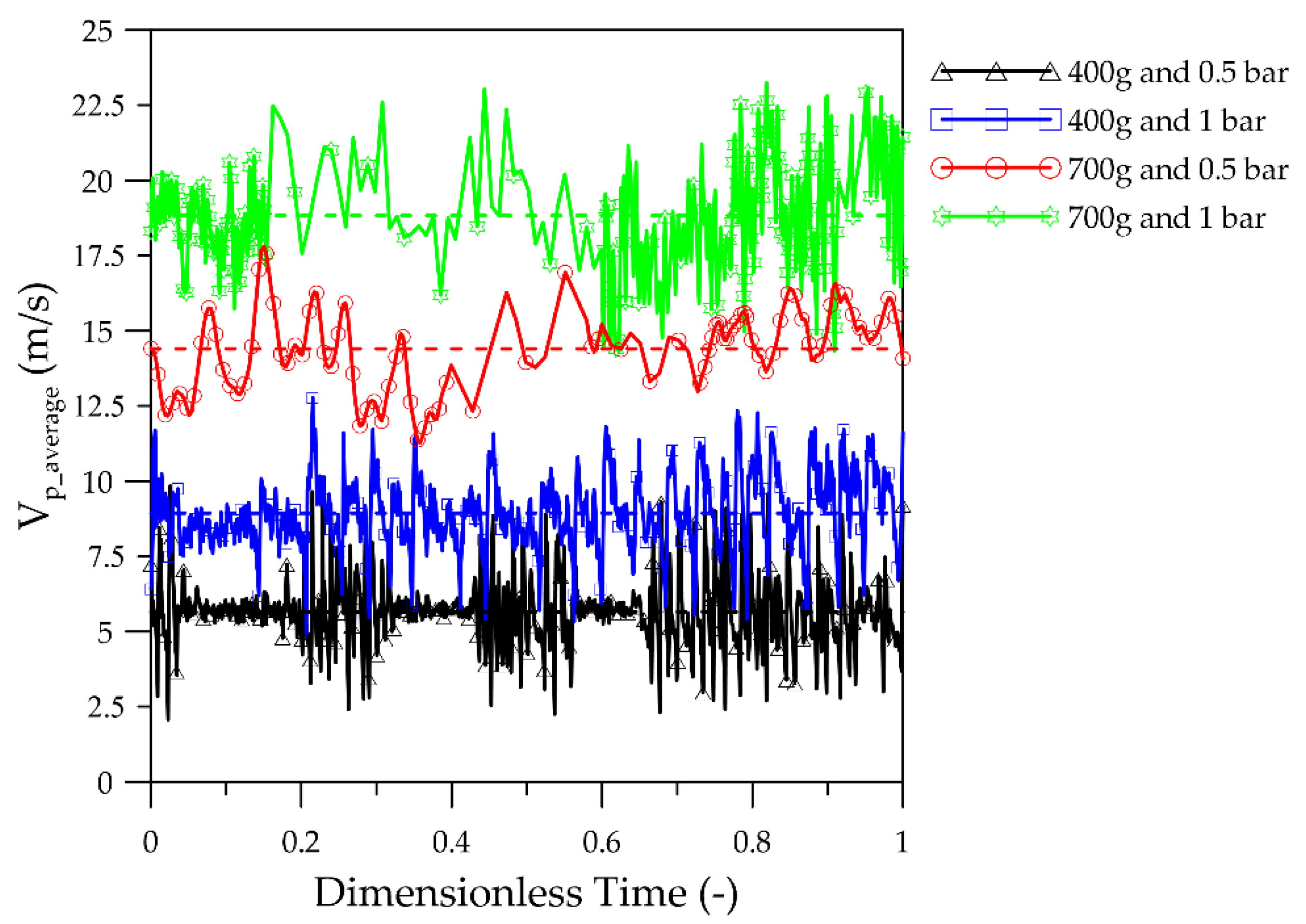
Due to the highly turbulent flow inside the fluidized bed opposed jet mill, a steady-state condition was considered herein to be established when the volumetric particle velocity, calculated by integrating the local particle velocity over the whole calculation domain (Equation (27)), reached a periodic behavior.
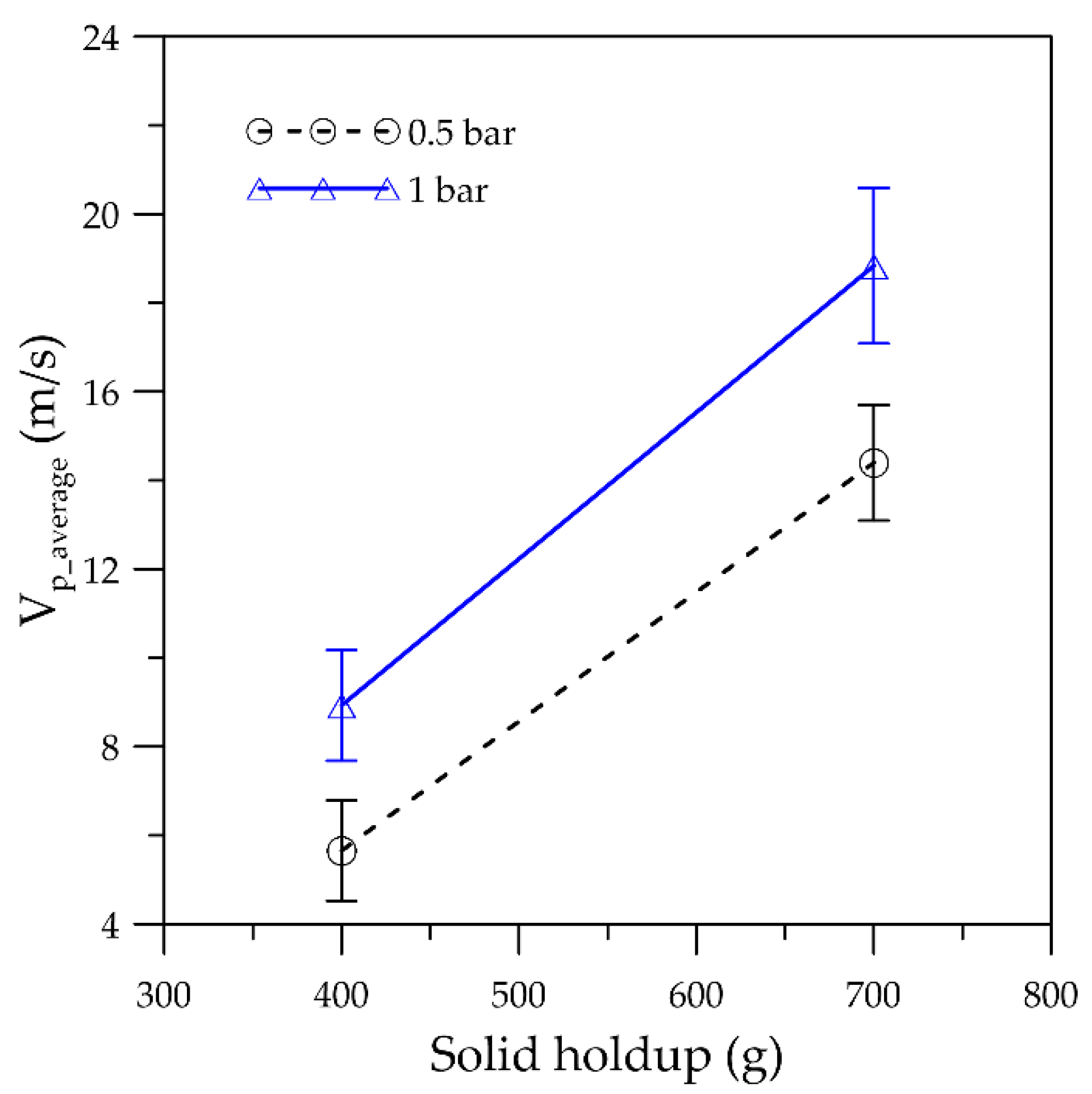
Figure 4 shows the temporal distribution of the volumetric particle velocity, under a periodic-behavior condition, as a function of the solid holdup and the nozzle inlet pressure. The corresponding time-averaged values are depicted in Figure 5.
As can been seen in Figure 4 and Figure 5, the volumetric average particle velocity increases with increasing both, the nozzle inlet air and the solids holdup. Since the curves in Figure 5 are approximately parallel, the increment in the solid holdup from 400 to 700 g caused a similar proportional increment in the volumetric particle velocity for both nozzle pressure values. Furthermore, the solid holdup effect on the volumetric particle velocity was shown to be more pronounced than the nozzle inlet effect, for the conditions investigated herein. These effects can be attributed to the complex particle–flow interaction in the grinding and transport regions, which will be explored in the next sections.
Strobel et al. [6] used ductile aluminum microspheres as tracers (particle probe method) to investigate the glass microspheres impact velocity in a batch fluidized bed opposed jet mill as a function of the solid holdup and the nozzle pressure. The glass microsphere diameter was the same as that used herein in the simulation (≈55 μm). Under a solid holdup of 400 g, the measured median impact velocity (Q50) was less than 10 m/s, regardless of the nozzle inlet pressure (0.5, 1, 2, and 3 bar). On the other hand, they did not observe significant influence of the solid holdup on the median impact velocity using the particle probe method but rather only on the distribution of contacts per probe particle. Furthermore, the authors claimed that, in all cases, the median impact velocity was much lower than the maximum speed in the expanding gas jets. It is worth mentioning that despite the Euler–Euler simulations give insights on the bulk particle–fluid flow rather than on the particle level, the volumetric average particle velocities calculated herein were similar to those reported in the literature.
3.2. Influence of the Solid Holdup and the Nozzle Inlet Pressure on the Time-Averaged Particle Volume Fraction Distribution
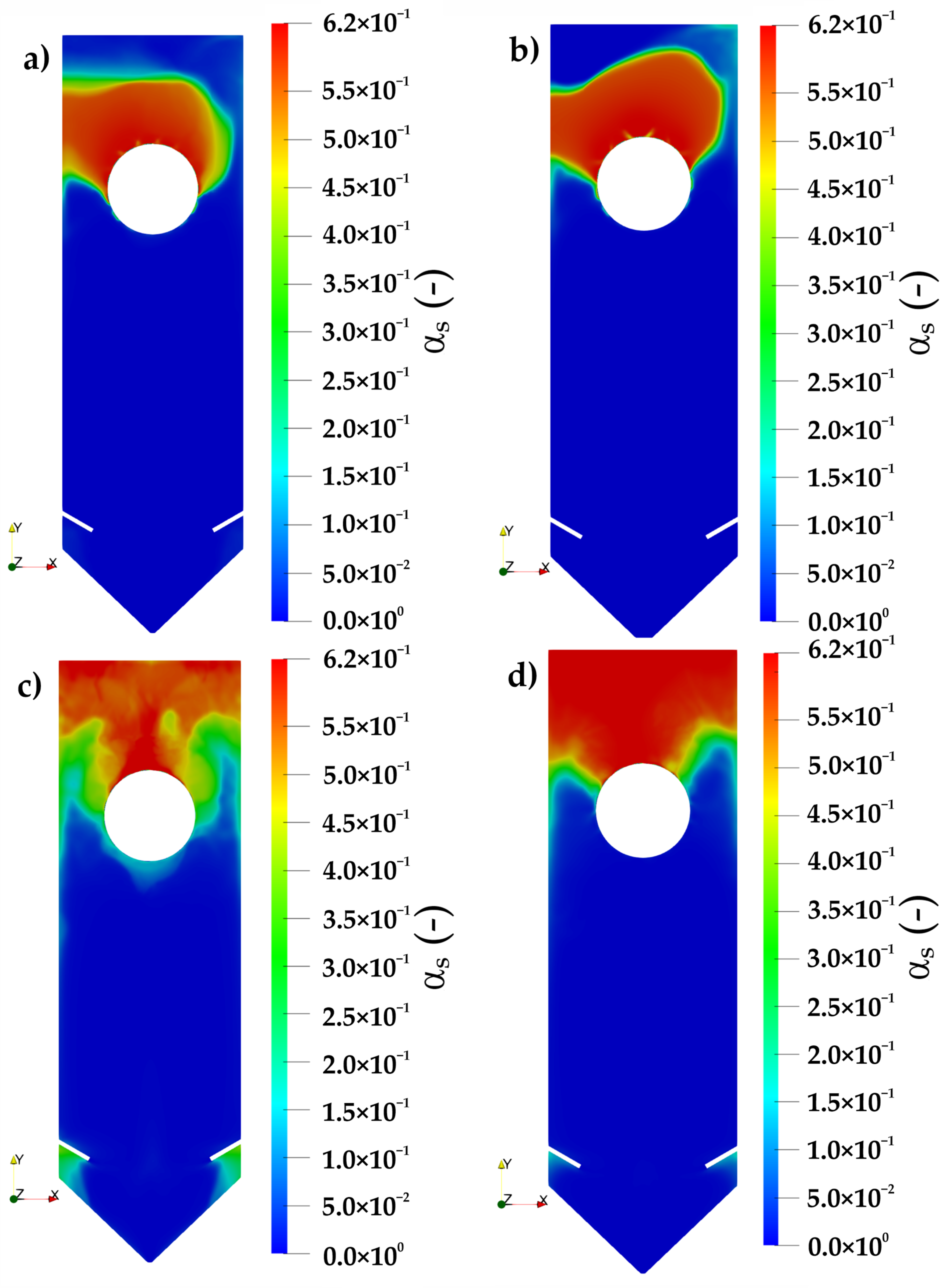
Figure 6 shows the time-averaged particle volume fraction distribution across the fluidized bed opposed jet mill as a function of the solid holdup (400 and 700 g) and the nozzle inlet pressure (0.5 and 1 bar).
It can be observed that, regardless of the solid holdup and nozzle inlet pressure, the highest values of particle concentration were found near the classifier wall (Figure 6). In the case of high solid holdup and low nozzle inlet pressure (Figure 6c), particles also tend to concentrate below the lateral nozzles. Additionally, the amount of solid accumulated in the classifier region increases with increasing either the solid holdup or the nozzle inlet pressure. Otherwise, the grinding and transport regions presented dilute solid volume fractions.
These numerical results are following the experimental observations reported by Köninger et al. [2], and Köninger et al. [3]. Using a high-speed camera, the authors revealed a remarkably high solid concentration near the classifier, which increased by increasing the solid holdup. According to the authors, increasing the particle concentration can increase the collision frequency and hence the particle agglomeration. The formation of particle cluster near the classifier strongly affect the classification performance and consequently the milling process efficiency. Therefore, a complete understanding of particle transport from the grinding region towards the classifier (transport region) is of fundamental importance.
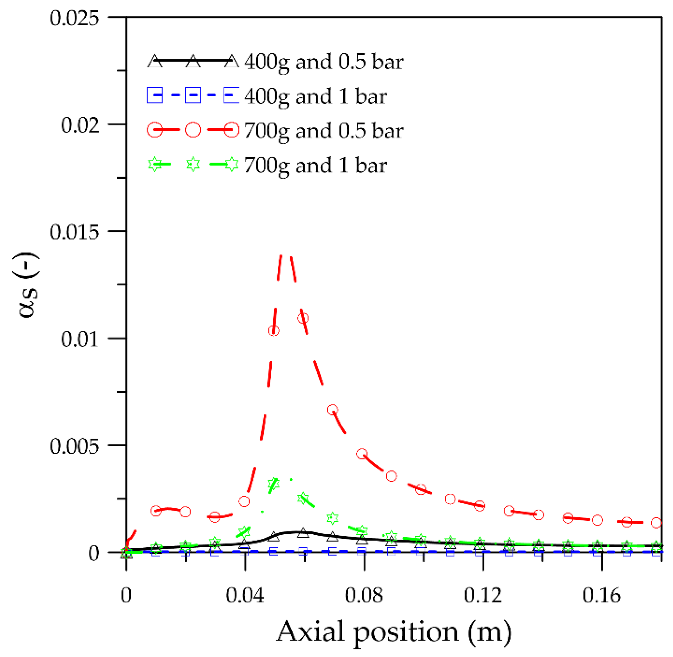
The time-averaged particle volume fraction plotted over the axial line at the center of the equipment, covering the grinding and the transporting regions, is shown in Figure 7.
As expected from Figure 6, very low solid volume fractions were observed over the axial position throughout the fluidized bed, with maximum values at the griding region that decreases towards the transport region (Figure 7).
The particle concentration in the grinding region increases with increasing the solid holdup and decreasing the nozzle inlet pressure, since higher grinding pressures reduce the particle residence time in the grinding region, dragging the particles upwards due to the action of more intense forces.
Therefore, the solid holdup and the nozzle inlet pressure can influence the solid concentration at the grinding region and the probability of particle–particle collisions, and more possible aggregation and breakage events. The maximum value of particle concentration was found for a high value of solid holdup combined with a low value of nozzle inlet pressure.
Similar qualitative behavior was also observed experimentally by Strobel et al. [6] that used a calibrated capacitance probe to measure the particle concentration distribution over the axial position in a fluidized bed opposed jet mill.
Köninger et al. [2], who experimentally studied the comminution of glass microspheres in a lab-scale fluidized bed opposed jet mill, reported that the grinding kinetics was strongly affected by the solid holdup. According to the authors, increasing the solid holdup led to an increase in the product mass flow rate with finer particles.
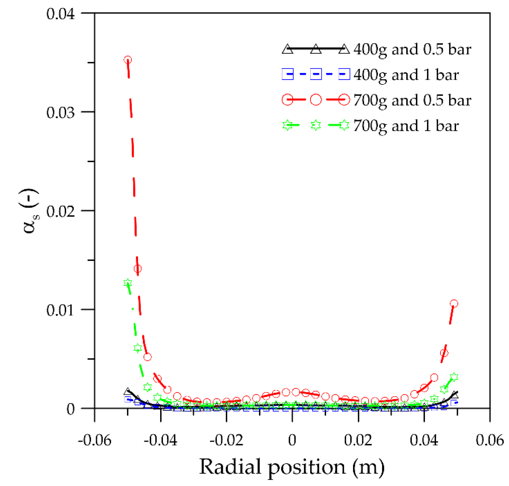
To further investigate the particle distribution inside the fluidized bed mill, Figure 8 depicts the radial distribution of the time-averaged particle volume fraction in the transport region at a fixed axial position of 0.145 m from the bottom of the fluidized bed.
Figure 8 shows that, regardless of the solid holdup and the nozzle inlet pressure values, the particle concentrations are low at the center and increase towards the fluidized bed wall forming a core-annulus flow. Similar to the axial distribution shown in Figure 7, an overall increase in the solid concentration is observed by increasing the solid holdup and decreasing the nozzle inlet pressure. Asymmetric behavior of the solid distribution can also be seen in Figure 7, which is intrinsic to a complex turbulent and compressible system such that found in a fluidized bed opposed jet mill.
The same qualitative trend was reported by Köninger et al. [2]. In this work, the particle concentration measurement, using a capacitance probe, was restricted only to one half of the equipment probably due to an assumption of symmetric flow behavior. The authors explained that the solid material not separated by the classifier wheel (below the cut size) is sent back to the grinding chamber along the fluidized bed wall and that the solid flow towards the classifier increases with increasing the solid holdup.
3.3. Analysis of the Particle–Fluid Dynamics Inside the Fluidized Bed Opposed Jet Mill
To shed new light on the complex particle–fluid behavior inside a fluidized bed gas opposed jet mill, the time-averaged velocity, the time-averaged streamlines, and the time-averaged resultant velocity vector distributions of both phases are systematically analyzed in this section.
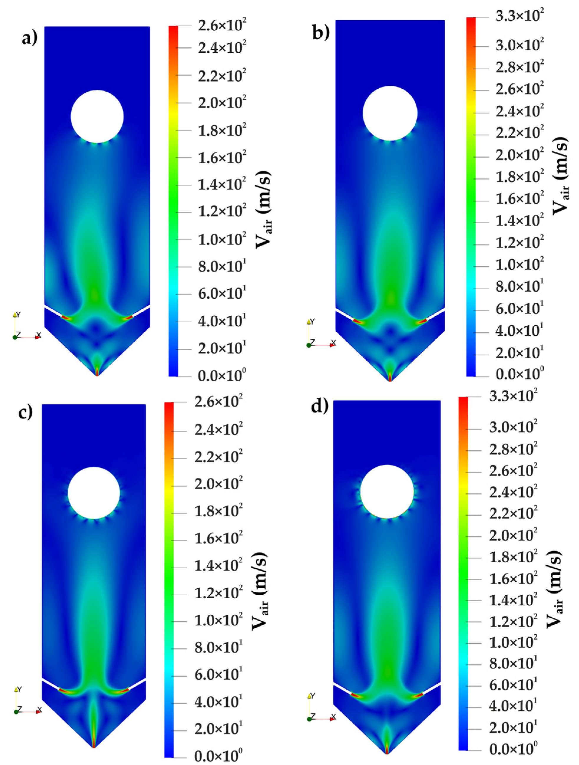
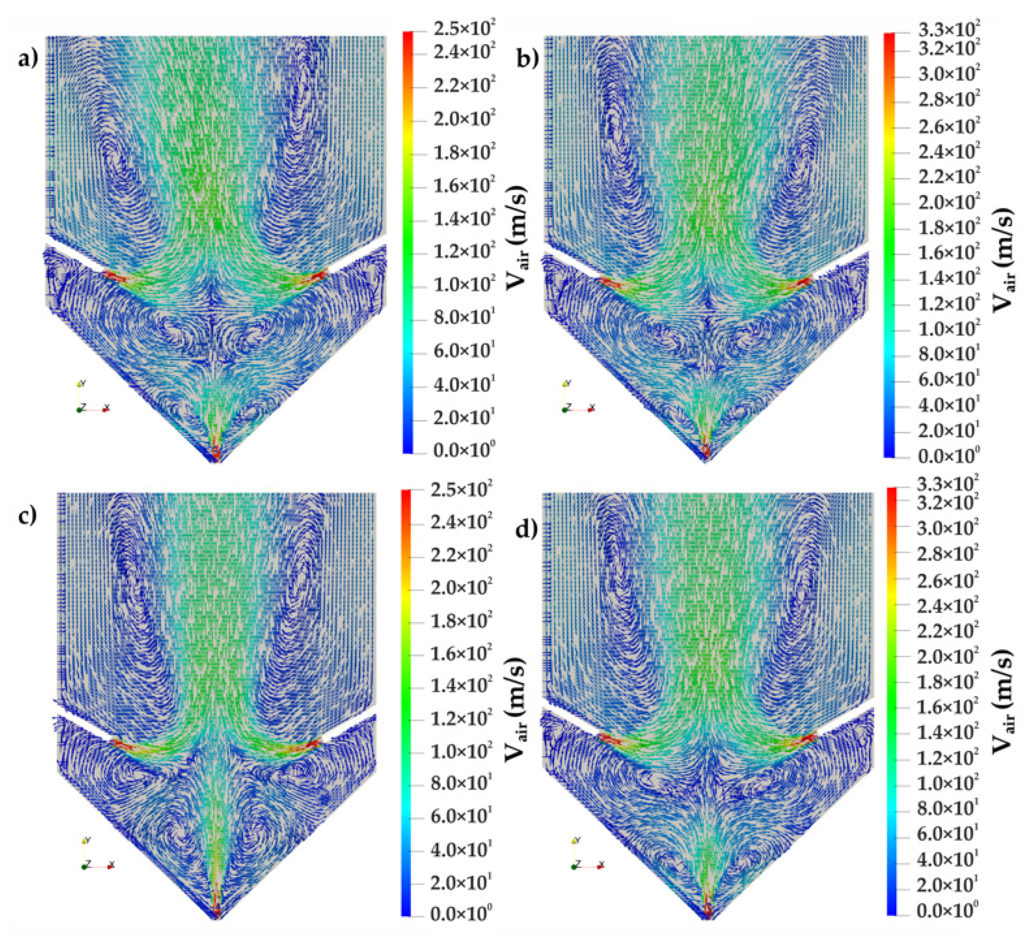
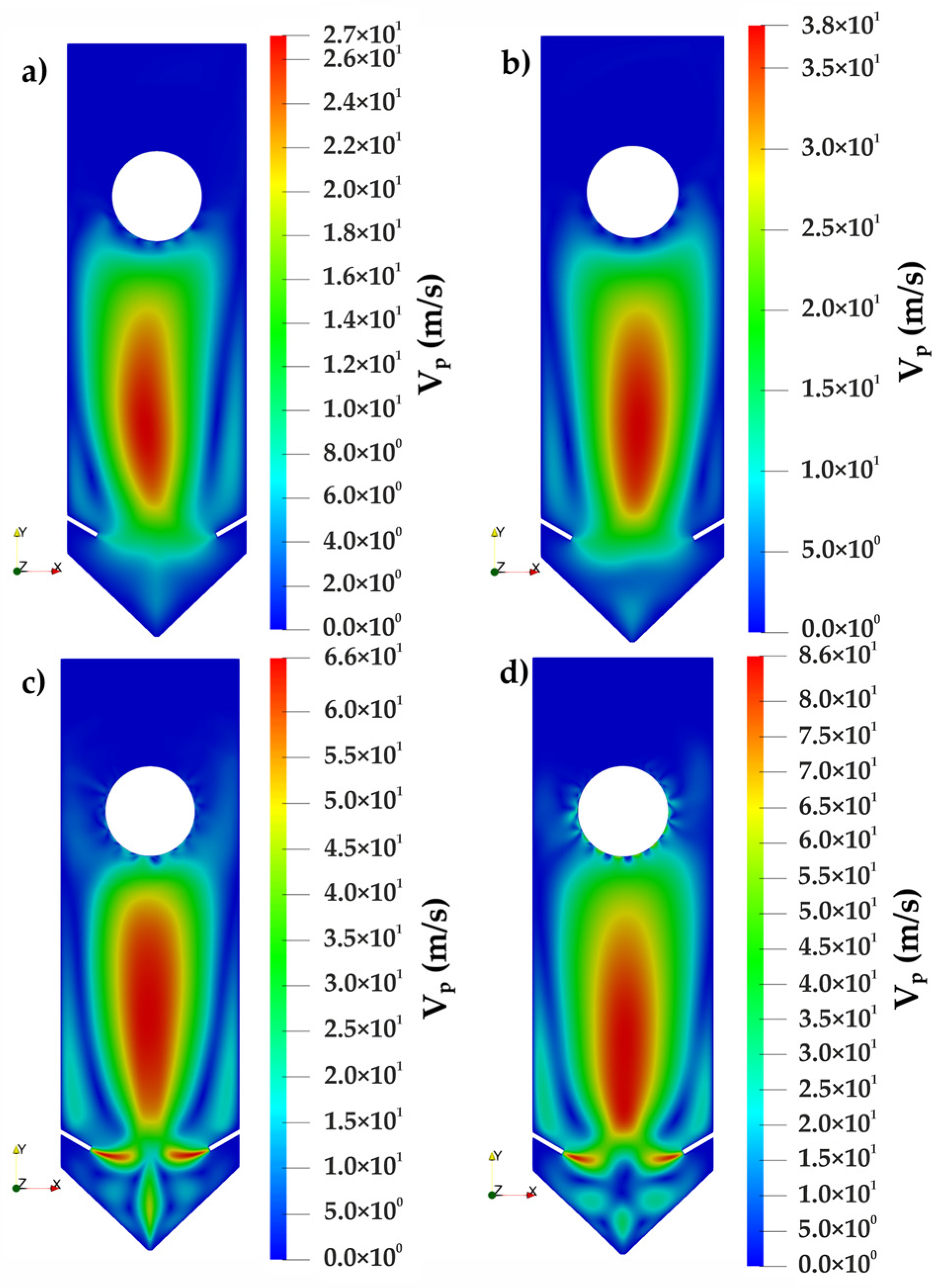
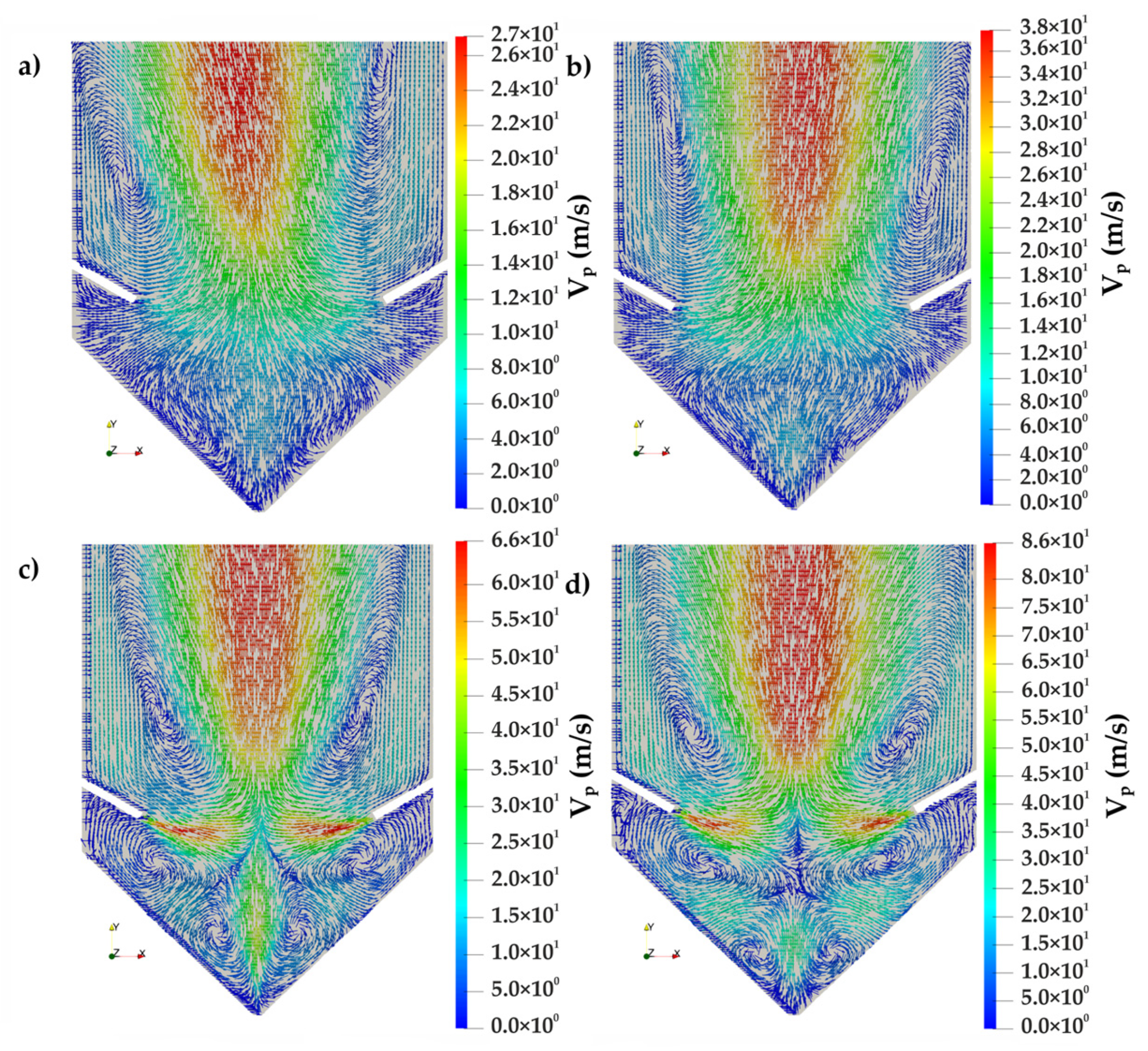
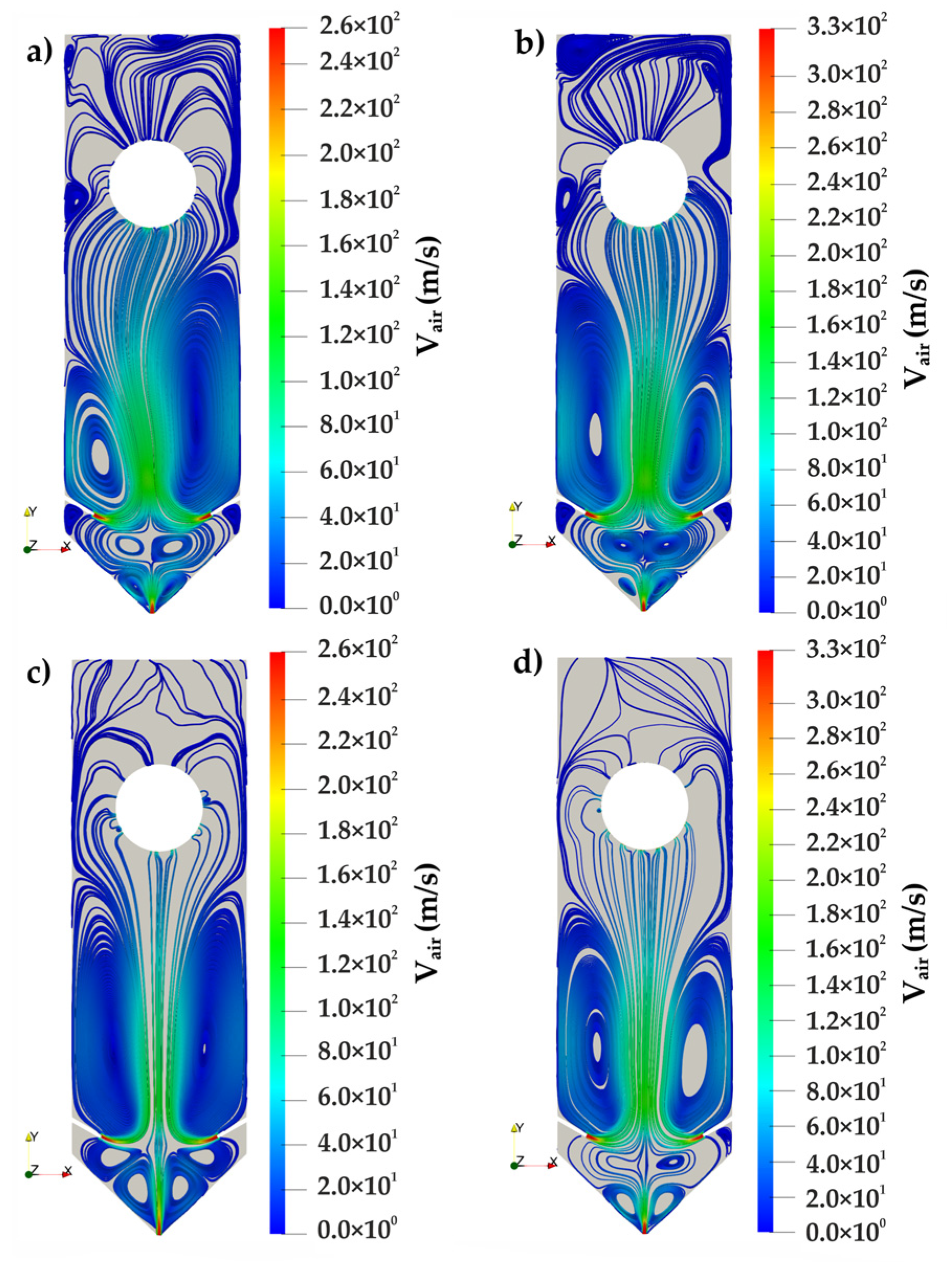
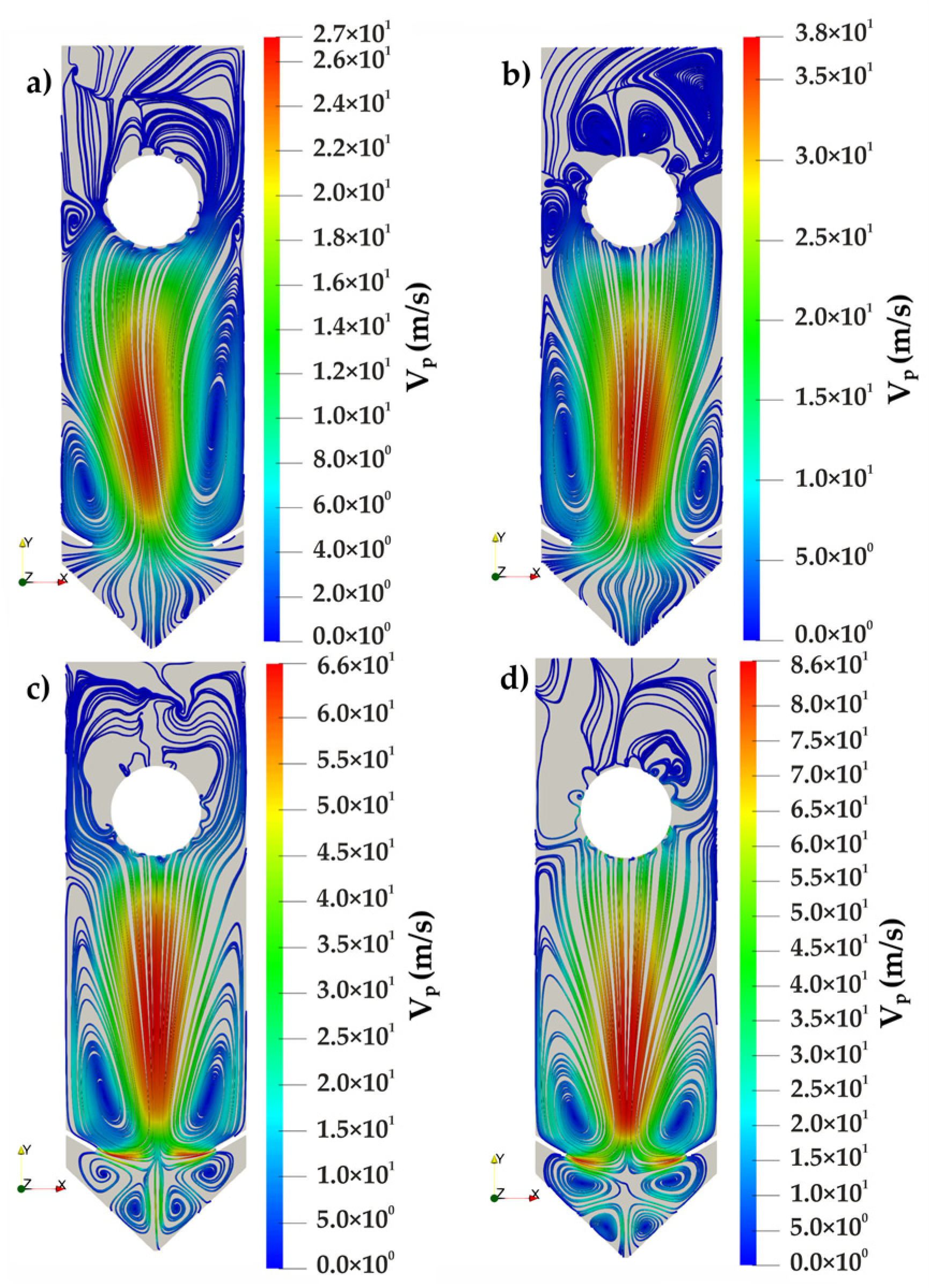
Figure 9, Figure 10, Figure 11 and Figure 12, show the velocity distribution and the resultant velocity vector fields for the air and particulate phases, respectively, for different combinations of solids holdup and nozzle inlet pressures.
As also observed by Strobel et al. [6] and Rajeswari et al. [14], the particle velocity is much lower than the air velocity, independently of the solids’ holdup and nozzle inlet pressure (Figure 9, Figure 10, Figure 11 and Figure 12). The highest values of the air velocity ranged from 260 to 330 m/s, whereas the corresponding values for the particles ranged from 27 to 86 m/s.
The jets from the nozzle and their focal point in the grinding region can be seen in detail in Figure 10 (air velocity vector fields), while the particle movement in the same region is depicted in Figure 12 (solid velocity vector fields). This region is characterized by a stressing zone where intense particle–particle collision take place and breakage may occur. As expected, the solids holdup and the nozzle pressure strongly affect the particle–fluid interaction in this region. Despite the highest values of solid holdup and nozzle pressure condition resulting in the overall highest values of particle velocity (Figure 12d), particle collisions seem to be strengthened by the contribution of the three nozzles’ jet in the effective formation of a focal point for particle collisions, as shown in Figure 12c. As can be seen in Figure 12a,b, the nozzle at the fluidized bed bottom does not effectively contribute to focalizing the particle flow. This behavior can also be seen in Figure 11, that shows the time-averaged particle velocity distribution in the apparatus.
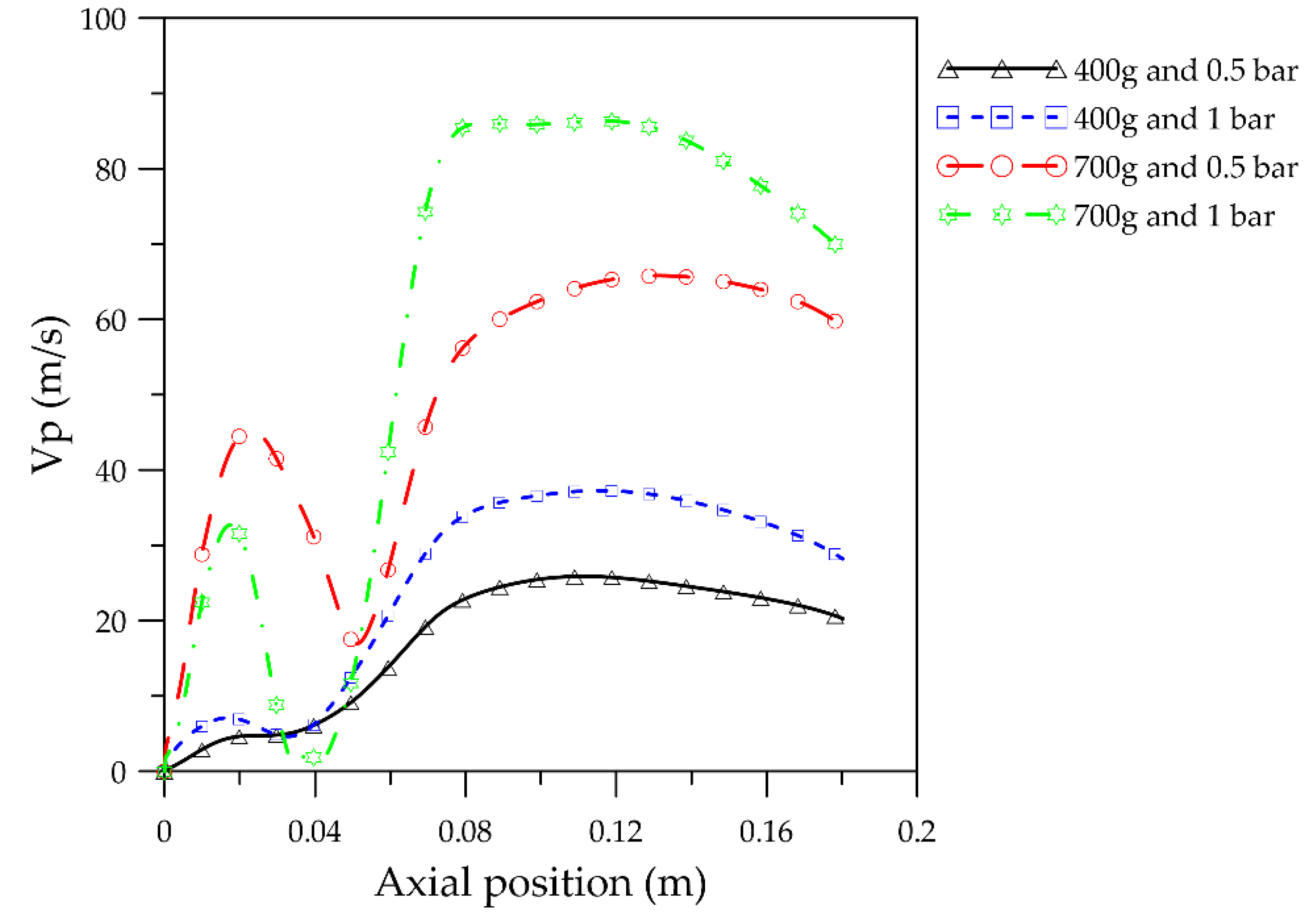
To further analyze this observation, Figure 13 presents the time-averaged particle velocity over the axial line along the center of the equipment, from the fluidized bed bottom (axial position equal to zero) to the transport region.
As previously observed, high solids holdups induced higher particle velocities in the grinding region (Figure 13). The highest value of particle velocity in the grinding region was observed for a solids holdup of 700 g and a nozzle inlet pressure of 0.5 bar, although the overall highest value of particle velocity was found for a solids holdup of 700 g and a nozzle inlet pressure of 1 bar in the transport region. On the one hand, higher particle velocity in the transport region than in the grinding region can lead to a higher rate of coarser products. On the other hand, higher particle velocity in the grinding region, which affects the kinetic energy during collisions and hence the breakage probability, lead to a higher rate of finer products.
The streamlines in Figure 14 and Figure 15 present the trajectories of the air and solid phases, respectively, where zones of fluid and particle recirculation can be identified.
Asymmetric behaviors of the particle and fluid flows can be seen in Figure 14 and Figure 15, which can directly affect the particle residence time in the grinding region and the transport of the particles towards the classifier. Interestingly, the more symmetric behavior was observed for a holdup of 700 g and a nozzle pressure of 0.5 bar (Figure 14c and Figure 15c).
As only the air can leave the equipment through the gaps between the classifier vanes (Figure 14 and Figure 15), particles are dragged from the grinding chamber towards the classifier and are recycled to the grinding region, since the classifier is considered herein to rotate with a particle cut size less than the particle diameter and are not discharged (Figure 15).
As can also be noted in Figure 15, the particles flow back to the griding region along the fluidized bed wall, which is in line with the experimental observations reported in the literature [2] and with the numerical results of the particle volume fraction distribution shown in the previous section, where high particle volume fractions were found to be at the fluidized bed wall (Figure 8).
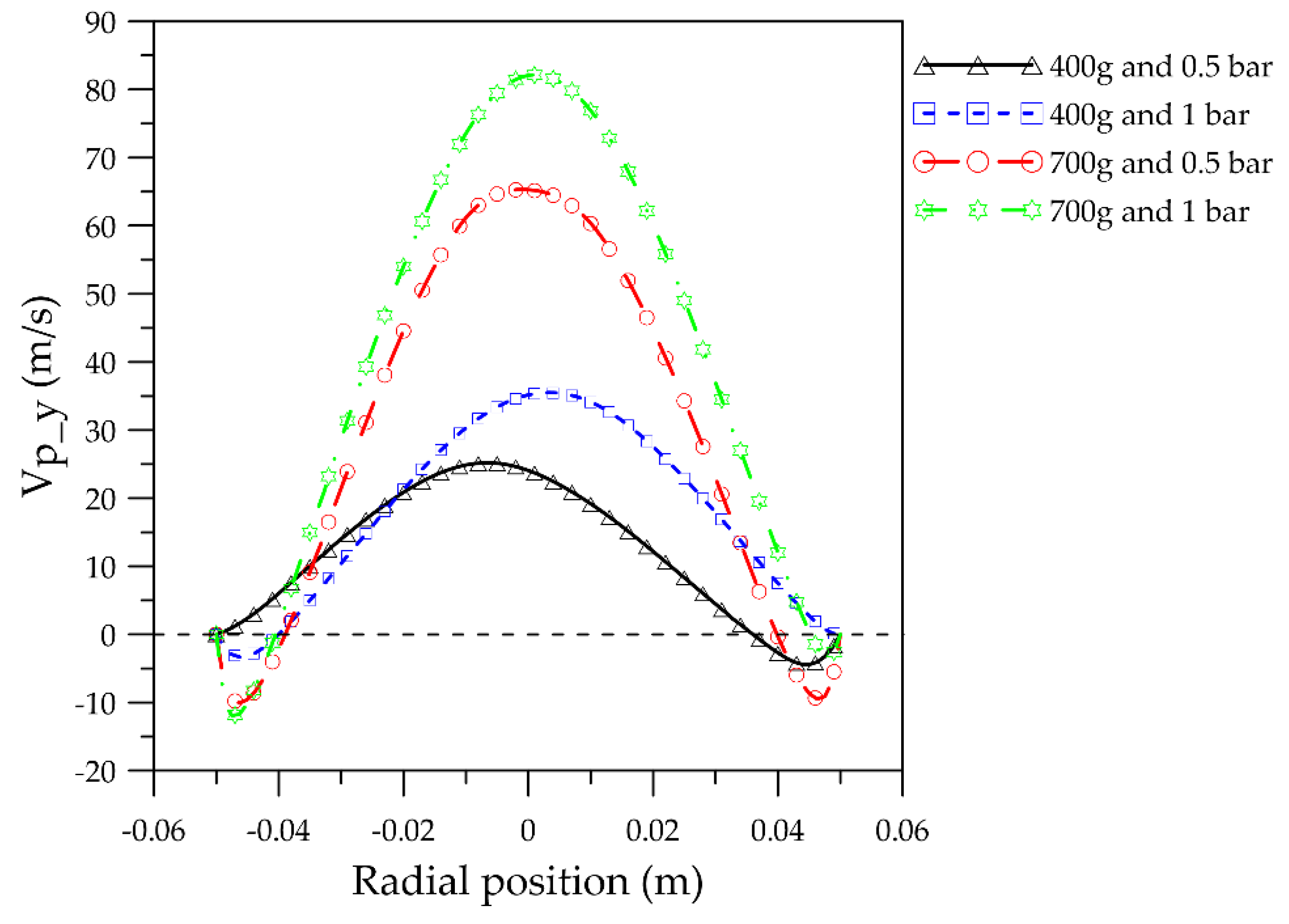
Figure 16 shows the radial distribution of the time-averaged y-component of the particle velocity (vertical direction) in the transport region at a fixed axial position of 0.145 m from the fluidized bed bottom. The maximum particle velocities were attained at the center of the fluidized bed (positive values) whereas negative values were found at the wall indicating that particles are flowing back to the grinding region along the wall, as previously discussed (Figure 16).
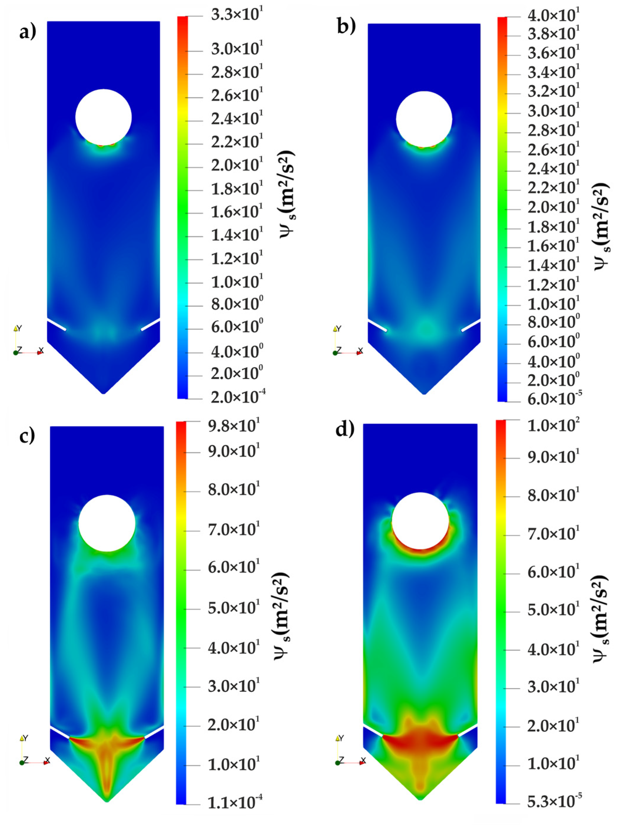
Finally, the granular temperature distribution, which comprises an important characterization of the particle velocity fluctuations [34] and can indicate the regions inside the fluidized bed jet mill under intense particle–particle interactions, is shown in Figure 17 for different conditions of solids holdup and nozzle inlet pressure.
In general, the highest particle–particle interactions (higher granular temperatures) were observed in the grinding region, mainly for the cases of high solids holdup (Figure 17). For the case of a solids holdup of 700 g and a nozzle inlet pressure of 0.5 bar, the high particle–particle interactions seem to be exclusively promoted by the nozzles’ air jets (Figure 17c), whereas for the same solids holdup but rather for a nozzle inlet pressure of 1 bar, the equipment walls at the grinding chamber, cylinder part, and classifier bottom, strongly affected the particle–particle interactions. Furthermore, a significant particle–particle interaction can also be seen during the particle flow in the transporting region. Therefore, depending on the operating conditions, not only the air jets but also the equipment walls can significantly contribute to the particle breakage and to comminution process performance.
4. Conclusions
The Euler–Euler approach along with the kinetic theory of granular flow and frictional models was applied to systematically investigate gas–solid multiphase flow inside an opposed gas jet fluidized bed. Using this approach, the solids movement and concentration within the apparatus under different operating conditions were modeled. The main conclusions are:
- Simulation results are in qualitative agreement with respect to published experimental results, not just in terms of movement and distribution but also with respect to particle collision velocity. The significant influence of the classifier on solids movement observed in operation of these mills was also observed in the model. This enables further study on solids flow around the classifier and determine process limits of classification with respect to solids over-loading and decreases process performance;
- Furthermore, asymmetric behavior of the particle and fluid flows were observed, indicating spatial and temporal periodic behavior within the apparatus. These oscillations may affect the particle residence time and stressing conditions in the grinding region and the transport of the particles towards the classifier. Onset and magnitude of these oscillations can be investigated by the proposed model, utilizing methods from system dynamics, leading to regime maps that may be linked to product properties;
- Apart from the particle–particle interactions in the grinding region, significant particle–particle interactions at the walls of the grinding chamber, the cylindrical lateral’s wall, and the classifier’s wall were observed, indicating that not only the air jets but also the equipment walls are contributing to particle breakage and comminution efficiency.
Future work will focus on the solids movement and distribution of polydisperse particles and explicitly consider size reduction by breakage. Furthermore, an in-depth study of solids concentration and movement in the vicinity of the classifier will be performed, with the aim of elucidating the effect of solids on operation and efficiency of the classifier.
Author Contributions
Conceptualization, D.A.d.S. and A.B.; Data curation, D.A.d.S.; Formal analysis, D.A.d.S.; Funding acquisition, D.A.d.S. and A.B.; Investigation, D.A.d.S. and S.B.; Methodology, D.A.d.S.; Project administration, D.A.d.S.; Resources, D.A.d.S. and A.B.; Software, D.A.d.S.; Supervision, D.A.d.S. and A.B.; Validation, D.A.d.S., S.B. and A.B.; Visualization, D.A.d.S.; Writing—original draft, D.A.d.S.; Writing—review & editing, D.A.d.S. and A.B. All authors have read and agreed to the published version of the manuscript.
Funding
This research was funded by CAPES (Brazilian Research Foundation) and the Alexander-von-Humboldt Foundation (process number 88881.312913/2018-01), which the authors gratefully acknowledge. We acknowledge support by Deutsche Forschungsgemeinschaft and Friedrich-Alexander-Universität Erlangen-Nürnberg (FAU) within the funding program Open Access Publishing.
Conflicts of Interest
The authors declare no conflict of interest.
References
- Wang, Y.; Peng, F. Parameter effects on dry fine pulverization of alumina particles in a fluidized bed opposed jet mill. Powder Technol. 2011, 214, 269–277. [Google Scholar] [CrossRef]
- Köninger, B.; Hensler, T.; Romeis, S.; Peukert, W.; Wirth, K.-E. Dynamics of fine grinding in a fluidized bed opposed jet mill. Powder Technol. 2018, 327, 346–357. [Google Scholar] [CrossRef]
- Köninger, B.; Spoetter, C.; Romeis, S.; Weber, A.P.; Wirth, K.-E. Classifier performance during dynamic fine grinding in fluidized bed opposed jet mills. Adv. Powder Technol. 2019, 30, 1678–1686. [Google Scholar] [CrossRef]
- Köninger, B.; Kögl, T.; Hensler, T.; Arlt, W.; Wirth, K.-E. Solid distribution in fluidized and fixed beds with horizontal high speed gas jets. Powder Technol. 2018, 336, 57–69. [Google Scholar] [CrossRef]
- Köninger, B.; Hensler, T.; Schug, S.; Arlt, W.; Wirth, K.-E. Horizontal secondary gas injection in fluidized beds: Solid concentration and velocity in multiphase jets. Powder Technol. 2017, 316, 49–58. [Google Scholar] [CrossRef]
- Strobel, A.; Köninger, B.; Romeis, S.; Schott, F.; Wirth, K.-E.; Peukert, W. Assessing stress conditions and impact velocities in fluidized bed opposed jet mills. Particuology 2020. [Google Scholar] [CrossRef]
- Jiang, Z.; Hagemeier, T.; Bück, A.; Tsotsas, E. Color-PTV measurement and CFD-DEM simulation of the dynamics of poly-disperse particle systems in a pseudo-2D fluidized bed. Chem. Eng. Sci. 2018, 6, 115–132. [Google Scholar] [CrossRef]
- Benedito, W.M.; Duarte, C.R.; Barrozo, M.A.S.; Santos, D.A. An investigation of CFD simulations capability in treating non-sphericalparticle dynamics in a rotary drum. Powder Technol. 2018, 332, 171–177. [Google Scholar] [CrossRef]
- Lun, C.K.K.; Savage, S.B.; Jeffrey, D.J.; Chepurniy, N. Kinetic theories for granular flow: Inelastic particles in coquette flow and singly inelastic particles in a general flow field. J. Fluid Mech. 1984, 140, 223–256. [Google Scholar] [CrossRef]
- Zhou, Z.Y.; Kuang, S.B.; Chu, K.W.; Yu, A.B. Discrete particle simulation of particle–fluid flow: Model formulations and their applicability. J. Fluid Mech. 2010, 661, 482–510. [Google Scholar] [CrossRef]
- Lin, W.; Guoli, Q.; Ming, T.; Xuemin, L.; Hassan, M.; Huilin, L. Simulated pulsed flow of gas and particles in a horizontal oppose-pulsed gas jets of bubbling fluidized bed. Adv. Powder Technol. 2018, 29, 3507–3519. [Google Scholar] [CrossRef]
- Santos, D.A.; Alves, G.C.; Duarte, C.R.; Barrozo, M.A.S. Disturbances in the Hydrodynamic Behavior of a Spouted Bed Caused by an Optical Fiber Probe: Experimental and CFD Study. Ind. Eng. Chem. Res. 2012, 51, 3801–3810. [Google Scholar] [CrossRef]
- Shi, P.; Rzehak, R. Solid-liquid flow in stirred tanks: Euler-Euler/RANS modeling. Chem. Eng. Sci. 2020, 227, 1–23. [Google Scholar] [CrossRef]
- Rajeswari, M.S.R.; Azizli, K.A.M.; Hashim, S.F.S.; Abdullah, M.K.; Mujeebu, M.A.; Abdullah, M.Z. CFD simulation and experimental analysis of flow dynamics and grinding performance of opposed fluidized bed air jet mill. Int. J. Miner. Process. 2011, 98, 94–105. [Google Scholar] [CrossRef]
- Lee, H.W.; Song, S.; Kim, H.T. Improvement of pulverization efficiency for micro-sized particles grinding by uncooled high-temperature air jet mill using a computational simulation. Chem. Eng. Sci. 2019, 207, 1140–1147. [Google Scholar] [CrossRef]
- Teng, S.; Wang, P.; Zhu, L.; Young, M.-W.; Gogos, C.G. Experimental and numerical analysis of a lab-scale fluid energy mill. Powder Technol. 2009, 195, 31–39. [Google Scholar] [CrossRef]
- Teng, S.; Wang, P.; Zhang, Q.; Gogos, C. Analysis of Fluid Energy Mill by gas-solid two-phase flow simulation. Powder Technol. 2011, 208, 684–693. [Google Scholar] [CrossRef]
- Brosh, T.; Kalman, H.; Levy, A.; Peyron, I. Francois R. DEM-CFD simulation of particle comminution in jet-mill. Powder Technol. 2014, 257, 104–112. [Google Scholar] [CrossRef]
- Rodnianski, V.; Levy, A.; Kalman, H. A new method for simulation of comminution process in jet mills. Powder Technol. 2019, 343, 867–879. [Google Scholar] [CrossRef]
- Bnà, S.; Ponzini, R.; Cestari, M.; Cavazzoni, C.; Cottini, C.; Benassi, A. Investigation of particle dynamics and classification mechanism in a spiral jet mill through computational fluid dynamics and discrete element methods. Powder Technol. 2020, 364, 746–773. [Google Scholar] [CrossRef]
- Schaeffer, G. Instability in the evolution equations describing incompressible granular flow. J. Differ. Equ. 1987, 66, 19–50. [Google Scholar] [CrossRef] [Green Version]
- Johnson, P.C.; Jackson, R. Frictional-collisional constitutive relations for granular materials with application to plane shearing. J. Fluid Mech. 1987, 176, 67–93. [Google Scholar] [CrossRef]
- Gidaspow, D. Multiphase Flow and Fluidization. Continuum and Kinetic Theory Descriptions; Elsevier Science: San Diego, CA, USA, 1994; ISBN 978-0-08-051226-6. [Google Scholar] [CrossRef]
- Cokljat, D.; Ivanov, V.A.; Sarasola, F.J.; Vasquez, S.A. Multiphase k-epsilon Models for Unstructured Meshes. In ASME 2000 Fluids Engineering Division Summer Meeting; ASME: Boston, MA, USA, 2000; pp. 749–754. ISBN 0791819795. [Google Scholar]
- Elghobashi, S.E.; Abou-Arab, T.W. A two-equation turbulence model for two-phase flows. Phys. Fluids 1983, 26, 931–938. [Google Scholar] [CrossRef]
- Launder, B.E.; Spalding, D.B. The numerical computation of turbulent flows. Comput. Methods Appl. Mech. Eng. 1974, 3, 269–289. [Google Scholar] [CrossRef]
- Ranz, W.E.; Marshall, W.R. Evaporation from drops. Chem. Eng. Prog. 1952, 48, 141–146. [Google Scholar]
- Wen, C.Y.; Yu, Y.H. Mechanics of fluidization. Chem. Eng. Prog. 1966, 62, 100–111. [Google Scholar]
- Ergun, S. Fluid flow through packed columns. Chem. Eng. Prog. 1952, 48, 89–94. [Google Scholar]
- Batista, J.N.M.; Santos, D.A.; Béttega, R. Determination of the physical and interaction properties of sorghum grains: Application to computational fluid dynamics–discrete element method simulation of the fluid dynamics of a conical spouted bed. Particuology 2020. [Google Scholar] [CrossRef]
- Kobayashi, T.; Tanaka, T.; Shimada, N.; Kawaguchi, T. DEM-CFD analysis of fluidization behavior of Geldart Group A particles using a dynamic adhesion force model. Powder Technol. 2013, 248, 143–152. [Google Scholar] [CrossRef]
- Upadhyay, M.; Kim, A.; Kim, H.; Lim, D.; Lim, H. An Assessment of Drag Models in Eulerian-Eulerian CFD Simulation of Gas-Solid Flow Hydrodynamics in Circulating Fluidized Bed Riser. ChemEngineering 2020, 4, 37. [Google Scholar] [CrossRef]
- Barton, I.E. Comparison of SIMPLE- and PISO-type algorithms for transient flows. Int. J. Numer. Methods Fluids 1998, 26, 459–483. [Google Scholar] [CrossRef]
- Goldhirsch, I. Introduction to granular temperature. Powder Technol. 2008, 182, 130–136. [Google Scholar] [CrossRef]
Figure 1.
Scheme of the fluidized bed opposed gas jet mill considered in the numerical studies.

Figure 2.
Hybrid 2D computational mesh properties: 48,858 computational cells (34,906 hexahedral and 13,952 prisms cells); maximum aspect ratio of 6.57; maximum non-orthogonality of 48.42°, and a non-orthogonality average of 12.74°; maximum skewness of 1.44.
Figure 2.
Hybrid 2D computational mesh properties: 48,858 computational cells (34,906 hexahedral and 13,952 prisms cells); maximum aspect ratio of 6.57; maximum non-orthogonality of 48.42°, and a non-orthogonality average of 12.74°; maximum skewness of 1.44.

Figure 3.
Initial particle loading conditions in the Euler–Euler simulations: (a) solid holdup of 400 g, equivalent to an initial bed height of 0.064 m; (b) solid holdup of 700 g, equivalent to an initial bed height of 0.088 m.
Figure 3.
Initial particle loading conditions in the Euler–Euler simulations: (a) solid holdup of 400 g, equivalent to an initial bed height of 0.064 m; (b) solid holdup of 700 g, equivalent to an initial bed height of 0.088 m.

Figure 4.
Temporal distribution of the volumetric particle velocity (calculated through Equation (27)) as a function of the solid holdup and the nozzle inlet pressure.
Figure 4.
Temporal distribution of the volumetric particle velocity (calculated through Equation (27)) as a function of the solid holdup and the nozzle inlet pressure.

Figure 5.
Time-averaged volumetric particle velocity as a function of the solid holdup and the nozzle inlet pressure.
Figure 5.
Time-averaged volumetric particle velocity as a function of the solid holdup and the nozzle inlet pressure.

Figure 6.
Time-averaged particle volume fraction distribution as a function of the solid holdup and the nozzle inlet pressure: (a) 400 g and 0.5 bar; (b) 400 g and 1 bar; (c) 700 g and 0.5 bar; (d) 700 g and 1 bar.
Figure 6.
Time-averaged particle volume fraction distribution as a function of the solid holdup and the nozzle inlet pressure: (a) 400 g and 0.5 bar; (b) 400 g and 1 bar; (c) 700 g and 0.5 bar; (d) 700 g and 1 bar.

Figure 7.
Axial distribution of the time-averaged solid volume fraction at the center of the fluidized bed, from the fluidized bed bottom (axial position equal to zero) to the transporting region.
Figure 7.
Axial distribution of the time-averaged solid volume fraction at the center of the fluidized bed, from the fluidized bed bottom (axial position equal to zero) to the transporting region.

Figure 8.
Radial distribution of the time-averaged solid volume fraction at a fixed axial position of 0.145 m from the equipment bottom (transport region).
Figure 8.
Radial distribution of the time-averaged solid volume fraction at a fixed axial position of 0.145 m from the equipment bottom (transport region).

Figure 9.
Time-averaged air velocity distribution (resultant velocity) as a function of the solid holdup and the nozzle inlet pressure: (a) 400 g and 0.5 bar; (b) 400 g and 1 bar; (c) 700 g and 0.5 bar; (d) 700 g and 1 bar.
Figure 9.
Time-averaged air velocity distribution (resultant velocity) as a function of the solid holdup and the nozzle inlet pressure: (a) 400 g and 0.5 bar; (b) 400 g and 1 bar; (c) 700 g and 0.5 bar; (d) 700 g and 1 bar.

Figure 10.
Time-averaged resultant vectors distribution of air velocity near the grinding region as a function of the solid holdup and the nozzle inlet pressure: (a) 400 g and 0.5 bar; (b) 400 g and 1 bar; (c) 700 g and 0.5 bar; (d) 700 g and 1 bar.
Figure 10.
Time-averaged resultant vectors distribution of air velocity near the grinding region as a function of the solid holdup and the nozzle inlet pressure: (a) 400 g and 0.5 bar; (b) 400 g and 1 bar; (c) 700 g and 0.5 bar; (d) 700 g and 1 bar.

Figure 11.
Time-averaged particle velocity distribution (resultant velocity) as a function of the solid holdup and the nozzle inlet pressure: (a) 400 g and 0.5 bar; (b) 400 g and 1 bar; (c) 700 g and 0.5 bar; (d) 700 g and 1 bar.
Figure 11.
Time-averaged particle velocity distribution (resultant velocity) as a function of the solid holdup and the nozzle inlet pressure: (a) 400 g and 0.5 bar; (b) 400 g and 1 bar; (c) 700 g and 0.5 bar; (d) 700 g and 1 bar.

Figure 12.
Time-averaged resultant vectors distribution of particle velocity near the grinding region as a function of the solid holdup and the nozzle inlet pressure: (a) 400 g and 0.5 bar; (b) 400 g and 1 bar; (c) 700 g and 0.5 bar; (d) 700 g and 1 bar.
Figure 12.
Time-averaged resultant vectors distribution of particle velocity near the grinding region as a function of the solid holdup and the nozzle inlet pressure: (a) 400 g and 0.5 bar; (b) 400 g and 1 bar; (c) 700 g and 0.5 bar; (d) 700 g and 1 bar.

Figure 13.
Axial distribution of the time-averaged particle velocity at the center of the equipment, from the bottom nozzle to the lower wall of the classifier.
Figure 13.
Axial distribution of the time-averaged particle velocity at the center of the equipment, from the bottom nozzle to the lower wall of the classifier.

Figure 14.
Streamlines based on the time-averaged air velocity as a function of the solid holdup and the nozzle inlet pressure: (a) 400 g and 0.5 bar; (b) 400 g and 1 bar; (c) 700 g and 0.5 bar; (d) 700 g and 1 bar.
Figure 14.
Streamlines based on the time-averaged air velocity as a function of the solid holdup and the nozzle inlet pressure: (a) 400 g and 0.5 bar; (b) 400 g and 1 bar; (c) 700 g and 0.5 bar; (d) 700 g and 1 bar.

Figure 15.
Streamlines based on the time-averaged particle velocity as a function of the solid holdup and the nozzle inlet pressure: (a) 400 g and 0.5 bar; (b) 400 g and 1 bar; (c) 700 g and 0.5 bar; (d) 700 g and 1 bar.
Figure 15.
Streamlines based on the time-averaged particle velocity as a function of the solid holdup and the nozzle inlet pressure: (a) 400 g and 0.5 bar; (b) 400 g and 1 bar; (c) 700 g and 0.5 bar; (d) 700 g and 1 bar.

Figure 16.
Radial distribution of the time-averaged particle velocity at a fixed axial position of 0.145 m from the equipment bottom (transport region).
Figure 16.
Radial distribution of the time-averaged particle velocity at a fixed axial position of 0.145 m from the equipment bottom (transport region).

Figure 17.
Time-averaged granular temperature distribution as a function of the solid holdup and the nozzle inlet pressure: (a) 400 g and 0.5 bar; (b) 400 g and 1 bar; (c) 700 g and 0.5 bar; (d) 700 g and 1 bar.
Figure 17.
Time-averaged granular temperature distribution as a function of the solid holdup and the nozzle inlet pressure: (a) 400 g and 0.5 bar; (b) 400 g and 1 bar; (c) 700 g and 0.5 bar; (d) 700 g and 1 bar.


Table 1.
Geometric parameters of the fluidized bed opposed jet mill unit according to Figure 1.
Table 1.
Geometric parameters of the fluidized bed opposed jet mill unit according to Figure 1.
| Parameter | Value | Parameter | Value | Parameter | Value |
|---|---|---|---|---|---|
| L1 | 0.1985 m | L4 | 0.0654 m | D2 | 0.0500 m |
| L2 | 0.0465 m | L5 | 0.0850 m | θ | 30° |
| L3 | 0.0662 m | D1 | 0.1000 m | Dnozzle (exit) | 2.4 mm |
Table 2.
Constitutive equations for the Euler–Euler approach formulation.
| Constitutive Equations: | |
|---|---|
| Viscous stress tensor of the fluid phase: | (5) |
| Viscous stress tensor of the solid phase: | (6) |
| Total granular viscosity: | (7) |
| Kinetic () and collisional () granular viscosity: | (8) |
| (9) | |
| Frictional viscosity (Schaeffer’s model [21]): | (10) |
| Total granular pressure: | (11) |
| Kinetic () and collisional () granular pressure: | (12) |
| Frictional pressure (Johnson and Jackson’s model [22]): | (13) |
| Radial distribution function: | (14) |
| Solid bulk viscosity: | (15) |
| Conductivity of granular temperature: | (16) |
| Kinetic energy dissipation due to inelastic collisions: | (17) |
| Kinetic energy dissipation due to fluid friction: | (18) |
| Solid–gas momentum exchange coefficient (Gidaspow’s model [23]): | |
| (19) | |
| (20) | |
| (21) |
Publisher’s Note: MDPI stays neutral with regard to jurisdictional claims in published maps and institutional affiliations. |
© 2020 by the authors. Licensee MDPI, Basel, Switzerland. This article is an open access article distributed under the terms and conditions of the Creative Commons Attribution (CC BY) license (http://creativecommons.org/licenses/by/4.0/).
Share and Cite
MDPI and ACS Style
Araújo dos Santos, D.; Baluni, S.; Bück, A. Eulerian Multiphase Simulation of the Particle Dynamics in a Fluidized Bed Opposed Gas Jet Mill. Processes 2020, 8, 1621. https://doi.org/10.3390/pr8121621
AMA Style
Araújo dos Santos D, Baluni S, Bück A. Eulerian Multiphase Simulation of the Particle Dynamics in a Fluidized Bed Opposed Gas Jet Mill. Processes. 2020; 8(12):1621. https://doi.org/10.3390/pr8121621
Chicago/Turabian StyleAraújo dos Santos, Dyrney, Shivam Baluni, and Andreas Bück. 2020. "Eulerian Multiphase Simulation of the Particle Dynamics in a Fluidized Bed Opposed Gas Jet Mill" Processes 8, no. 12: 1621. https://doi.org/10.3390/pr8121621
Note that from the first issue of 2016, this journal uses article numbers instead of page numbers. See further details here.