Reliable Long-Term Data from Low-Cost Gas Sensor Networks in the Environment †
by
 , ,
, ,
Georgia Miskell
1, 
Jennifer Salmond
2,
Stuart Grange
1,
Lena Weissert
1,
Geoff Henshaw
3 and
David Williams
1,* 1
School of Chemical Sciences, University of Auckland, Auckland, New Zealand
2
School of Environment, University of Auckland, Auckland, New Zealand
3
Aeroqual Ltd., Auckland, New Zealand
*
Author to whom correspondence should be addressed.
†
Presented at the Eurosensors 2017 Conference, Paris, France, 3–6 September 2017.
Proceedings 2017, 1(4), 400; https://doi.org/10.3390/proceedings1040400
Published: 25 August 2017
(This article belongs to the Proceedings of Proceedings of Eurosensors 2017, Paris, France, 3–6 September 2017)
Abstract
:This poster examines long-term performance of low-cost instruments in environmental networks using a semiconducting oxide sensor measuring ground-level ozone (O3). Sensors were placed outside in networks and automated methodologies based on knowledge of sensor and environment characteristics were successfully applied to confirm sensor stability. These networks demonstrated how environmental data could be collected and confirmed using networks of low-cost sensors, which supplemented observations from the existing regulatory network. This work is a critical step in the development of networks of low-cost environmental sensors when considering the delivery of reliable data.
1. Introduction
Low-cost sensors are increasingly being used in environmental research [1]. They offer flexibility and opportunity to explore hypotheses previously too difficult to test [2]. The numerous benefits of this technological development has led to a growing body of work; however, the delivery of good quality data is key, and in the literature trade-offs are often mentioned [3]. A critical issue is confirming the integrity and calibration of the sensor over time. Common issues in sensors can be effects of ambient conditions (e.g., sublimation of sensor material from high humidity [4], increasing baseline measurements [5], drifting calibration, and site impacts (e.g., dirt in inlets or power variations). Identifying changes in baseline or calibration so that action can be taken would improve management of such networks. This is a more than simply detecting change, as the need is to distinguish changes in the sensor to changes in the environment. Further, sensors often demonstrate good lab calibration performance in, which is then lost in the field [6]. Understanding why this happens, and the development of mitigation or correction strategies to offset this, is important in developing confidence in sensor data. Our work is directed at the development of methods for confirming long-term stability and detecting change of low-cost sensors in the field, and illustrates the potential within an ozone network around Auckland, New Zealand.
2. Materials and Methods
2.1. Drift Characteristics
Low-cost commercial devices based on a semiconducting oxide sensor measuring ozone (O3) were redesigned for long-term environmental measurement by reconfiguring the device and using the cell-phone network. The sensor is a non-linear device, with O3 derived from two measured resistances: a gas resistance, Rg, and a baseline resistance, Rb, obtained by dropping air-flow rate over the sensor. There are a number of empirical functions that can be used to calibrate the sensor. In [5], we illustrated a function derived from a theoretical model of the sensor response, (P):
where aX and bX are device parameter functions set according to the instrument heating time step.
P = (Rg − Rb)/(abRbRg − bg(Rg − Rb)),
However, a different function, derived from an empirical power-law model for the response, is also reasonable to deliver a corrected sensor reading:
P = ab(Rg/Rb)ag
The parameters for these two functions are dependent on the microstructure of the sensor [7,8] and on the operation of the device, particularly air-flow rate. If the device parameters remain stable then (1) and (2) should give, within some acceptable error, the same result, P, for any pair of Rg and Rb. However, if the sensor drifts, that is if the parameter values were to change, then it would be unlikely these two calculations would give the same result. Thus, if it were possible to compare both results over time with the original calibration parameters, then sensor drift would be signaled by a change. A second function, however, may not be available for comparison, which would normally be the case, as in the present work. However, a comparison could be made by a suitable plot of P against some combination of Rb and Rg, which we denote here as h(Rb, Rg) where h depends only on gas concentration and device parameters and not the measured numbers:
h(Rb, Rg) = H(P, bb, bg, …)
In operation, as atmospheric O3 changes, plotting (3) against P, would trace a curve which we term the operating line for the device. If the reported O3 concentration is plotted against (Rg − Rb), in effect comparing (2) to (3) where (3) = Rg − Rb, then the result varies along a curve as ambient O3 naturally varies. If the sensor is stable then the resulting curve should not vary from the operating line, but if the sensor parameters drift then the operating line will shift over time.
2.2. Empirical Detection Methods
Empirical methods to identify change in concentration over time have been discussed in [9]. Briefly, we used two tests (Kolmogorov-Smirnov (KS) and Mean Variance (MV) that created both a variance ratio and effect size metric) to identify any shift in the indicated concentration probability distribution, relative to the network. Due to natural local-scale events that can cause periodic error signals, a persistence threshold was applied that required a steady flow of alarms over time (similar to control system processes). These methods used only the sensor concentration in order to make them applicable to any sensor and to allow for automation of tests. These tests allowed for better quality data capture, and minimized length of response time. It also allowed for an objective, statement on data quality that supported the network manager in making decisions.
3. Results
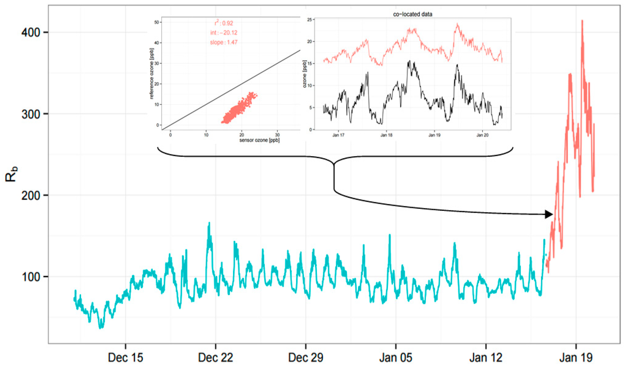
Figure 1 illustrates a sensor that had an increasing and unstable Rb over time. The sensor was returned to the lab and compared against a Model 49i Thermo O3 analyzer where it was observed to record higher values and suppressed diurnal pattern. However, O3 response remained high (R2 = 0.92) and so, following post-calibration, sensor data was salvageable.
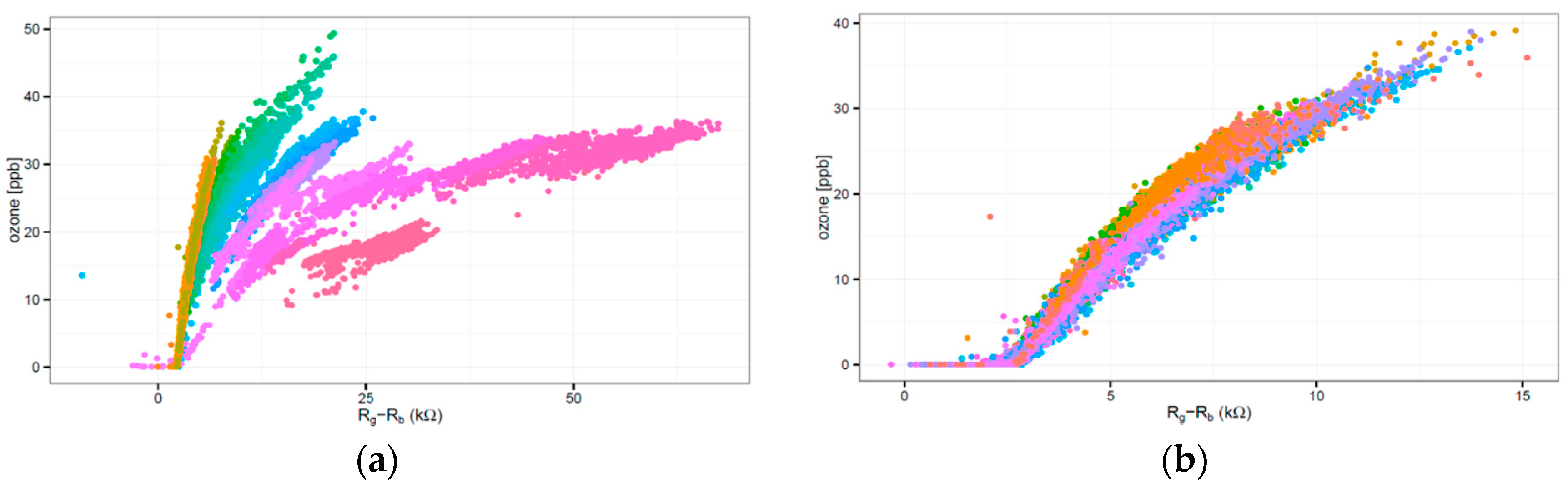
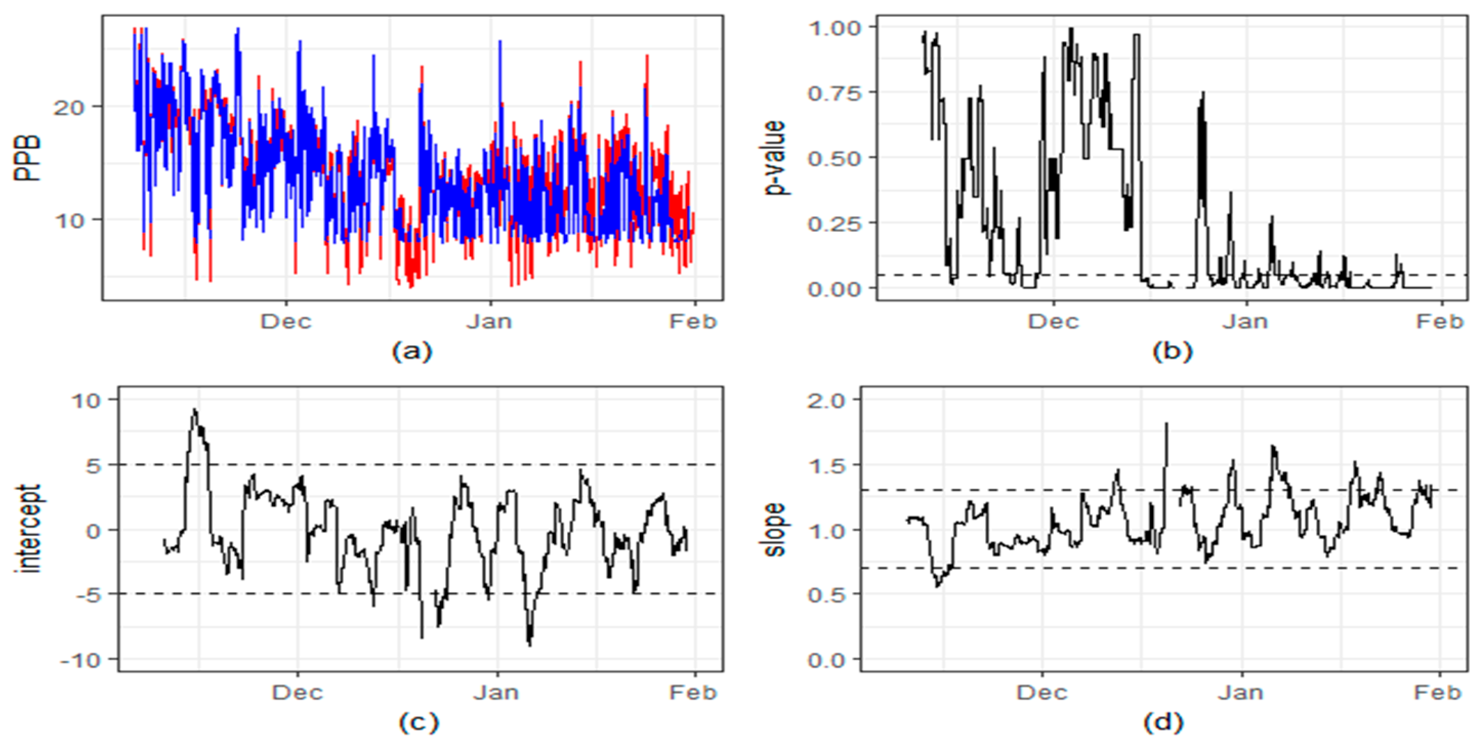
Equation (3) against P successfully detected drifting sensors (Figure 2). The running statistical tests were also successful in identifying sensor drift, with many divergences detected within one-week (Figure 3). The MV test was found to give more robust results due to error thresholds being set by practical limits. The KS test is defined by a probability distribution that relies on concentration range and is prone to statistical significance (which may not be of practical significance). These tests illustrated their use in automated management of network, as daily reporting allowed the network manager to have an objective opinion on the state of each sensor, and optimise time spent on maintenance.
A network of sensors (n = 12) were used to reveal O3 patterns not identified in the regulatory network (n = 3) around Auckland, New Zealand. Examination of instrument siting, where surroundings may affect concentrations, showed good agreement to analyzers within 20 km [10]. No bias was identified between those sensors placed on regulatory stations and those sensors placed upon walls or balconies, giving confidence that both instrument and siting did not affect the reported data. Overall, O3 was low across Auckland, which is believed due to low background concentrations, low long-range transport, and NOX titration. Low concentrations were found for those locations in residential settings, especially during commuting periods and at night [11].
4. Discussion
Low-cost semiconductor sensors were successfully used in a long-term air-quality network, with characterization of calibration drift using data-driven algorithms. This sensor network demonstrated that when operated using automated data quality checks, these sensors could be used in environmental science to provide unique supplementary information to existing regulatory networks.
Acknowledgments
This work was supported by a Callaghan Innovation PhD scholarship for GM (AIRQU1301/34810), a University of Auckland Faculty Research Development Fund (UoA FRDF 3704143), and a Ministry of Business, Innovation, & Employment contract (UOAX1413). We thank Anna Spyker and Shanon Lim, along with other research assistants, along with those individuals who generously hosted devices.
Conflicts of Interest
D.W., G.S. shareholders in Aeroqual Ltd. Funding sponsors had no role in design of the study; in collection, or analysis of data; in writing the manuscript, or in decision to publish results.
References
- Bourgeois, W.; Romain, A.C.; Nicholas, J.; Stuetz, R.M. The use of sensor arrays for environmental monitoring: Interests and limitations. J. Environ. Monit. 2003, 5, 852–860. [Google Scholar] [CrossRef]
- Kumar, P.; Morawska, L.; Martani, C.; Biskos, G.; Neophytou, M.; Di Sabatino, S.; Bell, M.; Norford, L.; Britter, R. The rise of low-cost sensing for managing air pollution in cities. Environ. Int. 2015, 75, 199–205. [Google Scholar] [CrossRef]
- Heimann, I.; Bright, V.B.; McLeod, M.W.; Mead, M.I.; Popoola, O.A.M.; Stewart, G.B.; Jones, R.L. Source attribution of air pollution by spatial scale separation using high spatial density networks of low cost air quality sensors. Atmos. Environ. 2015, 113, 10–19. [Google Scholar] [CrossRef]
- Bart, M.; Williams, D.E.; Ainslie, B.; McKendry, I.; Salmond, J.; Grange, S.K.; Alavi-Shoshtari, M.; Steyn, D.; Henshaw, G.S. High density ozone monitoring using gas sensitive semi-conductor sensors in the Lower Fraser Valley, British Columbia. Environ. Sci. Technol. 2014, 48, 3970–3977. [Google Scholar] [CrossRef] [PubMed]
- Williams, D.E.; Henshaw, G.S.; Bart, M.; Laing, G.; Wagner, J.; Naisbitt, S.; Salmond, J.A. Validation of low-cost ozone measurement instruments suitable for use in an air-quality monitoring network. Meas. Sci. Technol. 2013, 24. [Google Scholar] [CrossRef]
- De Vito, S.; Piga, M.; Martinotto, L.; Di Franca, G. CO, NO2 and NOX urban pollution monitoring with on-field calibrated electronic nose by automatic bayesian regularization. Sens. Actuators B Chem. 2009, 143, 182–191. [Google Scholar] [CrossRef]
- Chabanis, G.; Parkin, I.P.; Williams, D.E. A simple equivalent circuit model to represent microstructure effects on the response of semiconducting oxide-based gas sensors. Meas. Sci. Technol. 2003, 14, 76–86. [Google Scholar] [CrossRef]
- Williams, D.E.; Pratt, K.F. Microstructure effects on the response of gas-sensitive resistors based on semiconducting oxides. Sens. Actuators B Chem. 2000, 70, 214–221. [Google Scholar] [CrossRef]
- Miskell, G.; Salmond, J.A.; Alavi-Shoshtari, M.; Bart, M.; Ainslie, B.; Grange, S.; McKendry, I.G.; Henshaw, G.S.; Williams, D.E. Data verification tools for minimizing management costs of dense air-quality monitoring networks. Environ. Sci. Technol. 2016, 50, 835–846. [Google Scholar] [CrossRef] [PubMed]
- Miskell, G.; Salmond, J.A.; Williams, D.E. Low-cost sensors and crowd-sourced data: Observations of siting impacts on a network of air-quality instruments. Sci. Total Environ. 2017, 575, 1119–1129. [Google Scholar] [CrossRef] [PubMed]
- Weissert, L.F.; Salmond, J.A.; Miskell, G.; Alavi-Shoshtari, M.; Grange, S.K.; Henshaw, G.S.; Williams, D.E. Use of a dense monitoring network of low-cost instruments to observe local changes in the diurnal ozone cycles as marine air passes over a geographically isolated urban center. Sci. Total Environ. 2017, 575, 67–78. [Google Scholar] [CrossRef] [PubMed]
Figure 1.
Sensor baseline (Rb) where it increased (pink). Inset: co-location correlation and time-series to analyzer (black) during the unstable baseline period.
Figure 1.
Sensor baseline (Rb) where it increased (pink). Inset: co-location correlation and time-series to analyzer (black) during the unstable baseline period.

Figure 2.
Sensor gas (Rg)—sensor baseline (Rb) over time (a) Unstable baseline; (b) Stable baseline.
Figure 2.
Sensor gas (Rg)—sensor baseline (Rb) over time (a) Unstable baseline; (b) Stable baseline.

Figure 3.
(a) Co-located sensor measurements; (b) KS-test p-value output; (c) MV-test intercept output; (d) MV-test slope output.
Figure 3.
(a) Co-located sensor measurements; (b) KS-test p-value output; (c) MV-test intercept output; (d) MV-test slope output.

© 2017 by the authors. Licensee MDPI, Basel, Switzerland. This article is an open access article distributed under the terms and conditions of the Creative Commons Attribution (CC BY) license (https://creativecommons.org/licenses/by/4.0/).
Share and Cite
MDPI and ACS Style
Miskell, G.; Salmond, J.; Grange, S.; Weissert, L.; Henshaw, G.; Williams, D. Reliable Long-Term Data from Low-Cost Gas Sensor Networks in the Environment. Proceedings 2017, 1, 400. https://doi.org/10.3390/proceedings1040400
AMA Style
Miskell G, Salmond J, Grange S, Weissert L, Henshaw G, Williams D. Reliable Long-Term Data from Low-Cost Gas Sensor Networks in the Environment. Proceedings. 2017; 1(4):400. https://doi.org/10.3390/proceedings1040400
Chicago/Turabian StyleMiskell, Georgia, Jennifer Salmond, Stuart Grange, Lena Weissert, Geoff Henshaw, and David Williams. 2017. "Reliable Long-Term Data from Low-Cost Gas Sensor Networks in the Environment" Proceedings 1, no. 4: 400. https://doi.org/10.3390/proceedings1040400