Using the Effective Sample Size as the Stopping Criterion in Markov Chain Monte Carlo with the Bayes Module in Mplus

Abstract

Bayesian modeling using Markov chain Monte Carlo (MCMC) estimation requires researchers to decide not only whether estimation has converged but also whether the Bayesian estimates are well-approximated by summary statistics from the chain. On the contrary, software such as the Bayes module in Mplus, which helps researchers check whether convergence has been achieved by comparing the potential scale reduction (PSR) with a prespecified maximum PSR, the size of the MCMC error or, equivalently, the effective sample size (ESS), is not monitored. Zitzmann and Hecht (2019) proposed a method that can be used to check whether a minimum ESS has been reached in Mplus. In this article, we evaluated this method with a computer simulation. Specifically, we fit a multilevel structural equation model to a large number of simulated data sets and compared different prespecified minimum ESS values with the actual (empirical) ESS values. The empirical values were approximately equal to or larger than the prespecified minimum ones, thus indicating the validity of the method.

1. Introduction

Bayesian modeling has gained popularity in psychology [1] and related sciences [2] because Bayesian modeling can be beneficial in several respects; for example, it offers greater flexibility in modeling (e.g., [3]), fewer estimation problems (e.g., [4]), and more accurate estimates, (e.g., [5]), particularly when models with latent variables are estimated. Most software uses Markov chain Monte Carlo (MCMC) methods, which generate samples from the distribution of the population parameters given the data (i.e., the posterior distribution). However, Bayesian modeling requires researchers not only to decide which prior distributions they want to use, a task that is often challenging for researchers (e.g., [6]), but also to judge whether estimation has converged and whether the Bayesian estimates are approximated reasonably well by summary statistics from the MCMC chain. To ensure a high level of precision, the MCMC error needs to be small (e.g., [7]). Software such as the Bayes module in Mplus [8] routinely monitors convergence by checking whether a certain value for the potential scale reduction (PSR; [9]) has been reached. This value can be specified by the user, whereas a value for the amount of the MCMC error or, equivalently, for the effective sample size (ESS), cannot be specified directly. However, Zitzmann and Hecht [10] proposed a method that can be used to control the ESS in Mplus, taking advantage of a correspondence between the ESS and the PSR, which exists when both coefficients are computed with the help of estimates from the analysis of variance (ANOVA) literature that are based on the mean squares. By “control”, we mean that users can specify a minimum ESS and thus a minimum level of precision as the stopping criterion before the estimation is carried out.

Because this method was only proposed but not evaluated by the authors, the goal of the present article is to evaluate the method with a computer simulation. Specifically, we simulated and analyzed about a thousand data sets from a simple multilevel structural equation model that is often applied in organizational and educational research, and we compared different prespecified minimum values of the ESS with the actual empirically obtained values of the ESS.

2. Zitzmann and Hecht’s Method

Various criteria for monitoring convergence have been suggested in the literature, most notably the PSR. We consider a single long run of the MCMC sampler, see [7,11]. Then, the PSR for a parameter $\theta$ is defined by Gelman and Rubin [9] as:

$$\mathrm{PSR}=\sqrt{{\widehat{\sigma }}_{\theta }^2/W}$$

(1)

where ${\widehat{\sigma }}_{\theta }^2$ is the variance of the MCMC chain for $\theta$ and is given by an estimate from the ANOVA literature: ${\widehat{\sigma }}_{\theta }^2=\left(L-1\right)W/L+B/L$. $W={\sum }_{j=1}^m\left[{\sum }_{i=1}^L{\left({\theta }_{ij}-{\overline{\theta }}_{•j}\right)}^2/\left(L-1\right)\right]/m$ is the average of the variances within equally long, nonoverlapping sequences of the chain, where m is the number of sequences, and L is the length of the sequences. $B/L={\sum }_{j=1}^m{\left({\overline{\theta }}_{•j}-{\overline{\theta }}_{••}\right)}^2/\left(m-1\right)$ is the variance between sequences ([3,9]). Mplus uses the PSR in the following algorithm, which automatically determines when to stop the estimation:

• Generate iterative samples for each parameter, which constitute one MCMC chain per parameter.
• After every 100th iteration, discard the first half of each chain as burn-in.
• Compute the PSR for each parameter by using the remaining samples. When the PSR values of all parameters fall below the prespecified maximum PSR value, then stop. Otherwise, continue with the estimation. The maximum PSR value can be set manually, and we will make use of this feature later on.

The PSR is meant to assess convergence. However, it has been argued that besides convergence, another condition must be met before Bayesian estimates are computed. The number of independent samples from the posterior distribution (i.e., the Effective Sample Size; ESS) must be large to guarantee precise approximations of the estimates (e.g., [7,10,11]). Therefore, it is generally recommended that the ESS should also be monitored. One possible way of doing this is by adapting Mplus’ stopping algorithm to check for convergence. The adapted algorithm proceeds as follows:

• Run an MCMC chain for each parameter.
• After every 100th iteration, discard the first half of each chain (burn-in phase).
• Compute the ESS for each parameter from the remaining samples. When all ESS values lie above the prespecified minimum ESS value, stop the estimation. Otherwise, continue with it. It is interesting to note that because of the correspondence between the ESS and the PSR, this algorithm also ensures that all PSR values will fall below a certain “implied” maximum PSR value and, thus, that convergence will generally also be reached.

Mplus provides the algorithm for monitoring the convergence of the chain and an option to specify the maximum value for the PSR as the stopping criterion, whereas Mplus does not provide such an algorithm for the ESS. This led Zitzmann and Hecht [10] to suggest a simple solution.

Linking the PSR and the ESS

The basic idea behind the method is the observation that there is a link between the ESS and the PSR, which becomes apparent when the estimators from the ANOVA literature used by Gelman and Rubin [9] in their PSR coefficient are also used in the computation of the ESS. For a parameter $\theta$, the ESS can be defined as:

$$\mathrm{ESS}={\widehat{\sigma }}_{\theta }^2/\widehat{\mathrm{V}}\left({\overline{\theta }}_{•}\right)$$

(2)

where ${\widehat{\sigma }}_{\theta }^2$ is the variance of the MCMC chain (see above), and $\widehat{\mathrm{V}}\left({\overline{\theta }}_{•}\right)$ is the variance of the chain mean. $\widehat{\mathrm{V}}\left({\overline{\theta }}_{•}\right)$ can be computed as an estimate from the ANOVA literature: $\widehat{\mathrm{V}}\left({\overline{\theta }}_{•}\right)=\left(B/L\right)/m$, where $B/L={\sum }_{j=1}^m{\left({\overline{\theta }}_{•j}-{\overline{\theta }}_{••}\right)}^2/\left(m-1\right)$ is the variance between sequences, L is the sequence length, and m is the number of sequences. This formula was also used by Gelman and Rubin [9]. It is important to note that similar to the PSR, the ESS in Equation (2) is estimated by using estimators from the ANOVA literature. This approach is also used by some software (e.g., in the batch standard error of the R package coda; [12]). However, there are other ways of computing the ESS that are more common in the time-series literature [7]. We will come back to this point later in the article.

To understand how the ESS is related to the PSR, insight can be gained by first rearranging Equation (2) in such a way that only ${\widehat{\sigma }}_{\theta }^2$ is left on the right-hand side and by subsequently inserting this expression into Equation (1). Finally, simplifying the equation yields an expression of the PSR in terms of the ESS. An approximation is given by:

$$\mathrm{PSR}\approx \sqrt{\mathrm{ESS}/\left(\mathrm{ESS}-m\right)}$$

(3)

where m is the number of chain sequences. For details on the derivation, we refer readers to Zitzmann and Hecht [10]. The equation shows that the PSR value decreases when the ESS increases and that the PSR value increases when the number of sequences increases as well.

Equation (3) is the key to implementing the ESS stopping criterion in Mplus. The minimum ESS needs to be chosen first. Because Mplus uses only the third and fourth quarters of the chain (p. 634, [8]), m must be set to 2 (i.e., two chain sequences). Inserting the value for the minimum ESS and the number of sequences into Equation (3) then yields an upper bound for the PSR because the ESS values that are larger than the minimum ESS can only result in PSR values that are smaller than the obtained one. This means that the obtained value for the PSR can be used as the maximum PSR in Mplus.

Unless otherwise specified, Mplus determines the maximum value for the PSR in an automatic fashion by calculating: $\mathrm{PSR}=1+a·0.05$. The a factor depends on the number of model parameters and can take on values between 1 when there is only one parameter and 2 when there are many parameters (p. 634, [8]). In order to specify the maximum PSR obtained from Equation (3) manually, the BCONVERGENCE option must be set equal to $\left(\max .\mathrm{PSR}-1\right)/a$. Because most substantive models include many parameters, it is reasonable to set a to 2. With this setting, Mplus stops only after the prespecified minimum ESS value has been reached.

Although Zitzmann and Hecht [10] suggested this method, it has yet to be evaluated. Therefore, we conducted a computer simulation whose findings are the subject of the next section.

3. Simulation Study

The study was designed to evaluate Zitzmann and Hecht’s solution for using the ESS as the stopping criterion in Mplus. To this end, we simulated data from a multilevel structural equation model and analyzed them with the Bayes module in Mplus, using the proposed method.

3.1. Method

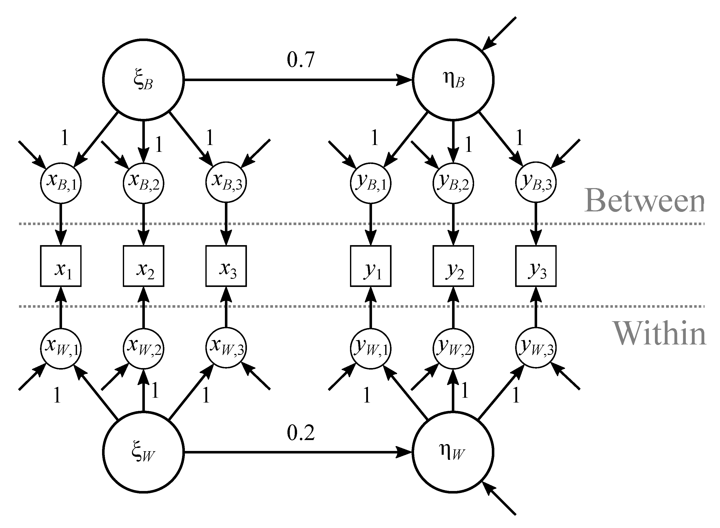
The data-generating model was the multilevel structural equation model in Figure 1. One latent predictor variable predicted a latent dependent variable. Both variables were measured with three indicators, each normally distributed and with a standardized between-group loading of $0.6$ (e.g., [13]). The unstandardized loadings all had values of 1 because the ones from the first indicators were set equal to 1, and the indicators were assumed to be parallel. The (unstandardized) within-group regression coefficient was set equal to $0.2$, and the (unstandardized) between-group regression coefficient was $0.7$. It was further assumed that the intraclass correlations (ICCs; i.e., the proportions of the total variances that were located between groups; [14]) of the dependent variable and the predictor were $0.3$, as were the ICCs of the indicators of these variables. The $0.3$ value falls within the typical range from $0.0$ to $0.4$ [14,15]. The within- and between-group $R^2$s were $0.04$ and $0.49$, respectively. All indicators had a within-group error variance of $1.24$ and a between-group error variance of $0.53$.

Each generated data set consisted of 1000 individuals, who were grouped into 100 groups (10 individuals each). Such a sample size is frequently encountered in multilevel research [16]. We generated 5000 data sets and then analyzed each of them with the Bayes module in Mplus 7.1.

To implement the analysis model in Mplus, we specified a multilevel structural equation model with congeneric indicators with cross-level invariant loadings. To this end, we fixed the within-group loading of the first indicators to 1 to identify the metric of the latent predictor, and we allowed the remaining loadings to be estimated under the constraint that they are equal across the levels (i.e., cross-level invariance). Such constrained models are often applied in research practice because one would not expect loadings to be different across the levels; for example, when configural models are fit (see [17], for a discussion). Notice that the analysis model was slightly more general than the data-generating one (because the analysis model assumed congeneric indicators, whereas the data-generating model assumed only parallel indicators). Thus, although the analysis model did not provide an exact match with the data-generating model, the analysis model covered the data-generating model. Therefore, the results (e.g., biased point estimates) could not be attributed to model misspecification.

To estimate the analysis model with the Bayes module, prior distributions needed to be specified. We adopted the specification from (e.g., Zitzmann et al. [18]) rather than Mplus’ default (see [19], for the argument that software defaults can bias results). More specifically, we specified uninformative normal priors with means of 0 and variances of 1000 for the within- and between-group intercepts, loadings, and slope parameters in the model, and we specified uninformative inverse gamma priors with shape and scale parameters of $0.001$ for the within-group variances and weakly informative inverse gamma priors with shape and scale parameters of $0.1$ for the between-group variances (see also [4]).

In order to evaluate Zitzmann and Hecht’s method, we specified different minimum values for the ESS as stopping criteria (i.e., 25, 50, 100, 200, 300, 400, 500, and 1000 samples), and we computed implied values for the PSR from them with the help of Equation (3), which were set as stopping criteria via the BCONVERGENCE option in Mplus (see the Appendix A for the program code).

We compared each of these prespecified minimum ESS values with the actual (empirical) ESS values from the MCMC chains. We computed the empirical ESS from Equation (2). This way of computing the ESS uses estimators from the ANOVA literature, and it is also used in the proposed method. We will refer to this ESS simply as the “ESS”. In order to be able to compare this way of computing the ESS with other ways of doing so, we additionally computed it by using an alternative estimate of the variance of the chain mean, which is given by: $\widehat{\mathrm{V}}\left({\overline{\theta }}_{•}\right)=\widehat{\lambda }/L_{\mathrm{total}}$, where $\widehat{\lambda }$ is the spectral density of the chain at frequency zero, and $L_{\mathrm{total}}$ is the total length of the chain ([12,20]). This ESS is often used in the time-series literature. We will therefore refer to it as the “time-series ESS”. The third way of computing the ESS involves computing it from the batch standard error, which uses a sufficiently large number of nonoverlapping sequences of the chain (i.e., “batches”). We used 5, 10, and 25 batches. We will refer to this ESS as the “batch ESS”. We expected the empirical ESS values (estimated by the three methods) to be at least as large if not larger than the prespecified minimum ESS values, which would validate the proposed method.

In addition, we compared the different prespecified minimum ESS values with respect to three statistical properties—relative bias, relative root mean squared error (RMSE), and coverage rate—to replicate the findings from Zitzmann and Hecht [10], who demonstrated that the quality of estimates can be suboptimal when the precision with which the Bayesian estimates are approximated is too low because the ESS is too small. For details on how the statistical properties were computed, we refer readers to Lüdtke et al. [21], Muthén and Muthén [22], or Zitzmann and Helm [23].

Before we present the results, it is important to mention that for each data set and analysis, we identified the parameter for which convergence was slowest or, equivalently, for which the empirical ESS as computed by the first method (i.e., by using estimators from the ANOVA literature) was smallest. We used this empirical ESS value along with the ESS values from the other methods in comparison with the prespecified minimum ESS value. We used the point estimate (mean) and interval estimate of the parameter ($2.5$th and $97.5$th percentiles) to compute the relative bias, relative RMSE, and coverage rate.

3.2. Results

We focused on the following parameters of the between-model in Figure 1: the regression coefficient, which is often the most interesting parameter, the variance of the predictor, and the residual variance. We begin with an inspection of the correspondence between the empirical and the prespecified minimum ESS, followed by an inspection of how the statistical properties vary depending on the prespecified minimum ESS.

3.2.1. Comparison between the Prespecified ESS and the Empirical ESS

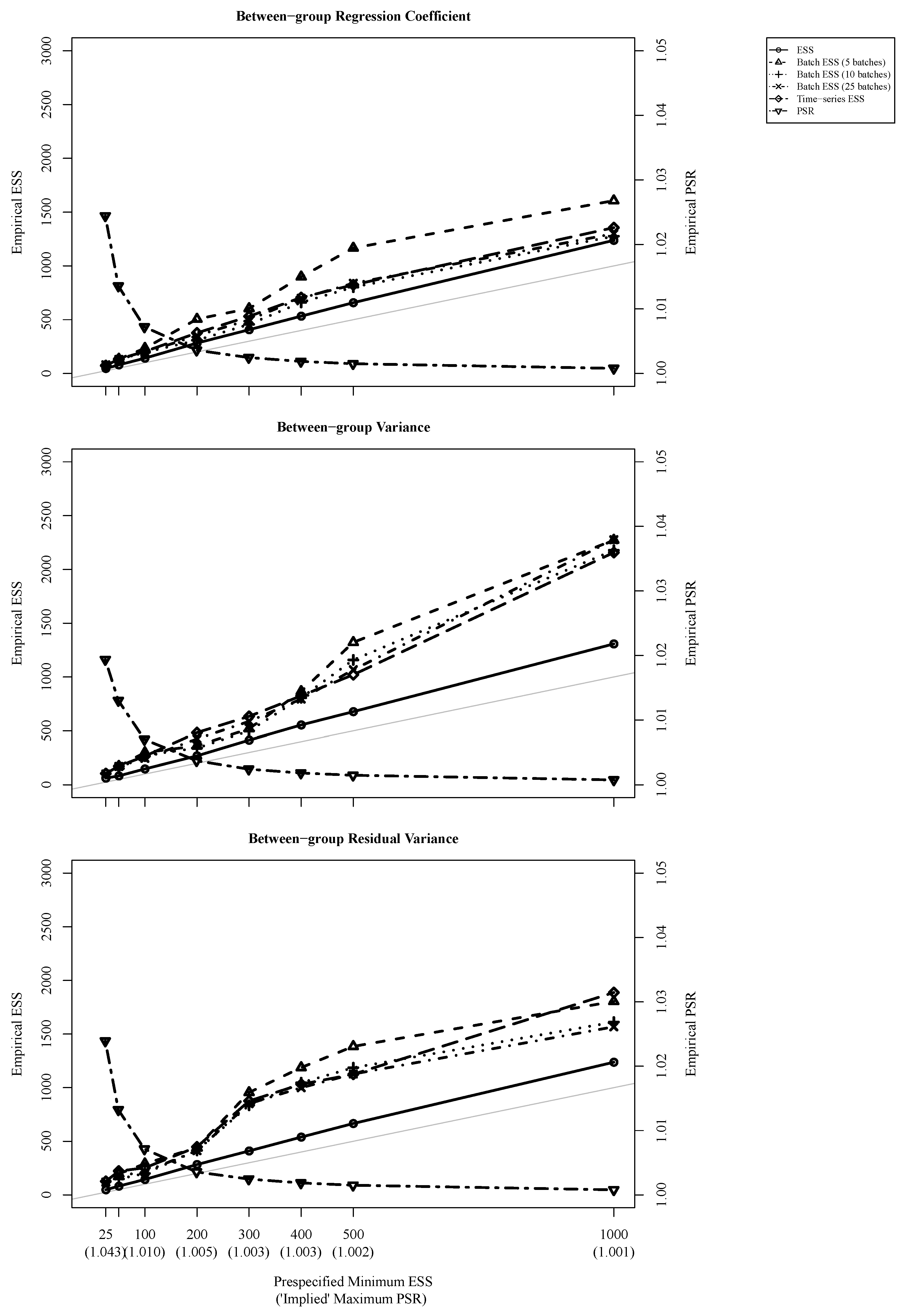
To facilitate the comparison, we created a series of plots that visually represent the results for the three parameters. The plots can be found in Figure 2. They show the average empirical ESS values (averaged across data sets) for the different prespecified minimum ESS values. We added bisectors to the plots (grey lines) because they help assess how much the prespecified minimum ESS and the empirical ESS differed. Points that are close to a bisector indicate that the empirical ESS was close to the prespecified minimum ESS. Points situated above the bisector indicate that the empirical ESS was larger than the prespecified minimum ESS, and points below the bisector indicate that the empirical ESS was smaller than the prespecified minimum ESS. Furthermore, we added the implied maximum PSR and the empirical PSR.

A first look at Figure 2 reveals that most of the points were situated above the bisectors, indicating that the empirical ESS values were larger than the prespecified minimum ESS values. In particular, this also means that the empirical values were not smaller than the prespecified minimum ones. Because the method is aimed at ensuring that the empirical ESS values will be at least as large as the prespecified ESS values, this finding speaks for the validity of the method. The empirical ESS values were closest to the prespecified minimum ESS values in the low ESS range and they deviated more from the prespecified minimum ESS values in the upper ESS range. Moreover, there was a tendency for the three different methods that we used to compute the ESS to yield different results. More specifically, the method that uses estimates from the ANOVA literature (denoted as “ESS” in the figure) yielded the smallest ESS values, which were very close to the prespecified minimum ESS values. This is not very surprising and could have been expected because the proposed method is based on this way of computing the ESS. The different specifications of the batch ESS provided different results, with the batch ESS with 25 batches providing results similar to the time-series ESS. In addition to this overall validation, the figure shows that a larger ESS value was associated with a smaller PSR value.

3.2.2. Statistical Properties

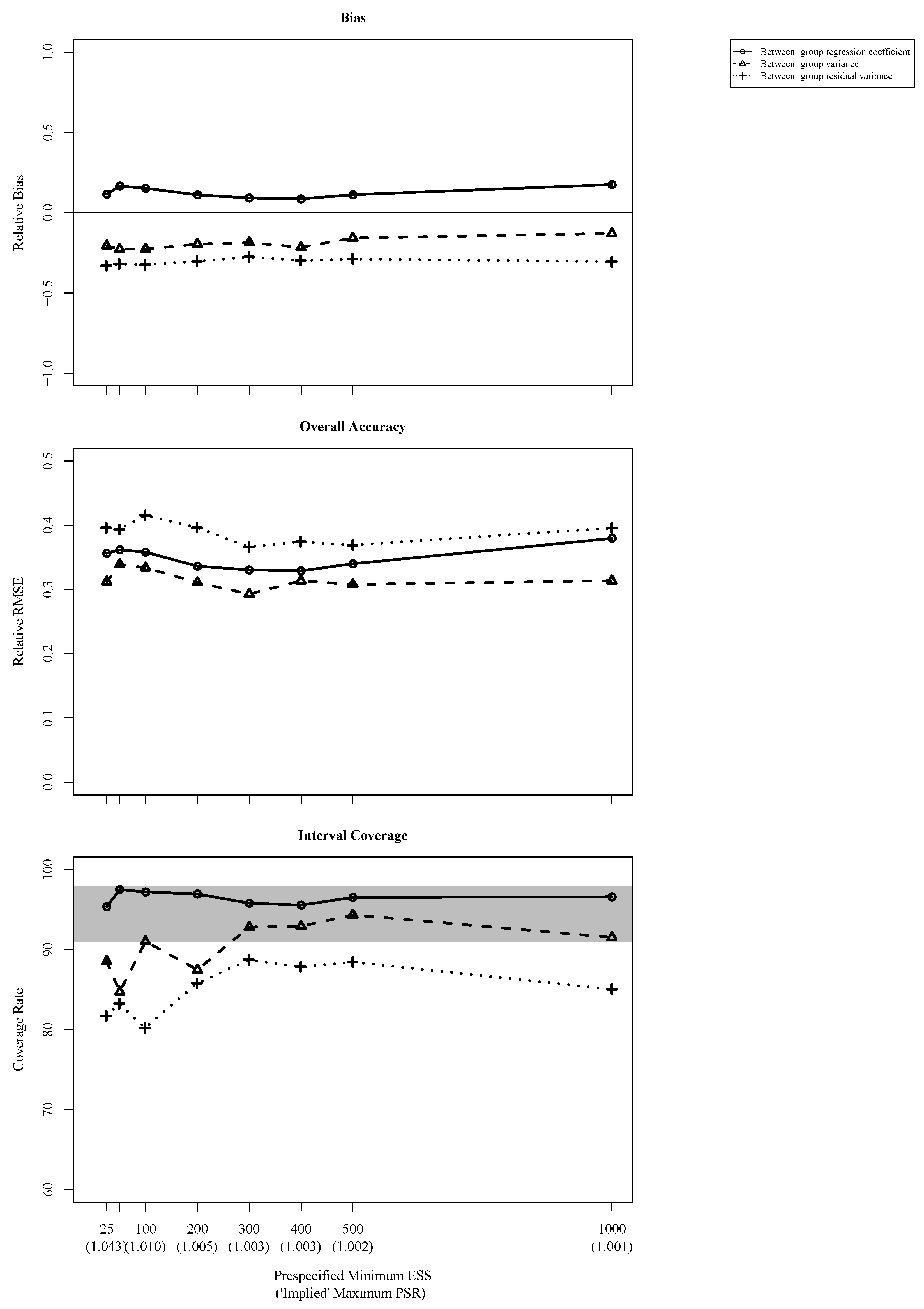
Figure 3 shows a series of plots that compare the statistical properties of the different prespecified minimum ESS values. Although the analysis model covered the data-generating model, the MCMC method provided substantially biased estimates of the three parameters from the between-model (i.e., they exhibited relative biases of more than $\pm 0.1$). The estimates of the regression coefficient were positively biased, whereas the estimates of the variance of the predictor and the residual variance were both negatively biased. However, given that samples of 100 groups with 10 individuals each are rather small, and given that the estimates will be unbiased only when samples are large, these biases could have been expected.

The estimates were least accurate (i.e., they exhibited the largest relative RMSEs) when the prespecified minimum ESS was small (i.e., <400) but tended to become more accurate when the prespecified minimum ESS increased up to a large value (i.e., 1000).

A similar picture emerged with regard to the coverage rate. Some of the coverage rates were unacceptably low (i.e., <91%) with a small prespecified minimum ESS, particularly those of the variance estimates. However, they tended to become acceptable when the prespecified minimum ESS increased, thus supporting Zitzmann and Hecht’s (2019) claim that the ESS must be large enough to guarantee good statistical properties.

4. Discussion

Many researchers who employ latent variable modeling fit these models with Mplus. There might be multiple reasons for this practice. Mplus is specifically written for latent variable models. Moreover, models can be specified very easily, and the Bayes module in Mplus seems to be very efficient [18]. However, although Mplus monitors convergence by routinely checking the PSR, it does not monitor the ESS. Therefore, Zitzmann and Hecht [10] proposed a method that can be used to control the ESS in Mplus. This article validated the proposed method with the help of a computer simulation. The main findings can be summarized as follows. First and foremost, our results showed that the empirical ESS values were larger but not smaller than the prespecified minimum ESS values, indicating the validity of the method. It is interesting that the different methods for computing the ESS tended to yield different results—which deserves some attention. Only recently, Vehtari et al. [24] proposed another way of computing the ESS, which might be more trustworthy than the other methods. However, empirical support for this speculation is lacking so far. Moreover, the results showed that the statistical properties of the point and interval estimates were suboptimal when the ESS was too small, which demonstrated once more the importance of specifying software in such a way that the ESS will be large and, thus, that the precision with which the Bayesian estimates are approximated is sufficiently high [10]. Fewer than 400 samples are generally not recommended, and 1000 samples are optimal [10]. Note that, overall, the autocorrelation was relatively high (>0.8), indicating that the ESS was much smaller than the number of iterations. More informative priors will likely result in a lower autocorrelation and thus a larger ESS per second (ESS/s), reducing the time needed to achieve an ESS that is large enough [25].

The stopping algorithm for checking the ESS can also be implemented in other software. For example, Hecht et al. ([26]; see also [27]) implemented a very similar algorithm for JAGS [12], which also uses MCMC but is freely available. The algorithm is automated, meaning that the algorithm automatically decides when to stop. This may be an improvement for many researchers. A detailed description of the algorithm can be found in Hecht et al.’s article. For the program code, see their Supplemental Material. However, it should be noted that the authors used the ESS from Shinystan [28], which differs from ours.

In future research, it would be interesting to also investigate the solution in situations in which convergence and precise approximations will be difficult to achieve with MCMC methods when the abovementioned prior distributions are adopted (e.g., inverse gamma priors with shapes and scales of $0.1$ for between-group error variances). Such a situation will likely arise when shared-and-configural models are estimated and strong factorial invariance holds across higher level units; that is, the between-group error variances are equal to zero, see [29]. The shared-and-configural model was proposed by Stapleton et al. [17] as a way to separate the “objective” shared factor from a nuisance factor. Because inverse gamma priors with shapes and scales larger than $0.001$ (a) do not allow variance estimates that are negative, (b) avoid estimates that are close to zero, and (c) give particular weight to variances that are substantial (e.g., [30,31]), the sampler will struggle in this case. Furthermore, it would be interesting to compare Vehtari et al.’s method for computing the ESS with other existing methods by means of extensive simulation in order to verify whether their method can outperform the other methods.

Most of the software that provides Bayesian modeling uses MCMC methods. However, the application of these methods is not without its challenges. We discussed one such challenge here and validated a solution to this challenge. We hope that our findings will provide confidence in the method and that the article will contribute to the use of software such as Mplus in an informed way.

References

- van de Schoot, R.; Winter, S.D.; Ryan, O.; Zondervan-Zwijnenburg, M.; Depaoli, S. A systematic review of Bayesian articles in psychology: The last 25 years. Psychol. Methods 2017, 22, 217–239. [Google Scholar] [CrossRef]
- König, C.; van de Schoot, R. Bayesian statistics in educational research: A look at the current state of affairs. Educ. Rev. 2018, 70, 486–509. [Google Scholar] [CrossRef]
- Muthén, B.O.; Asparouhov, T. Bayesian structural equation modeling: A more flexible representation of substantive theory. Psychol. Methods 2012, 17, 313–335. [Google Scholar] [CrossRef] [PubMed]
- Depaoli, S.; Clifton, J.P. A Bayesian approach to multilevel structural equation modeling With continuous and dichotomous outcomes. Struct. Equ. Model. 2015, 22, 327–351. [Google Scholar] [CrossRef]
- Zitzmann, S.; Lüdtke, O.; Robitzsch, A.; Hecht, M. On the performance of Bayesian approaches in small samples: A comment on Smid, McNeish, Miočević, and van de Schoot (2020). STructural Equ. Model. 2021, 28, 40–50. [Google Scholar] [CrossRef]
- Gelman, A. Prior distributions for variance parameters in hierarchical models (comment on article by Browne and Draper). Bayesian Anal. 2006, 1, 515–534. [Google Scholar] [CrossRef]
- Geyer, C.J. Practical Markov chain Monte Carlo. Stat. Sci. 1992, 7, 473–511. [Google Scholar] [CrossRef]
- Muthén, L.K.; Muthén, B.O. Mplus User’s Guide, 7th ed.; Muthén & Muthén: Los Angeles, CA, USA, 2012. [Google Scholar]
- Gelman, A.; Rubin, D.B. Inference from iterative simulation using multiple sequences. Stat. Sci. 1992, 7, 457–472. [Google Scholar] [CrossRef]
- Zitzmann, S.; Hecht, M. Going beyond convergence in Bayesian estimation: Why precision matters too and how to assess it. Struct. Equ. Model. 2019, 26, 646–661. [Google Scholar] [CrossRef]
- Link, W.A.; Eaton, M.J. On thinning of chains in MCMC. Methods Ecol. Evol. 2012, 3, 112–115. [Google Scholar] [CrossRef]
- Plummer, M.; Best, N.; Cowles, K.; Vines, K.; Sarkar, D.; Bates, D.; Almond, R.; Magnusson, A. Package ‘Coda’ [Computer Software Manual]. 2016. Available online: https://cran.r-project.org/web/packages/coda/coda.pdf (accessed on 20 July 2021).
- Lüdtke, O.; Marsh, H.W.; Robitzsch, A.; Trautwein, U. A 2 × 2 taxonomy of multilevel latent contextual models: Accuracy-bias trade-offs in full and partial error correction models. Psychol. Methods 2011, 16, 444–467. [Google Scholar] [CrossRef]
- Snijders, T.A.B.; Bosker, R.J. Multilevel Analysis: An Introduction to Basic and Advanced Multilevel Modeling, 2nd ed.; Sage: Los Angeles, CA, USA, 2012. [Google Scholar]
- Gulliford, M.C.; Ukoumunne, O.C.; Chinn, S. Components of variance and intraclass correlations for the design of community-based surveys and intervention studies: Data from the Health Survey for England 1994. Am. J. Epidemiol. 1999, 149, 876–883. [Google Scholar] [CrossRef]
- Hox, J.J.; Maas, C.J.M.; Brinkhuis, M.J.S. The effect of estimation method and sample size in multilevel structural equation modeling. Stat. Neerl. 2010, 64, 157–170. [Google Scholar] [CrossRef]
- Stapleton, L.M.; Yang, J.S.; Hancock, G.R. Construct meaning in multilevel settings. J. Educ. Behav. Stat. 2016, 41, 481–520. [Google Scholar] [CrossRef]
- Zitzmann, S.; Lüdtke, O.; Robitzsch, A.; Marsh, H.W. A Bayesian approach for estimating multilevel latent contextual models. Struct. Equ. Model. 2016, 23, 661–679. [Google Scholar] [CrossRef]
- Smid, S.C.; Winter, S.D. Dangers of the defaults: A tutorial on the impact of default priors when using Bayesian SEM with small samples. Front. Psychol. 2020, 11, 3536. [Google Scholar] [CrossRef]
- Jackman, S. Bayesian Analysis for the Social Sciences; Wiley: Chichester, UK, 2009. [Google Scholar]
- Lüdtke, O.; Marsh, H.W.; Robitzsch, A.; Trautwein, U.; Asparouhov, T.; Muthén, B.O. The multilevel latent covariate model: A new, more reliable approach to group-level effects in contextual studies. Psychol. Methods 2008, 13, 203–229. [Google Scholar] [CrossRef] [Green Version]
- Muthén, L.K.; Muthén, B.O. How to use a Monte Carlo study to decide on sample size and determine power. Struct. Equ. Model. 2002, 9, 599–620. [Google Scholar] [CrossRef]
- Zitzmann, S.; Helm, C. Multilevel analysis of mediation, moderation, and nonlinear effects in small samples, using expected a posteriori estimates of factor scores. Struct. Equ. Model. 2021, 28, 529–546. [Google Scholar] [CrossRef]
- Vehtari, A.; Gelman, A.; Simpson, D.; Carpenter, B.; Bürkner, P.C. Rank-normalization, folding, and localization: An improved for assessing convergence of MCMC. Bayesian Anal. 2021. [Google Scholar] [CrossRef]
- Hecht, M.; Weirich, S.; Zitzmann, S. Comparing the Effective Sample Size Performance of JAGS and Stan. 2021; submitted. [Google Scholar]
- Hecht, M.; Gische, C.; Vogel, D.; Zitzmann, S. Integrating out nuisance parameters for computationally more efficient Bayesian estimation—An illustration and tutorial. Struct. Equ. Model. 2020, 27, 483–493. [Google Scholar] [CrossRef]
- Hecht, M.; Zitzmann, S. A computationally more efficient Bayesian approach for estimating continuous-time models. Struct. Equ. Model. 2020, 27, 829–840. [Google Scholar] [CrossRef]
- Gabry, J. Shinystan: Interactive Visual and Numerical Diagnostics and Posterior Analysis for Bayesian Models [Computer Software Manual]. 2016. Available online: http://cran.r-project.org/package=shinystan (accessed on 20 July 2021).
- Jak, S.; Jorgensen, T.D.; Rosseel, Y. Evaluating cluster-level factor models with lavaan and Mplus. Psych 2021, 3, 134–152. [Google Scholar] [CrossRef]
- Zitzmann, S.; Lüdtke, O.; Robitzsch, A. A Bayesian approach to more stable estimates of group-level effects in contextual studies. Multivar. Behav. Res. 2015, 50, 688–705. [Google Scholar] [CrossRef]
- Chung, Y.; Rabe-Hesketh, S.; Dorie, V.; Gelman, A.; Liu, J. A nondegenerate penalized likelihood estimator for variance parameters in multilevel models. Psychometrika 2013, 78, 685–709. [Google Scholar] [CrossRef] [Green Version]
Figure 1.
Data-generating model.
Figure 2.
Empirically obtained effective sample size (ESS) and the empirically obtained potential scale reduction (PSR) as a function of the prespecified minimum effective sample size. The grey lines are the bisectors, indicating the identities of the prespecified minimum ESS and the empirical ESS.
Figure 3.
Relative bias, relative root mean squared error (RMSE), and coverage rate for the different prespecified minimum effective sample sizes.
Publisher’s Note: MDPI stays neutral with regard to jurisdictional claims in published maps and institutional affiliations. |
© 2021 by the authors. Licensee MDPI, Basel, Switzerland. This article is an open access article distributed under the terms and conditions of the Creative Commons Attribution (CC BY) license (https://creativecommons.org/licenses/by/4.0/).
Share and Cite
MDPI and ACS Style
Zitzmann, S.; Weirich, S.; Hecht, M. Using the Effective Sample Size as the Stopping Criterion in Markov Chain Monte Carlo with the Bayes Module in Mplus. Psych 2021, 3, 336-347. https://doi.org/10.3390/psych3030025
AMA Style
Zitzmann S, Weirich S, Hecht M. Using the Effective Sample Size as the Stopping Criterion in Markov Chain Monte Carlo with the Bayes Module in Mplus. Psych. 2021; 3(3):336-347. https://doi.org/10.3390/psych3030025
Chicago/Turabian StyleZitzmann, Steffen, Sebastian Weirich, and Martin Hecht. 2021. "Using the Effective Sample Size as the Stopping Criterion in Markov Chain Monte Carlo with the Bayes Module in Mplus" Psych 3, no. 3: 336-347. https://doi.org/10.3390/psych3030025