Portfolio Optimization under Correlation Constraint


1
Bank of America Securities, New York, NY 10036, USA
2
Department of Mathematics and Statistics, McMaster University, 1280 Main Street West, Hamilton, ON L8S 4K1, Canada
*
Author to whom correspondence should be addressed.
Risks 2020, 8(1), 15; https://doi.org/10.3390/risks8010015
Submission received: 29 December 2019
/
Revised: 25 January 2020
/
Accepted: 3 February 2020
/
Published: 6 February 2020
(This article belongs to the Special Issue Systemic Risk in Finance and Insurance)
Abstract
:We consider the problem of portfolio optimization with a correlation constraint. The framework is the multi-period stochastic financial market setting with one tradable stock, stochastic income, and a non-tradable index. The correlation constraint is imposed on the portfolio and the non-tradable index at some benchmark time horizon. The goal is to maximize a portofolio’s expected exponential utility subject to the correlation constraint. Two types of optimal portfolio strategies are considered: the subgame perfect and the precommitment ones. We find analytical expressions for the constrained subgame perfect (CSGP) and the constrained precommitment (CPC) portfolio strategies. Both these portfolio strategies yield significantly lower risk when compared to the unconstrained setting, at the cost of a small utility loss. The performance of the CSGP and CPC portfolio strategies is similar.
1. Introduction
Mean variance optimization introduced by Markowitz (1952) changed the pathway of how fund managers look at optimal investments. However, mean variance analysis is a special case of more general expected utility framework introduced by von Neumann and Morgenstern (1947). Our goal is to maximize expected exponential utility function subject to a correlation constraint. Portfolio optimization under correlation constraints is of particular interest to hedge funds which implement market defensive strategies with higher returns during down markets than up-markets, and this makes our research interesting from a practical standpoint.
Although portfolio allocation within expected utility paradigm is very well explored problem in finance, few studies have considered portfolio allocation with correlation constraint. Recent works that stand out and are also the motivation of this study are Bernard and Vanduffel (2014), Pourbabaee et al. (2016), Bernard et al. (2018), Kondor et al. (2017), and Landsman et al. (2018). In Bernard and Vanduffel (2014), the authors addressed the problem of mean variance optimization along with correlations constraint. The work Pourbabaee et al. (2016) looks at the problem of capital allocation with correlation constraint, and the objective is minimizing capital at risk. The paper Bernard et al. (2018) extended Bernard and Vanduffel (2014), and Pourbabaee et al. (2016) to law invariant preferences. The work Kondor et al. (2017) provides analytic solutions to variance minimization problem with no short-selling constraint. The paper Landsman et al. (2018) finds explicit solutions for optimizing a generalized measure applied to constrained and unconstrained portfolios. All these works consider a static framework; the optimization is performed at time zero and the optimal strategies are implemented. However, if at a later time the optimization criterion and the risk constraint are dynamically updated the time zero strategy fails to remain optimal due to the correlation constraint; this is referred to as time inconsistency. In the presence of a commitment mechanism the time zero optimal strategy, also known as the precommitment strategy, will be implemented. Otherwise, there will be an incentive to deviate from the precommitment strategy and one way out of this predicament is to consider the subgame perfect strategy, also known as the Nash equilibrium strategy.
This paper considers the expected exponential utility maximization with correlation constraint in a discrete time setting. The multi-period stochastic financial market comprises one tradable stock, stochastic income, and a non-tradable index. The non-linearity of correlation constraint turn the optimization problem time inconsistent as explained above. The constrained subgame perfect strategy (CSGP) is naturally defined in our context through backward induction. The constrained precommitment strategy (CPC) is considered as well. We compare the performance of these two portfolio strategies against the unconstrained subgame perfect strategy (UnSGP).
Contribution: Our first and foremost contribution is the analytic solutions for the CSGP and CPC strategies. To the best of our knowledge, we are not aware of other studies that consider time inconsistency arising due to the correlation constraint in the context of portfolio optimization in a multi-period setting. Secondly, through numerical simulations we provide evidence for significant risk reduction in a “high risk” environment by following CSGP and CPC strategies compared to the UnSGP strategy. To illustrate an example, the increase in uncertainty due to increasing the investment horizon from 2 period to 10 period results in a 50% improvement in utility at the expense of a 150% increase in risk for the UnSGP strategy. In contrast, our CSGP strategy results in 30% improvement in utility together with 18% reduction in risk. Thirdly, we find the CSGP and CPC strategy to perform approximately the same for our portfolio allocation problem. This in contrast to the results in Wu (2013) where authors find the CPC strategy to significantly outperform the CSGP strategy in the context of mean-variance optimization.
The rest of the paper is organized as follows—Section 2 describes the model, the stock price process, benchmark index, and stochastic income stream, the trading strategies, risk preference, and the objective. Section 3 gives our first result for the single period problem. Section 4 provides the result for the multi-period setting. In Section 5, we present numerical examples. The paper concludes in Section 6. The proofs of the results are presented in the Appendix A, Appendix B, Appendix C, Appendix D, Appendix E, Appendix F and Appendix G.
2. Model
In this paper, we consider a multi-period stochastic model of investment. The randomness is associated with three discrete time random walks and defined on a complete probability space . The random walks are symmetric1 in and
There are two securities available for trading, the stock and the bond. We take bond as numeraire and thus assume it offers zero interest rate. There is a stream of income for the agent and a benchmark index representing the state of the economy.
The trading horizon is , which we divide into N trading dates . Here , and for . The stock price process follows the difference equation
where and . Drift parameter and volatility parameter are chosen so that the stock price remains positive. The agent in this economy also receives random income at every time point. Income process of the agent is given by
The benchmark index , represents the performance of the economy and is correlated to the underlying stock and the income. It is given by the following difference equation:
where , and . As previously, drift and volatility are chosen so that the benchmark index is positive.
2.1. Trading Strategies
An investor in this model starts with initial wealth for investment in stocks. Let be the amount of wealth invested in stock at time . The wealth from investments is governed by the self-financing equation
2.2. Risk Preference
The utility of the agent is assumed to be of exponential type with coefficient of absolute risk aversion given by . Specifically,
2.3. Objective Function
The performance of the strategy is measured by the expected utility criterion applied to final wealth subject to a correlation constraint. Assume the current time is The final wealth is given by sum of wealth accumulated due to investment and random income. Thus, .
where denotes the set of admissible trading strategies defined by
and the constraint in Equation (7) is satisfied. In most of works the performance of a strategy is measured at
2.4. Time Inconsistency
Non-linearity of the correlation constraint makes the optimization problem in Equation (7) time inconsistent. More precisely, the investor may have incentive to deviate from the optimal strategy they computed at past times. Thus, if at time optimal strategy is give by
then the optimal strategy evaluated at future time may not be the same. Thus, for times between [,]
2.5. Subgame Perfect Strategy
This paper follows Kwak et al. (2013) and Pirvu and Zhang (2013) in introducing the subgame perfect portfolio strategies as a substitute for optimal investment strategy. Let us proceed with a formal definition.
Definition 1.
Let us assume that total time = T is divided into h small time steps. So, total number of time steps is . First, let us consider the time period [(N − 1)h,Nh]. At time ((N − 1)h the optimization problem is:
On time period [(N − 2)h,Nh], the trading strategies π are considered to be of the form
for measurable such that . The optimization problem is
Now, we can proceed iteratively. For the period [(N − n)h,Nh], the trading strategies π considered are of the form
for measurable such that . The optimization problem is
Thus, the subgame perfect strategy is
With the portfolio optimization problems in place, we are ready to state our first result.
3. Single Period Optimization
Standing Assumption: Within this section we assume that because whenever there are no admissible trading strategies. The following lemma gives the correlation for the single period optimization problem. Let
Lemma 1.
The correlation between total wealth and the index conditional on is given by
Proof.
See Appendix A. □
Now, we are in right spot to state the first theorem on optimal investment for single period model. First we state the result for the unconstrained case.
Theorem 1.
The subgame perfect strategy of the unconstrained portfolio optimization problem is given by
Proof.
See Appendix B. □
Let
Let us move to the constrained case.
Theorem 2.
The subgame perfect strategy of the portfolio optimization problem in Equation (11) is given by
Proof.
See Appendix C. □
Remark 1.
Due to the assumption of exponential utility, the optimal strategy is independent of the wealth at time . Furthermore, if the constraint is binding, the optimal strategy is also independent of the risk aversion parameter γ.
4. Multi-Period Optimization
In this subsection, we will look at the multi-period optimization problem in Equation (13). Since the subgame perfect strategy is achieved using backward induction, imagine that we know the portfolio strategy for every time after and we want to find the optimal strategy at . Let
Standing Assumption: Within this section we will assume that since whenever there are no admissible trading strategies. Before moving further, we will first compute the correlation between the final wealth and index given information till time
Let
Lemma 2.
The correlation between total wealth and the index conditional on is given by
Proof.
Details in Appendix D. □
Next we present the central result of the paper, i.e., the subgame perfect strategy for multi-period model.
Theorem 3.
Proof.
Details in Appendix E. □
Pre-Commitment Strategy
The subgame pefect strategy of Theorem 3 led to constant for ∈ . This leads us to search for a time deterministic optimal strategy, we call precommitment strategy, formally defined below
Definition 2.
The time zero deterministic optimal strategy is called the precommitment strategy and it is denoted by . Thus, it is the solution of
As in Theorem 4 let
For deterministic , we can reformulate the above optimization problem as,
Let
Finally we state our next theorem on the deterministic precommittement strategy.
Theorem 4.
The deterministic precommittement strategy is given by
Proof.
Appendix F. □
Our last result concerns the optimal unconstrained strategies and is summarized by the following theorem.
Theorem 5.
In the unconstrained case, the subgame perfect strategy and the precommittement strategy are equal, and they are given by
Proof.
Appendix G. □
5. Numerical Simulation
Let us recall the following abbreviations: CSGP-constrained subgame perfect portfolio strategy; CPC-constrained precommitment portfolio strategy; UnSGP-unconstrained subgame perfect portfolio strategy. Let us comment on these strategies. In the absence of a precommitment mechanism and in the presence of portfolio constraints, the CSGP would be utilized; else, if there are no constraints imposed then the UnSGP strategy would be employed. In the presence of a precommitment mechanism and constraints, the CPC strategy would be implemented.
In this section, we use numerical simulations to compare the performance of three strategies, (i) CSGP (ii) CPC, and (iii) UnSGP under different scenarios. The base parameters for the experiment are given in Table 1. Return of the strategy is measured via the expected terminal utility and the corresponding risk via 5th percentile of the terminal wealth, defined for strategy as:
Intuitively, implies that the strategy lost money and reflects the profit at even the 5th percentile.
Portfolio Investment:Figure 1 depicts the portfolio investment of the CSGP and the CPC strategy. These graphs present several interesting features of the two strategies. First, the negative correlation constraint results in a short position in the stock for CSGP and CPC strategy, this is in contrast to the long position for the UnSGP strategy. Secondly, the investments in CSGP strategy depends only on the number of time steps remaining. As a result, the investment remains the same in the last time step regardless of whether 2, 4, 6, 8, or 10. On the contrary, the optimal investment in CPC strategy depends on the length of the investment horizon. Thirdly, for CSGP strategy the absolute value of the short position at time is lower for short investment horizon, i.e., for is smaller than for . This is because the shorter time horizon allows the investor to better control the correlation constraint at the terminal step. Finally, the investments in the CPC strategy is approximately the time average of the investments for the CSGP strategy. This relationship results in the corresponding expected terminal utility of the two strategies to be almost the same. On the contrary, Wu (2013) report higher utility for the CPC strategy. In our problem, the choice of exponential utility function makes the optimal investment strategies to be independent of the initial wealth which in-turn leads to similar performance of CPC and CSGP strategy. Consequently, for the remaining simulations we present results for only CSGP and UnSGP strategy.
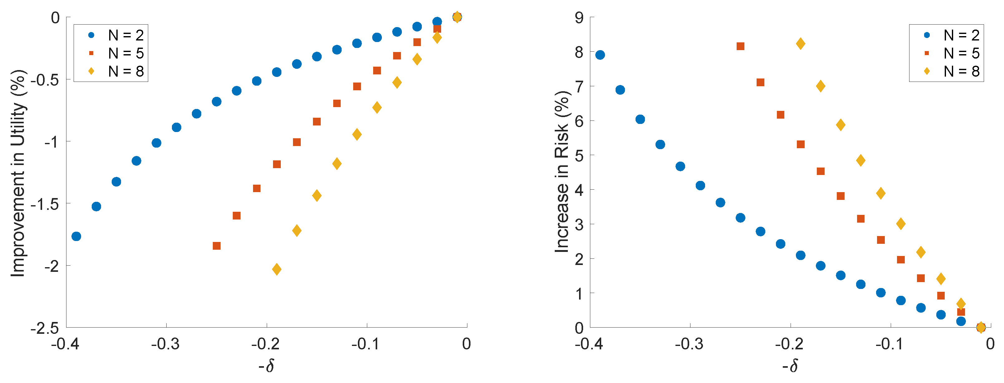
Impact of correlation constraint:Figure 2 depicts the impact of correlation constraint at the terminal expected utility (and risk) for the CSGP strategy relative to the terminal expected utility (and risk) at . We find that a more conservative constraint (higher ) leads to lower utility and higher risk for different values of N. While lower utility for higher is expected, higher risk is driven by increased short position in stocks. For , we find the utility declines by 2% and risk increases by 8% as we increase from to . Longer investment horizon leads to higher reduction in utility and increase in risk due to increased uncertainty in stock price.
Performance in risky environment: Next, we discuss the advantage of CSGP relative to UnSGP strategy as the investment scenario becomes more risky. We consider two risk scenarios: (i) Longer investment horizon (cf. Figure 2) and (ii) Higher correlation of terminal wealth for unconstrained portfolio with the market index.
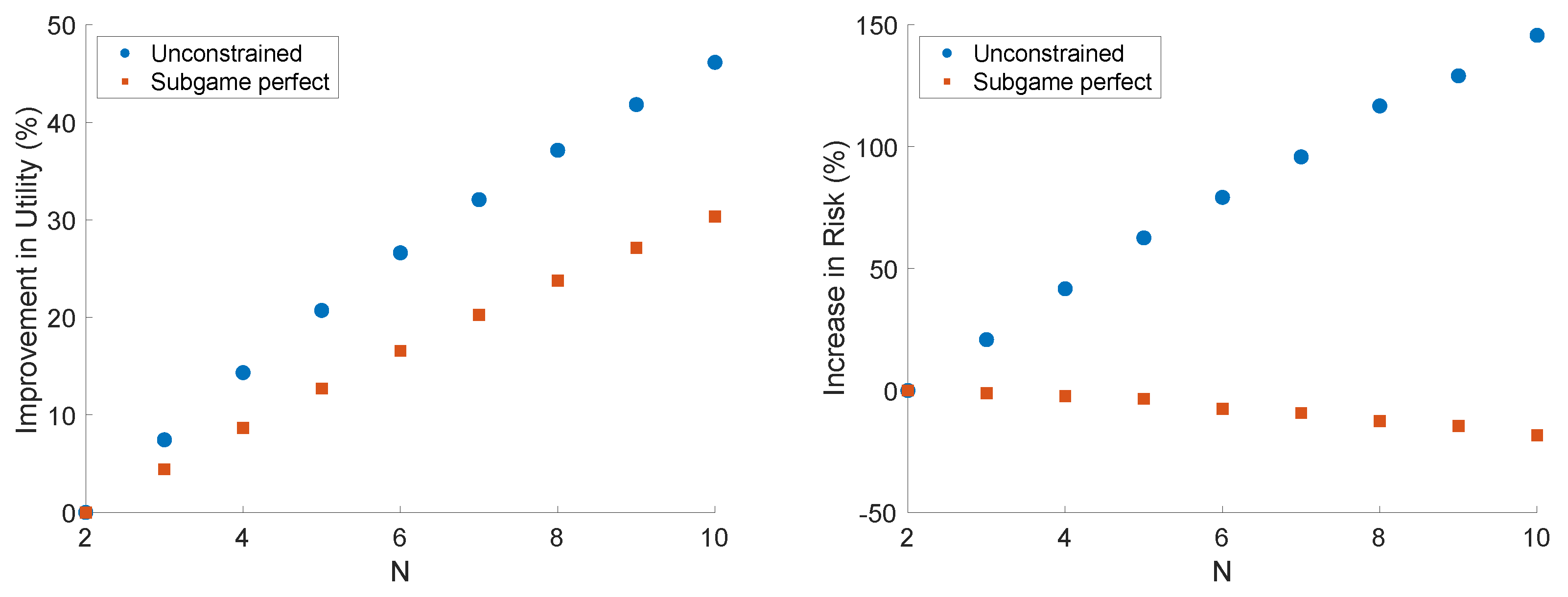
- Longer investment horizon:Figure 3 depicts the impact of investment horizon on the expected terminal utility and risk due to CSGP and UnSGP strategy. The UnSGP strategy leads to 50% increase in expected utility and 150% increase in risk as we increase investment horizon N from 2 to 10. On the contrary, the CSGP strategy leads to only 30% increase in utility but the risk reduces by 18%. Thus for the long investment horizon CSGP strategy not only improves utility but also provides considerable risk reduction.
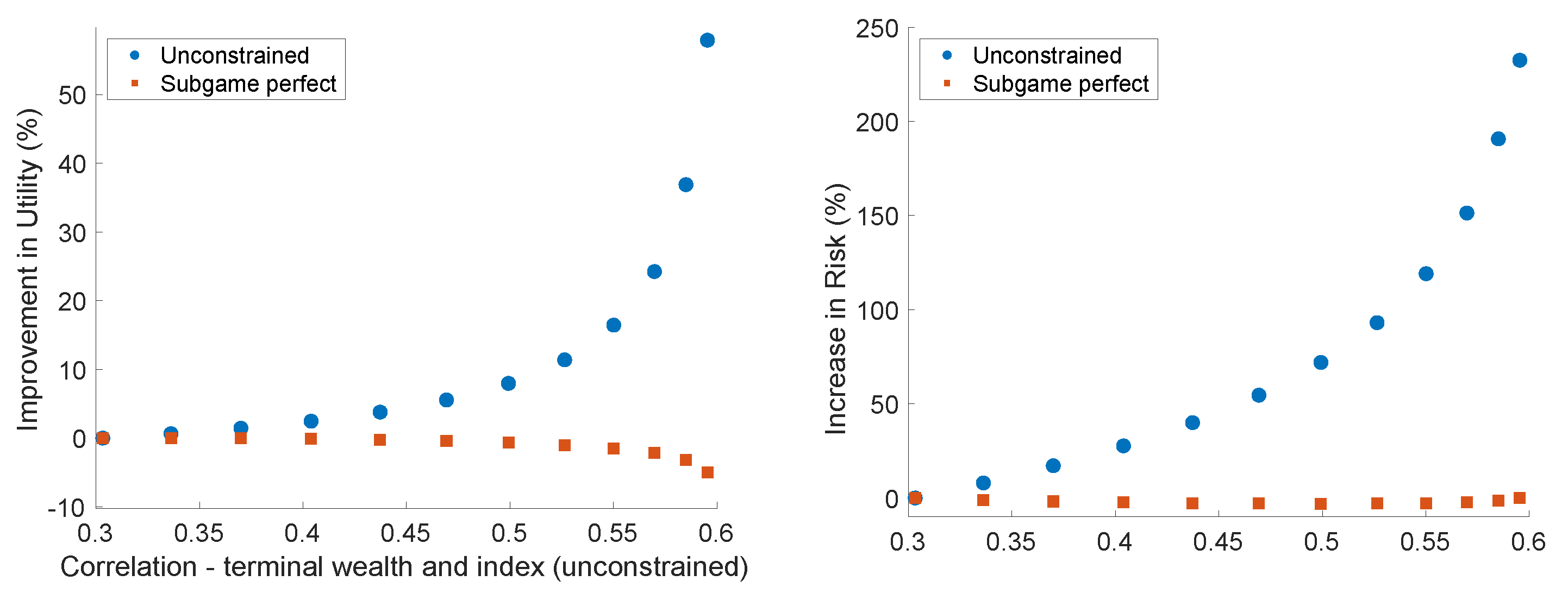
- Higher correlation of unconstrained portfolio wealth with market index:Figure 4 considers the impact of on utility and risk. We consider different scenarios of by changing the volatility of the stock and the index . For simplicity we consider scenarios such that . As increases, the UnSGP strategy provides 55% improvement in utility, however, it results in 250% increase in risk relative to low correlation environment. For such high risk environment, the CSGP strategy provides considerable risk reduction. Unlike UnSGP strategy, here we observe 6% reduction in risk at the expense of 5% loss of utility.
6. Concluding Remarks
We study the impact of correlation constraint on a portfolio optimization problem of one stock and stochastic income stream in a discrete multi-period setting. The constraint represents the correlation of the wealth of the portfolio with a benchmark index representing the state of the economy. The non-linearity due to correlation constraint results in the time inconsistency of the optimal portfolios. A solution to this time consistency issue is the subgame perfect (CSGP) strategy introduced through backward induction. This strategy considers the portfolio problem as a non-cooperative game between players at each time point. We compare the performance of the CSGP strategy to the constrained precommitment (CPC) and the unconstrained subgame perfect (UnSGP) strategy. Using numerical simulations we find that the correlation constraint provides significant risk reduction relative to the unconstrained strategy. The reduction in risk compensates for the loss in utility due to the constraint. We also find similar performances of the two constrained strategies CSGP and CPC. Future works aim at extending the model to allow for more than one stock as well as convergence results to a continuous time model.
Author Contributions
A.M. and T.A.P. contributed equally to this work. All authors have read and agreed to the published version of the manuscript.
Funding
This research received no external funding.
Acknowledgments
The views expressed in this article are those of the authors and do not necessarily reflect the views of Bank of America Securities.
Conflicts of Interest
The authors declare no conflict of interest.
Abbreviations
The following abbreviations are used in this manuscript:
| CSGP | Constrained subgame perfect |
| CPC | Constrained precommitment |
| UnSGP | Unconstrained subgame perfect |
Appendix A. Proof of Lemma 15
For defining the correlation we need some fundamental quantities like covariance between , and variance of and . Recall that
Thus, correlation between and conditional on is given by
where, as before,
Appendix B. Proof of Theorem 1
In this section, we derive the optimal investment for the unconstrained problem.
where
Appendix C. Proof of Theorem 2
Proof.
By Lemma 15 it follows that
Thus
Also, Equation (A16) tells us that
To complete the proof it remains to show that
Since,
For the claim , we take a slightly different route. Notice that
Since
Thus, we have proved that
Hence will be the optimal solution whenever , else is the optimal solution. It is easy to observe that
So, there is no admissible trading strategies if □
Appendix D. Proof of Lemma 2
We need some basic results on variance and covariance of terms involved. Straightforward computations lead to,
where . Thus,
Appendix E. Proof of Theorem 3
Proof.
By Lemma 2 it follows that
Thus, the constraint
where Similar to proof of Theorem 2, we conclude this proof by proving that lies between the roots of quadratic equation for all , i.e.,
where and are the roots of the equation , and are given by
We consider two cases (i) and (ii) separately.
CASE I:
Next we prove that Indeed
So, we proved that
CASE II:
For the sake of simplicity, we write Thus,
Next,
Thus, we proved that for both cases
□
Appendix F. Proof of Theorem 4
Proof.
Objective Function: Objective function in Equation (28), in light of the deterministic trading strategies considered, is simplified as follows
Constraints: The constraint on trading strategy is simplified as follows
where , , and A is a symmetrix matrix given by,
The characteristic equation of A is given by
thus A has negative eigenvalues and one positive eigenvalue. Let us first visualize the solution in two dimensions, which will then extend to N dimensions.
Two Dimensions
In two dimensions, the eigen values are and and the constraint on the trading strategies reduces to
Since the objective function and the domain is convex, the first order conditions (FOC) lead to
N-Dimensions
Since A has negative eigen values and one positive eigenvalue, the constraint is a two-sheeted, N-dimensional hyperboloid. Moreover, similar to two dimensions, the constraint also passes through the two cones of the hyperboloid, leading to a convex constraint for the domain. The FOC lead to Let , where . This transformation simplifies the constraints as:
Furthermore, the linear constraint gets transformed as:
Since we have established that the solution exists when, Thus, the solution of the deterministic precomittment strategy is
□
Appendix G. Proof of Theorem 5
Proof.
The proof of the result follows from Theorem 1 and backward induction. □
References
- Bernard, Carole, Dries Cornilly, and Steven Vanduffel. 2018. Optimal portfolios under a correlation constraint. Quantitative Finance 18: 333–45. [Google Scholar] [CrossRef]
- Bernard, Carole, and Steven Vanduffel. 2014. Mean–variance optimal portfolios in the presence of a benchmark with applications to fraud detection. European Journal of Operational Research 234: 469–80. [Google Scholar] [CrossRef]
- Cox, John C., Stephen A. Ross, and Mark Rubinstein. 1979. Option pricing: A simplified approach. Journal of Financial Economics 25: 229–63. [Google Scholar] [CrossRef]
- Kondor, Imre, Gabor Papp, and Fabio Caccioli. 2017. Analytic solution to variance optimization with no short positions. Journal of Statistical Mechanics: Theory and Experiment 2017: 1–29. [Google Scholar] [CrossRef] [Green Version]
- Kwak, Minsuk, Traian A. Pirvu, and Huayue Zhang. 2014. A multiperiod equilibrium pricing model. Journal of Applied Mathematics 2014: 408685. [Google Scholar] [CrossRef]
- Landsman, Zinoviy, Udi Makov, and Tomer Shushi. 2018. A generalized measure for the optimal portfolio selection problem and its explicit solution. Risks 6: 19. [Google Scholar] [CrossRef] [Green Version]
- Markowitz, Harry. 1952. Portfolio selection. Journal of Finance 7: 77–91. [Google Scholar]
- Pirvu, Traian A., and Huayue Zhang. 2013. Utility indifference pricing: A time consistent approach. Applied Mathematical Finance 20: 304–26. [Google Scholar] [CrossRef] [Green Version]
- Pourbabaee, Farzad, Minsuk Kwak, and Traian A. Pirvu. 2016. Risk minimization and portfolio diversification. Quantitative Finance 16: 1325–32. [Google Scholar] [CrossRef] [Green Version]
- von Neumann, John, and Oskar Morgenstern. 1947. Theory of Games and Economic Behavior. Princeton: Princeton University Press. [Google Scholar]
- Wu, Huiling. 2013. Time-consistent strategies for a multiperiod mean-variance portfolio selection problem. Journal of Applied Mathematics 2013: 841627. [Google Scholar] [CrossRef] [Green Version]
| 1. | The symmetric random walk assumption in modeling stock’s return was introduced by Cox et al. (1979). We impose it because of its simplicity. Our results can be slightly modified to account for asymmetric random walks given that we adjust our (positivity) assumptions below. |
Figure 1.
Optimal portfolio investment.

Figure 2.
Impact of on the constrained subgame perfect (CSGP) strategy.

Figure 3.
Impact of investment horizon (N).

Figure 4.
High correlation environment.


Table 1.
Parameters for the simulations.
© 2020 by the authors. Licensee MDPI, Basel, Switzerland. This article is an open access article distributed under the terms and conditions of the Creative Commons Attribution (CC BY) license (http://creativecommons.org/licenses/by/4.0/).
Share and Cite
MDPI and ACS Style
Maheshwari, A.; Pirvu, T.A. Portfolio Optimization under Correlation Constraint. Risks 2020, 8, 15. https://doi.org/10.3390/risks8010015
AMA Style
Maheshwari A, Pirvu TA. Portfolio Optimization under Correlation Constraint. Risks. 2020; 8(1):15. https://doi.org/10.3390/risks8010015
Chicago/Turabian StyleMaheshwari, Aditya, and Traian A. Pirvu. 2020. "Portfolio Optimization under Correlation Constraint" Risks 8, no. 1: 15. https://doi.org/10.3390/risks8010015
Note that from the first issue of 2016, this journal uses article numbers instead of page numbers. See further details here.