Inverse and Forward Kinematic Analysis of a 6-DOF Parallel Manipulator Utilizing a Circular Guide

Abstract

The proposed study focuses on the inverse and forward kinematic analysis of a novel 6-DOF parallel manipulator with a circular guide. In comparison with the known schemes of such manipulators, the structure of the proposed one excludes the collision of carriages when they move along the circular guide. This is achieved by using cranks (links that provide an unlimited rotational angle) in the manipulator kinematic chains. In this case, all drives stay fixed on the base. The kinematic analysis provides analytical relationships between the end-effector coordinates and six controlled movements in drives (driven coordinates). Examples demonstrate the implementation of the suggested algorithms. For the inverse kinematics, the solution is found given the position and orientation of the end-effector. For the forward kinematics, various assembly modes of the manipulator are obtained for the same given values of the driven coordinates. The study also discusses how to choose the links lengths to maximize the rotational capabilities of the end-effector and provides a calculation of such capabilities for the chosen manipulator design.

1. Introduction

Currently, manipulators designed with a parallel structure are becoming more widespread in technology. Many different types of these manipulators are known and they provide exceptional functional properties [1,2,3,4]. Herein parallel manipulators equipped with a circular guide are quite promising for practical application. Their kinematic chains are supported by movable carriages, which allow chains to switch the position of the end-effector relative to a fixed link designed as a circular guide [5,6].

A circular guide provides the end-effector with a large rotational angle around the vertical axis that is quite an important property for many practical applications. In addition, the design features of manipulators with a circular guide ensure the manipulation of heavy objects. Due to the possibility of realization of these important functional properties, such manipulators have become the object of many studies in recent years.

The first parallel manipulator with a circular guide was mentioned in [7] in 1983. This is a six-degree-of-freedom (6-DOF) manipulator, in which six kinematic chains couple in pairs at the end-effector (platform). This manipulator provides a full range of motions of the end-effector with complete rotation around the vertical axis, and it has three additional mobilities that do not affect the trajectories of the end-effector. The kinematics of this manipulator and its workspace analysis are presented in [8]. Later, similar kinematic schemes of 6-DOF parallel manipulators, including exclusively joints with rotational DOFs, were presented in [9,10,11,12,13].

An advanced scheme of the 6-DOF manipulator with a circular guide [7] is presented in [14]. A study of its kinematics and working zone analysis is presented in [15]. A similar manipulator with kinematic chains having different types of joints, including universal joints, is presented in [16].

A different structure of the 6-DOF manipulator with a circular guide is proposed in [17,18]. The manipulator designed with three kinematic chains and equipped with prismatic joints, which allow the manipulator to have large displacement along the vertical axis. A 3-DOF manipulator with a circular guide is shown in [19]. It was designed on the basis of spherical kinematic chains. Its principal difference from the spherical manipulator is in increased rotational angle around the vertical axis. In [20], this manipulator is presented with a reconfigurable kinematic design that allows changing the size of its working zone. Another variation of the 3-DOF spherical manipulator with a circular guide proposed in [21]. The manipulator includes kinematic chains 3-RUS and 1-S. In [22], a manipulator with a circular guide is presented as a 1-DOF system. The transition from six drives to one is realized by installing an additional lever mechanism inside the circular guide, which provides the dependent movement of all carriages from a single drive. All of the above discussed manipulators with a circular guide, with the exception of the manipulator given in [22], have drives mounted exclusively on the movable links (carriages). Moreover, the structure of these manipulators is organized in such a way that the possibility of collision between the adjacent carriages is not eliminated.

In this regard, the proposed study aims at the designing and analysis of such a manipulator with a circular guide that provides placement of all drives fixed on the base, ensures elimination of the possibility of collision between the adjacent carriages while having a sufficiently large rotation of the end-effector around the vertical axis and providing six DOFs.

2. Manipulator Architecture

Let us consider the structure and functional features of the proposed 6-DOF manipulator with a circular guide. Figure 1 presents its CAD (computer-aided design) model (virtual prototype). The model allows not only to fabricate its physical prototype but also to perform numerical calculations and experiments. The operation of the CAD model is presented in the movie in Supplementary Materials. The key elements in Figure 1 are: 1—circular guide (fixed link); 2—drive; 3—crank; 4—slide block; 5—swinging arm; 6—carriage; 7—leg; 8—platform (end-effector). Slide block 4 and swinging arm 5 form a prismatic joint, swinging arm 5 and carriage 6 form a single link (rigid connection), leg 7 is connected on both sides with carriage 6 and platform 8 by spherical joints. Figure 1 also demonstrates the main constructive assemblies of the manipulator: I—the coupling of leg 7 and platform 8 through spherical joints; II—the coupling of six swinging arms 5, which converge in the center of circular guide 1 and have a common rotational axis; III—the coupling of links 1–6.

In each of the six kinematic chains of the manipulator, the input motions pass from cranks 2 to slide blocks 4 and then to swinging arms 5, turning them at certain angles. Swinging arms 5 displace carriages 6 along circular guide 1. The motion transmits to legs 7 and then to platform 8. Thus, six independently actuated kinematic chains provide the change of position and orientation of platform 8.

One can note the following design features of the proposed manipulator:

• all drives stay fixed on the base;
• correctly chosen cranks’ lengths allow eliminating the possibility of collision between the adjacent carriages;
• sufficiently large rotation of the end-effector around the vertical axis.

3. Kinematic Analysis

Let us consider the solution of the inverse and forward position problems, which allows to identify the relationships between the end-effector coordinates and the controlled movements in the manipulator drives. In this case, the inverse problem aims at calculating the driven coordinates for the given end-effector coordinates, and the forward one aims at determining the position and orientation of the end-effector with known driven coordinates.

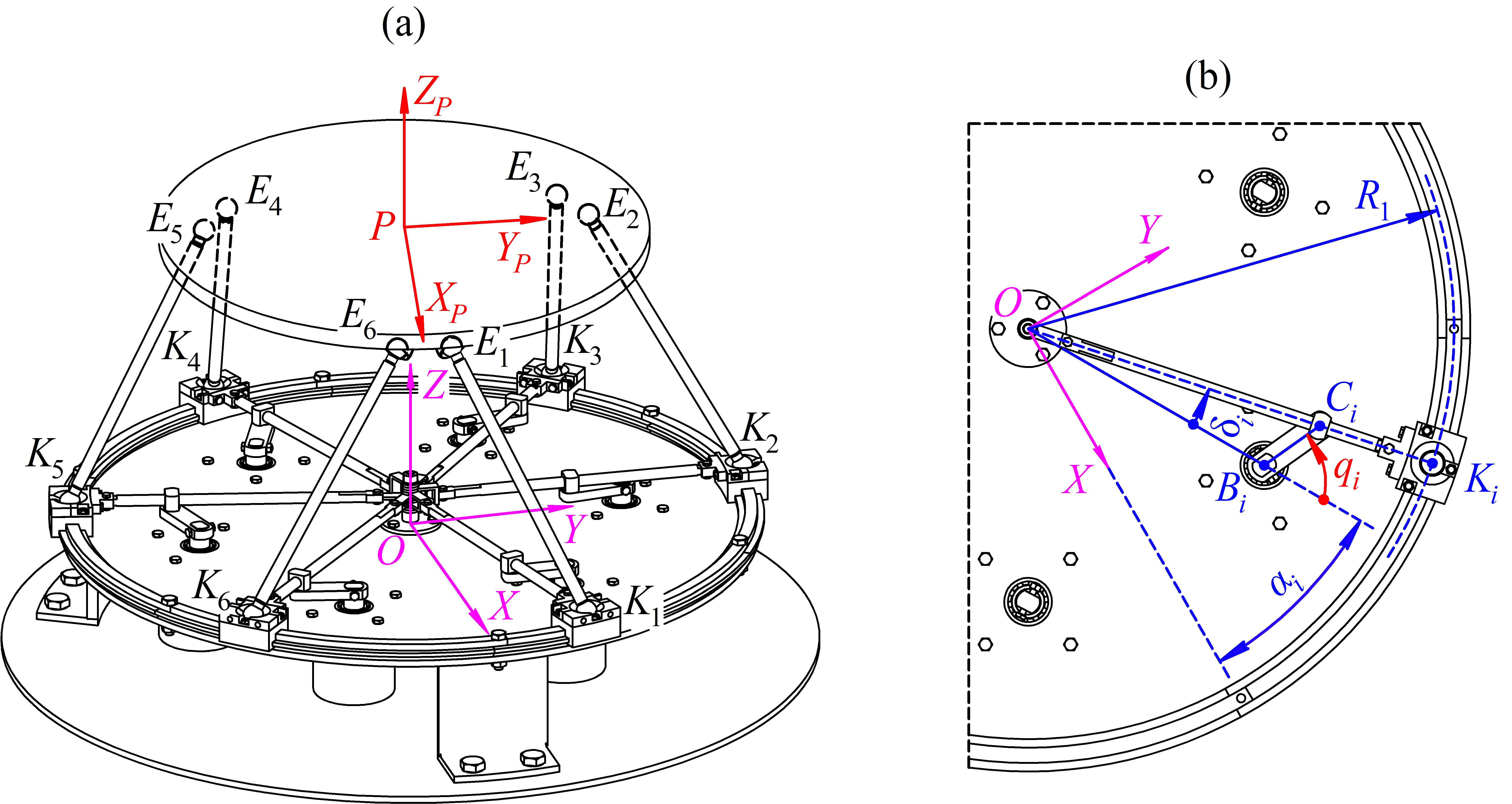
The position of the end-effector can be described by the Cartesian coordinates of any of its points, for example, its center, point P (Figure 2a). These coordinates can be represented as vector p_P that determines the position of point P relative to global coordinate system OXYZ. Plane OXY is in the plane of carriages K_i, i = 1 … 6, and the center, point O, corresponds to the intersection point of the circular guide axis with this plane. The end-effector orientation can be set using rotation matrix R_P, which determines the orientation of local coordinate system PX_PY_PZ_P attached to the end-effector relative to global coordinate system OXYZ.

Let us represent the driven coordinates of the manipulator as vector q:

$$q={\left[q_1{ q}_2{ q}_3 q_4{ q}_5{ q}_6\right]}^{\mathrm{T}},$$

(1)

where q_i corresponds to the rotational angle of i-th crank, i = 1 … 6 (Figure 2b).

3.1. Inverse Kinematics

The solution of the inverse position problem is to find driven coordinates q for given vector p_P and matrix R_P, which describe the end-effector position and orientation. The algorithm for solving this problem is as following. Coordinates p_Ei of points E_i (the centers of spherical joints 7–8), i = 1 … 6, relative to global coordinate system OXYZ can be written as:

$${\mathbf{p}}_{Ei} = {\mathbf{p}}_P{ + \mathbf{R}}_P{\mathbf{r}}_{Ei},$$

(2)

where r_Ei are the coordinates of points E_i in local coordinate system PX_PY_PZ_P.

Coordinates p_Ki of points K_i (the centers of spherical joints 6–7), i = 1 … 6, in global coordinate system OXYZ can be found in the following way:

$${\mathbf{p}}_{Ki}={\left[\begin{array}{ccc}{R}_1\cos \left({\mathsf{\alpha }}_i{+\mathsf{\delta }}_i\right)& R_1\sin \left({\mathsf{\alpha }}_i{+\mathsf{\delta }}_i\right)& 0\end{array}\right]}^{\mathrm{T}},$$

(3)

where R₁ is the radius of circular guide 1; α_i is the angle between axis OX and line OB_i (Figure 2b); δ_i is the rotational angle of i-th swinging arm 5.

Let us write the relationship, linking coordinates of points E_i and K_i with length L_i of leg 7:

$${\left({\mathbf{p}}_{Ei}-{\mathbf{p}}_{Ki}\right)}^2{=L}_i^2,$$

(4)

After substituting Equations (2) and (3) in Equation (4) and carrying out transformations, the following relation can be obtained:

$$p_{Ei}^x\cos \left({\mathsf{\alpha }}_i{+\mathsf{\delta }}_i\right)+p_{Ei}^y\sin \left({\mathsf{\alpha }}_i{+\mathsf{\delta }}_i\right)=\frac{{\mathbf{p}}_{\mathit{Ei}}^2+R_1^2-L_i^2}{2R_1},$$

(5)

where p_Ei^x and p_Ei^y are the corresponding components of vector p_Ei.

Angle δ_i of swinging arm 5 is an unknown parameter in Equation (5). Let us apply the tangent half-angle substitution to find this angle:

$$\cos \left({\mathsf{\alpha }}_i{+\mathsf{\delta }}_i\right)=\frac{1-t_i^2}{1+t_i^2}, \sin \left({\mathsf{\alpha }}_i{+\mathsf{\delta }}_i\right)=\frac{2t_i}{1+t_i^2}, t_i=\tan \left(\frac{{\mathsf{\alpha }}_i+{\mathsf{\delta }}_i}{2}\right).$$

(6)

Substituting Equation (6) into Equation (5), after transformations, the following expression can be obtained:

$$a_i{t}_i^2+b_i{t}_i+c_i=0.$$

(7)

Coefficients a_i, b_i, and c_i are known when solving the inverse position problem. In the general case, quadratic Equation (7) can have two solutions, which can be interpreted as follows. The motion trajectory of each carriage (point K_i) is a circle. At the same time, for the given (fixed) coordinates of the end-effector, point K_i must be on the surface of the sphere with the center at point E_i and radius L_i. This sphere generally has two intersection points with the mentioned circle that corresponds to quadratic Equation (7). The choice of the specific solution is determined by the design features of the manipulator.

After determining variable t_i, angle δ_i of swinging arm 5 can be found from Equation (6) written as follows:

$${\mathsf{\delta }}_i=2\arctan \left(t_i\right)-{\mathsf{\alpha }}_i.$$

(8)

The angle at apex C_i of triangle OB_iC_i can be determined using the sine theorem as:

$$\angle {OC}_i{B}_i=\arcsin \left(\frac{d_i{\sin \mathsf{\delta }}_i}{l_i}\right).$$

(9)

where d_i is the distance between point O and rotational axis B_i of i-th crank (Figure 2b); l_i is the length of i-th crank.

Finally, the rotational angle of the i-th crank, i.e., the value of driven coordinate q_i, can be determined:

$$q_i{=\mathsf{\delta }}_i+\angle {OC}_i{B}_i.$$

(10)

Thus, the solution of the inverse position problem has been found. The solution algorithm is the same for all kinematic chains of the manipulator.

3.2. Forward Kinematics

The solution of the forward position problem for the proposed manipulator is to find vector p_P and rotation matrix R_P, which describes the end-effector position and orientation, for given driven coordinates q. The algorithm for solving this problem is as follows.

Initially, length OC_i (i = 1 … 6) can be found using the cosine theorem for triangle OB_iC_i (Figure 2b):

$$O{C}_i=\sqrt{d_i^2+l_i^2+2d_i{l}_i\cos q_i}.$$

(11)

Next, angle δ_i of swinging arm 5 can be determined using the sine theorem for the same triangle:

$${\mathsf{\delta }}_i = \arcsin \left(\frac{l_i\sin q_i}{O{C}_i}\right).$$

(12)

Then, Equation (3) allows to find coordinates p_Ki of carriages 6. As a result, a system of six equations of the form (4) can be written. With Equation (2), this system has twelve unknown variables: three components of vector p_P and nine components of matrix R_P. Since rotation matrix R_P is orthogonal, the following additional relations exist [23]:

$${\left|u\right|}^2=1, {\left|v\right|}^2=1, u·\mathbf{v}=0, u\times \mathbf{v}=\mathbf{w},$$

(13)

where u, v, and w are the columns of matrix R_P:

$$R_P = \left[\begin{array}{ccc}u& v& w\end{array}\right].$$

(14)

Thus, six equations of the form (4) and six equations of the form (13) represent a system of twelve equations with respect to twelve variables. All the equations are second-degree polynomials. Such a system of equations is inherent for many parallel mechanical systems, including the classical Gough-Stewart platform [23], and the determination of its solutions in an explicit form comes with significant computational difficulties. Many authors have proposed various algorithms for solving these equations based on the methods of dialytic elimination [24], homotopy continuation [25], Gröbner bases [26], interval analysis [27], and others [28,29]. The studies above showed that in general (in the case of an arbitrarily chosen geometry of the manipulator), the system can have 40 different solutions, both real and complex, and Husty [30] provided an algorithm to form a univariate polynomial of 40th degree that allows finding all the solutions. Dietmaier also showed that all the solutions can be the real ones [31]. Any of the approaches above can be applied to solve the system of equations discussed in this study. The next section will discuss the examples of solving both position problems.

3.3. Examples of Kinematic Problems’ Solution

Let us consider examples of solving the inverse and forward position problems for the manipulator with the following parameters, corresponding to the CAD model (Figure 1): radius of circular guide 1, R₁ = 250 mm; length of crank 3, l_i = 40 mm, i = 1 … 6; length of leg 7, L_i = 222 mm, i = 1 … 6; distance between points O and B_i, d_i = 160 mm, i = 1 … 6; angle between axis OX and length OB_i, α_i = 30°, 90°, 150°, 210°, 270°, 330°; coordinates of spherical joints 7–8 in local coordinate system PX_PY_PZ_P, ${\mathbf{r}}_{Ei}={\left[\begin{array}{ccc}{R}_8{\cos \mathsf{\beta }}_i& R_8{\sin \mathsf{\beta }}_i& 0\end{array}\right]}^{\mathrm{T}}$, where R₈ = 153 mm is the radius of platform 8; β_i is the angular placement of joints 7–8, β_i = 7.5°, 112.5°, 127.5°, 232.5°, 247.5°, 352.5°.

3.3.1. Example of Inverse Position Problem Solution

First, consider an example of solving the inverse position problem for the simplest case, when point P of the end-effector is located above point O at height 180 mm. Let the axes of local coordinate system PX_PY_PZ_P be aligned with the axes of coordinate system OXYZ, i.e., rotation matrix R_P is identity in this case. As a result of the calculation according to the above mentioned algorithm, implemented in MATLAB package, the following values of the driven coordinates were determined:

$$q={\left[\begin{array}{cccccc}15.3°& -15.3°& 15.3°& -15.3°& 15.3°& -15.3°\end{array}\right]}^{\mathrm{T}}.$$

(15)

The rotational angles of cranks form two groups with equal values and opposite in sign: q₁ = q₃ = q₅ = −q₂ = −q₄ = −q₆. As expected, the solution has certain “symmetry”, which is fully consistent with the “symmetric” geometry and the given configuration of the manipulator.

3.3.2. Example of Forward Position Problem Solution

Next, consider an example of solving the forward position problem, taking Equation (15) as the given values of the driven coordinates. This problem was solved by the homotopy continuation method [32] that implies the following idea. Given the system of equations to solve in a standard form F(X) = 0, one can form an auxiliary system:

$$H\left(X,\lambda \right)=\left(1-\lambda \right)G\left(X\right)+\lambda F\left(X\right)=0,$$

(16)

where G(X) is a system that has the same number of solutions as F(X), and all these solutions are known; λ is a scalar parameter, varying from 0 to 1.

When λ = 0, H(X, 0) = G(X), and all the solutions are known. These solutions present an initial guess to solve a new version of H(X, λ) with slightly increased value of λ using standard iterative algorithms. The process is repeated until λ = 1, for which H(X, 1) = F(X). Thus, the starting system G(X) = 0 with known solutions slowly evolves toward the desired one F(X) = 0.

As mentioned before, system F(X) = 0 for the studied manipulator consists of twelve second-order degree polynomials with respect to twelve variables. According, to Bezout’s theorem [33], this system can have a maximum of 2¹² = 4096 solutions. Given this, one can form the system G(X) = 0 with the desired number of solutions.

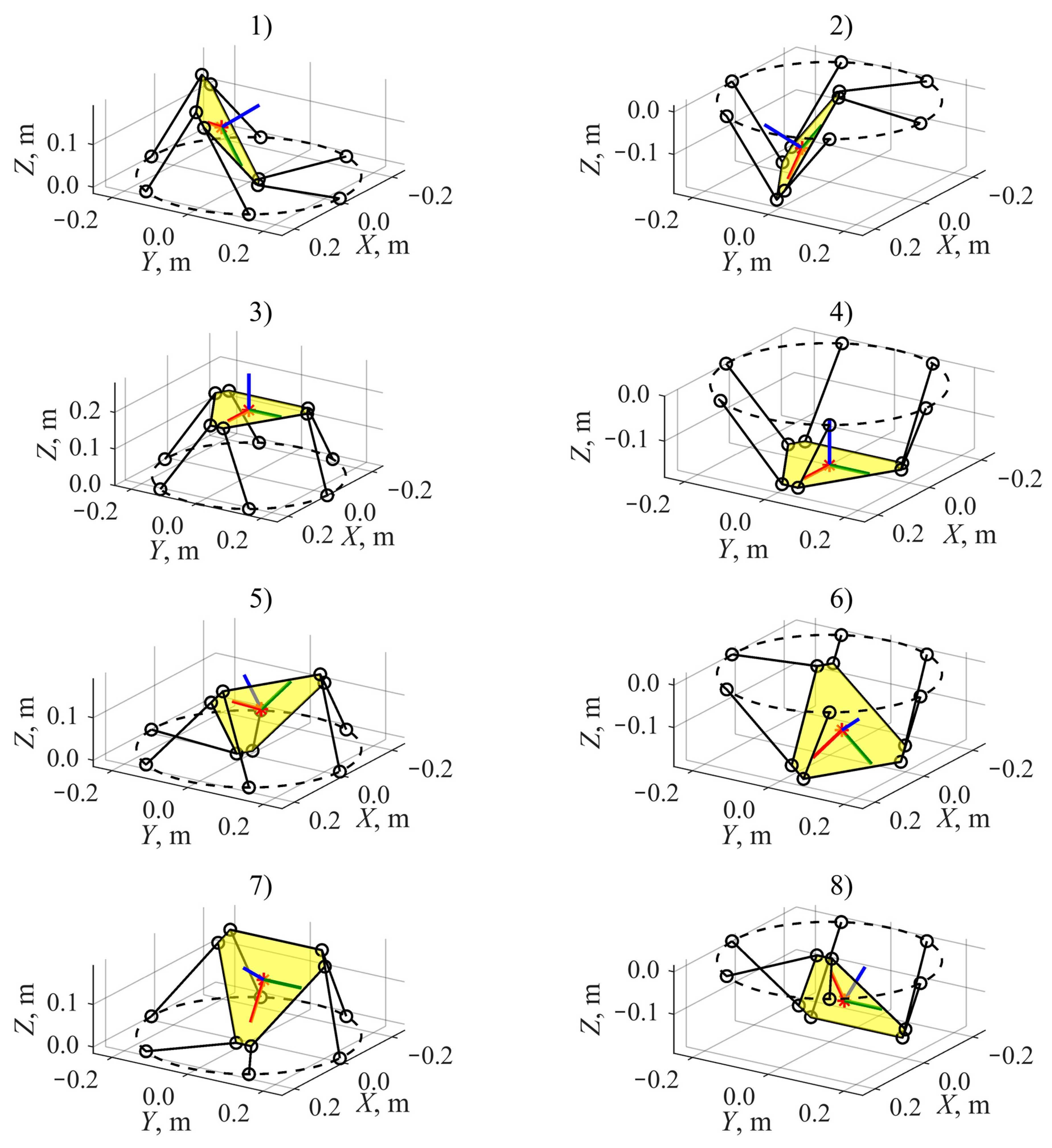
This procedure was realized automatically using Bertini program [34], implemented in MATLAB package as BertiniLab interface [35]. As a result, 28 different solutions were obtained: 8 real and 20 complex. These eight real solutions correspond to eight different assembly modes of the manipulator and are shown in

Table 1. The Results of Solving the Forward Position Problem.

	Solution Number
	1	2	3	4
pP, mm	$\left[\begin{array}{c}30.39\\ -52.63\\ 113.19\end{array}\right]$	$\left[\begin{array}{c}30.39\\ -52.63\\ -113.19\end{array}\right]$	$\left[\begin{array}{c}0.00\\ 0.00\\ 180.00\end{array}\right]$	$\left[\begin{array}{c}0.00\\ 0.00\\ -180.00\end{array}\right]$
RP	$\left[\begin{array}{ccc}0.88& 0.20& -0.42\\ 0.20& 0.65& 0.73\\ 0.42& -0.73& 0.54\end{array}\right]$	$\left[\begin{array}{ccc}0.88& 0.20& 0.42\\ 0.20& 0.65& -0.73\\ -0.42& 0.73& 0.54\end{array}\right]$	$\left[\begin{array}{ccc}1.00& 0.00& 0.00\\ 0.00& 1.00& 0.00\\ 0.00& 0.00& 1.00\end{array}\right]$	$\left[\begin{array}{ccc}1.00& 0.00& 0.00\\ 0.00& 1.00& 0.00\\ 0.00& 0.00& 1.00\end{array}\right]$
	Solution Number
	5	6	7	8
pP, mm	$\left[\begin{array}{c}30.39\\ 52.63\\ 113.19\end{array}\right]$	$\left[\begin{array}{c}30.39\\ 52.63\\ -113.19\end{array}\right]$	$\left[\begin{array}{c}-60.77\\ 0.00\\ 113.19\end{array}\right]$	$\left[\begin{array}{c}-60.77\\ 0.00\\ -113.19\end{array}\right]$
RP	$\left[\begin{array}{ccc}0.88& -0.20& -0.42\\ -0.20& 0.65& -0.73\\ 0.42& 0.73& 0.54\end{array}\right]$	$\left[\begin{array}{ccc}0.88& -0.20& 0.42\\ -0.20& 0.65& 0.73\\ -0.42& -0.73& 0.54\end{array}\right]$	$\left[\begin{array}{ccc}0.54& 0.00& 0.84\\ 0.00& 1.00& 0.00\\ -0.84& 0.00& 0.54\end{array}\right]$	$\left[\begin{array}{ccc}0.54& 0.00& -0.84\\ 0.00& 1.00& 0.00\\ 0.84& 0.00& 0.54\end{array}\right]$

Notice: the data are presented accurate to two decimals.

and Figure 3. Assembly mode #3 corresponds to the specified end-effector configuration from the previous example. Note that half of the assemblies have a symmetrical analog located on the other side of plane OXY.

One should also notice that the number of obtained solutions, 28, is less than 40. The reason is that the considered manipulator has a “symmetrical” geometry and the example was performed for “symmetrical” values of the driven coordinates. In the general case, the number of solutions will be equal to 40.

4. Geometrical Analysis

4.1. Calculation of Crank Lengths

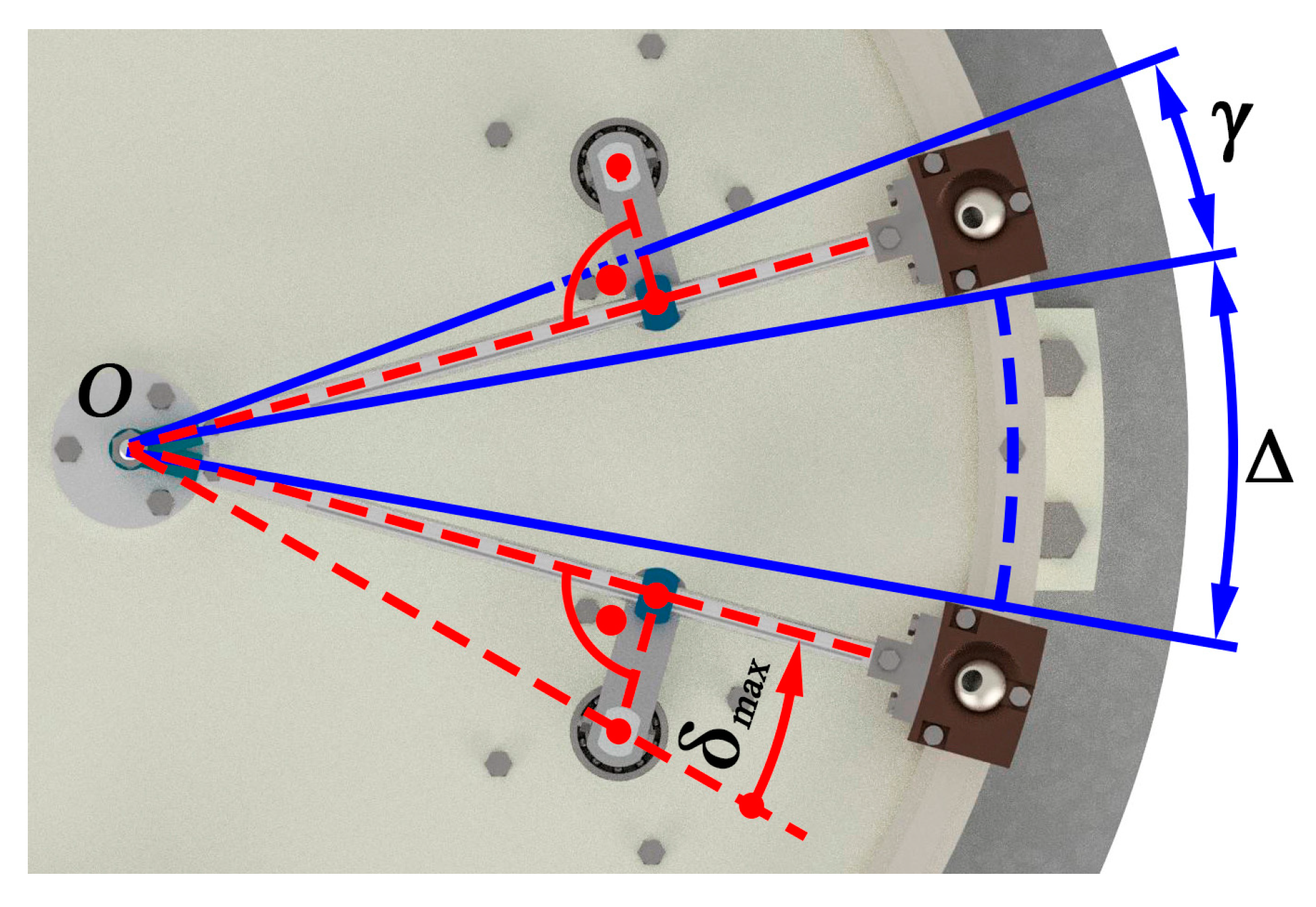
As mentioned in Section 2, the correctly chosen cranks lengths allow eliminating the possibility of collision between the adjacent carriages. Let us address this problem in detail. Let’s consider the symmetrical geometry of the manipulator as in the previous examples: all the cranks have length l and their rotational axes are located evenly on a circle with radius d. Suppose that the carriages have angular width γ, and the distance between the adjacent carriages when they are in extreme positions is Δ (Figure 4). In this configuration, each crank is perpendicular to the corresponding swinging arm. Each of the arms rotate on its maximum angle δ_max, so:

$${\sin \mathsf{\delta }}_{max}=l/d.$$

(17)

On the other hand, according to Figure 4:

$$2\left({\mathsf{\delta }}_{max}+\frac{\mathsf{\gamma }}{2}\right)+\mathsf{\Delta }=\mathsf{\pi }/3.$$

(18)

Combining Equations (17) and (18), one can find the crank length:

$$l=d\sin \left(\frac{\mathsf{\pi }}{6}-\frac{\mathsf{\Delta }+\mathsf{\gamma }}{2}\right).$$

(19)

The equation above allows finding the crank length for the specified gap Δ between the carriages. For example, for d = 160 mm as in Section 3.3, γ = 10°, and Δ = 0 (extreme case), the crank length will be l = 67.6 mm.

4.2. Calculation of Maximum Rotational Angle of the Platform

The key feature of manipulators with a circular guide is the ability to provide large rotational angles around the vertical axis. Let us calculate these angles for the proposed manipulator in the following way.

For simplicity, suppose that the platform’s plane is parallel to the base one, and the platform’s center stays above the center of the base. For the proposed manipulator, these assumptions can be written as:

$$p_P=\left[\begin{array}{c}0\\ 0\\ z\end{array}\right], R_P=\left[\begin{array}{ccc}\cos \mathsf{\phi }& -\sin \mathsf{\phi }& 1\\ \sin \mathsf{\phi }& \cos \mathsf{\phi }& 0\\ 0& 0& 0\end{array}\right],$$

(20)

where z is the height of the platform above the base; φ is the rotational angle of the platform around the vertical axis.

In addition, suppose that the platform’s spherical joints are placed on radius R₈ with angular coordinates β_i as in the previous examples, i.e., ${\mathbf{r}}_{Ei}={\left[\begin{array}{ccc}{R}_8{\cos \mathsf{\beta }}_i& R_8{\sin \mathsf{\beta }}_i& 0\end{array}\right]}^{\mathrm{T}}$, i = 1 … 6. With these assumptions, Equation (5) can be transformed to the following form:

$$R_8\cos \left(\mathsf{\phi }+{\mathsf{\beta }}_i-{\mathsf{\alpha }}_i-{\mathsf{\delta }}_i\right)=\frac{z^2+R_8^2+R_1^2-L_i^2}{2R_1}.$$

(21)

The equation above allows to express angle φ:

$$\mathsf{\phi }={\mathsf{\delta }}_i+{\mathsf{\alpha }}_i-{\mathsf{\beta }}_i\pm \arccos \left(\frac{z^2+R_8^2+R_1^2-L_i^2}{2R_1{R}_8}\right).$$

(22)

The choice of the sign is determined by the design features of the kinematic chains. Equation (22) can be used to estimate the maximum value of angle φ permitted by each of the six chains. Given the manipulator geometry, this value mainly depends on the maximum rotational angles δ_imax of the swinging arm, and platform’s height z:

$${\mathsf{\phi }}_{imax}={\mathsf{\delta }}_{imax}+{\mathsf{\alpha }}_i-{\mathsf{\beta }}_i\pm \arccos \left(\frac{z^2+R_8^2+R_1^2-L_i^2}{2R_1{R}_8}\right).$$

(23)

The value of δ_imax can be found using Equation (17). Since each of the kinematic chains can permit different values of maximum rotational angle φ_imax, one has to choose the minimum one over all kinematic chains:

$${\mathsf{\phi }}_{max}={\min }_{i=1 \dots 6}\left({\mathsf{\phi }}_{imax}\right).$$

(24)

A similar procedure can be used to find the minimum value of angle φ concerning the minimum rotational angle δ_imin of the swinging arm:

$${\mathsf{\phi }}_{imin}={\mathsf{\delta }}_{imin}+{\mathsf{\alpha }}_i-{\mathsf{\beta }}_i\pm \arccos \left(\frac{z^2+R_8^2+R_1^2-L_i^2}{2R_1{R}_8}\right),$$

(25)

and

$${\mathsf{\phi }}_{min}={\max }_{i=1 \dots 6}\left({\mathsf{\phi }}_{imin}\right).$$

(26)

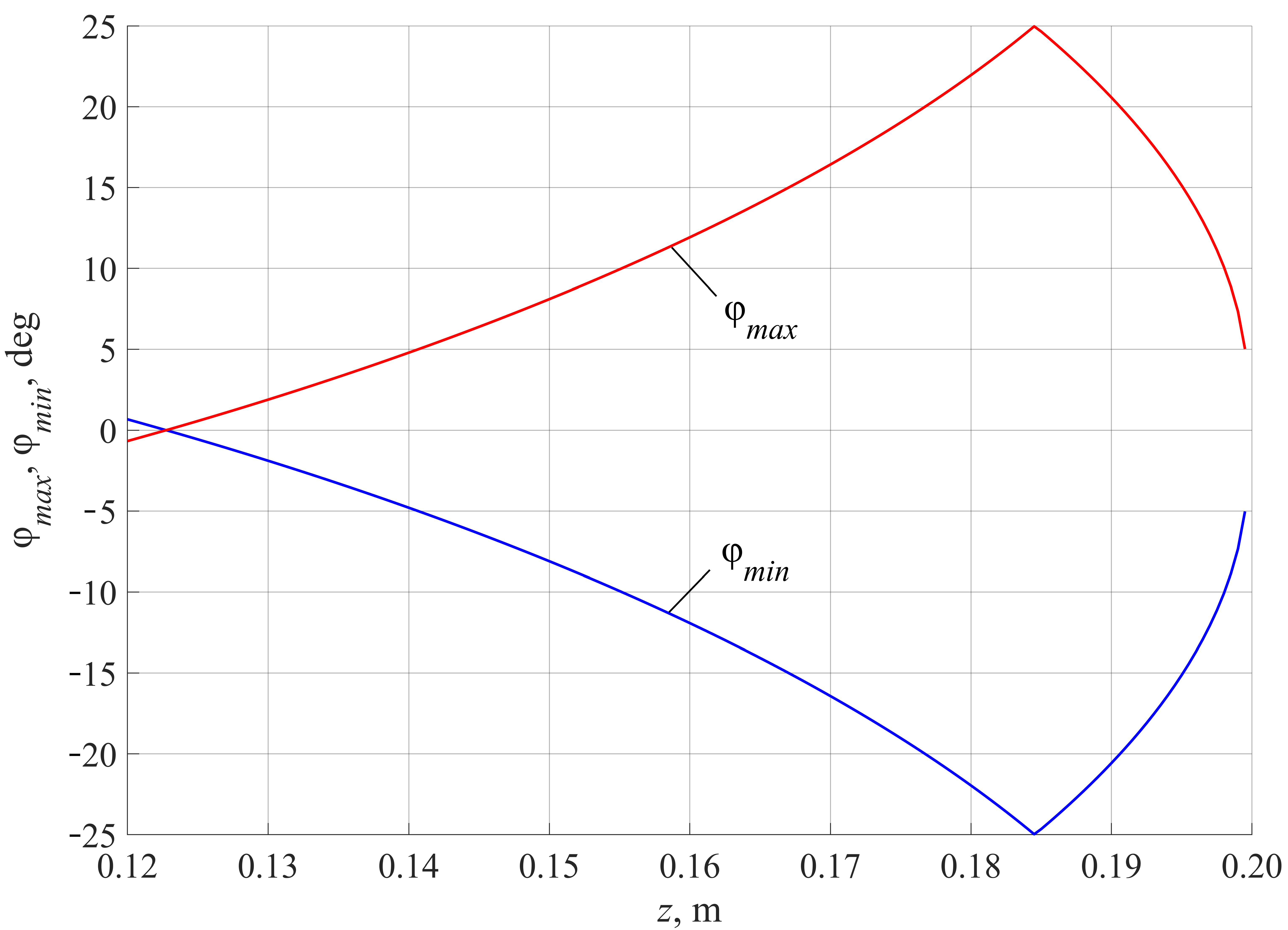
The proposed procedure has been modeled in MATLAB for the manipulator with the same parameters as above, except crank length, which was set to 67.6 mm. Figure 5 demonstrates the dependence of angles φ_min and φ_max on the platform’s center coordinate z, which varies between 120 and 200 mm. Due to the symmetrical geometry of the manipulator, φ_min = −φ_max. For smaller values of coordinate z, φ_min becomes greater than φ_max, and these configurations are not acceptable. For higher values of coordinate z, there are no values of φ_min and φ_max since the manipulator cannot be in those configurations. The maximum value of φ_max is equal to 25° for coordinate z near 185 mm.

The extreme values of angle φ are smaller than the ones for the classical Gough-Stewart platform that can reach about 60° [36,37]. However, with Equations (23)–(26), one can formulate an optimization problem to find mechanism geometry that will maximize the range of rotation. Another solution is to change the manipulator structure and use two circular guides: one of them is inside the other (as in [38]) or stacked over it. Each guide will support only three carriages increasing their driving range and, therefore, the rotational capabilities of the platform.

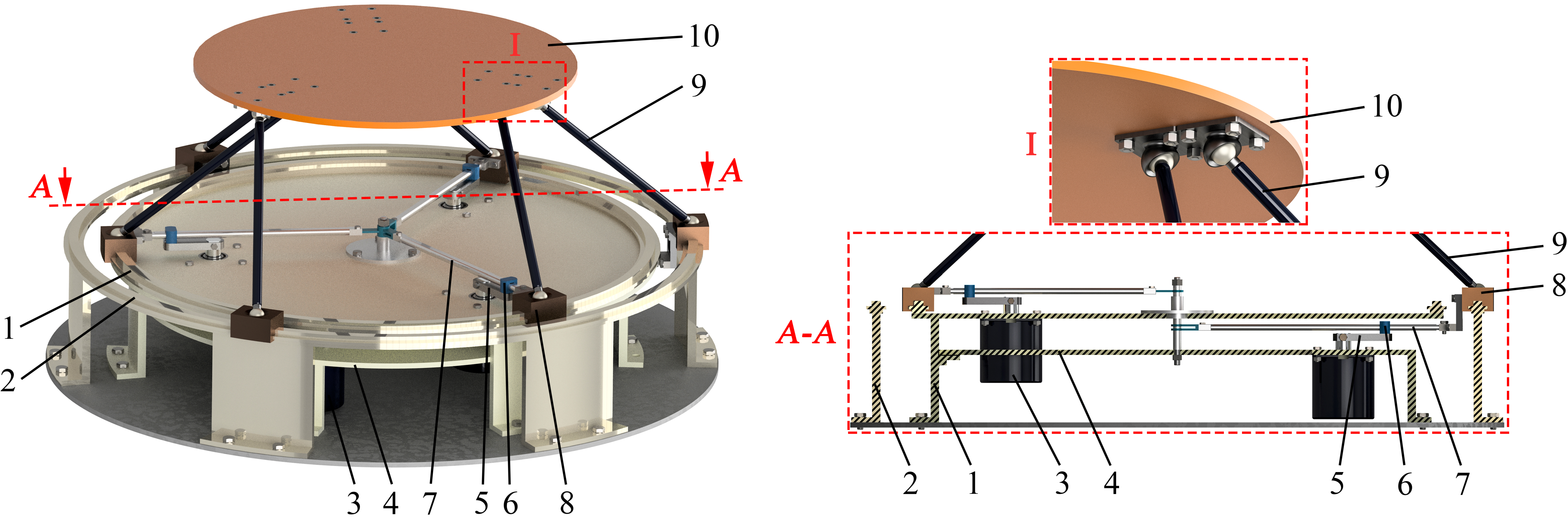
Figure 6 presents such a variation of the proposed design with two circular guides. The swinging arms can rotate at higher angles leading to the increased value of platform rotational angle φ. Here are: 1—inner circular guide (fixed link); 2—outer circular guide (fixed link); 3—drive; 4—support for drive 3; 5—crank; 6—slide block; 7—swinging arm; 8—carriage; 9—leg; 10—platform (end-effector). The proposed design requires location of the centers of spherical joints 9–10 according to view I in Figure 6, where each pair of these joints is on the same radius of the platform. To provide higher rotational angle φ, three kinematic chains of links 5–7 are moved under the circular guides (section A-A in Figure 6). For the presented design, the maximum value of rotational angle φ is about 55°, which is comparable to the Gough-Stewart platform.

Both proposed designs in Figure 1 and Figure 6 can be further optimized to enhance the rotational capabilities of the platform, not only in one particular configuration but over the whole working area. This topic is beyond the current study but presents interest for future research.

5. Conclusions

This study has presented a novel version of the 6-DoF manipulator with a circular guide. The proposed manipulator has such design advantages as having all drives fixed on the base, sufficiently large rotation of the end-effector around the vertical axis, and using cranks as the driving links (as an alternative to carriages) placed within the circular guide. The manipulator can find an application for positioning different elements and objects in space.

The study has presented algorithms for solving the inverse and forward kinematics. The former one has a closed-form solution. First, the position of upper and lower spherical joints, as well as carriages, is determined based on the given end-effector coordinates, second, the rotational angles of cranks (driven coordinates) are calculated. The solution of the forward kinematics has been determined using the homotopy continuation method. According to the example, 28 different solutions have been found (8 real and 20 complex) for the same values of the driven coordinates. Eight assembly modes have been obtained according to the eight real solutions. The study has also presented methods for calculation of the rotational capabilities of the platform and for selection of link lengths. It has been found that the platform can rotate from −25° to +25° around the vertical axis with respect to the chosen manipulator design. However, these values can be increased by different design variations. The study has presented another manipulator design with two circular guides, which allows significantly increasing the rotational angle around the vertical axis. In this design, the angle can vary from −55° to +55°, which is comparable to the one of the Gough-Stewart platform.

The work has studied design variations of the manipulator with symmetrical geometry and performed analysis when the platform is parallel to the base and is located right above its center. The techniques proposed in the study can be expanded for other cases too. The kinematic analysis of the manipulator performed in this work can serve as a basis for the further analysis of velocities and accelerations, as well as workspace analysis and optimal design. In addition, the singularities that can affect the shape and size of the workspace of the manipulator are of special interest.

References

- Ceccarelli, M.; Russo, M.; Morales-Cruz, C. Parallel architectures for humanoid robots. Robotics 2020, 9, 75. [Google Scholar] [CrossRef]
- Aliseychik, A.; Kolesnichenko, E.; Glazunov, V.; Orlov, I.; Pavlovsky, V.; Petrovskaya, N. Singularity analysis of a wall-mounted parallel robot with SCARA motions lower limb exoskeleton with hybrid pneumaticaly assisted electric drive for neuroreabili-tation. In New Trends in Mechanism and Machine Science, Mechanisms and Machine Science; Wenger, P., Flores, P., Eds.; Springer: Berlin/Heidelberg, Germany, 2016. [Google Scholar] [CrossRef]
- Zareei, A.; Deng, B.; Bertoldi, K. Harnessing transition waves to realize deployable structures. Proc. Natl. Acad. Sci. USA 2020, 117, 4015–4020. [Google Scholar] [CrossRef]
- Nguyen, V.L.; Lin, C.-Y.; Kuo, C.-H. Gravity compensation design of Delta parallel robots using gear-spring modules. Mech. Mach. Theory 2020, 154, 104046. [Google Scholar] [CrossRef]
- Bonev, I.A.; Yu, A.; Zsombor-Murray, P. XY-Theta positioning table with parallel kinematics and unlimited theta rotation. IEEE Int. Symp. Ind. Electron. 2006, 4, 3113–3117. [Google Scholar] [CrossRef]
- Aleshin, A.K.; Glazunov, V.A.; Shai, O.; Rashoyan, G.V.; Skvortsov, S.A.; Lastochkin, A.B. Infinitesimal displacement analysis of a parallel manipulator with circular guide via the differentiation of constraint equations. J. Mach. Manuf. Reliab. 2016, 45, 398–402. [Google Scholar] [CrossRef]
- Belikov, V.T.; Vlasov, N.A.; Zablonski, K.I.; Koritin, A.M.; Shchokin, B.M. Manipulator. USSR Patent SU.1049244, 1983. [Google Scholar]
- Cleary, K.; Brooks, T. Kinematic analysis of a novel 6-DOF parallel manipulator. In Proceedings of the IEEE International Conference on Robotics and Automation, Seoul, Korea, 21–26 May 2001; Volume 1, pp. 708–713. [Google Scholar] [CrossRef]
- Schmitt, D.J.; Benavides, G.L.; Bieg, L.F.; Kozlowski, D.M. Analysis of the Rotopod: An all revolute parallel manipulator. In Proceedings of the IEEE International Conference Robotics and Automation (ICRA), Leuven, Belgium, 16–20 May 1998. [Google Scholar]
- Ebert-Uphoff, I.; Lee, J.-K.; Lipkin, H. Characteristic tetrahedron of wrench singularities for parallel manipulators with three legs. Proc. Inst. Mech. Eng. Part C J. Mech. Eng. Sci. 2002, 216, 81–93. [Google Scholar] [CrossRef]
- Funabashi, H.; Horie, M.; Kubota, T.; Takeda, Y. Development of spatial parallel manipulators with six degrees of freedom. JSME 1991, 34, 382–387. [Google Scholar] [CrossRef] [Green Version]
- Pierrot, F.; Fournier, A.; Dauchex, P. Towards a fully-parallel 6 DOF robot for high-speed applications. In Proceedings of the 1991 IEEE International Conference on Robotics and Automation, Sacramento, CA, USA, 9–11 April 1991; Volume 2, pp. 1288–1293. [Google Scholar] [CrossRef]
- Hudgens, J.; Tesar, D. Analysis of a fully-parallel six degree-of-freedom micromanipulator. In Proceedings of the Fifth International Conference on Advanced Robotics “Robots in Unstructured Environments”, Pisa, Italy, 19–22 June 1991; Volume 1, pp. 814–820. [Google Scholar] [CrossRef]
- Yau, C.L. Systems and methods employing a rotary track for machining and manufacturing. U.S. Patent 6,196,081, 2001. [Google Scholar]
- Rashoyan, G.V.; Lastochkin, A.B.; Glazunov, V.A. Kinematic analysis of a spatial parallel structure mechanism with a circular guide. J. Mach. Manuf. Reliab. 2015, 44, 626–632. [Google Scholar] [CrossRef]
- Liu, X.-J.; Wang, J.; Gao, F.; Wang, L.-P. Mechanism design of a simplified 6-DOF 6-RUS parallel manipulator. Robotica 2002, 20, 81–91. [Google Scholar] [CrossRef]
- Azulay, H.; Mahmoodi, M.; Zhao, R.; Mills, J.K.; Benhabib, B. Comparative analysis of a new 3×PPRS parallel kinematic mechanism. Robot. Comput. Manuf. 2014, 30, 369–378. [Google Scholar] [CrossRef]
- Luces, M.; Baykas, B.; Mahmoodi, M.; Keramati, F.; Mills, J.K.; Benhabib, B. An emulator-based prediction of dynamic stiffness for redundant parallel kinematic mechanisms. J. Mech. Robot. 2015, 8, 021021. [Google Scholar] [CrossRef]
- Bai, S. Optimum design of spherical parallel manipulators for a prescribed workspace. Mech. Mach. Theory 2010, 45, 200–211. [Google Scholar] [CrossRef]
- Wu, G.; Dong, H.; Wang, D.; Bai, S. A 3-RRR spherical parallel manipulator reconfigured with four-bar linkages. In Proceedings of the 2018 International Conference on Reconfigurable Mechanisms and Robots, Delft, The Netherlands, 20–22 June 2018. [Google Scholar] [CrossRef]
- Zhao, J.; Feng, Z.; Chu, F.; Ma, N. Advanced Theory of Constraint and Motion Analysis for Robot Mechanisms; Academic Press: Cambridge, MA, USA, 2014. [Google Scholar]
- Fomin, A.; Glazunov, V.; Terekhova, A. Development of a novel rotary hexapod with single drive. In ROMANSY 22—Robot Design, Dynamics and Control, CISM International Centre for Mechanical Sciences (Courses and Lectures), Proceedings of the 22nd CISM IFToMM Symposium, 25–28 June 2018, Rennes, France; Arakelian, V., Wenger, F., Eds.; Springer: Cham, Germany, 2018. [Google Scholar] [CrossRef]
- Bohigas, O.; Manubens, O.; Ros, L. Singularities of Robot Mechanisms; Springer: Cham, Germany, 2017. [Google Scholar] [CrossRef]
- Lee, T.-Y.; Shim, J.-K. Forward kinematics of the general 6–6 Stewart platform using algebraic elimination. Mech. Mach. Theory 2001, 36, 1073–1085. [Google Scholar] [CrossRef]
- Mostashiri, N.; Akbarzadeh, A.; Rezaei, A. Implementing the homotopy continuation method in a hybrid approach to solve the kinematics problem of spatial parallel robots. Intell. Serv. Robot. 2017, 51, 195–270. [Google Scholar] [CrossRef]
- Rolland, L. Certified solving of the forward kinematics problem with an exact algebraic method for the general parallel manipulator. Adv. Robot. 2005, 19, 995–1025. [Google Scholar] [CrossRef]
- Merlet, J.-P. Solving the forward kinematics of a Gough-type parallel manipulator with interval analysis. Int. J. Robot. Res. 2004, 23, 221–235. [Google Scholar] [CrossRef]
- Zhu, Q.; Zhang, Z. An efficient numerical method for forward kinematics of parallel robots. IEEE Access 2019, 7, 128758–128766. [Google Scholar] [CrossRef]
- Rahmani, A.; Faroughi, S. Application of a novel elimination algorithm with developed continuation method for nonlinear forward kinematics solution of modular hybrid manipulators. Robotica 2020, 38, 1963–1983. [Google Scholar] [CrossRef]
- Husty, M. An algorithm for solving the direct kinematics of general Stewart-Gough platforms. Mech. Mach. Theory 1996, 31, 365–379. [Google Scholar] [CrossRef]
- Dietmaier, P. The Stewart-Gough platform of general geometry can have 40 real postures. In Advances in Robot Kinematics: Analysis and Control; Husty, L.M., Lenarčič, J., Eds.; Springer: Dordrecht, Germany, 1998; pp. 7–16. [Google Scholar] [CrossRef]
- Sommese, A.J.; Wampler, C.W. The Numerical Solution of Polynomials Arising in Engineering and Science; World Scientific: Singapore, 2005; p. 424. [Google Scholar] [CrossRef]
- Garcia, C.B.; Li, T.Y. On the number of solutions to polynomial systems of equations. SIAM J. Numer. Anal. 1980, 17, 540–546. [Google Scholar] [CrossRef]
- Bates, D.J.; Hauenstein, J.D.; Sommese, A.J.; Wampler, C.W. Bertini: Software for Numerical Algebraic Geometry. Available online: https://bertini.nd.edu/ (accessed on 31 December 2020).
- Bates, D.J.; Newell, A.J.; Niemerg, M. BertiniLab: A MATLAB interface for solving systems of polynomial equations. Numer. Algorithms 2015, 71, 229–244. [Google Scholar] [CrossRef]
- Jiang, Q.; Gosselin, C. Evaluation and representation of the theoretical orientation workspace of the Gough–Stewart platform. J. Mech. Robot. 2009, 1. [Google Scholar] [CrossRef]
- Bohigas, O.; Ros, L.; Manubens, M. A unified method for computing position and orientation workspaces of general Stewart platforms. In Proceedings of the ASME 2011 International Design Engineering Technical Conferences and Computers and Information in Engineering Conference, Washington, DC, USA, 28–31 August 2011; Volume 6, pp. 959–968. [Google Scholar] [CrossRef] [Green Version]
- Coulombe, J.; Bonev, I.A. A new rotary hexapod for micropositioning. In Proceedings of the 2013 IEEE International Conference on Robotics and Automation, Karlsruhe, Germany, 6–10 May 2013; pp. 877–880. [Google Scholar] [CrossRef]
Figure 1.
CAD model (virtual prototype) of the 6-DOF parallel manipulator with a circular guide.
Figure 2.
Toward kinematic analysis of the 6-DOF parallel manipulator with a circular guide: (a) 3D model; (b) fragment of the circular guide.
Figure 3.
Eight different assembly modes of the manipulator, obtained in solving the forward position problem for the values of driven coordinates indicated in Equation (15); dashed line indicates the circular guide; the yellow triangle indicates the end-effector; red, green, and blue lines correspond to XP, YP, and ZP axes of system PXPYPZP, respectively; red dot represents point P.
Figure 4.
Position of the horizontal kinematic chains when carriages are in the extreme positions (angle between crank and swinging arm is 90°).
Figure 5.
Maximum and minimum values of rotational angle φ around the vertical axis depending on platform height z; red line indicates φmax, blue line indicates φmin.
Figure 6.
Variation of the manipulator design with two circular guides that permits higher values of rotational angle φ.