Article

Climate and Spring Phenology Effects on Autumn Phenology in the Greater Khingan Mountains, Northeastern China

1
School of Geographical Sciences, Northeast Normal University, Changchun 130024, China
2
School of Natural Resources, University of Missouri, Columbia, MO 65211, USA
*
Author to whom correspondence should be addressed.
Remote Sens. 2018, 10(3), 449; https://doi.org/10.3390/rs10030449
Submission received: 24 December 2017 / Revised: 26 February 2018 / Accepted: 6 March 2018 / Published: 13 March 2018
(This article belongs to the Special Issue Land Surface Phenology )

Abstract

:
Vegetation phenology plays a key role in terrestrial ecosystem nutrient and carbon cycles and is sensitive to global climate change. Compared with spring phenology, which has been well studied, autumn phenology is still poorly understood. In this study, we estimated the date of the end of the growing season (EOS) across the Greater Khingan Mountains, China, from 1982 to 2015 based on the Global Inventory Modeling and Mapping Studies (GIMMS) normalized difference vegetation index third-generation (NDVI3g) dataset. The temporal correlations between EOS and climatic factors (e.g., preseason temperature, preseason precipitation), as well as the correlation between autumn and spring phenology, were investigated using partial correlation analysis. Results showed that more than 94% of the pixels in the Greater Khingan Mountains exhibited a delayed EOS trend, with an average rate of 0.23 days/y. Increased preseason temperature resulted in earlier EOS in most of our study area, except for the semi-arid grassland region in the south, where preseason warming generally delayed EOS. Similarly, EOS in most of the mountain deciduous coniferous forest, forest grassland, and mountain grassland forest regions was earlier associated with increased preseason precipitation, but for the semi-arid grassland region, increased precipitation during the preseason mainly led to delayed EOS. However, the effect of preseason precipitation on EOS in most of the Greater Khingan Mountains was stronger than that of preseason temperature. In addition to the climatic effects on EOS, we also found an influence of spring phenology on EOS. An earlier SOS led to a delayed EOS in most of the study area, while in the southern of mountain deciduous coniferous forest region and northern of semi-arid grassland region, an earlier SOS was often followed by an earlier EOS. These findings suggest that both climatic factors and spring phenology should be incorporated into autumn phenology models in order to improve prediction accuracy under present and future climate change scenarios.

Graphical Abstract

1. Introduction

Vegetation plays an important role in the land–atmosphere interface [1]. Vegetation phenology, which refers to the growth cycle of flora in a particular region, can be seriously affected by climatic changes and is an important component of land surface process models and terrestrial carbon cycle models [2]. Since it can serve as an indicator of global climate change, studies on vegetation phenology have become increasingly important.
Key vegetation phenological metrics, such as the start of the growing season (SOS) and the end of the growing season (EOS), are particularly sensitive to climatic changes [3]. However, previous studies mainly focused on spring phenology and have reported an earlier SOS in temperate and cold regions under warming climate conditions [4]. In comparison, there is a paucity of studies investigating the dynamics of autumn phenology and its control factors, particularly at regional and continental scales [5], possibly due to the complexity of vegetation phenological processes during autumn [6]. Recent studies, however, have shown that EOS is a critical determinant of growing season duration, and that delayed EOS contributed more than advanced SOS to increased growing season duration in mid and high latitudes [7,8], which can impact carbon, water, and nutrient cycling in terrestrial ecosystems [6]. Liu et al. [9] revealed substantially delaying trends in EOS in the Northern Hemisphere over the past three decades and found that the EOS delay in the northern middle and high latitudes was associated mainly with increasing preseason temperature. Similarly, Liu et al. [10] observed a delayed EOS across China’s temperate biomes from 1982 to 2011 and found that, apart from temperature, the sum of precipitation and insolation during the preseason was also associated with EOS. Cong et al. [11] investigated the relationships between EOS and its potential drivers on the Tibetan Plateau over 1982–2011, finding that preseason warming delayed EOS mainly in most area of the plateau. Xie et al. [12] focused on autumn phenology from the beginning of leaf coloration through the end of leaf drop for 12 dominant deciduous tree species of northeastern USA and found that warm temperatures, drought, and heavy rainfall during the growing season could significantly affect the inter-annual variation of autumn phenology. All these findings suggest that a thorough investigation of EOS and its control factors is essential for improving autumn phenology modeling and enhancing the understanding of the impact of global climate change on the carbon cycle.
Temperature and precipitation regimes are the primary driving factors affecting autumn phenology [13]. Compared to the SOS [4], the relationship between the EOS and these climatic factors remain unclear. Recent studies have indicated that warming during summer and autumn can significantly delay autumn phenophases, but the effect of warming on timing of leaf senescence differed among species [14]. Precipitation was also reported to contribute to autumn phenological regulation [6], particularly in areas with dry climates [9]. In addition, previous studies based on field experiments [15] and remote sensing data [9] demonstrated that spring phenology also affected autumn phenology; for example, an earlier SOS may lead to an earlier EOS. However, the impact mechanism of climatic factors and spring phenology on autumn phenology at larger spatial and temporal scales has not been fully studied.
Ground observations and satellite remote sensing are the two main approaches used to monitor phenology changes. Although ground observations can provide detailed and highly accurate phenological information for individual species, it has high costs, low efficiency, and a limited observation range and time [7]. Earth observation (EO) datasets derived from satellite remote sensing can capture vegetation information at broad spatial coverage and long temporal scales not attainable by conventional techniques and also provide supplementary support for ground-based observation [16]. Various EO datasets are known for their differences in spectral, spatial, temporal and radioactive characteristics [17]. Thus, when using them to map vegetation phenology parameters, the mapping results always have differences [17,18]. It is critical to select suitable EO datasets for different purposes. The purpose of our study is to detect the long-term vegetation phenology dynamics in the Greater Khingan Mountains. The Normalized Difference Vegetation Index (NDVI) has long been used to monitor terrestrial vegetation dynamics because it is directly related to the photosynthetic capacity and energy absorption of plant canopies [19]. The NDVI time series based on images collected by satellite sensors including the Advanced Very High Resolution Radiometer (AVHRR), Moderate Resolution Imaging Spectroradiometer (MODIS), and Système Pour l’Observation de la Terre (SPOT) VEGETATION have been widely used to study vegetation phenology [20]. Especially the NDVI derived from the AVHRR sensor is often used as a proxy for terrestrial vegetation productivity and is the most commonly used tool for detecting long-term vegetation change at global, continental, and regional scales [21]. The third-generation Normalized Difference Vegetation Index (NDVI3g) dataset released by the NASA’s Global Inventory Modeling and Mapping Studies (GIMMS) group was the longest NDVI time series to date and has been proved to have good ability for the long-term monitoring of vegetation phenology variability. Additionally, the dataset has been normalized to account for issues such as sensor calibration loss, orbital drift, and atmospheric effects such as volcanic eruptions, so it can provide higher quality data for regions in mid to high latitudes [22]. Although the spatial resolution (8 km) of the GIMMS NDVI3g dataset is relatively coarse, for our study area (3.35 × 10⁷ ha), it is sufficient to detect long-term changes in vegetation phenology.
Most previously conducted studies of autumn phenology in China have been conducted over short time periods (10~20 years). For example, Chen et al. [23] calculated leaf senescence dates for deciduous species in temperate eastern China from 1982 to 1993, and Piao et al. [24] provided a more detailed analysis on autumn phenology over the entire temperate zone of China from 1982 to 1999. Recent studies, however, have shown that warming and greening trends may have slowed during the first decade of the 21st century compared to those observed during the 1980s and 1990s [25]. Therefore, an evaluation of autumn phenology covering the entire period of the past three decades is necessary for providing more detailed insights into the relationship between climatic changes and vegetation phenological variation.
The Greater Khingan Mountains, China, span the mid-temperate and cold temperate zones of mid–high latitudes, the climatic change of which may precede that in low latitudes. Additionally, it is located in a climatic and topographic transition zone between the humid forest biome and the semiarid grassland biome. The transitional nature of the physical conditions makes the vegetation of this region sensitive to climatic change. Therefore, study on the phenology variability in this region can be used as an indicator for the phenology variability of vegetation distributed in regions at low latitudes and is necessary for understanding the response of regional ecosystem to the climatic change in the future. The primary objectives of this study were to (i) explore the EOS trends across different ecogeographical regions in the Greater Khingan Mountains; (ii) investigate the effects of climatic factors (e.g., temperature, precipitation) on the spatial and interannual variation of the EOS; and (iii) reveal the linkage between EOS and SOS.

2. Materials and Methods
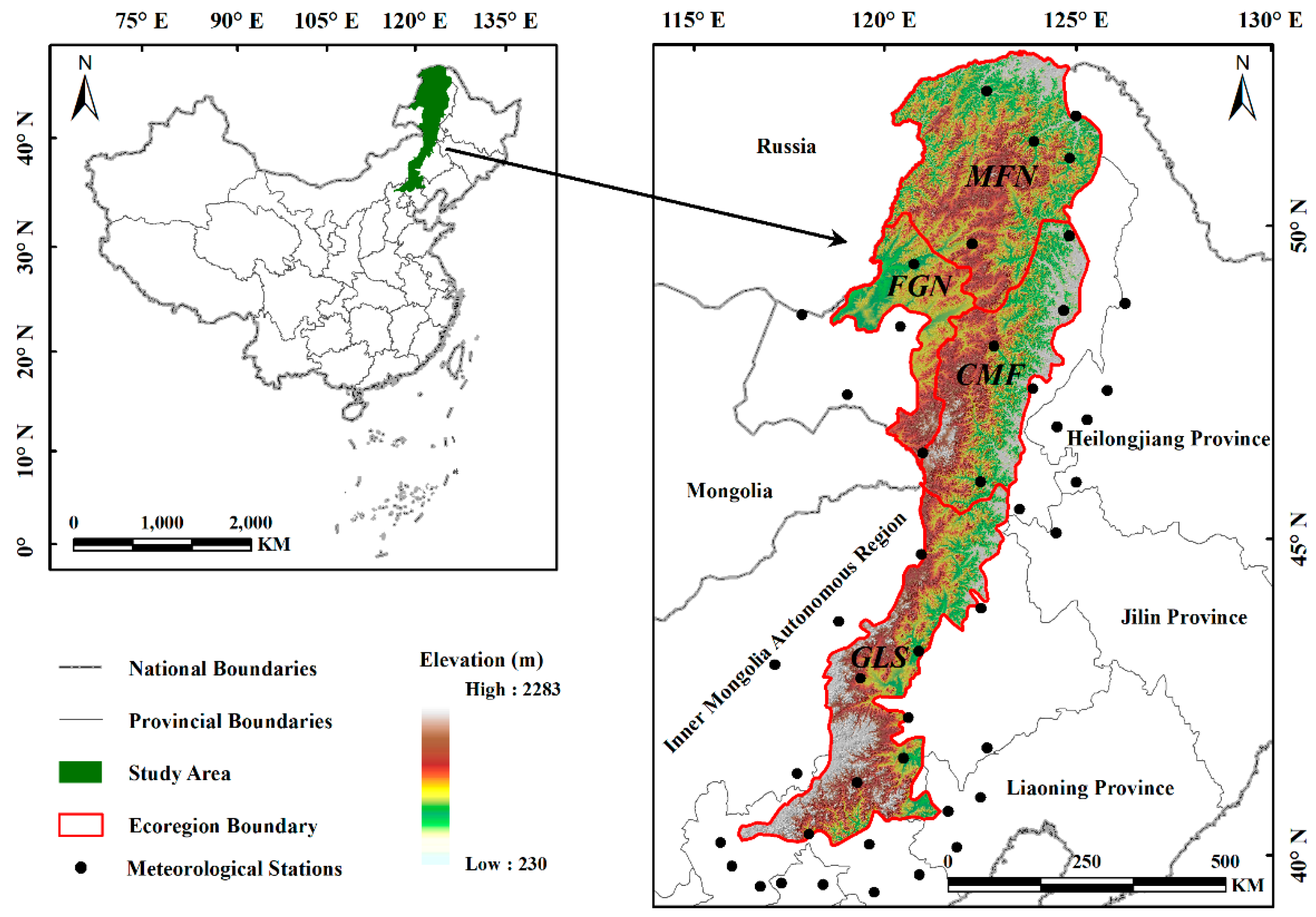
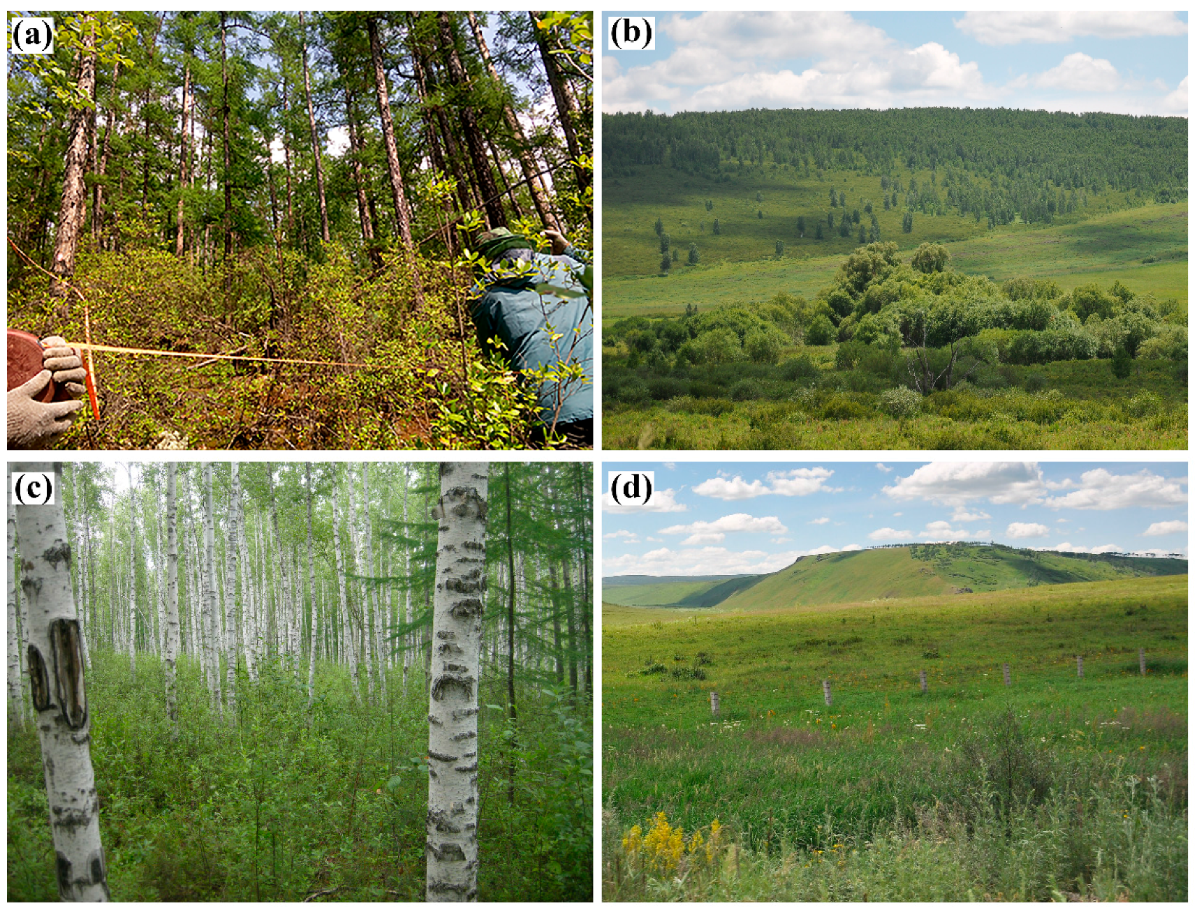
2.1. Study Area

The Greater Khingan Mountains (40°59′–53°33′N, 115°05′–125°16′E), China, are located in the eastern portion of the Inner Mongolia Autonomous Region, north of Heilongjiang Province, with a northeast–southwest orientation (Figure 1). The eastern and western slopes of this region are asymmetric; the terrain of the east facing slopes is steep, quickly incising to the Songliao Plain, whereas the terrain of the west facing slopes is relatively gentle, gradually transiting into the Mongolian Plateau. The Greater Khingan Mountains are an important climate demarcation line in China, with a decreasing temperature gradient (mid-temperate to cold temperate) from north to south and a decreasing humidity gradient (humid to semi-arid) from east to west. The summer marine monsoon is blocked by the east slope of the mountains, thus forming a precipitation contrast between the wetter eastern slopes and the arid western slopes. The variety of vegetation types in this region is abundant, with significant differences in vegetation composition among different regions. Cold–temperate coniferous forest cover is prevalent in the high-latitude regions, gradually transitioning to mid-temperate grassland landscapes with decreasing latitude.
The Greater Khingan Mountains are divided into four ecogeographical regions [26] according to the ecogeographical regionalization system of China, which reflects the regional differences of natural elements such as temperature, moisture, and vegetation cover (Figure 1 and Figure 2, Table 1): (i) the mountain deciduous coniferous forest region in the north (MFN); (ii) the forest grassland region in the northwest (FGN); (iii) the centrally located mountain grassland forest (CMF); (iv) and the grassland region in the south (GLS).

2.2. GIMMS NDVI3g Dataset

Since it can accurately represent vegetation growth status from different remote sensing information sources, NDVI is a commonly used indicator for monitoring vegetation phenology [28]. The third-generation NDVI (NDVI3g) used in this study is the latest and longest production of satellite NDVI records released by the Global Inventory Modeling and Mapping Studies (GIMMS) group [21]. It contains over 30 years of observations of 15-day maximum value compositions (MVC) at a spatial resolution of 8 km, and can be acquired from the NASA Ames Ecological Forecasting Lab (http://ecocast.arc.nasa.gov/data/pub/gimms/3g.v0/). Multiple corrections have been applied to eliminate errors and noise caused by satellite sensors, radiation, geometry, atmosphere, and other factors [22]. So, compared to the older versions, this dataset can provide higher quality data for regions in mid to high latitudes. In this study, we extracted the GIMMS NDVI3g pixels covering complete 34 years (January 1982–December 2015) to produce the NDVI time-series curve and derive phenological metrics.

2.3. Climate Data

Daily mean temperature and cumulative precipitation at 839 meteorological stations distributed throughout China from 1982 to 2015 were acquired from the China Meteorological Data Sharing Service System (http://cdc.cma.gov.cn). The daily climate data were compiled into monthly data, and then the stations based monthly climate data were interpolated into 8 km × 8 km grids to match the GIMMS NDVI3g dataset using ANUSPLIN 4.3. Finally, the gridded monthly temperature and precipitation data with spatial resolution 8 km × 8 km of the Greater Khingan Mountains from 1982 to 2015 were extracted by mask analysis.
The ANUSPLIN 4.3 algorithm applies a thin-plate spline function for interpolating meteorological data. Using this approach, a number of impact factors are used as covariates for spatially interpolating meteorological elements, greatly improving interpolation precision, and multiple surfaces can be interpolated simultaneously [29]. The program is particularly suited to interpolating time series meteorological data and has been widely applied in recent phenological research [30]. The measures of interpolation accuracy generated in the log file include the root of the generalized cross-validation (RTGCV), the root of the mean square error (RTMSE), the root of the mean square residual (RTMSR), and signal value. The signal value gives an indication of the degrees of freedom of the fitted spline. The best model judgment criteria [29] are the values of RTGCV, RTMSE, RTMSR, which are minimal, and the signal value, which is less than half the number of meteorological stations. In this study, we used the latitude, longitude, and monthly temperature or precipitation of each meteorological station as independent variables. Elevation, which is known to have a strong influence on climate [31], was a covariate incorporated into the interpolation process. Then, by comparing three test schemes (the number of splines was two, three, and four, respectively) based on the best model judgment criteria, we finally determined the second scheme as optimal to interpolate climate data. Elevations for this study were based on a resampled 8 km grid derived from a 90 m resolution digital elevation model (DEM) from the NASA and National Imagery and Mapping Agency (NIMA) Shuttle Radar Topography Mission (SRTM) (http://glcf.umd.edu/data/srtm/).

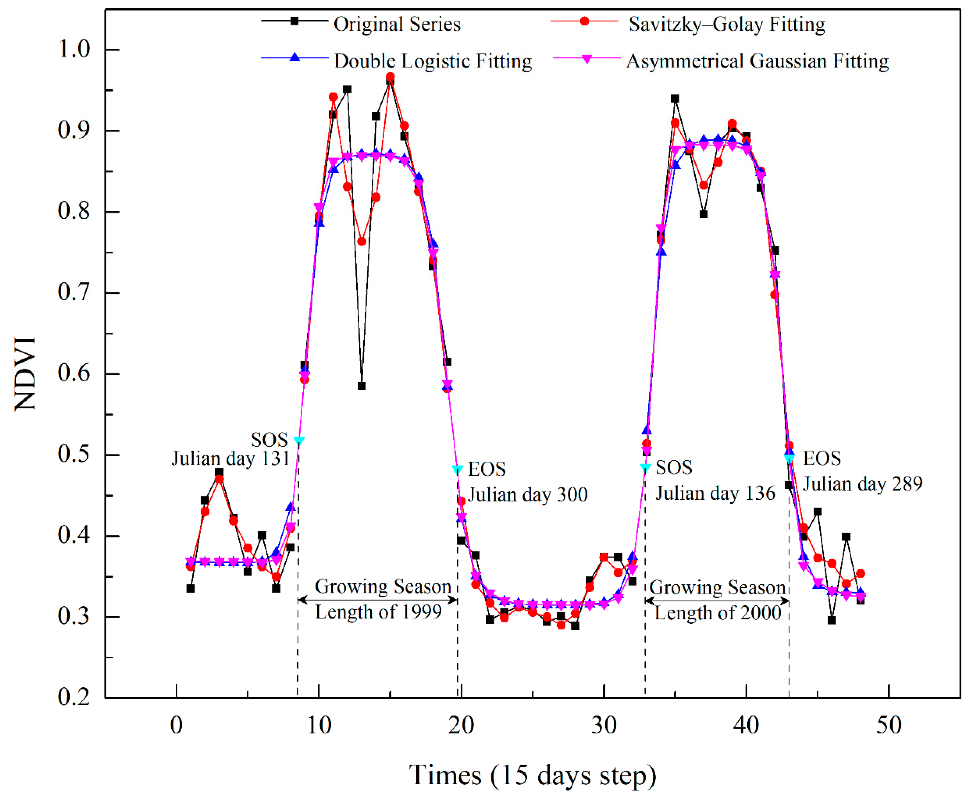
2.4. SOS and EOS Extraction

There is usually snow cover on the Greater Khingan Mountains from late autumn to the following late spring [32]. Snow cover would reduce the NDVI value of the land surface and misrepresent the photosynthetic capacity of vegetation during the non-growing season, which can lead to errors in extraction of phenological parameters [33]. Therefore, snow-covered NDVI during non-growing season should be eliminated first. According to the preprocessing method that has been validated in precious studies [20], we replaced the NDVI values of the pixels covered by snow with the median value of the snow-free winter NDVI values between November and the following March. Subsequently, we smoothed and reconstructed the NDVI time series by removing abnormal (extreme high/low) values, which were present due to atmospheric interference and sensor errors. Three time series reconstruction algorithms in the TIMESAT software [34] were tested to smooth and reconstruct the NDVI time series. These were Savitzky–Golay filtering (S–G), the double logistic function (DL), and the asymmetrical Gaussian function (AG). Since each of these aforementioned methods presents unique advantages and disadvantages, each was tested for the study area in order to choose the most appropriate algorithm. We randomly selected the samples in the study area, and the NDVI time series were fitted by the S–G, DL, and AG methods.
A comparison of the original and fitted curves of the GIMMS NDVI3g data at 15-day intervals (Figure 3) indicated that the S–G filtering approach yielded the closest match to the original data. However, the fitted curve of S–G had great volatility and was not smooth enough compared to the other two methods. A smoothed curve is more desirable as it prevents NDVI values from varying directionally over short intervals, and is thus more representative of actual annual vegetation growth. The DL and AG methods both produced smoothed curves with considerable noise reduction, while the performance of the two methods was similar and it was difficult to judge which was better. Therefore, we used three statistical indicators to evaluate the performance of DL and AG methods: (1) the root mean square error (RMSE); (2) Akaike’s Information Criterion (AIC); and (3) Bayesian Information Criterion (BIC). The number of free parameters of each method was the same as Atkinson et al. [35]. For the DL and AG methods, six and seven parameters were needed, respectively. The RMSE and AIC of AG method were both smaller than the values of DL method (Table 2). Thus, the AG method performed better than DL method. In addition, the AG function can generate a reconstructed NDVI curve that better describes subtle changes in the NDVI sequence data [36], more accurately reflects the characteristics of vegetation growth, and reduces the influence of outside interference factors (e.g., fire and pests). Therefore, the AG method was chosen as the time series reconstruction function to be used in this study.
After reconstructing the NDVI time series, the next step is to extract specific phenological parameters such as SOS and EOS. The most common methods for this step include the maximum slope method, the inflection-based method, and the dynamic threshold method. The maximum slope method defined SOS or EOS as the day of year (DOY) when NDVI begins to either rapidly increase (SOS) or decrease (EOS) [37], identified based on the maximum absolute slope of the fitted NDVI curve during growth or senescence [38]. The inflection-based method is an algorithm detecting points where maximum curvature occurs in a fitted NDVI time series [39]. SOS was defined as a valley point at the beginning of a growing cycle, and EOS was defined as a valley point at the decaying end of a phenology cycle [39]. The dynamic threshold method defines SOS and EOS as the DOY when the NDVIratio reaches a predefined threshold of the vegetation growth amplitude during the NDVI rising stage and decline stage, respectively [38]. However, the setting of thresholds is based on the characteristics of the NDVI curve, and these characteristics vary among vegetation types [40]. In addition, the extent of the study area is large and the type of vegetation is abundant. Therefore, in this study, different NDVI thresholds (e.g., 20%, 30%, 35%, 40%, 45%, or 50%) of multiple sampling sites in the study area were repeatedly tested. By comparison, we found that the extracted phenological parameters at the threshold of 30% were most consistent with the results of previous studies in similar areas [41,42]. Finally, we applied 30% as the dynamic threshold, which was also widely used for satellite-based phenology detection in previous studies [41,43] to extract EOS. The NDVIratio is defined as:
N D V I r a t i o = N D V I t N D V I m i n N D V I m a x N D V I m i n ,
where NDVIt is the NDVI value at time t; NDVImax represents the annual maximum NDVI value; for SOS, NDVImin represents the annual minimum NDVI value during the growth period; and for EOS, NDVImin represents the annual minimum NDVI value during the senescence period.
We applied the above three methods to extract the multiyear averaged EOS in the Greater Khingan Mountains. By comparison, we found the spatial patterns of the average EOS varied with different methods (Figure 4). The average EOS based on maximum slope method was earliest, ranging from Julian day 252 to 291. The average EOS based on dynamic threshold method occurred between Julian days 284 and 331, while the average EOS based on the inflection-based method was the latest, ranging from Julian day 288 to 354. The above results were similar to those of previous studies. You et al. [40] founded that the maximum slope method tended to estimate the EOS date earlier by comparing with the threshold and curvature change rate methods; Shang et al. [44] revealed that the inflection-based approach would overestimate the EOS when the vegetation was affected by disturbances, whereas the dynamic threshold approach can estimate it correctly. Additionally, the slope of vegetation NDVI curve was easily affected by external conditions, so the vegetation growth period could not be determined correctly based on the slope, which rendered the maximum slope method unsuitable for the extraction of phenological parameters of long time series [43]. Studies also showed that if some vegetation growth trajectories cannot be fitted well with a logistic function, it will prevent an inflection point from being determined correctly [45]. The vegetation growth curve of this study was fitted well by an AG function rather than a DL function, so the inflection-based method is not suitable for extracting the phenological parameters in our study area. Comparative studies [46] concluded that the dynamic threshold method is one of the simplest and most effective methods to extract phenological parameters, as it generally keeps dates within a reasonable range based on the threshold conditions and could achieve relatively high accuracy [40]. Moreover, compared with the other two methods, the range of the multiyear averaged EOS extracted from the threshold method was the most reasonable referring to the results of previous studies in similar areas. Thus, we finally used the dynamic threshold method to estimate the SOS and EOS over the Greater Khingan Mountains.

2.5. Investigating Trends in EOS, SOS, and Climatic Factors

We used Sen’s slope estimator to investigate temporal trends in EOS, SOS, and preseason climatic factors across the Greater Khingan Mountains from 1982 to 2015 at the pixel level, along with the Mann–Kendall trend test to determine their significance at each pixel. Compared with the linear trend based on the least squares method, Sen’s slope estimator can help diminish the influence of missing time series observations and non-normally distributed data on the analysis results, as well as reduce the interference of abnormal values in a time series [47]. Thus, this method is often used to analyze long-term sequence datasets to detect the magnitude of the trend:
Q = m e d i a n ( x j x i j i )   1 i < j n ,
where Q is the Sen’s slope; x j and x i represent the sequence value at time j and i, respectively; and median is calculated from all pairs of observations in the time series.
The Mann–Kendall trend test is one of the most common methods used for testing time series trends [48]. It does not require samples to follow a certain distribution, is not subject to the interference of a few extreme values, is suitable for hydrological, meteorological, and other non-normally distributed data, and has been widely used in the analysis of remotely-sensed data [47]. The combined use of Sen’s slope estimator and the Mann–Kendall trend test has become an important method for analyzing time series vegetation data [49].

2.6. Detecting the Correlation between EOS and SOS as Well as Climatic Factors

During multivariate correlation analysis, the influence of each variable is mutual. Therefore, the correlation between variables will not be truly reflected when correlation analysis is conducted using only two variables [15]. So, when analyzing the correlation between the two variables, the influence of other variables must be considered. To address this problem, we applied a temporal partial correlation analysis between EOS and SOS, and the preseason climatic factors. This approach was aimed at statistically investigating the relationship between EOS and a single driving factor while controlling the influence of the two remaining factors. This method has been commonly applied in climate change and ecological studies [3]. The partial correlation coefficients were also calculated for each ecogeographical region as well as the entire study area.

2.7. Determination of the Preseason

The preseason was defined as the period (with a one-month time-step) before the EOS date for which the correlation between EOS and climatic factors (e.g., temperature and precipitation) was highest during 1982–2015. Following previous studies, the maximum range of this period was set from May to the multiyear average date of EOS [50]. The average onset date of vegetation dormancy in the Greater Khingan Mountains over all pixels and years is around late October (as shown in Section 3), so the preseason in this study was defined as May through October.

3. Results

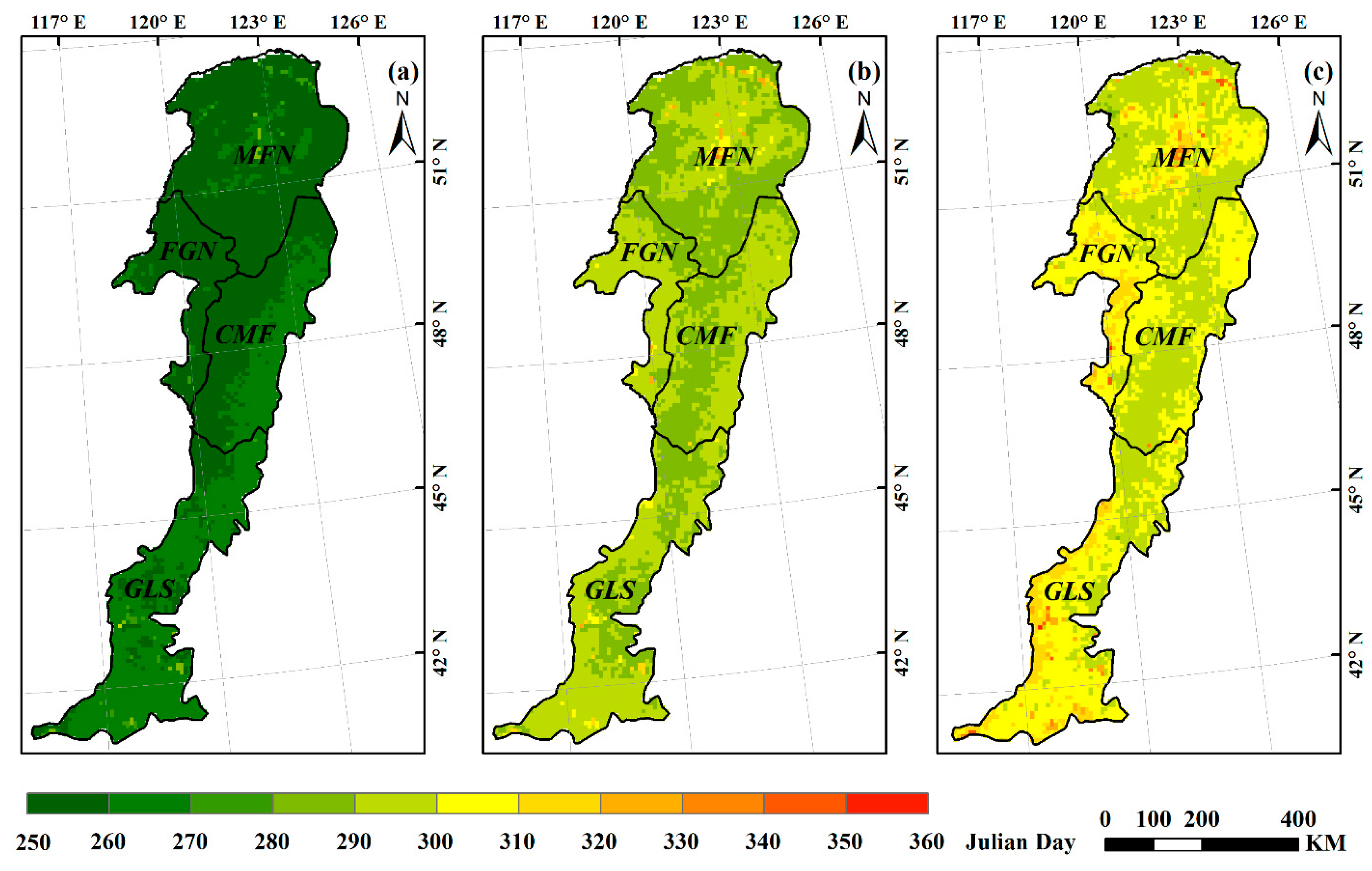
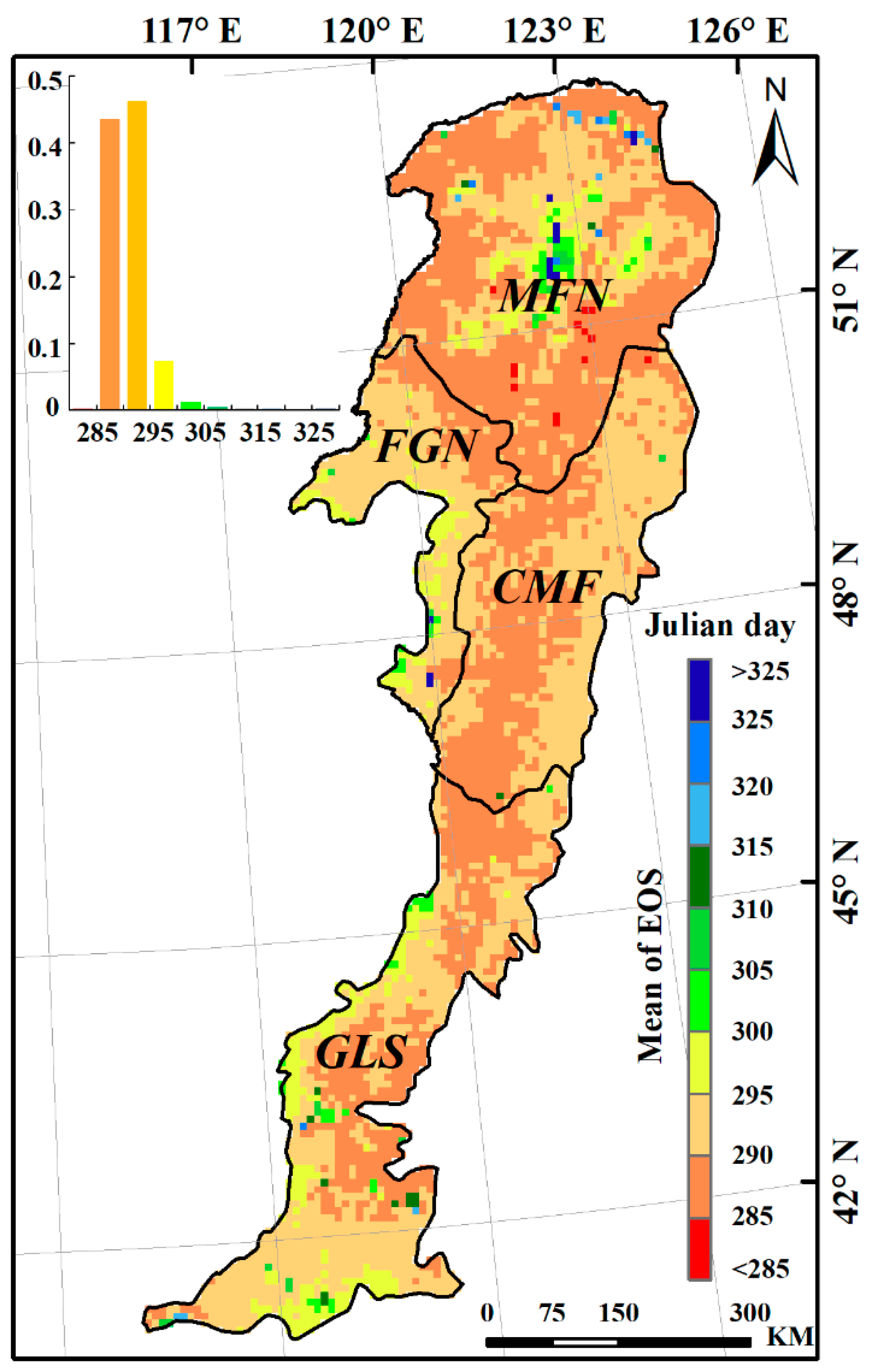
3.1. Spatial Pattern of Autumn Phenology

The average EOS dates during the study period (1982–2015) ranged from Julian day 284 to 331, with an average date of Julian day 292 (late October) for the study area (Figure 5). EOS dates at more than 90% of pixels occurred in October, from Julian day 285 through 305. Both the earliest and latest EOS dates were observed in the MFN region, with a difference of 47 days between them. The CMF region had the earliest EOS date, which occurred on Julian day 290 on average. The average EOS dates for the GLS and FGN regions were Julian days 291 and 292, respectively, slightly later than that observed in the CMF region.

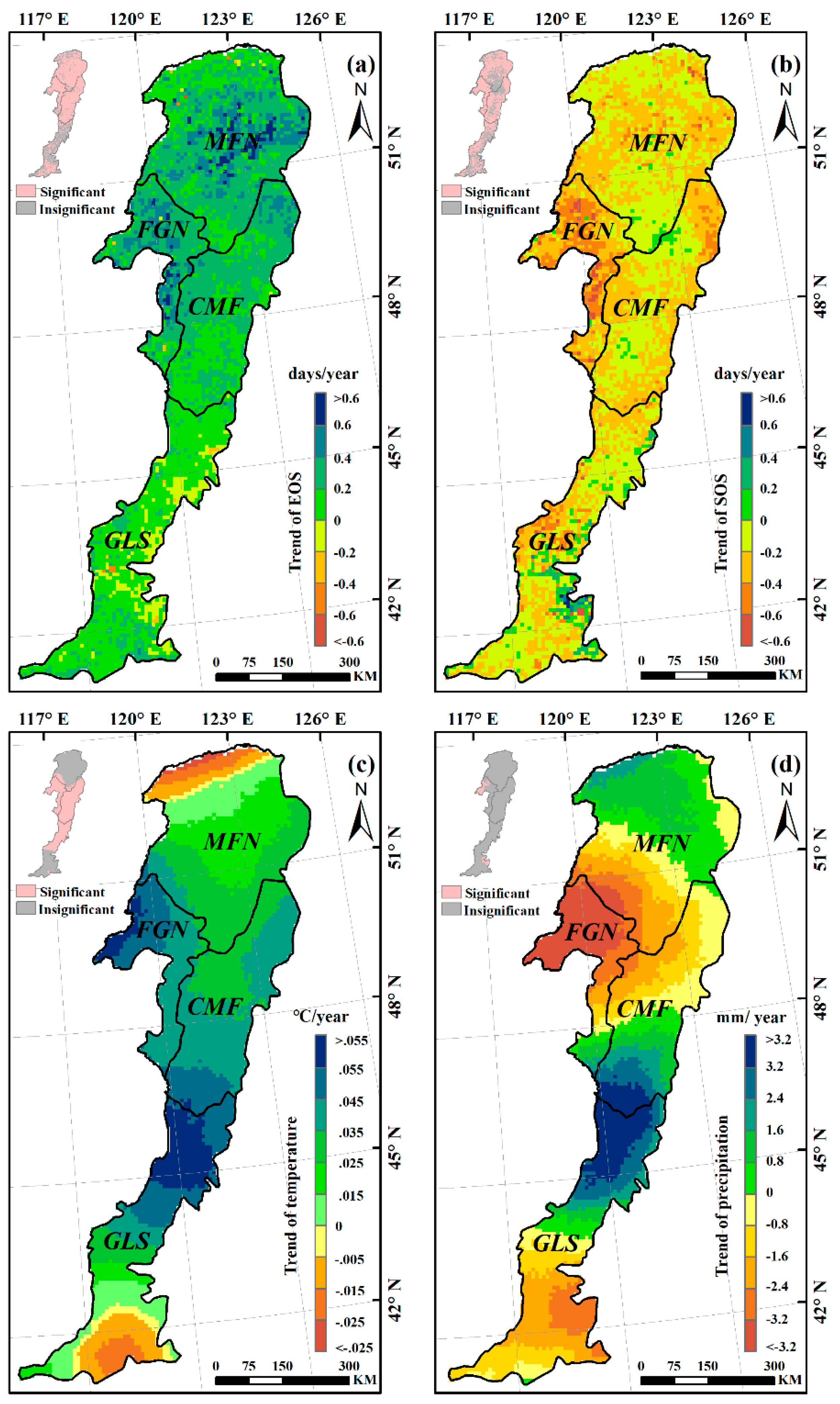
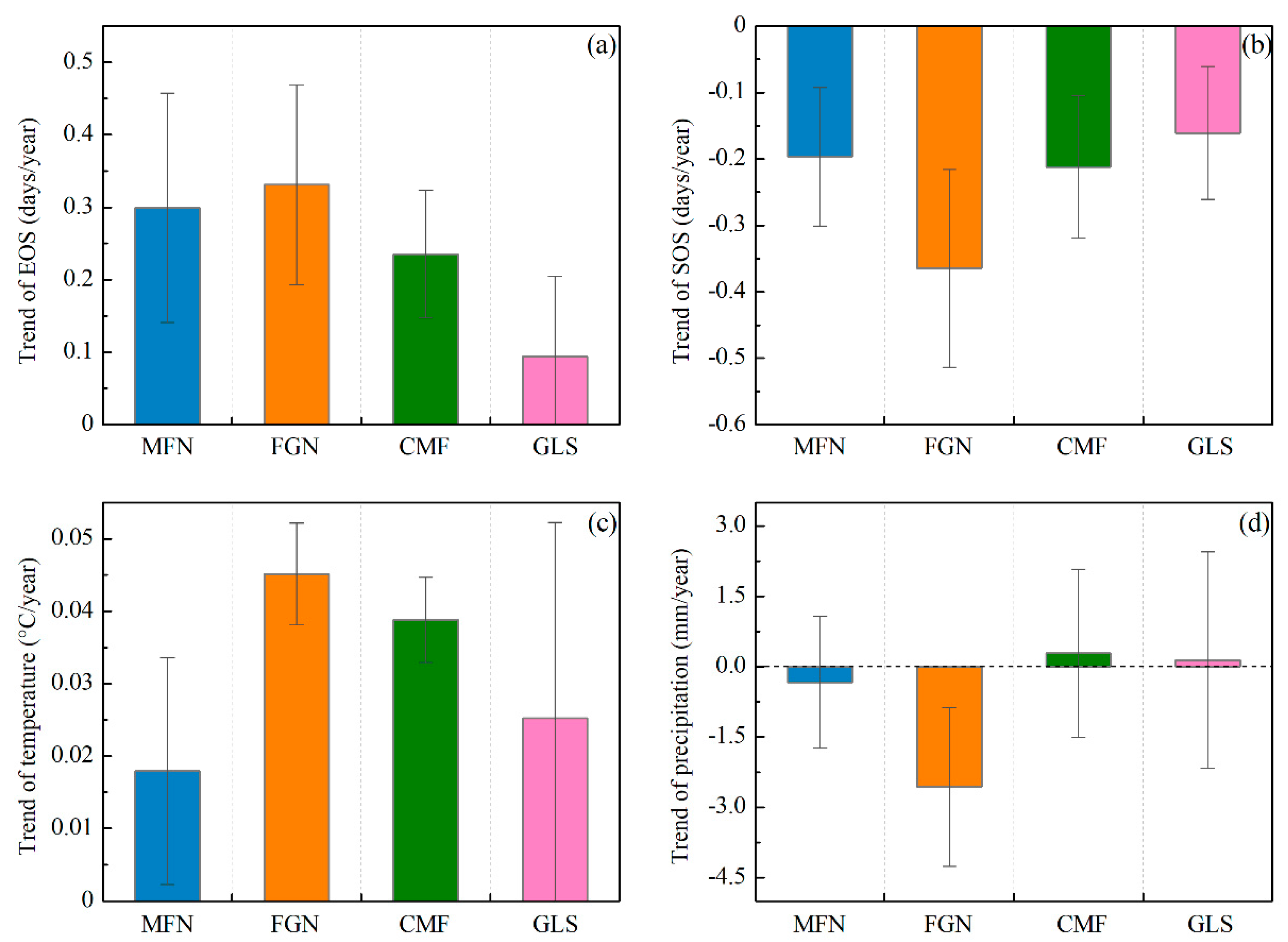
3.2. Trends in Autumn Phenology and Climatic Factors

The trends of the EOS, SOS, preseason temperature, and preseason precipitation were calculated at the 95% confidence level (Figure 6).The mean EOS date in the whole Greater Khingan Mountains had been delayed by 7.82 days over the past 34 years (an average rate of 0.23 days/y). More than 94% of the study area exhibited delayed trends of EOS, with roughly 72% showing significant delays (p < 0.05) (Figure 6a). The other ~6% of pixels showed earlier EOS, mainly in the southeastern of the study area, but only 12% were significant (p < 0.05). The mean EOS date of all the ecogeographical regions uniformly exhibited delayed trends. In the semi-arid GLS region, the mean EOS date exhibited a minimum delay of 3.06 days (0.09 days/y), while the mean EOS date of FGN region exhibited a maximum delay of 11.56 days (0.34 days/y) (Figure 7a).
During 1982–2015, a preseason temperature increase was observed in more than 88% of the study area (around 61% was statistically significant at p < 0.05), and occurred mainly in the FGN and CMF regions (Figure 6c). The preseason temperature in all of the ecogeographical regions (MFN, FGN, CMF, and GLS) exhibited a clear increasing trend (+0.02 °C/y, +0.05 °C/y, +0.04 °C/y, and +0.03 °C/y, respectively) (Figure 7c). For the spatial distribution of preseason precipitation variation, neither negative nor positive trends (both nearly 50%) dominated the entire study area (Figure 6d). In addition, the variation trends of preseason precipitation in all the ecogeographical regions were different. In the MFN and FGN regions, the preseason precipitation exhibited decreasing trends (−0.33mm/y and −2.6 mm/y, respectively), while in the CMF and GLS regions, the preseason precipitation exhibited increasing trends (+0.29 mm/y and +0.15 mm/y, respectively) (Figure 7d).

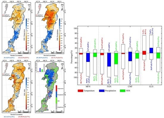
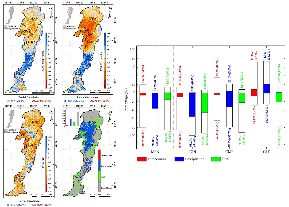
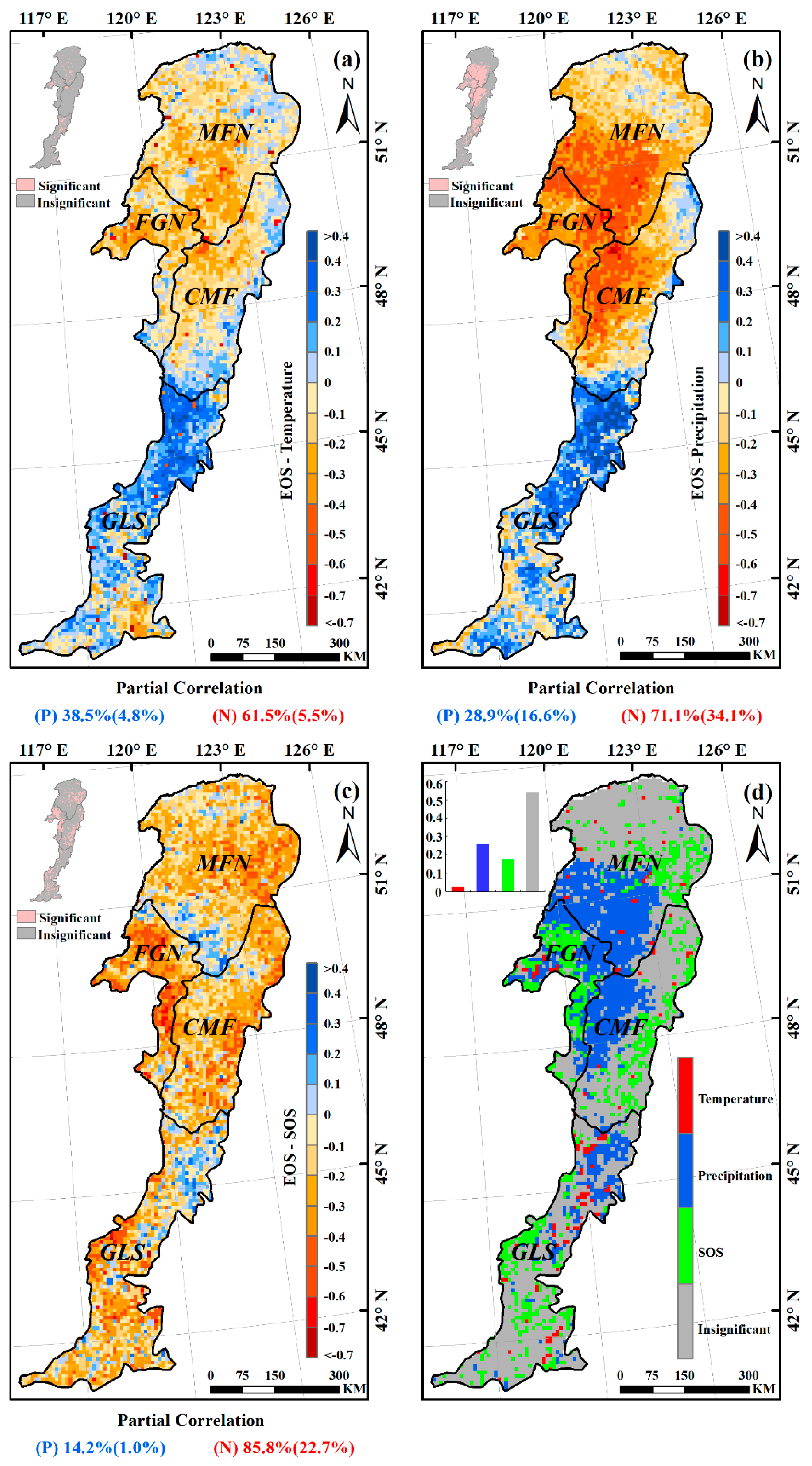
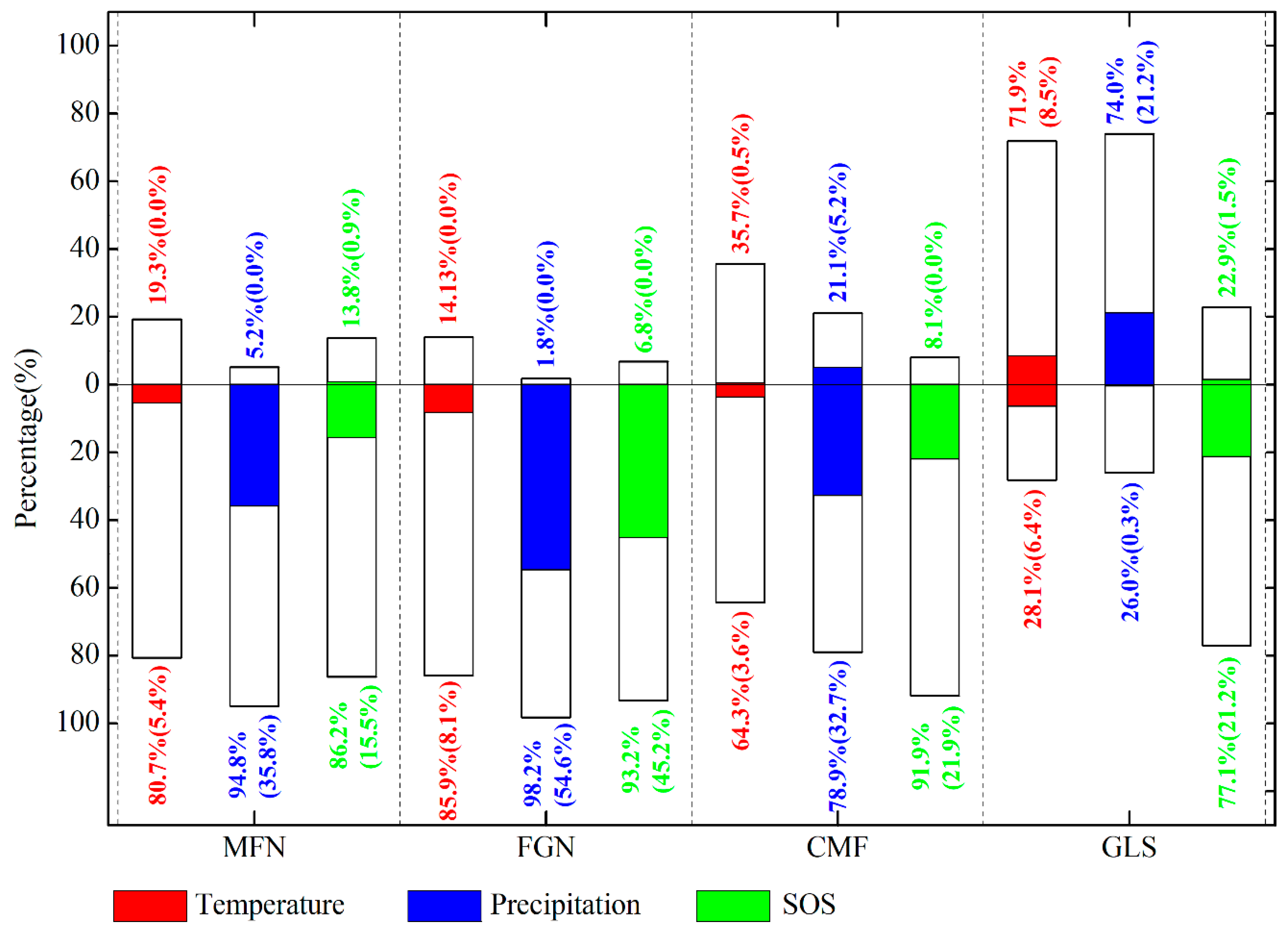
3.3. Effects of Climatic Factors on Autumn Phenology

The partial correlation coefficients between EOS and preseason temperature, preseason precipitation, SOS were also calculated at 95% confidence level (Figure 8). Over 61% of the entire study area showed negative partial correlations between preseason temperature and EOS (about 6% of the relationships were significant at p < 0.05), the remaining ~38% of the study area showed positive partial correlations (Figure 8a). In the humid and semi-humid regions (MFN, FGN, and CMF), more than 60% of each presented negative partial correlations between preseason temperature and EOS (Figure 9), suggesting that higher temperature during the preseason led to an earlier EOS in most of these areas. In most of the semi-arid GLS region, however, increased preseason temperature played a role in delaying the EOS date (about 72% of this region exhibited positive partial correlations) (Figure 9).
Negative partial correlations between preseason precipitation and EOS dominated about 71% of the study area, and about 34% of them were significant (p < 0.05), indicating that increased precipitation during preseason would advance the EOS date (Figure 8b). Interestingly, in each of all the four ecogeographical regions, the relationships between preseason precipitation and EOS were same as that between preseason temperature and EOS (Figure 9). In the humid and semi-humid regions (MFN, FGN, and CMF), most of each region (94%, 98%, and 78%, respectively) experienced negative partial correlations between preseason precipitation and EOS. While in 74% of semi-arid GLS region, the partial correlations were positive, suggesting that increasing precipitation during the preseason could contribute to the extension of EOS.

3.4. Relationship between Spring Phenology and Autumn Phenology

Contrary to the delayed trend observed for EOS change, the mean date of the SOS in the Greater Khingan Mountains advanced an average of 0.20 days/y from 1982 to 2015. More than 94% of the pixels exhibited earlier trends of SOS, with more than 65% significant (p < 0.05) (Figure 6b). In addition, in each of the four ecogeographical regions, the mean SOS date all exhibited an earlier trend over the past 34 years (Figure 7b).
Negative partial correlations between EOS and SOS dominated the whole study area (more than 85%), with more than 22% of pixels having statistically significant relationships between the two variables (p < 0.05). Positive partial correlations were observed primarily in the southern MFN and northern GLS regions (Figure 8c). In each of the four ecogeographical regions, SOS was negatively associated with EOS. This was especially true in the FGN region, over 93% of which was absolutely dominated by negative relationships, with more than 45% statistically significant (p < 0.05) (Figure 9).

3.5. Spatial Pattern of the Dominant Factors Affecting Autumn Phenology

Preseason precipitation was the main driver of interannual EOS variations for 26% of all pixels, followed by SOS (17%), and preseason temperature (3%) (Figure 8d). The remaining pixels were not statistically significant at the p < 0.05 level. Preseason precipitation was the primary determinant of the EOS changes in the southwestern MFN, northeastern FGN, and western CMF regions. Preseason temperature sporadically controlled the EOS changes of a small number of pixels, however, indicating that precipitation was the main climatic driver of EOS changes in most of the Greater Khingan Mountains during the preseason. Additionally, SOS showed a certain driving effect on the EOS changes.

4. Discussion

4.1. Relationship between Autumn Phenology and Climatic Factors

Our results indicated that the average EOS date in the Greater Khingan Mountains, northeastern China during 1982–2015 had a delayed trend of 0.23 days/y, generally consistent with the results of previous studies also showing a delayed EOS trend in the Northern Hemisphere [9], Europe [51], North America [52], and temperate China [50]. Zhao et al. [41] estimated the EOS across the entire Northeast China from 1982 to 2013 and found a delay of 0.13 days/y. Tang et al. [42] reported EOS changes in the Hulunber of northeastern China during 1982–2012, with an average delay of 0.29 days/y. Compared to the two above studies investigating the similar study area (northeastern China) and using the same data source (GIMMS NDVI3g), the delayed rate of EOS observed in this study was slightly different from the results of these studies, possibly because the specific location of study area and the phenology extraction method were different. However, the comparison showed that the results of our study could explain well the change of autumn phenology in the Greater Khingan Mountains.
The terrain of the Greater Khingan Mountains is complex and climatic conditions vary across the region. Thus, the response of the EOS to climatic changes varied by latitude. We found that preseason temperature was generally negatively correlated with the EOS date in the MFN, FGN, and CMF regions. For the MFN and CMF regions, which are mainly covered in deciduous trees, this finding may be due to warming-induced enhancement of tree canopy transpiration, in which the roots of trees lacked moisture, thus reducing water utilization [53] and subsequently leading to earlier EOS. In addition, because permafrost is present in portions of these two regions, trees growth, especially the formation and development of Larix gmelini forest, was closely related to the alpine and permafrost environment [54]. Permafrost could provide the needed moisture for tree growth, whereas high temperature would decrease the soil freezing depth and the protection of the aquifers, weaken the soil water retention, and thus in the dry season prevent adequate water for trees growth, accelerating leaf senescence [55]. Another reason may be that leaves of deciduous trees need a certain accumulated temperature from growth to senescence, and preseason temperature increase makes the tree leaves obtain the required accumulated temperature in a short period of time, thus leading to earlier wilting dates [56]. For the FGN region, which is dominated by herbaceous plants (Stipa baicalensis meadow steppe, Filifolium sibiricum meadow steppe), warmer temperatures during the preseason would also accelerate the end of the growing season. This may be because the preseason temperature in this region exhibited the most significant increasing trend (Figure 7c). Thus, an excessive increase in preseason temperature will limit vegetation growth in this region [57]. Similarly, preseason precipitation was also negatively correlated with the EOS in most of the MFN, FGN, and CMF regions. The reason may be that the MFN, FGN, and CMF regions are located in humid and semi-humid areas with rain and heat over the same period and abundant rainfall. Soil moisture will rapidly increase with the increasing precipitation during the preseason, and then enhance the vegetation photosynthesis by affecting the vegetation carboxylation. The vegetation will accelerate growth and complete the entire growing season ahead of schedule [58]. Additionally, due to the impact of permafrost, high soil moisture in these colder areas may limit the availability of nutrients for vegetation growth [59], thus prematurely ending vegetation growth.
In most of the grassland semi-arid region (GLS), which is mainly covered in herbaceous plants, a warming preseason temperature delayed the EOS date, which was consistent with findings in previous studies based on satellite data and field experiments [60]. This result is probably because warming in summer and autumn can enhance the activities of photosynthetic enzymes [61], reduce the rate of chlorophyll degradation during leaf senescence in autumn, and thus delay the time of leaf senescence [62]. Furthermore, herbaceous plants are more sensitive to chilling injury compared to deciduous trees, so the warmer preseason may increase the number of days available for vegetation growth and photosynthesis [63], reduce the probability of frost damage [64], and thereby postpone the autumn phenology of herbaceous plants in the GLS region. Positive effects of preseason precipitation on the EOS date of GLS region were also revealed in this study. Possibly due to shallow roots, herbaceous plants in semi-arid region are often subjected to water stress, and their growth is bound to respond rapidly to water. Increasing precipitation during the preseason can effectively alleviate water stress, thus delaying the EOS date and prolonging the growing season [65]. In summary, preseason precipitation had a greater impact than temperature on the EOS in most of the Greater Khingan Mountains. Climate change has a direct impact on vegetation phenology and also indirectly affects ecological processes such as species competitive balance, which may alter forest composition (e.g., proportions of coniferous vs. deciduous), which ultimately affects phenological change [66]. Previous studies [67] showed that temperature increase may result in the area of coniferous species contracted and broadleaf species expanded, with potential to replace coniferous forest completely. However, tree species migration usually lags behind warming for decades or even a century [68]. Therefore, we believe over the past 34 years the impact of climate change on ecological processes may not greatly change forest composition and consequently may not alter our results on the phenological change in the Greater Khingan Mountains. Overall, the relationship between autumn phenology of different vegetation and climatic factors is complex and the impact mechanisms affecting delayed autumn phenology need to be further explored.

4.2. The Influence of Spring Phenology on Autumn Phenology

Our results showed that there was a strong positive correlation between SOS and EOS at the pixel level in the southwestern MFN and the northeastern GLS regions, suggesting that an earlier spring phenology would lead to an earlier autumn phenology. Many mechanistic studies have been conducted to explain this phenomenon. First, as the influencing factor of leaf traits, programmed cell death [69] and leaf longevity [70] were reported to constrain the timing of leaf senescence. Second, earlier springs may result in soil water losses via increases in snow sublimation and evapotranspiration in the early part of the growing season; thus, summer and autumn drought duration may increase, leading to earlier EOS dates [71]. Third, earlier spring budburst can increase the risk of vegetation suffering damage such as spring frost [72] and insect disease [73], thereby inducing earlier leaf senescence. Finally, the size of the vegetation carbon sink was also found to restrict the correlation between spring and autumn phenology because the accumulation of unstructured carbohydrates in earlier spring may contribute to an earlier peak in autumn carbon content [15]. Negative partial correlations between the SOS and EOS also occurred in the Greater Khingan Mountains; specifically, an earlier SOS was followed by a delayed EOS. This special situation may not be explained by the internal mechanism of vegetation alone. The SOS is also significantly affected by climatic factors, showing an earlier trend in other regions under the context of climate warming [4,28], which is consistent with our results.

4.3. Uncertainty

In general, there are six methods to reconstruct NDVI time series [18,35]. These are (1) Savitzky–Golay filter (S–G); (2) double logistic function (DL); (3) the asymmetric Gaussian function (AG); (4) the harmonic analysis of time series (HANTS); (5) the Fourier transform (FT); and (6) the innovative Whittaker smoother (WS). Each method has advantages and disadvantages, and there is no universal method suitable for all vegetation types of specific study areas [35]. The choice of the method depends on the purpose of the study. TIMESAT is a free software package for processing satellite time series data. The software can adapt to the upper envelope of the data, taking missing data and quality flags into account, and has been widely used in a large number of applied studies for data smoothing and phenology parameter extraction [34]. TIMESAT only has three models (S–G, DL, AG), so we only tested the S–G, DL, and AG models in this study. The parameter settings of S–G might be off the norm, and we adopted the settings from Zhao et al. [41] (an adaptation strength of 2.0, no spike filtering, a seasonal parameter of 0.5, a seasonal parameter of 0.5, a window size of 2). In this study, we did not take the other common smooth methods (e.g., HANTS, FT, WS) into account, especially the innovative Whittaker smoother, which fits a discrete series to discrete data and penalizes the roughness of the smooth curve, balances reliability of the data, and roughness of the fitted data and may produce a better resulting curve [74]. Thus, the finally selected AG method in this study may not be optimal, and a comprehensive comparison of these methods needs to be conducted.
The spatial resolution of GIMMS NDVI3g dataset used in our study was 8 km. Coarse spatial resolution (8 km) that caused mixed vegetation types was the main source of uncertainties. Each pixel value is the mean reflectance of several land cover types over an area of 64 km2. Consequently, the processed value approximated the phenology of the dominant vegetation type and overlooked the minor cover types, leading to uncertainties in capturing the phenology of all vegetation types [41]. However, our study was based on a regional scale, and researchers have used the NDVI3g dataset with 8 km spatial resolution for phenology study at regional to continental scales [9,42,50], which provided effective information on seasonal variation of vegetation phenology over a long time period and with continuous spatial coverage. Moreover, higher resolutions may not necessarily lead to more accurate results [75]. Studies showed that fusing multi-source remote sensing data with different spatial resolutions is considered a feasible way to reduce this uncertainty [76].
The curve of long time series remote sensing data (e.g., NDVI) reflected vegetation dynamics. When the vegetation is affected by disturbances (e.g., wind, pests, fire, and human activities) [77], aberrations would be found in the curve. Disturbances affect phenology in a stochastic manner, leading to another source of uncertainties. When large-scale phenological parameters are extracted, it is difficult to remove the influences of all disturbances during all the study years, thus the results of this study could also potentially be affected.
In addition, solar radiation [9], atmospheric CO2 concentrations [78], nutrient availability [6], and other factors could also affect autumn phenology. Especially solar radiation, as another important climate factor and a combination of both photoperiod and solar intensity, would trigger autumn phenology in mid–high latitudes [9]. Specifically, increased insolation can retard the accumulation of abscisic acid and subsequently slow down leaf senescence [79]. Furthermore, the chlorophyll levels of leaves will increase due to the enhanced photosynthetic capacity and CO2 sequestration caused by the increased insolation, and result in a delayed EOS date [80]. However, it is difficult to take all of these factors into consideration in a large-scale remote sensing application. The phenological remote sensing models used in the present studies only make use of time series remote sensing data (e.g., NDVI, EVI) to extract phenological parameters without incorporating other potential phenological restriction factors [9,41]. In addition, we only analyzed the effects of temperature and precipitation on autumn phenology in this study. Therefore, we should consider these factors as much as possible in follow-up studies to reduce uncertainties in the results.

5. Conclusions

In this study, we extracted phenological parameters for the Greater Khingan Mountains from 1982 to 2015 based on the GIMMS NDVI3g dataset and an asymmetric Gaussian fitting function. We analyzed the interannual variation and the influence of major environmental controls on the EOS. Results showed that the EOS in the entire Greater Khingan Mountains and each of its ecogeographical regions all exhibited a delayed trend over the past 34 years. Furthermore, the driving factor of the EOS varied among the different ecogeographical regions (MFN, FGN, CMF, and GLS regions). Both increasing temperature and precipitation during the preseason (May through October) accelerated leaf senescence in autumn at mid–high latitudes (MFN, FGN, and CMF regions), with the exception of the semi-arid region (GLS), where the warming temperature and increased precipitation in summer/autumn delayed the EOS. Importantly, the preseason precipitation was a stronger driver of EOS changes relative to preseason temperature. Apart from climatic factors, we found that the SOS also had effects on the EOS, with mainly negative correlations across most of the study area. However, in the southwestern MFN and northeastern GLS regions, an earlier SOS resulted in an earlier EOS. In addition, compared with climatic factors, SOS played a more significant role than preseason temperature. The results of our study provide a useful reference for understanding the interannual variation of autumn phenology in mid–high latitudes and its response to climate change. In addition, given the important role of autumn phenology in regulating the global carbon budget, our study suggests that both climatic factors and SOS should be assembled into the EOS models to more accurately simulate changes in autumn phenology.

Acknowledgments

This work was supported by the National Key Research and Development Project (Grant No. 2016YFA0602301), the National Natural Science Foundation of China (Grant No. 41771450, 41501449), the Fundamental Research Funds for the Central Universities (Grant No. 2412017FZ021) and the University of Missouri GIS Mission Enhancement Program.

Author Contributions

All authors made great contributions to the work. Specific contributions include data collection and image processing (Yuanyuan Fu, Hong S. He, Jianjun Zhao), data analysis and manuscript preparation (Yuanyuan Fu, Hong S. He, David R. Larsen), and methodological guidance and technical support (Hongyan Zhang, Michael G. Sunde, Shengwu Duan).

Conflicts of Interest

The authors declare no conflict of interest.

References

  1. Piao, S.; Ciais, P.; Friedlingstein, P.; Peylin, P.; Reichstein, M.; Luyssaert, S.; Margolis, H.; Fang, J.; Barr, A.; Chen, A. Net carbon dioxide losses of northern ecosystems in response to autumn warming. Nature 2008, 451, 49–52. [Google Scholar] [CrossRef] [PubMed]
  2. Wu, C.; Gonsamo, A.; Gough, C.M.; Chen, J.M.; Xu, S. Modeling growing season phenology in north american forests using seasonal mean vegetation indices from modis. Remote Sens. Environ. 2014, 147, 79–88. [Google Scholar] [CrossRef]
  3. Fu, Y.H.; Zhao, H.; Piao, S.; Peaucelle, M.; Peng, S.; Zhou, G.; Ciais, P.; Huang, M.; Menzel, A.; Peñuelas, J. Declining global warming effects on the phenology of spring leaf unfolding. Nature 2015, 526, 104–107. [Google Scholar] [CrossRef] [PubMed]
  4. Fu, Y.H.; Piao, S.; Op de Beeck, M.; Cong, N.; Zhao, H.; Zhang, Y.; Menzel, A.; Janssens, I.A. Recent spring phenology shifts in western central europe based on multiscale observations. Glob. Ecol. Biogeogr. 2014, 23, 1255–1263. [Google Scholar] [CrossRef]
  5. Gallinat, A.S.; Primack, R.B.; Wagner, D.L. Autumn, the neglected season in climate change research. Trends Ecol. Evol. 2015, 30, 169–176. [Google Scholar] [CrossRef] [PubMed]
  6. Estiarte, M.; Peñuelas, J. Alteration of the phenology of leaf senescence and fall in winter deciduous species by climate change: Effects on nutrient proficiency. Glob. Chang. Biol. 2015, 21, 1005–1017. [Google Scholar] [CrossRef] [PubMed]
  7. Zhu, W.; Tian, H.; Xu, X.; Pan, Y.; Chen, G.; Lin, W. Extension of the growing season due to delayed autumn over mid and high latitudes in north america during 1982–2006. Glob. Ecol. Biogeogr. 2012, 21, 260–271. [Google Scholar] [CrossRef]
  8. Garonna, I.; Jong, R.; Wit, A.J.; Mücher, C.A.; Schmid, B.; Schaepman, M.E. Strong contribution of autumn phenology to changes in satellite—Derived growing season length estimates across europe (1982–2011). Glob. Chang. Biol. 2014, 20, 3457–3470. [Google Scholar] [CrossRef] [PubMed]
  9. Liu, Q.; Fu, Y.H.; Zhu, Z.; Liu, Y.; Liu, Z.; Huang, M.; Janssens, I.A.; Piao, S. Delayed autumn phenology in the northern hemisphere is related to change in both climate and spring phenology. Glob. Chang. Biol. 2016, 22, 3702–3711. [Google Scholar] [CrossRef] [PubMed]
  10. Liu, Q.; Fu, Y.H.; Zeng, Z.; Huang, M.; Li, X.; Piao, S. Temperature, precipitation, and insolation effects on autumn vegetation phenology in temperate china. Glob. Chang. Biol. 2016, 22, 644–655. [Google Scholar] [CrossRef] [PubMed]
  11. Cong, N.; Shen, M.; Piao, S. Spatial variations in responses of vegetation autumn phenology to climate change on the tibetan plateau. J. Plant Ecol. 2016, 10, 744–752. [Google Scholar] [CrossRef]
  12. Xie, Y.; Wang, X.; Wilson, A.M.; Silander, J.A. Predicting autumn phenology: How deciduous tree species respond to weather stressors. Agric. For. Meteorol. 2018, 250, 127–137. [Google Scholar] [CrossRef]
  13. Rohde, A.; Bastien, C.; Boerjan, W. Temperature signals contribute to the timing of photoperiodic growth cessation and bud set in poplar. Tree Physiol. 2011, 31, 472–482. [Google Scholar] [CrossRef] [PubMed]
  14. Marchin, R.M.; Salk, C.F.; Hoffmann, W.A.; Dunn, R.R. Temperature alone does not explain phenological variation of diverse temperate plants under experimental warming. Glob. Chang. Biol. 2015, 21, 3138–3151. [Google Scholar] [CrossRef] [PubMed]
  15. Fu, Y.S.; Campioli, M.; Vitasse, Y.; De Boeck, H.J.; Van den Berge, J.; AbdElgawad, H.; Asard, H.; Piao, S.; Deckmyn, G.; Janssens, I.A. Variation in leaf flushing date influences autumnal senescence and next year’s flushing date in two temperate tree species. Proc. Natl. Acad. Sci. USA 2014, 111, 7355–7360. [Google Scholar] [CrossRef] [PubMed]
  16. White, M.A.; Beurs, D.; Kirsten, M.; Didan, K.; Inouye, D.W.; Richardson, A.D.; Jensen, O.P.; O’Keefe, J.; Zhang, G.; Nemani, R.R. Intercomparison, interpretation, and assessment of spring phenology in North America estimated from remote sensing for 1982–2006. Glob. Chang. Biol. 2009, 15, 2335–2359. [Google Scholar] [CrossRef]
  17. Xie, Y.; Sha, Z.; Yu, M. Remote sensing imagery in vegetation mapping: A review. J. Plant Ecol. 2008, 1, 9–23. [Google Scholar] [CrossRef]
  18. Geng, L.; Ma, M.; Wang, X.; Yu, W.; Jia, S.; Wang, H. Comparison of eight techniques for reconstructing multi-satellite sensor time-series ndvi data sets in the heihe river basin, China. Remote Sens. 2014, 6, 2024–2049. [Google Scholar] [CrossRef]
  19. Militino, A.F.; Ugarte, M.D.; Pérez-Goya, U. Stochastic spatio-temporal models for analysing ndvi distribution of gimms ndvi3g images. Remote Sens. 2017, 9, 76. [Google Scholar] [CrossRef]
  20. Shen, M.; Zhang, G.; Cong, N.; Wang, S.; Kong, W.; Piao, S. Increasing altitudinal gradient of spring vegetation phenology during the last decade on the qinghai–tibetan plateau. Agric. For. Meteorol. 2014, 189, 71–80. [Google Scholar] [CrossRef]
  21. Pinzon, J.E.; Tucker, C.J. A non-stationary 1981–2012 avhrr ndvi3g time series. Remote Sens. 2014, 6, 6929–6960. [Google Scholar] [CrossRef]
  22. Zhu, Z.; Bi, J.; Pan, Y.; Ganguly, S.; Anav, A.; Xu, L.; Samanta, A.; Piao, S.; Nemani, R.R.; Myneni, R.B. Global data sets of vegetation leaf area index (lai) 3g and fraction of photosynthetically active radiation (fpar) 3g derived from global inventory modeling and mapping studies (gimms) normalized difference vegetation index (ndvi3g) for the period 1981 to 2011. Remote Sens. 2013, 5, 927–948. [Google Scholar]
  23. Chen, X.; Hu, B.; Yu, R. Spatial and temporal variation of phenological growing season and climate change impacts in temperate eastern china. Glob. Chang. Biol. 2005, 11, 1118–1130. [Google Scholar] [CrossRef]
  24. Piao, S.; Fang, J.; Zhou, L.; Ciais, P.; Zhu, B. Variations in satellite-derived phenology in china’s temperate vegetation. Glob. Chang. Biol. 2006, 12, 672–685. [Google Scholar] [CrossRef]
  25. Cane, M.A. Climate science: Decadal predictions in demand. Nat. Geosci. 2010, 3, 231–232. [Google Scholar] [CrossRef]
  26. Zheng, D.; Yang, Q.; Wu, S.; Li, B. The Systematic Research of Chinese Eco-Geographical Area, 1st ed.; The Commercial Press: Beijing, China, 2008. [Google Scholar]
  27. Liu, X.; Jin, X.; Ke, C. Accuracy evaluation of the ims snow and ice products in stable snow covers regions in china. J. Glaciol. Geocryol. 2014, 36, 500–507. [Google Scholar]
  28. Zhao, J.; Zhang, H.; Zhang, Z.; Guo, X.; Li, X.; Chen, C. Spatial and temporal changes in vegetation phenology at middle and high latitudes of the northern hemisphere over the past three decades. Remote Sens. 2015, 7, 10973–10995. [Google Scholar] [CrossRef]
  29. Hutchinson, M.F.; Xu, T. Anusplin Version 4.3 User Guide; Centre for Resource and Environmental Studies, The Australian National University: Canberra, Australia, 2004. [Google Scholar]
  30. Dong, T.; Liu, J.; Shang, J.; Qian, B.; Huffman, T.; Zhang, Y.; Champagne, C.; Daneshfar, B. Assessing the impact of climate variability on cropland productivity in the canadian prairies using time series modis fapar. Remote Sens. 2016, 8, 281. [Google Scholar] [CrossRef]
  31. Pauchard, A.; Milbau, A.; Albihn, A.; Alexander, J.; Burgess, T.; Daehler, C.; Englund, G.; Essl, F.; Evengård, B.; Greenwood, G.B. Non-native and native organisms moving into high elevation and high latitude ecosystems in an era of climate change: New challenges for ecology and conservation. Biol. Invasions 2016, 18, 345–353. [Google Scholar] [CrossRef]
  32. Zhao, X.-M.; Li, D.-L.; Chen, G.-Y. Gis-based spatializing method for estimating snow cover depth in northeast china and its nabes. Arid Zone Res. 2012, 29, 927–933. [Google Scholar]
  33. Shen, M.; Sun, Z.; Wang, S.; Zhang, G.; Kong, W.; Chen, A.; Piao, S. No evidence of continuously advanced green-up dates in the tibetan plateau over the last decade. Proc. Natl. Acad. Sci. USA 2013, 110, E2329. [Google Scholar] [CrossRef] [PubMed]
  34. Eklundh, L.; Jönsson, P. Timesat: A software package for time-series processing and assessment of vegetation dynamics. In Remote Sensing Time Series; Springer: Basel, Switzerland, 2015; pp. 141–158. [Google Scholar]
  35. Atkinson, P.M.; Jeganathan, C.; Dash, J.; Atzberger, C. Inter-comparison of four models for smoothing satellite sensor time-series data to estimate vegetation phenology. Remote Sens. Environ. 2012, 123, 400–417. [Google Scholar] [CrossRef]
  36. Gao, F.; Morisette, J.T.; Wolfe, R.E.; Ederer, G.; Pedelty, J.; Masuoka, E.; Myneni, R.; Tan, B.; Nightingale, J. An algorithm to produce temporally and spatially continuous modis-lai time series. IEEE Geosci. Remote Sens. Lett. 2008, 5, 60–64. [Google Scholar] [CrossRef]
  37. Studer, S.; Stöckli, R.; Appenzeller, C.; Vidale, P.L. A comparative study of satellite and ground-based phenology. Int. J. Biometeorol. 2007, 51, 405–414. [Google Scholar] [CrossRef] [PubMed]
  38. Zheng, Z.; Zhu, W. Uncertainty of remote sensing data in monitoring vegetation phenology: A comparison of modis c5 and c6 vegetation index products on the tibetan plateau. Remote Sens. 2017, 9, 1288. [Google Scholar] [CrossRef]
  39. Dash, J.; Jeganathan, C.; Atkinson, P. The use of meris terrestrial chlorophyll index to study spatio-temporal variation in vegetation phenology over india. Remote Sens. Environ. 2010, 114, 1388–1402. [Google Scholar] [CrossRef]
  40. You, X.; Meng, J.; Zhang, M.; Dong, T. Remote sensing based detection of crop phenology for agricultural zones in china using a new threshold method. Remote Sens. 2013, 5, 3190–3211. [Google Scholar] [CrossRef]
  41. Zhao, J.; Wang, Y.; Zhang, Z.; Zhang, H.; Guo, X.; Yu, S.; Du, W.; Huang, F. The variations of land surface phenology in northeast china and its responses to climate change from 1982 to 2013. Remote Sens. 2016, 8, 400. [Google Scholar] [CrossRef]
  42. Tang, H.; Li, Z.; Zhu, Z.; Chen, B.; Zhang, B.; Xin, X. Variability and climate change trend in vegetation phenology of recent decades in the greater khingan mountain area, Northeastern China. Remote Sens. 2015, 7, 11914–11932. [Google Scholar] [CrossRef]
  43. Liu, S.Y.; Zhang, L.; Wang, C.Z.; Yan, M.; Zhou, Y.; Lin-Lin, L.U. Vegetation phenology in the tibetan plateau using modis data from 2000 to 2010. Remote Sens. Inf. 2014, 29, 25–30. [Google Scholar]
  44. Shang, R.; Liu, R.; Xu, M.; Liu, Y.; Zuo, L.; Ge, Q. The relationship between threshold-based and inflexion-based approaches for extraction of land surface phenology. Remote Sens. Environ. 2017, 199, 167–170. [Google Scholar] [CrossRef]
  45. Cao, R.; Chen, J.; Shen, M.; Tang, Y. An improved logistic method for detecting spring vegetation phenology in grasslands from modis evi time-series data. Agric. For. Meteorol. 2015, 200, 9–20. [Google Scholar] [CrossRef]
  46. Hufkens, K.; Friedl, M.; Sonnentag, O.; Braswell, B.H.; Milliman, T.; Richardson, A.D. Linking near-surface and satellite remote sensing measurements of deciduous broadleaf forest phenology. Remote Sens. Environ. 2012, 117, 307–321. [Google Scholar] [CrossRef]
  47. Yin, H.; Li, Z.; Wang, Y.; Cai, F. Assessment of desertification using time series analysis of hyper-temporal vegetation indicator in inner mongolia. Acta Geogr. Sin. 2011, 66, 653–661. [Google Scholar]
  48. Yue, S.; Pilon, P.; Cavadias, G. Power of the mann–kendall and spearman’s rho tests for detecting monotonic trends in hydrological series. J. Hydrol. 2002, 259, 254–271. [Google Scholar] [CrossRef]
  49. Cai, B.; Yu, R. Advance and evaluation in the long time series vegetation trends research based on remote sensing. J. Remote Sens. 2009, 13, 1170–1186. [Google Scholar]
  50. Yang, Y.; Guan, H.; Shen, M.; Liang, W.; Jiang, L. Changes in autumn vegetation dormancy onset date and the climate controls across temperate ecosystems in china from 1982 to 2010. Glob. Chang. Biol. 2015, 21, 652–665. [Google Scholar] [CrossRef] [PubMed]
  51. Stöckli, R.; Vidale, P.L. European plant phenology and climate as seen in a 20-year avhrr land-surface parameter dataset. Int. J. Remote Sens. 2004, 25, 3303–3330. [Google Scholar] [CrossRef]
  52. Reed, B.C. Trend analysis of time-series phenology of north america derived from satellite data. Gisci. Remote Sens. 2006, 43, 24–38. [Google Scholar] [CrossRef]
  53. Dai, A.; Trenberth, K.E.; Qian, T. A global dataset of palmer drought severity index for 1870–2002: Relationship with soil moisture and effects of surface warming. J. Hydrometeorol. 2004, 5, 1117–1130. [Google Scholar] [CrossRef]
  54. Sun, G.; Yu, S.; Wang, H. Causes, south borderline and subareas of permafrost in da hinggan mountains and xiao hinggan mountains. Sci. Geogr. Sin. 2007, 27, 68. [Google Scholar]
  55. Sugimoto, A.; Yanagisawa, N.; Naito, D.; Fujita, N.; Maximov, T.C. Importance of permafrost as a source of water for plants in east siberian taiga. Ecol. Res. 2002, 17, 493–503. [Google Scholar] [CrossRef]
  56. Yue, X.; Unger, N.; Keenan, T.F.; Zhang, X.; Vogel, C.S. Probing the past 30-year phenology trend of us deciduous forests. Biogeosci. Discuss. 2015, 12, 6037–6080. [Google Scholar] [CrossRef]
  57. Hatfield, J.L.; Prueger, J.H. Temperature extremes: Effect on plant growth and development. Weather Clim. Extremes 2015, 10, 4–10. [Google Scholar] [CrossRef]
  58. Hua, W.; Fan, G.-Z.; Chen, Q.-L.; Dong, Y.-P.; Zhou, D.-W. Simulation of influence of climate change on vegetation physiological process and feedback effect in gaize region. Plateau Meteorol. 2010, 29, 875–883. [Google Scholar]
  59. Bonan, G.B.; Shugart, H.H. Environmental factors and ecological processes in boreal forests. Annu. Rev. Ecol. Syst. 1989, 20, 1–28. [Google Scholar] [CrossRef]
  60. Delpierre, N.; Dufrêne, E.; Soudani, K.; Ulrich, E.; Cecchini, S.; Boe, J.; Francois, C. Modelling interannual and spatial variability of leaf senescence for three deciduous tree species in france. Agric. For. Meteorol. 2009, 149, 938–948. [Google Scholar] [CrossRef]
  61. Shi, C.; Sun, G.; Zhang, H.; Xiao, B.; Ze, B.; Zhang, N.; Wu, N. Effects of warming on chlorophyll degradation and carbohydrate accumulation of alpine herbaceous species during plant senescence on the tibetan plateau. PLoS ONE 2014, 9, e107874. [Google Scholar] [CrossRef] [PubMed]
  62. Fracheboud, Y.; Luquez, V.; Björkén, L.; Sjödin, A.; Tuominen, H.; Jansson, S. The control of autumn senescence in european aspen. Plant Physiol. 2009, 149, 1982–1991. [Google Scholar] [CrossRef] [PubMed]
  63. Schwartz, M.D. Phenology: An Integrative Environmental Science; Springer: Dordrecht, The Netherlands, 2013; pp. 170–171. [Google Scholar]
  64. Hartmann, D.L.; Klein Tank, A.M.; Rusticucci, M.; Alexander, L.V.; Brönnimann, S.; Charabi, Y.A.R.; Dentener, F.J.; Dlugokencky, E.J.; Easterling, D.R.; Kaplan, A. Climate Change 2013 the Physical Science Basis: Working Group I Contribution to the Fifth Assessment Report of the Intergovernmental Panel on Climate Change; Cambridge University Press: Cambridge, UK; New York, NY, USA, 2013. [Google Scholar]
  65. Tezara, W.; Mitchell, V.; Driscoll, S.; Lawlor, D. Water stress inhibits plant photosynthesis by decreasing coupling factor and atp. Nature 1999, 401, 914–917. [Google Scholar] [CrossRef]
  66. Fridley, J.D. Extended leaf phenology and the autumn niche in deciduous forest invasions. Nature 2012, 485, 359. [Google Scholar] [CrossRef] [PubMed]
  67. Zhong, Y.; Lin, E. A summery of impacts of climate charges on the ecosystems of China. Chin. J. Ecol. 2000, 19, 62–66. [Google Scholar]
  68. Thom, D.; Rammer, W.; Dirnböck, T.; Müller, J.; Kobler, J.; Katzensteiner, K.; Helm, N.; Seidl, R. The impacts of climate change and disturbance on spatio-temporal trajectories of biodiversity in a temperate forest landscape. J. Appl. Ecol. 2017, 54, 28–38. [Google Scholar] [CrossRef] [PubMed]
  69. Lim, P.O.; Kim, H.J.; Gil Nam, H. Leaf senescence. Annu. Rev. Plant Biol. 2007, 58, 115–136. [Google Scholar] [CrossRef] [PubMed]
  70. Reich, P.; Walters, M.; Ellsworth, D. Leaf life-span in relation to leaf, plant, and stand characteristics among diverse ecosystems. Ecol. Monogr. 1992, 62, 365–392. [Google Scholar] [CrossRef]
  71. Buermann, W.; Bikash, P.R.; Jung, M.; Burn, D.H.; Reichstein, M. Earlier springs decrease peak summer productivity in north american boreal forests. Environ. Res. Lett. 2013, 8, 024027. [Google Scholar] [CrossRef]
  72. Hufkens, K.; Friedl, M.A.; Keenan, T.F.; Sonnentag, O.; Bailey, A.; O’keefe, J.; Richardson, A.D. Ecological impacts of a widespread frost event following early spring leaf-out. Glob. Chang. Biol. 2012, 18, 2365–2377. [Google Scholar] [CrossRef]
  73. Jepsen, J.U.; Kapari, L.; Hagen, S.B.; Schott, T.; Vindstad, O.P.L.; Nilssen, A.C.; Ims, R.A. Rapid northwards expansion of a forest insect pest attributed to spring phenology matching with sub-arctic birch. Glob. Chang. Biol. 2011, 17, 2071–2083. [Google Scholar] [CrossRef]
  74. Atzberger, C.; Eilers, P.H. Evaluating the effectiveness of smoothing algorithms in the absence of ground reference measurements. Int. J. Remote Sens. 2011, 32, 3689–3709. [Google Scholar] [CrossRef]
  75. Kern, A.; Marjanović, H.; Barcza, Z. Evaluation of the quality of ndvi3g dataset against collection 6 modis ndvi in central europe between 2000 and 2013. Remote Sens. 2016, 8, 955. [Google Scholar] [CrossRef]
  76. Jia, K.; Liang, S.; Zhang, N.; Wei, X.; Gu, X.; Zhao, X.; Yao, Y.; Xie, X. Land cover classification of finer resolution remote sensing data integrating temporal features from time series coarser resolution data. ISPRS J. Photogramm. Remote Sens. 2014, 93, 49–55. [Google Scholar] [CrossRef]
  77. Wang, J.; Zhang, X. Impacts of wildfires on interannual trends in land surface phenology: An investigation of the hayman fire. Environ. Res. Lett. 2017, 12, 054008. [Google Scholar] [CrossRef]
  78. Reyesfox, M.; Steltzer, H.; Trlica, M.J.; Mcmaster, G.S.; Andales, A.A.; Lecain, D.R.; Morgan, J.A. Elevated CO2 further lengthens growing season under warming conditions. Nature 2014, 510, 259. [Google Scholar] [CrossRef] [PubMed]
  79. Gepstein, S.; Thimann, K.V. Changes in the abscisic acid content of oat leaves during senescence. Proc. Natl. Acad. Sci. USA 1980, 77, 2050–2053. [Google Scholar] [CrossRef] [PubMed]
  80. Kim, J.-H.; Moon, Y.R.; Wi, S.G.; Kim, J.-S.; Lee, M.H.; Chung, B.Y. Differential radiation sensitivities of arabidopsis plants at various developmental stages. In Photosynthesis. Energy from the Sun; Springer: Dordrecht, The Netherlands, 2008; pp. 1491–1495. [Google Scholar]
Figure 1. Location of the study area.
Remotesensing 10 00449 g001
Figure 2. Images of typical ecosystems in four ecogeographical regions. (a) Larix gmelini–Rhododendron dauricum ecosystem in the MFN region; (b) Populus davidiana–Leymus chinensis ecosystem in the FGN region; (c) Betula platyphylla–Rhododendron dauricum ecosystem in the CMF region; (d) Stipa grandis–Leymus chinensis–Filifolium sibiricum ecosystem in the GLS region.
Remotesensing 10 00449 g002
Figure 3. Time series reconstruction for NDVI using three functions. Displayed SOS and EOS estimates were calculated by combining the asymmetrical Gaussian function with dynamic threshold method.
Remotesensing 10 00449 g003
Figure 4. Spatial patterns of multiyear averaged EOS derived from three methods: maximum slope method (a); dynamic threshold method (b); and inflection=based method (c).
Remotesensing 10 00449 g004
Figure 5. Spatial distribution of EOS in the Greater Khingan Mountains during the period 1982–2015.
Remotesensing 10 00449 g005
Figure 6. Spatial pattern of interannual temporal trends in EOS (a); SOS (b); preseason temperature (c); and preseason precipitation (d) in the Greater Khingan Mountains over 1982–2015. The pink pixels in the top-left inset indicate that the detected trends were significant at p < 0.05.
Remotesensing 10 00449 g006
Figure 7. Average trend and standard deviation of EOS (a); SOS (b); preseason temperature (c); and preseason precipitation (d) across four ecogeographical regions in the Greater Khingan Mountains from 1982 to 2015.
Remotesensing 10 00449 g007
Figure 8. Spatial distribution of partial correlation coefficients between EOS and preseason temperature (a); preseason precipitation (b); SOS (c) in the Greater Khingan Mountains during 1982–2015. The pink pixels in the top-left inset indicate a significant correlations at p < 0.05. (d) The spatial distribution of major controls on the EOS over the Greater Khingan Mountains during 1982–2015. The grey pixels indicated none of the three factors was significantly (p < 0.05 level) correlated with EOS.
Remotesensing 10 00449 g008
Figure 9. Percentages of the partial correlation coefficients between EOS and preseason temperature, precipitation, and SOS of each ecogeographical region in the Greater Khingan Mountains from 1982 to 2015. Bars above 0 and below 0 represent the percentage of positive and negative correlations, respectively. Colored sections show the percentage of significant correlations at p < 0.05.
Remotesensing 10 00449 g009
Table 1. Natural conditions and major vegetation composition of each ecogeographical region in the Greater Khingan Mountains. Stable snow indicates the seasonal snow that has a relatively continuous spatial distribution and snow cover time (more than 60 days); unstable snow indicates seasonal snow that has discontinuous spatial distribution (mostly speckled distribution), with intermittent and relative short snow cover time (10–60 days) [27].
RegionTemperature RegimeDry–Wet ConditionSnow CoverMain Vegetation Composition
MFNcold temperate zonehumidstable snowLarix gmelini
Pinus pumila
Pinus sylvestris var. mongolica
Ledum palustre
Vaccinium uliginosum
Rhododendron dauricum
FGNmid-temperate zonesemi-humidstable snowPopulus davidiana
Stipa baicalensis
Leymus chinensis
Filifolium sibiricum
CMFmid- temperate zonesemi-humidstable snowBetula platyphylla
Populus davidiana
Quercus mongolica
Rhododendron dauricum
GLSmid-temperate zonesemi-aridstable snowStipa grandis
S. krylovii
Leymus chinensis
Filifolium sibiricum
Table 2. Root mean square error (RMSE), Akaike Information Criterion (AIC), and Bayesian Information Criterion (BIC) based assessment of the DL and AG fitting methods (best-fitting method shown in bold).
Evaluation IndexMethod
DLAG
RMSE0.24190.2412
AIC−79.04−82.15
BIC−59.81−59.07

