Article

Centimetric Accuracy in Snow Depth Using Unmanned Aerial System Photogrammetry and a MultiStation

1
Politecnico di Milano, Department of Civil and Environmental Engineering, Piazza Leonardo da Vinci 32, 20133 Milano, Italy
2
Department of Civil and Environmental Engineering, University of California, Berkeley, Berkeley, 94720 CA, USA
3
Politecnico di Torino, Department of Environment, Land and Infrastructure Engineering, Corso Duca degli Abruzzi 24, 10129 Torino, Italy
4
Università degli Studi di Genova, Laboratory of Geodesy, Geomatics and GIS, Via Montallegro 1, 16145 Genova, Italy
*
Author to whom correspondence should be addressed.
Authors in alphabetical order.
Remote Sens. 2018, 10(5), 765; https://doi.org/10.3390/rs10050765
Submission received: 28 March 2018 / Revised: 5 May 2018 / Accepted: 14 May 2018 / Published: 16 May 2018
(This article belongs to the Special Issue Mountain Remote Sensing)

Abstract

:
Performing two independent surveys in 2016 and 2017 over a flat sample plot (6700 m 2 ), we compare snow-depth measurements from Unmanned-Aerial-System (UAS) photogrammetry and from a new high-resolution laser-scanning device (MultiStation) with manual probing, the standard technique used by operational services around the world. While previous comparisons already used laser scanners, we tested for the first time a MultiStation, which has a different measurement principle and is thus capable of millimetric accuracy. Both remote-sensing techniques measured point clouds with centimetric resolution, while we manually collected a relatively dense amount of manual data (135 pt in 2016 and 115 pt in 2017). UAS photogrammetry and the MultiStation showed repeatable, centimetric agreement in measuring the spatial distribution of seasonal, dense snowpack under optimal illumination and topographic conditions (maximum RMSE of 0.036 m between point clouds on snow). A large fraction of this difference could be due to simultaneous snowmelt, as the RMSE between UAS photogrammetry and the MultiStation on bare soil is equal to 0.02 m. The RMSE between UAS data and manual probing is in the order of 0.20–0.30 m, but decreases to 0.06–0.17 m when areas of potential outliers like vegetation or river beds are excluded. Compact and portable remote-sensing devices like UASs or a MultiStation can thus be successfully deployed during operational manual snow courses to capture spatial snapshots of snow-depth distribution with a repeatable, vertical centimetric accuracy.

Graphical Abstract

1. Introduction

Monitoring snow distribution has important implications for both water resources management and risk prevention [1]. The amount of snow can be quantified indirectly as snow depth (HS, in m), or directly as snow water equivalent (SWE, in mm w.e. or kg/m 2 , see [2]). Both variables are often measured with snow pits and manual probing [2], which are both time consuming and risky in avalanche-prone, remote areas. HS can be also measured using ultrasonic [3] or laser [4] sensors, while SWE can be monitored using snow pillows [5] or cosmic rays [4]. The significance of local measurements has been often debated [6,7,8,9,10], especially in view of the marked spatial variability of snow processes [11,12,13,14]. To partially take this variability into account, snow manual measurements are often performed along snow courses and then averaged to provide a more representative estimation of available SWE and snow depth [15].
Remote sensing has recently emerged as a non-invasive alternative for monitoring snow water resources. Remote sensing captures the spatial and temporal patterns of snow and thus overcomes the potential undersampling of point measurements and the long surveys needed for snow courses [16,17]. Existing methods include Terrestrial Laser Scanner (TLS, [7,13,18,19,20,21,22]), digital photogrammetry [23,24], tachymetry [20], Ground Penetrating Radar (GPR) [25], time-lapse photography [26,27], or satellite-based sensors [16]. Among these alternatives, TLS is the commonest choice in most applications [28].
Several attempts of using Unmanned Aerial Systems (UASs) on snow have been recently carried out. These systems are commonly used for high-resolution surveys [29,30,31,32,33,34,35,36,37,38] as they allow flights to be performed in an automatic way [39,40]. The miniaturization of imaging and positioning sensors also reduces the payload and thus enables flights up to about one hour long [41]. The increasing use of UAS is also related to the improvement of Structure from Motion (SfM) and its combination with algorithms for automatic tie points extraction such as Scale Invariant Feature Transform (SIFT) [42] and Speed-Up Robust Feature (SURF) [43], which automatically reconstruct three-dimensional models from sequences of two-dimensional images [44,45]. These feature-based algorithms give several reliable matchings even in case of bad-textured surfaces [46,47].
Existing works employing UAS on snow or glaciers report an expected Root Mean Square Error (RMSE) for HS below 30 cm (e.g., see [28,48,49,50,51,52,53,54,55]). Larger errors are attributed to vegetated areas [28,50,52]. However, the performances of UAS on snow have mostly been quantified using datasets at low density [48,49,50,51,52] or mixed fresh-old snow and bare-ice surface textures [55], whereas only [54] and [28] present comparisons with a TLS under different illumination conditions. Snow tends to form homogeneous surfaces and therefore the identification of homologous points on different images of the photogrammetric block can be highly uncertain [55,56,57,58], especially in case of high-resolution images where each frame covers only a small area. This ambiguity represents one of the biggest challenges for UAS-based photogrammetry compared to a TLS. UAS flights may also suffer from strong wind, which is a frequent, yet variable condition in mountain areas, while a TLS needs several stationing points to map snow depth over an irregular terrain, hence a longer survey. These shortcomings are likely among the reasons why most operational services around the world prefer traditional, manual sampling over remote-sensing techniques. Further efforts are needed to establish UASs or laser-scanning devices as low-cost, precise, and portable tools for monitoring snow at slope-catchment scale.
By comparing UAS-based photogrammetric maps of snow depth with point clouds acquired with a Leica Nova MultiStation (MS) [59,60], we show that these instruments return highly consistent and repeatable results in measuring snow depth over a flat sample plot, a well-established scenario for operational services. While a laser scanner uses a mirror to reflect the laser beam on the target scene, a MS acquires a point cloud by moving the telescope collimation axis and scanning the target scene at a very high frequency, i.e., up to 1000 points/s for distances smaller than 300 m (accuracy of 2 mm + 2 ppm). A TLS enables to acquire a denser point cloud with an accuracy of the order of centimeters, whereas a MS can potentially reach the order of millimeters, as recently quantified by [60] on standard construction materials in laboratory and field conditions. This device has been here never tested on snow before, to our knowledge.
Surveys were performed at peak accumulation during the 2016 and 2017 snow seasons. We employed as ground truth for both techniques a relatively dense network of co-located manual measurements (135 and 115 snow-depth observations in 2016 and 2017, respectively). The high density of these measurements (~2 pt/100 m 2 ) aims to assess the role that snow variability plays in ruling sensor performances. The snow-depth distribution is computed by comparing two different Digital Surface Models (DSM), i.e., a DSM of snow distribution (April 2016 and March 2017) and the DSM of bare soil (September 2016).
Section 2 introduces the case study and the instrumentation used. Section 3 presents the processing methods and the results. Section 4 and Section 5 report discussions and conclusions, respectively.

2. The Case Study

The study area is located nearby the Belvedere glacier (Piedmont region, Italy, 45 57 10.85 , 7 55 5.22 , 2070 m a.s.l) and extends for about 6700 m 2 (Figure 1). The site is characterized by sparse rocks and grass with no trees. The area is also crossed by two streams. While the topography is quite homogeneous (maximum variation of ∼7 m in correspondence of the highest rocks), the bare-ground coverage is variable and this enables to investigate the variability of sensor performances with different topographic features, representative of Alpine headwater catchments.
Two different surveys are necessary to measure the depth and the distribution of snow. A first survey during summer is used to define the site topography and the reference, bare surface (henceforth, summer survey). A second survey is then carried out during peak accumulation (henceforth, winter survey). The vertical differences between the multi-temporal estimated DSMs yield a map of snow-depth distribution. The summer survey was executed on 27th September 2016, while the two winter surveys were performed on 14th April 2016 and on 31st March 2017 (Figure 1). Table 1 reports a schedule of the two field surveys on snow. The schedule for the summer survey is not reported as sub-daily temporal differences between UAS and MS scans on bare soil are irrelevant for our scopes.

2.1. UAS Flights

UAS surveys were performed using a hexacopter. This system is equipped with an on-board low-cost GNSS receiver (Ublox LEA GH), a triaxial magnetometer, and a MicroElectro-Mechanical System Inertial Measurement Unit (MEMS IMU). It has a maximum payload of 0.500 kg and is characterized by a flight autonomy of about 15 min. Images were acquired using a Canon EOS M camera with a fixed focal length of 22 mm, equivalent to a focal length of 35 mm in full-frame format. Both flights were planned following the guidelines by [36]. The average flight height for the summer and winter acquisitions was about 60 m, which corresponds to an average Ground Sample Distance (GSD) of about 0.02 m. The summer images were acquired at about 10 AM (local time), while the winter surveys were performed around midday (local time, Table 1).
Flights were arranged in 4 strips and planned to guarantee high overlaps, which were adjusted across campaigns basing on a trial-and-error procedure. The first survey was in winter 2016 (on snow): considering possible problems connected to image matching in case of homogeneous surfaces, we precautionarily used a very high overlapping (i.e., 90% along flight direction and 70% along crossed-flight direction). For the summer 2016 flight, the number of images was reduced by using overlaps equal to 80% along flight direction and 60% along crossed-flight direction, respectively. This decision was made to speed up the bundle block adjustment procedure, guaranteeing at the same time the same level of accuracy. In fact, the presence of different, recognizable texture on the ground surface (e.g., mixture of bare soil, grass, rocks etc.) guaranteed good results during the image matching stage. These overlaps have been planned considering the recommendation given in [35] and [61]. Finally, the winter 2017 flight was designed using the same overlaps used for the summer flight, thus allowing us to reduce computational efforts. Several tests conducted with winter 2016 data showed indeed that the same results in terms of photogrammetric block accuracy on snow can be achieved by reducing the number of images, if sufficient overlaps are guaranteed [35].
The photogrammetric blocks were georeferenced using Ground Control Points (GCPs), represented by black-and-white square targets (0.30 × 0.30 m). The position of both the summer and winter GCPs is given in the same reference frame, which is necessary to compute HS by means of a differentiation of photogrammetric DSMs. Therefore, three geodetic networks were realized and measured in the field, combining MS and GNSS measurements. GNSS measurements were only used to georeference the three surveys, while the MS (used in its Total Station mode) was used to measure all the GCPs. To correctly georeference the surveys, each of them was referred to some permanent GNSS stations, known in the ETRF2000(08) reference frame. The final adjustment leads to a centimetric accuracy for the position of GCPs for both cases in the global ETRF2000(08) reference frame.

2.2. MultiStation Scans

The MS used was a Leica Nova MultiStation MS60. This device acquired point clouds on a regular angular grid with a horizontal spacing between 0.01–0.10 m depending on the distance from the station point. During the summer survey, three station points were considered (Figure 1): this results in ∼3 × 10 6 points, which cover the entire study area. On the other hand, only one station point (see again Figure 1) was used during the winter surveys due to time and accessibility restrictions. In 2016, the station point was located at one edge of the investigated area, which resulted in ∼1 × 10 6 points and a relatively small scanned area due to increased obstructions and depressions in the middle of the study area. In 2017, we chose a barycentric station point to obtain a more complete point cloud of about ∼2.3 × 10 6 . The scanned area on snow always obeys to a trade-off between maximizing survey extension and minimizing snow-melt due variations of the snow surface. Scans on snow were performed immediately after UAS flights, approximately between 12 PM and 1 PM (Table 1).
In both winter cases, the station points were materialized over a high rock to guarantee acquisitions from a raised point of view. The height of the scanning device was thus about 3 m above the snow surface (including tripod height). The MS was previously tested considering different combinations of materials, distances and incidence angles [60]. Results show that the accuracy is very well preserved when changing the incidence angle between 0 and 80 degrees. During the winter campaigns discussed in this paper, the zenith angles measured with the MS were in the range between 121 and 92 degrees (2016) and between 117 and 88 degrees (2017). The lowest value corresponds to some rocks emerging from the snowpack. The zenith angle coincides with the supplementary of the incidence angle when the terrain can be considered horizontal. Because of the flat topography and the morphology of the investigated site, small horizontal variation produced insignificant variation in the final DSM.

2.3. Manual Probing

Point measurements of snow depth were performed using portable stakes (aluminum, diameter ∼1 cm, resolution 1 cm). A regular grid of points was defined and materialized in the field using ropes. The grid was composed by 12 (10) courses in 2016 (2017); the average spacing between measurement points on the same course was ∼5 m, which aimed at reasonably capturing the variability of snow depth at plot scale. Each measurement took a few minutes and about two hours were needed to complete the manual survey. Both surveys were performed between 1 and 4 PM local time, meaning that snow surface was undisturbed during UAS and MS measurements (Table 1). This time span, however, introduced a slight decrease in the measured snow depth with time due to snowmelt (see Section 3). The position of each probing point was measured using the MS (centrimetric precision), thus guaranteeing the co-registration with the GCPs used for the photogrammetric processing and with the MS point clouds.

3. Results

3.1. UAS Photogrammetric Blocks: Processing

The photogrammetric blocks of the three surveys were processed using Agisoft Photoscan (version 1.2.6) (www.agisoft.com). The summer block is composed by 84 images, while the winter ones are composed by 144 images in 2016 and 74 images in 2017. As stated before, searching correspondences (tie points) on snow may introduce large uncertainty, and for this reason an higher overlapping was used for the 2016 winter flight. However, we verified that the automatic algorithm performed very well also on quite homogeneous surfaces such as snow; for this reason the overlapping for 2017 flight was similar to that of the summer 2016 survey. Choosing the best overlapping is again the result of a trade off between high tie point multiplicity and wide baseline. While the first is necessary for image matching algorithms, the latter guarantees a satisfactory intersection between homologous rays. Both configurations (winter 2016 and winter 2017) allowed us to reach an accuracy of the order of one GSD, which means that the two solutions are characterized by the same level of accuracy. Of course, processing time will be lower if the photogrammetric block is composed by less images.
Each block was processed separately, following the standard photogrammetric procedure. First, tie points were extracted from multiple images and the External Orientation (EO) parameters were computed, constraining the block with the GCPs previously measured (bundle block adjustment). The accuracy of each GCP was specified for each coordinate, in agreement with the precision obtained from the geodetic network adjustment. Following this procedure, we ensured that the different observations were used together with their correspondent weight during the bundle block adjustment. During the bundle block adjustment, camera Internal Orientation (IO) parameters were also optimized by means of a self-calibration tool embedded within Agisoft Photoscan. This step is fundamental in case of a UAS survey because of the disturbances to the system induced by take-off and landing, which can change these parameters compared to those obtained prior to the flight [35]. The empirical accuracies of GCPs for the two surveys are shown in Table 2.
For each survey, the photogrammetric dense point cloud was computed considering an image downscaling factor equal to 4, namely, two times for each image size. The generated point clouds are composed by about 50 × 10 6 points for the summer survey, 55 × 10 6 points for the 2016 winter set and 37 × 10 6 points for the 2017 winter set. Then, the DSM was derived considering a pixel size equal to 0.03 m, as shown in Figure 2. This value was selected to have a cell size larger than the GSD, thus guaranteeing a sufficient number of observations for each cell.

3.2. UAS vs. MultiStation

For each survey, we compared the MS scans with both photogrammetric products, i.e., dense point clouds and DSMs. We first performed a cloud to cloud comparison (C1), meaning that the clouds of points from UAS and MS were directly compared. Second, we compared the MS cloud with the UAS-based computed DSM (C2) as DSMs are largely used as final products in snow applications [62]. We avoided a DSM to DSM comparison between MS and UAS as this would have been affected by uncertainties connected to each DSM generation. The MS scans were surveyed using the same geodetic network used for measuring the GCP, which guarantees the co-registration between the datasets.
C1 was performed by computing the height difference between each point of the MS scan and its nearest neighbour in the photogrammetric point cloud, which was found basing on the shortest 3D distance. Because the photogrammetric point cloud has some gaps due to shadows or poor matching over some areas of the snow surface, any resulting couple of points with a distance greater than 0.03 m in the horizontal plane was not included in the statistics. This corresponds to setting a maximum horizontal search radius of 0.03 m, which is assumed as the maximum acceptable distance between points on different datasets that make them physically correspondent. C2 was performed by interpolating the UAS DSM in correspondence of the horizontal coordinates of the MS point clouds and then comparing this interpolated height with that measured by the MS.
Table 3 reports the mean and the standard deviation of the residuals for each comparison along with the corresponding RMSE. In all cases, standard deviations are smaller than 6.8 cm, which means that the correspondence between the photogrammetric surveys and the MS point clouds is high. Moreover, the standard deviations of C1 (both summer and winter cases) are always smaller than the corresponding values of C2. This is because the DSMs used in C2 were obtained interpolating (hence, smoothing) the photogrammetric dense point clouds, which results in larger differences especially at discontinuities. As a result, height residuals increase in correspondence of abrupt terrain variations, as shown in Figure 3.
The mean of the residuals for both summer 2016 and winter 2017 is not significantly different from zero compared to the corresponding standard deviations. However, both C1 and C2 show a bias for the winter 2016 case compared to other surveys. By projecting the GCPs on the MS point cloud, a vertical offset of about 2.6 cm, with a standard deviation of about 1 mm, is indeed found. During the winter 2016 survey, GCPs were acquired about 3 h after the measurement of the point cloud with the MS. This delay introduced a height variation due to progressive snowmelt. A nearby weather-snow station measured an average daily temperature on the survey day equal to +2.6 C and an average decrease in snow depth of about 4–5 cm between 13 and 15 April (14 April being the survey day). We considered an average decrease across three days due to spurious fluctuations in data from these ultrasonic depth sensors at hourly to daily temporal resolutions [3]. The elevation and the slope of this station are comparable to that of the study area. This decrease in snow depth at the weather station is consistent with the observed bias, which refers to the three hours of peak snowmelt. During the winter 2017 survey the GCPs acquisition and the MS scan were performed almost simultaneously, which avoided similar issues.
Figure 4 reports the relative frequencies of the residuals for C2 and the corresponding scatter plots between UAS and MS heights (ASL). Results confirm a bias for the 2016 winter survey, even though all histograms are symmetric. The R 2 of a linear regression between the data of the MS and those of the UAS reads 0.97, 1.00, and 0.99 for the 2016 winter survey, the 2017 winter survey, and the summer survey, respectively. These results show that UAS and MS can provide a map of snow depth distribution with similar, competitive accuracy. In light of this high agreement, only UAS (for which we produced a DSM) was benchmarked against manual probing.
The horizontal range in Figure 4a excludes few locations with a significantly larger residual (see Figure 4b) because these points are characterized by a very small relative frequency. These larger biases are expected in shaded areas or depressions (see Figure 3) and are mostly evident in C2, which means that they are generally the result of interpolation, i.e., DSM creation.

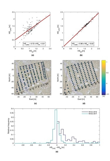
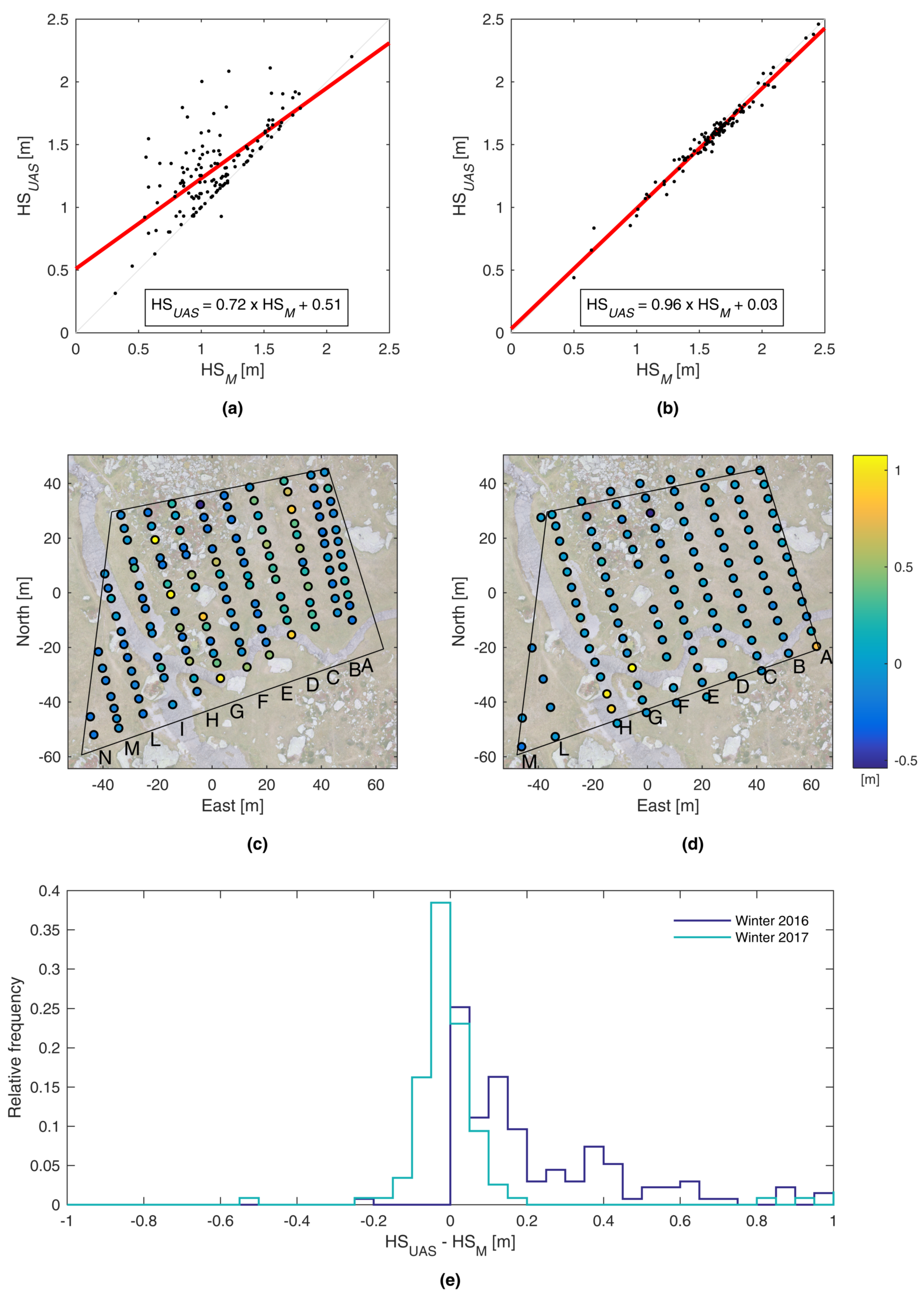
3.3. UAS vs. Manual Probing

Figure 5a shows the scatter plot between UAS-based (henceforth, HS U A S ) and manual (henceforth, HS M ) measurements of HS during the 2016 winter survey. A linear regression between these two datasets reads HS U A S = 0.72 × HS M + 0.51 (R 2 = 0.53). While these statistics show that the two datasets are correlated (73%), the difference between the data increases with a decreasing HS M . This plot also shows that UAS-based HS is generally greater than the manual one, i.e., HS U A S − HS M > 0 in ∼89% of the data. Figure 5b reports the same statistics using the 2017 snow survey: the linear regression between HS U A S and HS M reads HS U A S = 0.93 × HS M + 0.069 (R 2 = 0.97). In this case, the two datasets shows a much higher correlation (98%).
The mean difference between the UAS-based DSM and the 135 manual measurements (henceforth, HS U A S − HS M ) in 2016 reads 0.20 m, whereas the standard deviation is equal to 0.24 m. This translates into a RMSE equal to 0.31 m. About 39% of the measurements are between zero and 0.12 m (the median), with maximum and minimum differences equal to ∼1 m and −0.23 m, respectively (Figure 5e).
Figure 5c shows the spatial distribution of the differences between the UAS-based DSM and manual measurements for this first snow survey. Along courses A, B, E, F, I, L, M and N (Group 1), differences are smaller and more spatially homogeneous than along courses C, D, G, and H (Group 2, see Table 4). Because the measurement protocol as well as the manual probe were the same for all the courses, this discrepancy cannot be easily explained by a measurement error. While the differences are clustered along these courses, no evident spatial pattern in vegetation or soil coverage emerges that could clearly explain this mismatch.
The 2016 snow season at the study site was marked by an early snowpack (October 2015) that persisted at the site up to January 2016 and created a shallow, dense base layer (up to ∼10–15 cm thick). Between January and April 2016, the snowpack increased up to ∼150 cm, but both melt-freeze and rain-on-snow events occurred over the study area, especially in early April. Both processes, together with water retention at layer transitions due to capillary barriers [63], favor the development of ice layers [64]. While no pit was excavated during this first field survey due to time constraints, ice layers were observed close to the two streams crossing the study area, where the snow cover was patchy. The random occurrence of ice layers, coupled with slope redistribution of water in snow [65], may have impeded the full penetration of manual probes into snow, hence a systematic underestimation of snow depth [66].
During the second field survey in 2017, the mean difference between HS U A S and HS M was equal to 0.01 m, with a standard deviation equal to 0.20 m. This translates into a RMSE equal to 0.20 m (see Table 5). The maximum difference is equal to 0.52 m, while the minimum is equal to −1.08 m. During this second survey, the locations of maximum and minimum differences were more clearly correlated with topography, corresponding either to bushes or to the stream bed, which are both conditions that are prone to noise in manual probing as well as in DSMs. Both bushes and streams present complex elevation differences between winter and summer DSMs that may not be entirely due to snowpack, including potential micro-topographic variations in the surface of stream beds due to seasonal transport of sediments or larger rocks. This complicates the comparison at these specific locations as probing is expected to reach the ground surface, while HS U A S is the result of a differentiation between DSMs (e.g., photogrammetry reconstructs the surface of bushes, whereas probes are supposed to reach the underlying ground surface). If these outliers are removed from the sample, RMSE, minimum difference, and maximum difference decrease to 0.06 m, −0.72 m, and 0.19 m, respectively. One pit was excavated close to the study area during this second snow survey and no ice layer was found at any depth.

4. Discussion

Our results show that both UAS photogrammetric flights and a new, state-of-the-art scanning device capable of millimetric accuracy (MultiStation, [60]) can measure snowpack distribution at cm scale with mutually consistent results (maximum RMSE of 0.036 between point clouds). The comparison between UAS flights and manual sampling show higher RMSEs, in agreement with what reported before by e.g., [49] (0.14 m), [50] (less than 0.15 on rocks and less than 0.3 m on grass), [52] (0.22 m in open areas and 0.42 m in forests), or [51] (between 0.085 m and 0.137 m) [53] reported a median difference of −0.11 m and a standard deviation of 0.62 m, whereas [55] found accuracies between 0.10 m and 0.25 m on three Swiss glaciers—including both snow and bare ice.
This finding expands existing comparisons between UAS flights and other techniques on snow, which have focused on either manual sampling (see previous paragraph) or terrestrial laser scanners, capable of centrimetric accuracy [28,54]. A MS was used here on snow for the first time, to our knowledge. Such a high precision suggests that SfM techniques can now correctly solve the potentially more complex matching of images on a homogeneous surface, such as snow. This statement is supported by the standard deviations of the residuals between the UAS and the MS point clouds, which are comparable for both the summer and all winter cases.
The obtained RMSE between UAS flights and the MS is significantly smaller than those reported by [54], who compared four UAS flights at different wavelengths and shadow conditions with a TLS (RMSE between 0.18 m and 0.77 m). [28] expanded on this comparison involving 12 flights with visible and near-infrared cameras (accuracy below 0.29 m in full sunlight). On the one hand, our results show the expected increased accuracy of a MultiStation compared to a TLS and further support the high agreement between scanning and photogrammetric techniques on snow. On the other hand, results were obtained under optimal illumination conditions, whereas [28] show that the accuracy of UAS flights decreases under suboptimal illumination (accuracy of 0.49 and 0.37 m for DSMs and snow-depth maps at visible wavelength). Comparing UAS flights with a MultiStation under such conditions is an important direction of future work. It is worth noting that the error distribution over the reconstructed surface is homogeneous in case of a flight planned and realized considering appropriate overlapping and a constant flight height (as for the case here presented). On the contrary, the precision of a MS or a TLS depends on the distance between the station point and the investigated object (i.e., the distance traveled by the laser beam), on the incidence angle and on the material reflective properties.
Compared with most previous comparisons between UAS flights and manual probing, we focused here on a relatively dense grid. For example, [48] used 37 measurements over 6900 m 2 (0.5 pt/100 m 2 ), [23] took between 0.04 pt/100 m 2 and 0.11 pt/100 m 2 , and [52] took between 0.04 pt/100 m 2 and 0.2 pt/100 m 2 . [51] considered wide areas (0.65 km 2 and 0.32 km 2 ), but one of the two study sites included intensive plots, which is comparable to our survey. [28] also considered an intensive study plot with an average spacing of 18 m over 0.12 km 2 . Because the spatial variability of snow may be very large even over short distances [8], the outcome of a comparison between UAS and manual probing may change with the spatial resolution of manual data. However, these surveys revealed that increasing the number of points does not significantly affect the overall precision of the survey (i.e., the RMSE). UAS represents a competitive choice among existing techniques for high-precision remote sensing of snow at high resolution.
These surveys focused on snow depth, one of the two key variables that are routinely monitored by operational services all around the world—the second being Snow Water Equivalent. In California, for example, the California Snow Cooperative Survey performs snow-depth and SWE manual courses at monthly time scale over the entire Sierra Nevada and southern Cascade (http://cdec.water.ca.gov/snow/). Over the same mountain range, the Airborne Snow Observatory measures snow depth every two weeks during the snowmelt season on selected catchments using LiDAR scans [62]. Over European Alps, various agencies routinely manually measure snow depth for avalanche and hydrologic forecasting (http://www.avalanches.org/eaws/en/main.php). While SWE is the primary variable of interest for hydrologic applications, snow depth is a key variable for avalanche forecasting [20]. Because snow density is generally less variable in space than snow depth [67,68], knowledge of snow depth distribution can also potentially be converted to SWE via empirical regressions [69] or dynamic models [62]. In this context, portable, low-cost techniques, such as UAS and a MS, can fill an important gap between laborious, manual measurements and large-scale surveys at lower resolution using satellites or manned aircrafts. Yet, snow-density estimates using models currently represent the most important source of uncertainty when converting LiDAR-based snow depth to SWE [70]: coupling these devices with co-located measurements of density is therefore an important direction of future development.

5. Conclusions

We compared UAS-based photogrammetry and a MultiStation (MS) in measuring snow-depth distribution over a sample plot (6700 m 2 ). Two different surveys at peak accumulation were performed in spring 2016 and 2017, whereas a survey in summer 2016 with both instruments defined the reference, bare ground. We collected a relatively dense network of manual measurements of snow depth (135 pt in 2016 and 115 pt in 2017) to compare both techniques with the standard, traditional probing method. While several comparisons between UAS photogrammetry and manual probing are available in the literature, a MS was tested on snow for the first time.
UAS-based photogrammetry and the MS show highly consistent results: the mean of the residuals between the MS and UAS point clouds is not significantly different from zero for the summer survey (0.004 m vs. a standard deviation of 0.020 m). For the winter cases, a bias equal to 0.026 m was found in 2016, which is mainly due to ongoing snowmelt (time difference of three hours). The mean of the residuals for the 2017 snow survey is much smaller, i.e., −0.003 m when comparing clouds. The standard deviations of the residuals are of the order of the GSD for all the cases. These small variations are related to different soil coverage and illumination conditions, which cause different tie-point matching quality. The Root Mean Square Error (RMSE) between UAS and MS point clouds on snow are less or equal than 0.036 m. When comparing the photogrammetric DSMs with the MS point clouds, an increase in the mean and the standard deviations of the residuals was found. This is because a DSM interpolates a point cloud and introduces a smoothing effect, especially in correspondence of abrupt terrain variations.
The comparison between the UAS map and manual measurements shows RMSEs of the order of 0.30–0.20 m, which agrees with previous works. The mean difference between the two datasets is equal to 0.20 m and 0.01 m in 2016 and 2017, respectively. Larger differences between UAS and manual data of snow depth could be explained by canopy, topographic features, such as rocks, ice layers, and proximity to the river bed. When excluding areas of potential outliers, the observed RMSE decreases to 0.17 m in 2016 and 0.06 m in 2017. These results support the use of UAS and MS laser scanning as a support to traditional manual surveys for high-precision high-resolution monitoring of snow depth.

Author Contributions

C.D.M. conceived the study. A.B., A.C., C.D.M., P.M., L.P., and M.P. designed the field surveys. F.A., A.B., A.C., C.D.M., P.M., D.P., D.P., L.P., and L.R. performed the field surveys (realization of the geodetic networks, MulitStation acquisitions and snow height measurements). D.P. realized the photogrammetric flights. D.P. performed the photogrammetric processing. L.R. computed the geodetic network adjustment. F.A., C.D.M., D.P., L.P. and L.R. contributed to overall data analysis. The manuscript has been prepared with the contribution of all co-authors.

Acknowledgments

The authors would like to thank the students who participated to the Summer School “Design and realization of topographic surveys” (ed. 2015 and 2016) and to the 11th and 12th cycles of Alta Scuola Politecnica. We also thank Arpa Piemonte for sharing the daily weather data (season 2015–2016) and the observed profile of snow properties on 24th March 2016 at Rifugio Zamboni. Fruitful discussions and field logistical support by Mauro Spanò is acknowledged. We also would like to acknowledge discussions with the Harmosnow Consortium, COST ES 1404 action (www.harmosnow.eu) “A European network for a harmonised monitoring of snow for the benefit of climate change scenarios, hydrology and numerical weather prediction”. The project was supported by educational funds from Alta Scuola Politecnica (11th and 12th cycles—project DREAM and DREAM2).

Conflicts of Interest

The authors declare no conflict of interest.

References

  1. DeWalle, D.R.; Rango, A. Principles of Snow Hydrology; Cambridge University Press: Cambridge, UK, 2011. [Google Scholar]
  2. Fierz, C.; Armstrong, R.; Durand, Y.; Etchevers, P.; Greene, E.; McClung, D.; Nishimura, K.; Satyawali, P.; Sokratov, S. The International Classification for Seasonal Snow on the Ground; Technical Report, IHP-VII Technical Documents in Hydrology N 83, IACS Contribution N 1; UNESCO/IHP: Paris, France, 2009. [Google Scholar]
  3. Avanzi, F.; De Michele, C.; Ghezzi, A.; Jommi, C.; Pepe, M. A processing-modeling routine to use SNOTEL hourly data in snowpack dynamic models. Adv. Water Resour. 2014, 73, 16–29. [Google Scholar] [CrossRef]
  4. Morin, S.; Lejeune, Y.; Lesaffre, B.; Panel, J.M.; Poncet, D.; David, P.; Sudul, M. An 18-yr long (1993–2011) snow and meteorological dataset from a mid-altitude mountain site (Col de Porte, France, 1325 m alt.) for driving and evaluating snowpack models. Earth Syst. Sci. Data 2012, 4, 13–21. [Google Scholar] [CrossRef]
  5. Johnson, J.B.; Marks, D. The detection and correction of snow water equivalent pressure sensor errors. Hydrol. Process. 2004, 18, 3513–3525. [Google Scholar] [CrossRef]
  6. López Moreno, J.I.; Fassnacht, S.R.; Beguería, S.; Latron, J.B.P. Variability of snow depth at the plot scale: Implications for mean depth estimation and sampling strategies. Cryosphere 2011, 5, 617–629. [Google Scholar] [CrossRef] [Green Version]
  7. Grünewald, T.; Lehning, M. Are flat-field snow depth measurements representative? A comparison of selected index sites with areal snow depth measurements at the small catchment scale. Hydrol. Process. 2015, 29, 1717–1728. [Google Scholar] [CrossRef]
  8. López Moreno, J.I.; Revuelto, J.; Fassnacht, S.R.; Azorín-Molina, C.; Vicente-Serrano, S.M.; Morán-Tejeda, E.; Sexstone, G.A. Snowpack variability across various spatio-temporal resolutions. Hydrol. Process. 2015, 29, 1213–1224. [Google Scholar] [CrossRef]
  9. Helbig, N.; van Herwijnen, A. Subgrid parameterization for snow depth over mountainous terrain from flat field snow depth. Water Resour. Res. 2017. [Google Scholar] [CrossRef]
  10. Malek, S.A.; Avanzi, F.; Brun-Laguna, K.; Maurer, T.; Oroza, C.A.; Hartsough, P.C.; Watteyne, T.; Glaser, S.D. Real-time Alpine measurement system using wireless sensor networks. Sensors 2017, 17, 2583. [Google Scholar] [CrossRef] [PubMed]
  11. Kattelmann, R. Spatial variability of snow-pack outflow at a site in Sierra Nevada, USA. Ann. Glaciol. 1989, 13, 124–128. [Google Scholar] [CrossRef]
  12. Schweizer, J.; Kronholm, K.; Bruce Jamieson, J.; Birkeland, K.W. Review of spatial variability of snowpack properties and its importance for avalanche formation. Cold Reg. Sci. Technol. 2008, 51, 253–272. [Google Scholar] [CrossRef]
  13. Grünewald, T.; Schirmer, M.; Mott, R.; Lehning, M. Spatial and temporal variability of snow depth and ablation rates in a small mountain catchment. Cryosphere 2010, 4, 215–225. [Google Scholar] [CrossRef]
  14. Scipión, D.; Mott, R.; Lehning, M.; Schneebeli, M.; Berne, A. Seasonal small-scale spatial variability in alpine snowfall and snow accumulation. Water Resour. Res. 2013, 49, 1446–1457. [Google Scholar] [CrossRef]
  15. Bavera, D.; De Michele, C. Snow water equivalent estimation in the Mallero basin using snow gauge data and MODIS images and fieldwork validation. Hydrol. Process. 2009, 23, 1961–1972. [Google Scholar] [CrossRef]
  16. Dietz, A.J.; Kuenzer, C.; Gessner, U.; Dech, S. Remote sensing of snow—A review of available methods. Int. J. Remote Sens. 2012, 33, 4094–4134. [Google Scholar] [CrossRef]
  17. Sturm, M. White water: Fifty years of snow research in WRR and the outlook for the future. Water Resour. Res. 2015, 51, 4948–4965. [Google Scholar] [CrossRef]
  18. Jörg, P.; Fromm, R.; Sailer, R.; Schaffhauser, A. Measuring snow depth with a terrestrial laser ranging system. In Proceedings of the International Snow Science Workshop, Telluride, CO, USA, 1–6 October 2006; pp. 452–460. [Google Scholar]
  19. Jaakkola, A.; Hyyppä, J.; Puttonen, E. Measurement of snow depth using a low-cost mobile laser scanner. IEEE Geosci. Remote Sens. Lett. 2014, 11, 587–591. [Google Scholar] [CrossRef]
  20. Prokop, A.; Schirmer, M.; Rub, M.; Lehning, M.; Stocker, M. A comparison of measurement methods: Terrestrial laser scanning, tachymetry and snow probing for the determination of the spatial snow-depth distribution on slopes. Ann. Glaciol. 2008, 49, 210–216. [Google Scholar] [CrossRef]
  21. Grünewald, T.; Stötter, J.; Pomeroy, J.W.; Dadic, R.; Baños, I.M.; Marturiá, J.; Spross, M.; Hopkinson, C.; Burlando, P.; Lehning, M. Statistical modelling of the snow depth distribution in open alpine terrain. Hydrol. Earth Syst. Sci. 2013, 17, 3005–3021. [Google Scholar] [CrossRef]
  22. Revuelto, J.; Vionnet, V.; López-Moreno, J.I.; Lafaysse, M.; Morin, S. Combining snowpack modeling and terrestrial laser scanner observations improves the simulation of small scale snow dynamics. J. Hydrol. 2016, 533, 291–307. [Google Scholar] [CrossRef]
  23. Bühler, Y.; Marty, M.; Egli, L.; Veitinger, J.; Jonas, T.; Thee, P.; Ginzler, C. Snow depth mapping in high-alpine catchments using digital photogrammetry. Cryosphere 2015, 9, 229–243. [Google Scholar] [CrossRef]
  24. Nolan, M.; Larsen, C.; Sturm, M. Mapping snow depth from manned aircraft on landscape scales at centimeter resolution using structure-from-motion photogrammetry. Cryosphere 2015, 9, 1445–1463. [Google Scholar] [CrossRef]
  25. Machguth, H.; Eisen, O.; Paul, F.; Hoezle, M. Strong spatial variability of snow accumulation observed with helicopter-borne GPR on two adjacent Alpine glaciers. Geophys. Res. Lett. 2006, 33, L13503. [Google Scholar] [CrossRef]
  26. Farinotti, D.; Magnusson, J.; Huss, M.; Bauder, A. Snow accumulation distribution inferred from time-lapse photography and simple modelling. Hydrol. Process. 2010, 24, 2087–2097. [Google Scholar] [CrossRef]
  27. Parajka, J.; Haas, P.; Kirnbauer, R.; Jansa, J.; Blöschl, G. Potential of time-lapse photography of snow for hydrological purposes at the small catchment scale. Hydrol. Process. 2012, 26, 3327–3337. [Google Scholar] [CrossRef]
  28. Adams, M.S.; Bühler, Y.; Fromm, R. Multitemporal accuracy and precision assessment of unmanned aerial system photogrammetry for slope-scale snow depth maps in Alpine terrain. Pure Appl. Geophys. 2017. [Google Scholar] [CrossRef]
  29. Thamm, H.; Judex, M. The “low cost drone”—An interesting tool for process monitoring in a high spatial and temporal resolution. In Proceedings of the ISPRS Commission VII Mid-Term Symposium “Remote Sensing from Pixels to Processes”, Enschede, The Netherlands, 8–11 May 2006; pp. 140–144. [Google Scholar]
  30. Newcombe, L. Green fingered UAVs. In Unmanned Vehicle; 2007. [Google Scholar]
  31. Grenzdörffer, G.; Engel, A.; Teichert, B. The photogrammetric potential of low-cost UAVs in forestry and agriculture. Int. Arch. Photogramm. Remote Sens. Spat. Inf. Sci. 2008, 31, 1207–1214. [Google Scholar]
  32. Gini, R.; Passoni, D.; Pinto, L.; Sona, G. Use of unmanned aerial systems for multispectral survey and tree classification: A test in a park area of northern Italy. Eur. J. Remote Sens. 2014, 47, 251–269. [Google Scholar] [CrossRef]
  33. Niethammer, U.; Rothmund, S.; James, M.; Travelletti, J.; Joswig, M. UAV-based remote sensing of landslides. Int. Arch. Photogramm. Remote Sens. Spat. Inf. Sci. 2010, 38, 496–501. [Google Scholar]
  34. Molina, P.; Colomina, I.; Victoria, T.; Skaloud, J.; Kornus, W.; Prades, R.; Aguilera, C. Searching lost people with UAVS: The system and results of the CLOSE-SEARCH project. Int. Arch. Photogramm. Remote Sens. Spat. Inf. Sci. 2012, 39, 441–446. [Google Scholar] [CrossRef]
  35. Nex, F.; Remondino, F. UAV for 3D mapping applications: A review. Appl. Geomat. 2014, 6, 1–15. [Google Scholar] [CrossRef]
  36. Pagliari, D.; Rossi, L.; Passoni, D.; Pinto, L.; De Michele, C.; Avanzi, F. Measuring the volume of flushed sediments in a reservoir using multi-temporal images acquired with UAS. Geomat. Nat. Hazards Risk 2017, 8, 150–166. [Google Scholar] [CrossRef]
  37. Berni, J.A.; Zarco-Tejada, P.J.; Suárez, L.; Fereres, E. Thermal and narrowband multispectral remote sensing for vegetation monitoring from an unmanned aerial vehicle. IEEE Trans. Geosci. Remote Sens. 2009, 47, 722–738. [Google Scholar] [CrossRef] [Green Version]
  38. Tauro, F.; Porfiri, M.; Grimaldi, S. Surface flow measurements from drones. J. Hydrol. 2016, 540, 240–245. [Google Scholar] [CrossRef]
  39. Eisenbeiß, H. UAV Photogrammetry. Ph.D. Thesis, ETH Zurich, Zurich, Switzerland, 2009. [Google Scholar]
  40. Colomina, I.; Molina, P. Unmanned aerial systems for photogrammetry and remote sensing: A review. ISPRS J. Photogramm. Remote Sens. 2014, 92, 79–97. [Google Scholar] [CrossRef]
  41. Tao, T.S.; Hansman, R.J. Development of an In-Flight-Deployable Micro-UAV. In Proceedings of the 54th AIAA Aerospace Sciences Meeting, San Diego, CA, USA, 4–8 January 2016; p. 1742. [Google Scholar]
  42. Lowe, D.G. Distinctive image features from scale-invariant keypoints. Int. J. Comput. Vis. 2004, 60, 91–110. [Google Scholar] [CrossRef]
  43. Bay, H.; Ess, A.; Tuytelaars, T.; Van Gool, L. Speeded-up robust features (SURF). Comput. Vis. Image Underst. 2008, 110, 346–359. [Google Scholar] [CrossRef]
  44. Hartley, R.; Zisserman, A. Multiple View Geometry in Computer Vision; Cambridge University Press: Cambridge, UK, 2003. [Google Scholar]
  45. Koenderink, J.J.; Van Doorn, A.J. Affine structure from motion. JOSA A 1991, 8, 377–385. [Google Scholar] [CrossRef]
  46. El-Gayar, M.; Soliman, H.; Meky, N. A comparative study of image low level feature extraction algorithms. Egypt. Inform. J. 2013, 14, 175–181. [Google Scholar] [CrossRef]
  47. Lingua, A.M.; Marenchino, D.; Nex, F.C. A Comparison between “old and new” feature extraction and matching techniques in photogrammetry. RevCAD J. Geod. Cadastre 2009, 9, 43–52. [Google Scholar]
  48. Vander Jagt, B.; Lucieer, A.; Wallace, L.; Turner, D.; Durand, M. Snow depth retrieval with UAS using photogrammetric techniques. Geosciences 2015, 5, 264–285. [Google Scholar] [CrossRef]
  49. De Michele, C.; Avanzi, F.; Passoni, D.; Barzaghi, R.; Pinto, L.; Dosso, P.; Ghezzi, A.; Gianatti, R.; Della Vedova, G. Using a fixed-wing UAS to map snow depth distribution: An evaluation at peak accumulation. Cryosphere 2016, 10, 511–522. [Google Scholar] [CrossRef]
  50. Bühler, Y.; Adams, M.S.; Bösch, R.; Stoffel, A. Mapping snow depth in alpine terrain with unmanned aerial systems (UASs): Potential and limitations. Cryosphere 2016, 10, 1075–1088. [Google Scholar] [CrossRef]
  51. Harder, P.; Schirmer, M.; Pomeroy, J.; Helgason, W. Accuracy of snow depth estimation in mountain and prairie environments by an unmanned aerial vehicle. Cryosphere 2016, 10, 2559–2571. [Google Scholar] [CrossRef]
  52. Lendzioch, T.; Langhammer, J.; Jenicek, M. Tracking forest and open area effects on snow accumulation by unmanned aerial vehicle photogrammetry. Int. Arch. Photogramm. Remote Sens. Spat. Inf. Sci. 2016, 41, 917. [Google Scholar] [CrossRef]
  53. Marti, R.; Gascoin, S.; Berthier, E.; de Pinel, M.; Houet, T.; Laffly, D. Mapping snow depth in open alpine terrain from stereo satellite imagery. Cryosphere 2016, 10, 1361–1380. [Google Scholar] [CrossRef] [Green Version]
  54. Bühler, Y.; Adams, M.S.; Stoffel, A.; Boesch, R. Photogrammetric reconstruction of homogenous snow surfaces in alpine terrain applying near-infrared UAS imagery. Int. J. Remote Sens. 2017, 38, 3135–3158. [Google Scholar] [CrossRef]
  55. Gindraux, S.; Boesch, R.; Farinotti, D. Accuracy assessment of digital surface models from unmanned aerial vehicles’ imagery on glaciers. Remote Sens. 2017, 9, 186. [Google Scholar] [CrossRef]
  56. Smith, F.; Cooper, C.; Chapman, E. Measuring Snow Depths by Aerial Photography. In Proceedings of the 35th Annual Meeting, Western Snow Conference, Boise, ID, USA, 18–20 April 1967; pp. 66–72. [Google Scholar]
  57. Cline, D. Measuring alpine snow depths by digital photogrammetry. Part 1: Conjugate point identification. In Proceedings of the Eastern Snow Conference, Quebec City, QC, Canada, 8–10 June 1993; pp. 265–271. [Google Scholar]
  58. Cline, D.W. Digital photogrammetric determination of Alpine snowpack distribution for hydrologic modeling. In Proceedings of the Western Snow Conference, Colorado State University, Fort Collins, CO, USA, 18–21 April 1994. [Google Scholar]
  59. Grimm, D.E. Leica Nova MS50: The world’s first MultiStation. GeoInformatics 2013, 16, 22. [Google Scholar]
  60. Fagandini, R.; Federici, B.; Ferrando, I.; Gagliolo, S.; Pagliari, D.; Passoni, D.; Pinto, L.; Rossi, L.; Sguerso, D. Evaluation of the Laser Response of Leica Nova MultiStation MS60 for 3D Modelling and Structural Monitoring. In International Conference on Computational Science and Its Applications; Springer: Berlin, Germany, 2017; pp. 93–104. [Google Scholar]
  61. Federman, A.; Quintero, M.S.; Kretz, S.; Gregg, J.; Lengies, M.; Ouimet, C.; Laliberte, J. UAV photgrammetric workflows: A best practice guideline. Int. Arch. Photogramm. Remote Sens. Spat. Inf. Sci. 2017, 42. [Google Scholar] [CrossRef]
  62. Painter, T.H.; Berisford, D.F.; Boardman, J.W.; Bormann, K.J.; Deems, J.S.; Gehrke, F.; Hedrick, A.; Joyce, M.; Laidlaw, R.; Marks, D.; et al. The airborne snow observatory: Fusion of scanning lidar, imaging spectrometer, and physically-based modeling for mapping snow water equivalent and snow albedo. Remote Sens. Environ. 2016, 184, 139–152. [Google Scholar] [CrossRef]
  63. Avanzi, F.; Hirashima, H.; Yamaguchi, S.; Katsushima, T.; De Michele, C. Observations of capillary barriers and preferential flow in layered snow during cold laboratory experiments. Cryosphere 2016, 10, 2013–2026. [Google Scholar] [CrossRef]
  64. Wever, N.; Würzer, S.; Fierz, C.; Lehning, M. Simulating ice layer formation under the presence of preferential flow in layered snowpacks. Cryosphere 2016, 10, 2731–2744. [Google Scholar] [CrossRef]
  65. Eiriksson, D.; Whitson, M.; Luce, C.H.; Marshall, H.P.; Bradford, J.; Benner, S.G.; Black, T.; Hetrick, H.; McNamara, P. An evaluation of the hydrologic relevance of lateral flow in snow at hillslope and catchment scales. Hydrol. Process. 2013, 27, 640–654. [Google Scholar] [CrossRef]
  66. National Oceanic and Atmospheric Administration. Snow Measurement Guidelines for National Weather Service Surface Observing Programs; National Oceanic and Atmospheric Administration: Silver Spring, MD, USA, 2013. [Google Scholar]
  67. Mizukami, N.; Perica, S. Spatiotemporal characteristics of snowpack density in the mountainous regions of the Western United States. J. Hydrometeorol. 2008, 9, 1416–1426. [Google Scholar] [CrossRef]
  68. De Michele, C.; Avanzi, F.; Ghezzi, A.; Jommi, C. Investigating the dynamics of bulk snow density in dry and wet conditions using a one-dimensional model. Cryosphere 2013, 7, 433–444. [Google Scholar] [CrossRef]
  69. Sturm, M.; Taras, B.; Liston, G.E.; Derksen, C.; Jonas, T.; Lea, J. Estimating snow water equivalent using snow depth data and climate classes. J. Hydrometeorol. 2010, 11, 1380–1394. [Google Scholar] [CrossRef]
  70. Raleigh, M.S.; Small, E.E. Snowpack density modeling is the primary source of uncertainty when mapping basin-wide SWE with lidar. Geophys. Res. Lett. 2017, 44, 3700–3709. [Google Scholar] [CrossRef]
Figure 1. Topography of the surveyed area during summer 2016 ((a), top-left), winter 2016 ((b), top-right) and winter 2017 ((c), bottom-right). The boundaries of the study area are in black. Red dots denote the station points of the MultiStation, whereas the blue triangle represents the point used as angular reference. No bare-soil survey was performed during summer 2017.
Remotesensing 10 00765 g001
Figure 2. Digital Surface Models from the UAS surveys during summer 2016 ((a), top-left), winter 2016 ((b), top-right) and winter 2017 ((c), bottom-right). The color map represents surface height (ASL). Contour lines (grey) are reported with an equidistant interval of 2 m. No bare-soil survey was performed during summer 2017.
Remotesensing 10 00765 g002
Figure 3. Height differences between the MultiStation (MS) dataset and the photogrammetric products for all surveys. C1 compares the MultiStation and the photogrammetric point clouds, whereas C2 compares the MultiStation point cloud with the DSM from UAS data.
Remotesensing 10 00765 g003
Figure 4. Histograms of the residuals between the MultiStation scan and the DSM from UAS data (C2) for each of the three surveys (a). Scatter plot of UAS-based vs. MS-based heights (ASL) for both winter and summer cases (b).
Remotesensing 10 00765 g004
Figure 5. Evaluation of UAS data using manual probing. (a,b): Scatter plots between UAS-based and manual measurements of HS for 2016 and 2017, respectively (regression line in red). (c,d): Spatial distribution of the differences between UAS-based and manual measurements of snow depth. The color legend represents the differences between UAS and manual probing. (e): Histograms of the differences between UAS-based and manual measurements of snow depth for both surveys.
Remotesensing 10 00765 g005
Table 1. Schedule of the two field surveys on snow (all times are local).
TaskWinter 2016Winter 2017
UAS flights12 PM12 PM
MS surveys12 PM to 1 PM12 PM to 1 PM
Manual probing1 PM to 4 PM1 PM to 4 PM
Table 2. Root Mean Square Error between the measured and estimated coordinates of Ground Control Points (GCPs).
Flight SeasonEast (m)North (m)Height (m)
Summer 20160.0100.0070.005
Winter 20160.0170.0100.004
Winter 20170.0060.0070.009
Table 3. Statistics of the winter and summer comparisons between the photogrammetric products and data from the MultiStation.
Point Cloud (C1)DSM (C2)
SurveyMean (m)St. Dev. (m)RMSE (m)Mean (m)St. Dev. (m)RMSE (m)
Summer 20160.0040.0200.0200.0010.0680.068
Winter 20160.0260.0250.0360.0410.0560.069
Winter 2017−0.0030.0150.015−0.0050.0250.025
Table 4. Statistics of the differences between UAS and manual measurements in 2016. Results are separated between areas with significantly smaller errors (Group 1, courses A, B, E, F, I, L, M and N—84 samples) and areas with larger errors (Group 2, courses C, D, G, and H—51 samples).
GroupMean (m)St. Dev. (m)RMSE (m)
10.110.140.17
20.360.270.45
Table 5. Statistics of the differences between UAS and manual measurements in 2017. Results are reported with or without outliers (8 samples out of 115).
Mean (m)St. Dev. (m)RMSE (m)
With outliers0.010.200.20
Without outliers0.040.050.06

