Hyperspectral Images Classification Based on Dense Convolutional Networks with Spectral-Wise Attention Mechanism

Abstract

Hyperspectral images (HSIs) data that is typically presented in 3-D format offers an opportunity for 3-D networks to extract spectral and spatial features simultaneously. In this paper, we propose a novel end-to-end 3-D dense convolutional network with spectral-wise attention mechanism (MSDN-SA) for HSI classification. The proposed MSDN-SA exploits 3-D dilated convolutions to simultaneously capture the spectral and spatial features at different scales, and densely connects all 3-D feature maps with each other. In addition, a spectral-wise attention mechanism is introduced to enhance the distinguishability of spectral features, which improves the classification performance of the trained models. Experimental results on three HSI datasets demonstrate that our MSDN-SA achieves competitive performance for HSI classification.

1. Introduction

Hyperspectral images (HSIs) have hundreds of continuous observation bands throughout the electromagnetic spectrum with high spectral resolution [1]. Based on such abundant spectral bands, HSIs have been widely used in various applications, including agriculture development [2], mineral resource exploitation [3], and environmental earth sciences [4]. Supervised land cover classification is one of the most significant topics in hyperspectral remote sensing. However, the redundancy of spectral band information combined with limited training samples [5,6] often poses a challenge to HSI classification.

Conventional HSI supervised classification models are often based on spectral information. Typical classifiers include those based on distance measure [7], k-nearest-neighbors [8], maximum likelihood criterion [9], and logistic regression [10]. To improve classification performance, Random Forests (RF) [11], and AdaBoost [12], which are ensemble learning or multiple classifier methods, have been found to be effective for HSI classification.

However, classification algorithms based on spectral information exploiting only the spectral information fail to capture the important spatial variability perceived for high-resolution data. Furthermore, as HSIs are typically presented in the format of 3-D cubes, it is reasonable to combine the abundant spectral features and spatial features in complementary form to improve the performance of HSI classification. For example, spectral-spatial combined features can be extracted from the HSI, at different frequencies and scales, by a series of 3-D discrete wavelet filters [13,14], 3-D Gabor filters [15,16], or 3-D scattering wavelet filers [17]. In this way, a large number of feature cubes can be created, which contain important information about local signal changes in spectrum, space, and joint spectral-spatial correlations. This information is essential for tackling challenging classification tasks.

In recent years, deep convolutional neural networks with hierarchical feature learning capability have become the mainstream machine learning methods in the field of computer vision, and have achieved gratifying results in different tasks [18,19]. Compared with traditional manually engineered features, deep learning technology automatically learns hierarchical features from raw input data [20,21]. The great success of convolutional neural networks (CNNs) and their extensions have motivated remarkable efforts in spectral-spatial HSI classification [22]. For instance, Yang et al. [23] proposed a two-channel CNN framework, which extracts jointly the spectral features and spatial features from HSI. Chen et al. [24] and Li et al. [25] have utilized a 3-D convolutional kernel to learn the discriminative spectral-spatial features and classifications are performed in an end-to-end structure. Note that the method in [25] used relatively smaller spatial sized cubes as input and has fewer parameters to tune. Gao et al. [26] proposed a CNN based architecture, which benefits from the multiple inputs corresponding to various image features, and exploited the both spectral and spatial contextual information concurrently for HSI classification. Yang et al. [27] advocated a recurrent 3-D CNN (R-3-D-CNN) model, which can often outperform other models and converge faster because of its 3-D convolutional operators and the recurrent network structure. However, it is reported that R-3-D-CNN requires more training samples than the traditional machine learning methods [27].

Although deep learning models have finally shown promising performance in HSI classification, they have an insatiable hunger for larger and larger data sets, while the available labeled samples are rather limited in the HSIs. Thus, the problem of small training samples restricts the deep learning based HSI classification approaches to obtain better performance. To deal with this problem, Ma et al. [28] proposed a spatially updated deep auto-encoder for spectral-spatial feature extraction, by adding a sample similarity regularization mechanism and combining it with the collaborative representation-based classification to deal with the problem of small training sets. In [23], when training samples are limited, transfer learning is used, where low-level and mid-level features are transferred from other scenes. Pan et al. [29] proposed an ensemble deep learning based method, multi-grained network (MugNet) for limited training samples. To take full advantage of abundant unlabeled samples, they adopted a semi-supervised manner in the process of generating convolution kernels. Again, to deal with the problem of limited training samples, the concept of generative adversarial networks (GAN) has been extended to be a conditional model with semi-supervised classification methods by He et al. [30]. The authors trained a generator and a discriminator on spatial-spectral features obtained from HSI. Then, they added a softmax layer to the discriminator network at the end and fine-tuning the network to perform classification. In addition, Zhong et al. [31] proposed a supervised spectral-spatial residual network (SSRN) with consecutive spectral and spatial residual blocks to extract spectral and spatial features from HSI. It is reported that SSRN is more effective in the case of small training samples, which is due to the fact that SSRN contains residual connections [19] between each of the other convolutional layers so that residual blocks are constructed. The success of residual connections has demonstrated that combining the features of the lower layers can capture finer features.

In this paper, we propose a method to distill the dense connectivity [32] of the network and construct a novel learning architecture with dense connectivity for automated classification from 3-D HSI. In addition, considering the redundancy of the spectral bands in HSI, a new spectral-wise attention mechanism is added to the proposed network. As a result, this paper contributes in four major respects:

• We introduce a network architecture specifically designed for the 3-D patches of HSI. The network uses dilated convolutions to capture features at various patch scales, thereby obtaining multiple scales within a single layer. Dense connectivity connects 3-D feature maps learned from different layers, increasing the diversity of inputs in subsequent layers.
• A new spectral-wise attention mechanism is aiming to selectively emphasize informative spectral features and suppress less useful spectral features. The spectral-wise attention mechanism that applies soft weights on features is well suited and more efficient for the following HSI classification tasks. To the best of our knowledge, this is the first time an attention mechanism has been introduced for HSI classification.
• Experimental results on three HSI datasets demonstrate that our novel end-to-end 3-D dense convolutional network with spectral-wise attention mechanism (MSDN-SA) method outperforms the state-of-the-art methods.

The remainder of this paper is organized as follows. In Section 2, we briefly introduce the different connections and the spectral-attention mechanism in CNNs. In Section 3, we describe our MSDN-SA method in detail. In Section 4 and Section 5, we present and discuss the experimental results. Finally, in Section 6, the paper is summarized with an outline suggestion for future work.

2. Related Work

2.1. Residual Connections and Dense Connectivity in CNNs

Previous research [33,34,35] has shown that utilizing multi-level features in CNNs through skip-connections is effective for various vision tasks. Residual connections and dense connectivity act as two different connectivity patterns: both have been successfully used in challenging natural image processing tasks. Here, we briefly introduce these two connection concepts.

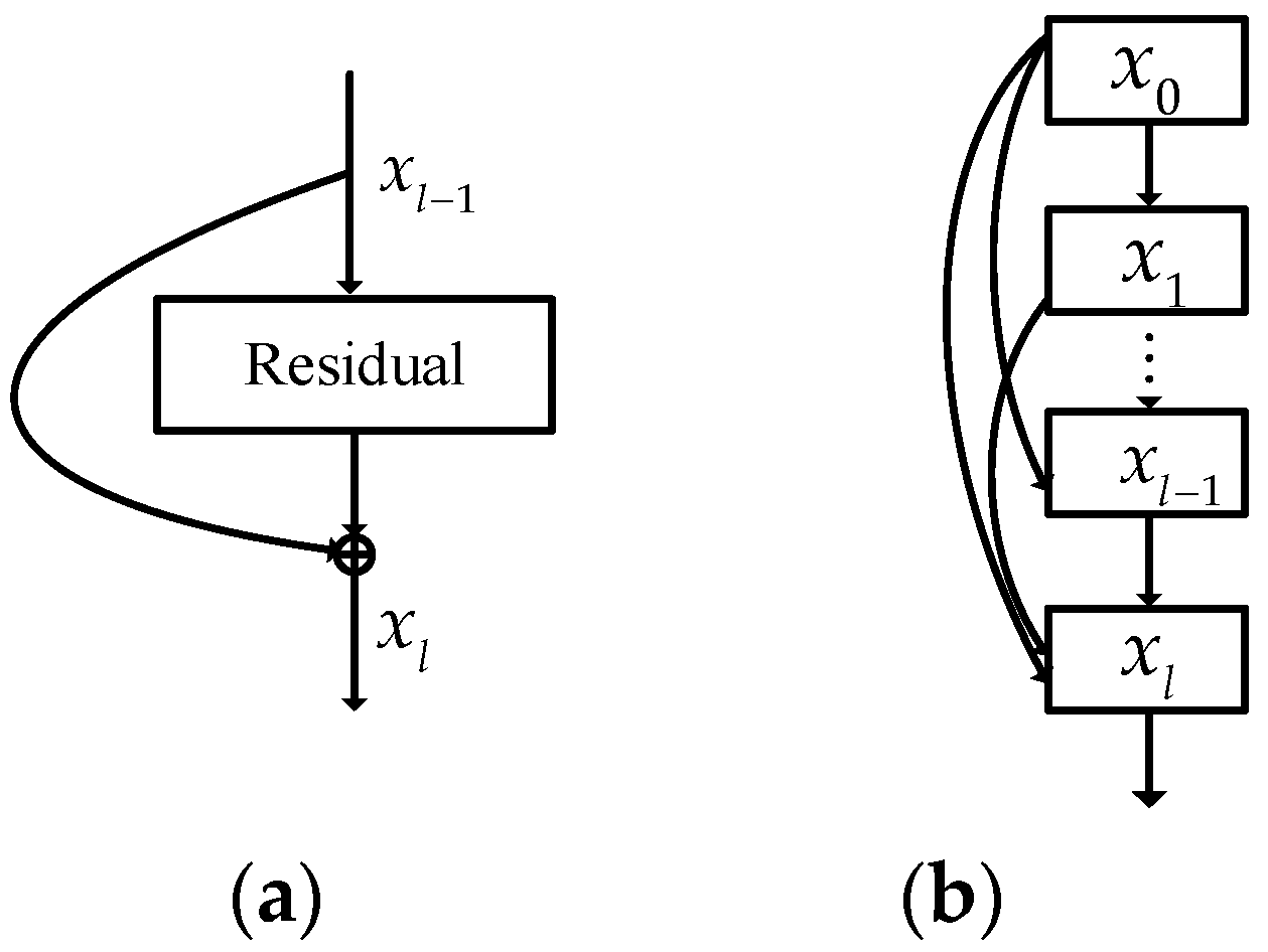
In principle, a residual connection (Figure 1a) adds a skip connection that bypasses the nonlinear transformations with an identity mapping. Reference layer inputs explicitly represent the layers as learning residual functions [19]. A residual connection can be formally expressed as:

$$x_l=h(x_{l-1})+F(x_{l-1}),$$

(1)

where $x_{l-1}$ and $x_l$ refer to the input and output of the l-th layer, respectively. The $h(x_{l-1})=x_{l-1}$ is an identity mapping function and the function $F(\cdot )$ represents a non-linear transformation which can be a composite function of operations such as Convolution (Conv), Batch Normalization (BN) [36], Rectified Linear Units (ReLU) [37], or Pooling [38]. By using residual connections, the gradient can flow directly from later to earlier layers through the identity function [19].

In order to maximize the flow of information between network layers, Gao et al. [32] proposed a series of dense connectivity from any layer to all subsequent layers (Figure 1b). Differing from the residual connections, which combine features through summation, dense connectivity combines features by concatenating them. Specifically, all previous feature maps of layers $x_0,\dots ,x_{l-1}$, can be used to compute the output of the l-th layer:

$$x_l=F(\{x_0,\dots ,x_{l-1}\}),$$

(2)

where $\{x_0,\dots ,x_{l-1}\}$ is the concatenation of all previous feature maps.

Each layer has direct access to the gradients from the loss function and the original input signal, leading to an implicit deep supervision. The work of [32] also allows features to be reused, while adding only a small set of feature maps to the network [32]. In addition, dense connectivity has a regularization parameter that reduces overfitting on tasks with small training data. Therefore, dense connectivity can be beneficial to perform HSI classification, especially with small training data.

2.2. Attention Mechanism

Evidence from human perception process [39] demonstrates the importance of an attention mechanism, which usually uses top-level information to guide a bottom-up feedforward process. An attention mechanism can be viewed as a tool to bias the allocation of available processing resources towards the most informative components of an input signal.

Recently, researchers have applied attention mechanism in deep neural networks. Generally, there are two categories of such work: spatial-based attention and channel-wise attention. Spatial-based attention mostly focuses on specific location scenes. Such mechanisms were the focus of early systems for image categorization [40], and were later shown to yield significant improvements for Visual Question Answering (VQA) and captioning [41,42,43]. Channel-wise attention is a complementary form of attention, which involves learning a task-specific modulation that is selectively applied to individual feature maps across the entire scene. Among them, Squeeze-and-Excitation (SE) network (recognized as ImageNet Large Scale Visual Recognition Competition (ILSVRC) winner), produces significant performance improvements for state-of-the-art deep architectures at slightly greater computational cost. SE block [44] is a novel architectural unit designed to improve the representational capacity of a network by enabling it to perform dynamic channel-wise feature recalibration.

On the basis of attention mechanism, many deep neural network structures have been proposed and widely used in various applications [43,44,45,46,47]. For example, Fu et al. [45] introduced a recurrent attention CNN, which can locate the discriminative region recurrently for fine-grained image recognition performance. Li et al. [46] introduced a global attention upsample module to guide the integration of low- and high-level features in semantic segmentation. Wang et al. [47] proposed a residual attention network, which is built by trunk-and-mask [48] attention mechanism to generate attention-aware features for Image Classification. It is worth mentioning that SE network is a lightweight gating mechanism [44], specialized to model channel-wise relationships in a computationally efficient manner and designed to enhance the representational power of modules throughout the network.

In the case of HSI, hundreds of spectral bands are directly used as input data for convolution, which inevitably carries some noise bands. Therefore, we are more concerned with the correlation of the spectral-wise features from HSI which are based on the 3-D feature maps. Inspired by the SE network, we propose a spectral-wise attention mechanism which will be discussed in detail in the next section.

3. Proposed Methods

In this section, we describe a novel 3-D network for HSI classification. There are two key components in our proposed method: dense convolutional network with dilated convolution and spectral-wise attention mechanism. The first part is dilated convolution [49] based on 3-D patches of an HSI using dense connectivity to simultaneously extract spectral-spatial features. The dense connectivity is used to derive multi-level features in networks. In the second part, inspired by the successful application of attention mechanism in deep neural networks, a spectral-wise attention mechanism is added to the proposed network.

The proposed framework is illustrated schematically in Figure 2. Firstly, we extract the S × S × D neighborhoods of the center pixel within each spectral band together with its corresponding category label as samples, where S × S denotes the neighborhood space size, and D is the spectral depth. Once 3-D samples are extracted from an HSI, they are fed into the MSDN-SA model to obtain the classification results. There are seven convolutional layers in the MSDN-SA. In Figure 2, the colored lines in the convolutional layers represent 3 × 3 × 7 dilated convolutions, with each color representing a different channel through layers of different dilation. Note that a “channel” in this paper refers to a filter such that the total number of the “channels” stands for the dimensionality of the output space, i.e., the number of output filters in the convolution. Features are refined at each layer by a spectral-wise attention mechanism. Then, an average pooling layer and a fully connected (FC) layer follow. Finally, a soft-max activation function is used in the final output layer.

3.1. Dense Convolutional Network with Dilated Convolution

To take advantage of the capability of 3-D spatial filtering, we propose a novel learning architecture with dense connectivity for automated classification from 3-D HSI. In the inspiring work of [32] the dense connectivity was used within layers at a single scale, with transition layers to acquire information at different scales. Differing from the dense convolutional network (DenseNet) as per [32], we combine dense connectivity between the multi-scale feature maps, enabling dense connectivity between the feature maps of the entire network. This facilitates more efficient use of all feature maps and an even larger reduction of the number of required parameters. The presented module uses 3-D dilated convolutions to systematically aggregate multi-scale contextual information without losing spatial resolution.

Instead of using transitional layers to capture features at different scales, the proposed MSDN-SA uses dilated convolutions. A dilated convolution [49] $W_{h,d}$ with dilation $d\in {\mathbb{Z}}^{+}$ uses a dilated kernel $h$ that is nonzero only at distances that are a multiple of $d$ pixels from the center. In the multi-scale approach, each individual channel of a feature map within a single layer operates at a different scale. Specifically, we associate the convolution operations for each channel of the output image of a certain layer with a different dilation. The setting of dilations is shown in Section 4.2. Formally, the output of $x_l$ is a dilated convolution of the $j$-th feature cube with the $k$-th kernel of the $l$-th layer, given by:

$$g_{lj}(x_l)={\displaystyle \sum _{k=0}^{c_{l-1}}{W}_{h_{ljk,}{d}_{lj}}{x}_l^k},$$

(3)

where $g(\cdot )$ is a dilated convolution operation, $x_l^k$ denote as the feature maps of the $l$-th layer are convolved with the $k$-th kernel and $c_l$ is the number of kernels in the $l$-th layer.

When using the dilated convolution, the multi-scale approach has an additional advantage compared with traditional scaling. All feature maps have the same number of rows and columns as the input and output image, for all layers, and hence, when computing a feature map for a specific layer, it is not restricted to use only the output of the previous layer. Instead, we use all previously computed feature maps by densely connecting a network, as described by Equation (2). Thus, we change the dilated convolutional with dense connectivity operation Equation (3) to:

$$g_{lj}(\{x_0,\dots ,x_{l-1}\})={\displaystyle \sum _{i=0}^{l-1}{\displaystyle \sum _{k=0}^{c_{i-1}}{W}_{h_{ljki,}{d}_{lj}}{x}_i^k}},$$

(4)

where $i=0\dots l-1$ index the previous layers.

3.2. Spectral-Wise Attention Mechanism

For an HSI classification based on 3-D convolution based network, hundreds of spectral bands are directly used as input data for convolution, which inevitably carries some noise bands. To mitigate this problem, we use the SE block [44] to recalibrate spectral-wise feature responses by modelling interdependencies between spectral features. We model the interdependencies between spectral-wise features based on all the bands of each 3-D feature map, which we call spectral-wise attention mechanism. This mechanism aims to selectively emphasize informative spectral features and suppress less useful spectral features. The basic structure of the spectral-wise attention mechanism is illustrated in Figure 3. Here, the neighborhood space size and spectral depth are denoted with $S\times S$ and $D$, respectively, such that the input layer $d\in {\mathbb{Z}}^{+}$. Our starting point is the spectral-wise attention, which is denoted as $F_{spectral}$ in our model and yields the spectral feature attention vector $\mathbf{v}\in {ℝ}^{1\times 1\times D}$.

It is worth mentioning that the attention mechanism is independently applied to eight channels which are the outputs of the convolutional layers in our algorithm. Following the definition of the channel-wise attention model, the spectral-wise attention model on each 3-D feature map can be informally described as follows. “Summary statistics” are calculated per-band, and then transformations are applied to first shrink and then expand the dimensionality of these statistics.

Formally, summary statistics are computed with a global average pooling applied to individual spectral-wise feature channels ${\mathbf{U}=[\mathbf{u}}_k{]}_{k=1\dots D}$, yielding the vector $\mathbf{P}=(p_k{)}_{k=1\dots D}$. This is followed by first applying a shrinking operation to the vector $\mathbf{P}$ with the operator $S_{\mathrm{shrink}}\in {ℝ}^{\frac{D}{r}\times D}$ compressing it into a lower dimensional space, and then followed by an expansion operation $S_{\mathrm{expand}}\in {ℝ}^{D\times \frac{D}{r}}$ mapping it back to the original, higher dimensional space:

$$\mathbf{v}=\sigma (S_{\mathrm{expand}}(\delta (S_{\mathrm{shrink}}(\mathbf{P})))),$$

(5)

where $\delta$ refers to the ReLU function and $\sigma$ refers to a sigmoid activation, with “reduction ratio”$r$ of the shrinking operation empirically set to be 4. The final output of the spectral-wise attention ${\mathbf{U}}^{\prime }$ is obtained by rescaling the transformation output $\mathbf{U}$ with the activations:

$${\mathbf{U}}^{\prime }={\mathbf{F}}_{\mathrm{scale}}({\mathbf{u}}_k,{\mathbf{v}}_k)={\mathbf{v}}_k\cdot {\mathbf{u}}_k.$$

(6)

To illustrate the application of the spectral-wise attention mechanism to our dense network, Figure 4 depicts the schema of the proposed approach. The spectral-wise attention is the weight added after the 3-D dilated convolution operation, but before the connection operation. For each feature map, a global average pooling layer transforms the $S\times S\times D$-sized feature map to a $1\times 1\times D$ -sized feature vector, which corresponds to $\mathbf{P}=(p_k{)}_{k=1\dots D}$ in Equation (5). Next, a fully connected layer generates an output vector $1\times 1\times \frac{D}{r}$. This process is a shrinking operation, which corresponds to $S_{\mathrm{shrink}}$ in Equation (5). After applying ReLU function which corresponds to $\delta$ in Equation (5), an expansion operation is performed. The second fully connected layer generates an output vector $1\times 1\times D$, this operation corresponds to $S_{\mathrm{expand}}$ in Equation (5). Lastly, a sigmoid activation is employed, which corresponds to $\sigma$ in Equation (5).

3.3. Network Implementation Details

By combining dense convolutional network and spectral-wise attention mechanism, a new network is formed. Details of the layers of the proposed MSDN-SA are described in

Table 1. Network architecture details of proposed novel end-to-end 3-D dense convolutional network with spectral-wise attention mechanism (MSDN-SA) for Indian Pines Dataset.

Layer	Kernel size	Network	Output Size
Inputs	-	-	13 × 13 × 200
3-D-DConv1	3 × 3 × 7	DConv-BN	13 × 13 × 200, 8
Attention mechanism	-	-	1 × 1 × 200, 8
3-D-DConv2	3 × 3 × 7	DConv-BN	13 × 13 × 200, 8
Attention mechanism	-	-	1 × 1 × 200, 8
Dense concatenate	-	-	13 × 13 × 200, 16
3-D-DConv3	3 × 3 × 7	DConv-BN	13 × 13 × 200, 8
Attention mechanism	-	-	1 × 1 × 200, 8
Dense concatenate	-	-	13 × 13 × 200, 24
3-D-DConv4	3 × 3 × 7	DConv-BN	13 × 13 × 200, 8
Attention mechanism	-	-	1 × 1 × 200, 8
Dense concatenate	-	-	13 × 13 × 200, 32
3-D-DConv5	3 × 3 × 7	DConv-BN	13 × 13 × 200, 8
Attention mechanism	-	-	1 × 1 × 200, 8
Dense concatenate	-	-	13 × 13 × 200, 40
3-D-DConv6	3 × 3 × 7	DConv-BN	13 × 13 × 200, 8
Attention mechanism	-	-	1 × 1 × 200, 8
Dense concatenate	-	-	13 × 13 × 200, 48
3-D-Average Pooling	3 × 3 × 8	stride 2	5 × 5 × 48, 8
FC, Soft-max			360

. The implementation of MSDN-SA is given as follows.

Taking the Indian Pines dataset as an example, the 3-D samples with size 13 × 13 × 200 are used as the input data. The MSDN-SA has seven layers. Each feature map is the result of applying the dense connection operations given by Equation (4) to all previous feature maps: 3-D dilated convolutions (3-D-DConv) with 3 × 3 × 7 pixel filters and a channel-specific dilation followed with batch normalization. We represent this step operation as DConv-BN. Following each dense connection layer, the spectral-wise attention mechanism is applied to each 3-D feature map and added in accordance to Figure 4. It is worth mentioning that “1 ×1 × 200, 8” denotes as eight attention weights obtained by eight independent channels. Finally, an average pooling layer and a fully connected (FC) layer transforms a 5 × 5 × 48 spectral-spatial feature into a 1 × 1 × L output feature vector, L represents the number of neurons. In the Indian Pines dataset, we select L = 360. Note that all layers in our MSDN-SA, including convolutional and average pooling, are implemented in a 3-D manner. Therefore, when extracting features and making predictions, the MSDN-SA can completely retain and utilize the 3-D spectral-spatial information.

Network implementation details for other datasets are carried out in a similar manner and hence, are omitted.

4. Experiments Results

In order to evaluate the effectiveness of the proposed method, we tested it on three hyperspectral datasets. Class accuracy, overall accuracy (OA), average accuracy (AA), and kappa coefficient ($\kappa$) were adopted to assess the classification results. We implemented 10 trials of hold-out cross validation for each dataset: the mean values and standard deviations are reported for each dataset. For each trial, a limited number of training samples were randomly selected from each class, and the remaining samples were used as a blind test. The training sample sizes are set to a minimal level to make the classification task more challenging than otherwise [50].

4.1. Datasets

To evaluate the performance of the proposed method for HSI classification, we use the following three datasets:

(1)

Indian Pines Dataset

The Indian Pines image was gathered by the AVIRIS sensor during a flight over the Indian Pines site in Northwestern Indiana, including 16 vegetation classes. It contains 145 × 145 pixels and 220 spectral bands in the range of 0.4–2.5 μm. Due to water absorption, 20 spectral bands were removed, and the remaining 200 spectral bands were used for classification.

(2)

University of Pavia Dataset

The University of Pavia image was recorded by the ROSIS sensor over Pavia, northern Italy, including 16 urban land-cover classes and having 610 × 340 pixels. It contains 115 spectral reflectance bands, at the wavelength range 0.43–0.86 μm. Twelve spectral bands were removed due to noise, and the remaining 103 spectral bands were used for the experiments.

(3)

University of Houston Dataset

The University of Houston dataset was acquired by the NSF-funded National Center for Airborne Laser Mapping (NCALM) over the University of Houston campus and the neighboring urban areas using the ITRES-CASI (Compact Airborne Spectrographic Imager) 1500 hyperspectral imager in 2012. It contains 15 land cover classes with 349 × 1905 pixels and 144 bands are used for assessment with wavelength ranging from 0.36 to 1.05 μm.

4.2. Experimental Setting

We followed a previous study [51] and adopted the same weight initialization method. In all experiments, dilations were evenly distributed $s_{ij}\in [1,10]$ by setting the dilation of channel j of layer i equal to $s_{ij}=((iw+j)\mathrm{mod}\mathbf{10})+1$, where $w$ is the number of kernels in the convolutional layers. The soft-max activation function was used in the final output layer and the Nesterov Stochastic Gradient Descent (SGD) optimization method was employed during training to minimize the cross-entropy between labels of samples and network outputs. We set the batch size to 16, with the network trained over 100 epochs on three HSI datasets (60 epochs with learning rate 0.01 and 40 epochs with learning rate 0.001). Then, we analyzed two factors that control the training and classification performance of MSDN-SA: (1) number of kernels in the convolutional layers, and (2) size of input spatial cubes.

First, we experimentally verified the number of kernels in the convolutional layers. We tested different kernel numbers from 4 to 20 with fixed intervals of four in each convolutional layer. Classifications were performed on three datasets with only 20 training samples per class using a different number of kernels. The results are shown in Figure 5a. The network with eight kernels in each convolutional layer obtained the best performance in the Indian Pines dataset and University of Pavia dataset, and the network with 20 kernels achieved the highest classification accuracy in the University of Houston dataset, though only marginally higher than the results with eight kernels. For the sake of consistency, we used eight kernels for all datasets. Note that this verifies that dense connectivity allows features to be reused, and a small number of kernels are sufficient.

Second, to obtain an optimal size of the spatial neighborhood in the MSDN-SA, we assessed 5 × 5, 9 × 9, 13 × 13, 17 × 17, and 21 × 21 neighborhoods. Figure 5b shows the classification performance of three HSI datasets using different spatial neighborhood sizes with only 20 samples per class as training samples. We can see from Figure 5b that initially, as the spatial size increases, the accuracy increases rapidly, however when the spatial size reaches 13 × 13, the accuracy stabilizes. Therefore, to balance between the accuracy of classification and the amount of data involved in computation, we chose empirically 13 × 13 as the spatial neighborhood size.

In our experiments, the performance of MSDN and MSDN-SA are compared with four recently proposed supervised HSI classification methods. The algorithms compared in this paper are summarized as follows:

(1)

CCF [52]: Canonical Correlation Forests based on spectral feature with 100 trees.

(2)

SVM-3DG [14]: An SVM-based classification method by applying the 3-D discrete wavelet transform and Markov random field (MRF).

(3)

CNN-transfer [23]: A CNN with two-branch architecture based on spectral-spatial feature, where a transfer learning strategy is used. Specifically, the source datasets of Indian Pines for pretraining are Salinas Valley, which were collected by the same sensor AVIRIS, and the source datasets of Pavia University for pretraining are Pavia Center which were collected by the same sensor ROSIS.

(4)

3D-CNN [25]: The 3D-CNN network framework has two 3-D convolutional layers and a fully connected layer. The network structure is set as given in [25].

(5)

SSRN [31]: The architecture of the SSRN is set out in [31]. The spectral feature learning part includes two convolutional layers and two spectral residual blocks, the spatial feature learning part comprises of one 3-D convolutional layer and two spatial residual blocks. Finally, there is an average pooling layer and a fully connected layer to output the results.

Below we compare the above algorithms with our proposed method. For the three HSI datasets, for a fair comparison, the network structures were set to the same width and depth. Additionally, we set the same input volume size of 13 × 13 × D for our proposed method on all datasets.

4.3. Results of Indian Pines Dataset

The 10-time average classification accuracies and the corresponding standard deviations of the Indian Pines dataset are reported in

Table 2. Network architecture details of proposed MSDN-SA for Indian Pines Dataset.

Class	Samples	Methods
	Train/Test	CCF	SVM-3DG	CNN-Transfer	3D-CNN	SSRN	MSDN	MSDN-SA
1	20/26	95.77 ± 2.84	97.44 ± 2.22	97.95 ± 2.44	98.08 ± 2.72	86.59 ± 7.31	95.65 ± 2.94	95.62 ± 1.60
2	20/1408	67.12 ± 6.67	70.12 ± 7.54	65.21 ± 6.56	64.42 ± 6.43	93.80 ± 3.83	71.77 ± 1.96	78.31 ± 2.83
3	20/810	67.14 ± 5.29	71.73 ± 17.88	67.10 ± 4.17	65.72 ± 2.15	93.75 ± 4.48	78.46 ± 5.18	89.20 ± 3.02
4	20/217	89.54 ± 4.05	91.71 ± 5.77	88.51 ± 3.19	88.02 ± 1.95	80.82 ± 6.23	94.65 ± 2.01	92.68 ± 4.75
5	20/463	87.58 ± 3.41	88.26 ± 8.04	88.06 ± 2.61	88.39 ± 0.95	98.64 ± 1.75	93.76 ± 3.27	87.79 ± 0.58
6	20/710	93.21 ± 2.56	97.46 ± 1.94	94.28 ± 1.39	94.65 ± 0.59	99.49 ± 0.52	97.57 ± 1.69	94.27 ± 0.38
7	14/14	95.00 ± 6.78	100 ± 0.00	95.54 ± 5.80	96.43 ± 5.05	66.46 ± 10.58	92.86 ± 5.83	96.47 ± 4.74
8	20/458	98.19 ± 0.50	99.41 ± 0.83	91.13 ± 0.82	86.79 ± 3.24	99.96 ± 0.10	97.43 ± 1.10	98.18 ± 0.09
9	10/10	100 ± 0.00	100 ± 0.00	100 ± 0.00	100 ± 0.00	61.67 ± 7.39	100 ± 0.00	100 ± 0.00
10	20/952	81.16 ± 6.41	74.37 ± 6.15	78.69 ± 4.14	76.24 ± 2.69	68.86 ± 17.70	80.48 ± 4.63	81.28 ± 2.00
11	20/2435	58.73 ± 4.41	74.74 ± 4.60	59.55 ± 2.16	60.14 ± 1.89	83.28 ± 1.82	74.43 ± 3.85	79.99 ± 1.09
12	20/573	80.38 ± 4.89	91.04 ± 6.92	78.59 ± 3.64	61.43 ± 14.07	83.58 ± 7.01	89.69 ± 1.79	84.82 ± 3.20
13	20/185	99.03 ± 0.34	99.10 ± 0.31	98.27 ± 0.60	98.92 ± 0.21	96.90 ± 2.18	98.21 ± 0.41	97.23 ± 0.61
14	20/1245	90.25 ± 4.83	86.43 ± 7.87	90.24 ± 0.53	91.41 ± 0.14	99.98 ± 0.04	88.43 ± 2.49	95.80 ± 0.21
15	20/366	62.90 ± 4.40	94.72 ± 9.15	77.93 ± 3.83	85.22 ± 10.22	60.16 ± 1.93	79.46 ± 4.95	64.97 ± 1.62
16	20/73	95.75 ± 2.77	96.35 ± 2.85	95.97 ± 1.75	100 ± 0.00	79.96 ± 2.99	95.34 ± 1.24	96.71 ± 1.97
OA(%)		75.60 ± 1.04	81.43 ± 1.05	75.18 ± 1.02	74.51 ± 1.10	84.35 ± 4.19	83.62 ± 3.95	86.62 ± 2.36 1
AA(%)		85.11 ± 0.58	89.56 ± 0.60	85.59 ± 1.01	84.74 ± 1.76	83.24 ± 3.26	89.26 ± 2.66	89.58 ± 1.82
$\kappa$ × 100		72.50 ± 1.14	78.93 ± 1.10	72.80 ± 1.10	71.21 ± 1.30	82.20 ± 4.68	80.96 ± 2.07	85.16 ± 2.02

¹ Results that surpass all competing methods are bold.

and the classification maps of different methods are shown in Figure 6c–g. For this dataset, SSRN and MSDN-SA outperform other methods, with MSDN-SA achieving an advantage of approximately 1% to 12%. Note that the numbers of class samples in this dataset are quite unbalanced. In particular, those of the classes Alfalfa, Grass-pasture-mowed and Oats are very few. Except for the SSRN, all compared methods perform well in these classes. Although in terms of classification accuracy, SSRN is the best competitor and its performance is close to the proposed method, it does not do well with classes with a small number of samples. On the contrary, the stability and performance of our algorithm are obvious.

4.4. Results of University of Pavia Dataset

The results of University of Pavia dataset are reported in

Table 3. Network architecture details of proposed MSDN-SA for University of Pavia Dataset.

Class	Samples	Methods
	Train/Test	CCF	SVM-3DG	CNN-Transfer	3D-CNN	SSRN	MSDN	MSDN-SA
1	20/6611	73.21 ± 6.47	91.99 ± 4.87	70.62 ± 3.59	68.05 ± 3.98	98.95 ± 0.62	96.76 ± 2.77	93.31 ± 2.02
2	20/18629	79.88 ± 6.79	90.74 ± 5.48	75.41 ± 5.50	66.58 ± 4.80	99.85 ± 0.09	91.81 ± 2.08	98.88 ± 1.36
3	20/2079	80.15 ± 6.25	81.84 ± 9.84	78.08 ± 4.12	75.47 ± 3.94	87.58 ± 2.74	85.33 ± 3.21	87.93 ± 1.97
4	20/3044	92.81 ± 5.15	89.99 ± 3.82	91.44 ± 1.26	92.62 ± 0.94	82.48 ± 7.56	92.74 ± 1.73	91.33 ± 3.32
5	20/1325	99.53 ± 0.43	96.54 ± 1.84	98.87 ± 1.87	98.15 ± 2.62	99.98 ± 0.05	98.26 ± 0.22	99.97 ± 0.11
6	20/5009	82.65 ± 2.86	84.12 ± 10.63	78.19 ± 2.88	71.49 ± 5.16	71.46 ± 3.23	81.81 ± 2.13	87.29 ± 1.78
7	20/1310	93.96 ± 2.34	90.06 ± 3.86	91.30 ± 2.30	88.09 ± 2.16	89.74 ± 4.46	90.46 ± 2.47	91.68 ± 2.41
8	20/3662	77.96 ± 7.23	90.83 ± 5.75	81.65 ± 5.09	87.56 ± 2.53	84.18 ± 5.69	88.35 ± 3.17	89.14 ± 3.32
9	20/927	99.81 ± 0.10	99.98 ± 0.05	99.10 ± 0.87	99.63 ± 0.08	98.48 ± 0.42	99.01 ± 0.89	99.08 ± 0.39
OA(%)		81.42 ± 2.88	90.04 ± 1.36	75.48 ± 1.54	73.97 ± 0.35	92.30 ± 1.97	91.01 ± 2.53	92.99 ± 2.02
AA(%)		86.66 ± 1.06	90.68 ± 1.65	84.99 ± 1.30	83.07 ± 1.25	91.88 ± 1.90	91.39 ± 1.56	92.98 ± 1.04
$\kappa$ × 100		76.22 ± 3.36	86.95 ± 1.61	73.14 ± 3.17	67.52 ± 0.09	90.01 ± 2.49	88.29 ± 2.21	90.98 ± 2.94

and the classification maps of different methods are shown in Figure 7. With nine classes and 20 samples per class in this dataset, a total of 180 pixels were used for training. This number is smaller than that used for the other two datasets (320 in Indian Pines dataset and 300 in University of Houston dataset). Among all five methods only SSRN and MSDN-SA achieve more than 90% OA, AA and $\kappa$. With limited training samples, only well-suited deep features are able to exploit the spectral space of 115 dimensionality. From this table we can see that MSDN-SA reports at least 87% accuracy for all classes, with the AA significantly higher than that achievable by the compared methods. Note that SSRN also performs well in this dataset with more adequate training samples available for each class. Compared with SSRN, the proposed MSDN-SA still performs marginally better in both OA and $\kappa$.

4.5. Results of University of Houston Dataset

The results of the experiments of University of Houston dataset are listed in

Table 4. Network architecture details of proposed MSDN-SA for University of Houston Dataset.

Class	Samples	Methods
	Train/Test	CCF	SVM-3DG	3D-CNN	SSRN	MSDN	MSDN-SA
1	20/1231	74.76 ± 4.58	77.01 ± 6.68	89.65 ± 4.98	71.04 ± 4.11	83.50 ± 3.79	85.04 ± 3.72
2	20/1234	69.30 ± 5.07	78.53 ± 1.76	65.24 ± 0.79	87.09 ± 2.05	86.76 ± 4.75	88.11 ± 0.80
3	20/677	79.07 ± 6.31	87.99 ± 12.26	89.96 ± 4.59	98.81 ± 0.95	93.69 ± 4.29	95.80 ± 4.17
4	20/1224	62.01 ± 3.35	69.91 ± 4.29	62.14 ± 2.26	78.88 ± 5.74	87.61 ± 3.19	88.50 ± 0.03
5	20/1222	90.39 ± 1.87	93.64 ± 2.72	92.76 ± 2.49	94.36 ± 1.67	90.65 ± 0.96	92.93 ± 1.72
6	20/305	66.02 ± 5.96	78.69 ± 6.63	59.51 ± 8.58	87.52 ± 9.09	76.85 ± 4.29	69.87 ± 1.59
7	20/1248	38.69 ± 5.96	84.43 ± 3.09	48.48 ± 7.14	79.42 ± 3.97	80.41 ± 4.73	89.30 ± 4.52
8	20/1224	56.95 ± 5.78	61.41 ± 4.89	51.96 ± 5.96	96.35 ± 4.70	90.08 ± 5.57	94.16 ± 3.10
9	20/1232	47.95 ± 5.13	68.78 ± 3.79	74.51 ± 1.03	72.26 ± 3.35	70.73 ± 4.28	81.96 ± 4.52
10	20/1207	71.48 ± 6.99	72.74 ± 7.21	50.04 ± 6.21	83.70 ± 4.33	80.31 ± 5.33	88.10 ± 7.87
11	20/1215	54.93 ± 6.69	65.27 ± 6.33	39.88 ± 6.58	92.94 ± 5.22	82.22 ± 5.43	89.54 ± 3.45
12	20/1213	71.27 ± 7.69	77.96 ± 6.68	67.07 ± 6.00	77.40 ± 3.53	80.77 ± 6.14	88.43 ± 0.44
13	20/449	60.51 ± 4.45	87.97 ± 6.39	45.77 ± 8.66	79.84 ± 12.49	78.43 ± 3.90	88.69 ± 3.53
14	20/408	84.39 ± 2.35	94.28 ± 6.03	84.19 ± 0.17	90.23 ± 1.80	90.92 ± 3.08	91.92 ± 0.95
15	20/640	67.34 ± 7.59	88.33 ± 4.42	84.93 ± 2.76	89.47 ± 4.83	92.39 ± 4.99	92.83 ± 3.45
OA(%)		65.09 ± 1.60	77.17 ± 0.76	66.17 ± 0.99	83.21 ± 0.98	84.69 ± 0.80	88.32 ± 0.34
AA(%)		66.34 ± 1.42	79.13 ± 1.09	67.07 ± 1.62	85.29 ± 1.33	84.35 ± 0.79	88.34 ± 0.28
$\kappa$ × 100		62.31 ± 1.71	75.32 ± 0.84	63.44 ± 1.05	81.85 ± 1.05	83.13 ± 0.86	87.37 ± 0.37

. As this data set is too large, given the space limitations, we show only the two algorithms with the best classification results and the classification maps are shown in Figure 8c,d. MSDN-SA works well again with few training samples. The advantage of MSDN-SA for this dataset is more significant as compared to the other two algorithms, especially regarding OA and $\kappa$. In terms of class accuracy, MSDN-SA performs well in all classes and it achieves the highest accuracy in nine classes.

Overall, for three HSI datasets, the proposed MSDN-SA has achieved better performance than those methods compared. We observe that the skip-connections networks used in both SSRN and MSDN-SA show good results, indicating that this connection mechanism strategy has a positive effect on feature propagation while training with a very small number of samples.

5. Analysis and Discussion

5.1. Effect of Training Samples

The above experimental results have shown that the proposed MSDN-SA method performs well in HSI classifications, especially in the case of having smaller training samples. In this part, we would like to further investigate the scenarios of extremely scarce training samples. The curves of AA with respect to a different number of training samples are shown in Figure 9.

As expected, as the number of training samples increases, the accuracy increases. We can see from Figure 9 that MSDN-SA outperforms other methods in most cases. Regarding Indian Pines and University of Pavia datasets, using only five training samples per class, MSDN-SA has achieved an average accuracy of more than 80% and 83% respectively. Although classification of University of Houston dataset is more challenging, on 10–50 training samples per class MSDN-SA scores significantly higher than other compared methods.

5.2. Effect of Spectral-Wise Attention Mechanism

To validate the effectiveness of the spectral-wise attention mechanism, we tested and compared the proposed network with and without the spectral-wise attention mechanism. The effectiveness of spectral-wise attention can be demonstrated in Figure 10. It shows the OA of three datasets with 20 training samples per class. It is obvious that spectral-wise attention improves the classification results for all three datasets, with performance boosted by a larger margin on Indian Pines dataset and University of Houston dataset, than on the University of Pavia dataset. The effect of spectral-wise attention is thought to be related to the redundancy of the input bands. Then, we also investigated the weights generated by the spectral-wise attention mechanism in different layers. Take Indian Pines as an example: the average weights generated by the spectral-wise attention mechanism in the first layer and the penultimate layer are shown in Figure 11, respectively. From Figure 11, we can see that the attention mechanism has less influence on the shallow features, and the weights are concentrated near 0.5. As the number of layers increases, the weights generated in the attention mechanism have more guidance on the deep features, thereby emphasizing informative spectral features and suppressing less useful spectral features, as illustrated in Figure 11.

5.3. Effect of Dilated Convolution

In this part, we will validate the effectiveness of the dilated convolution. First, we replace each dilated convolution of the proposed method to a traditional three-dimensional convolution, and we represent this model as DN-SA. Then, we compare DN-SA with SVM-3DG, SSRN, and MSDA-SA, which are the top three performing methods in Section 4. The effectiveness of dilated convolution can be demonstrated in Figure 12. It shows the OA of three datasets with 20 training samples per class. It is obvious that dilated convolutions improve the classification results for all three datasets, with performance boosted by a larger margin on University of Pavia and the University of Houston datasets, than on the Indian Pines dataset. Our work shows that the dilated convolution operator is particularly suited to dense prediction due to its ability to expand the receptive field without losing resolution.

6. Conclusions

In this paper, we have proposed a network architecture specifically designed for 3-D patches of hyperspectral datasets. Specifically, we have proposed a novel dense convolutional network that uses dilated convolutions instead of traditional scaling operations to learn features at different scales. It uses multiple scales in each layer, and computes the feature map of each layer using all the feature maps of earlier layers, resulting in a densely connected network. Furthermore, a spectral-wise attention mechanism, adding soft weights on features, was proposed to enhance the distinguishability of spectral features. By combing the dense convolutional network with dilated convolution and spectral-wise attention, the resulting MSDN-SA network architecture enables accurate training with relatively small training sets. Experimental results on three popular HSI benchmark datasets demonstrate that MSDN-SA performs consistently, offering the highest classification accuracy.

In terms of future research, we plan to research how to select effective samples as the training samples, which are potentially more effective for training the network, which remains active research.

References

- Chen, Y.; Lin, Z.; Zhao, X.; Wang, G.; Gu, Y.F. Deep learning-based classification of hyperspectral data. IEEE J. Sel. Top. Appl. Earth Obs. Remote Sens. 2014, 7, 2094–2107. [Google Scholar] [CrossRef]
- Liang, L.; Di, L.; Zhang, L.; Deng, M.; Qin, Z.; Zhao, S.; Lin, H. Estimation of crop LAI using hyperspectral vegetation indices and a hybrid inversion method. Remote Sens. Environ. 2015, 165, 123–134. [Google Scholar] [CrossRef]
- Yokoya, N.; Chan, J.; Segl, K. Potential of resolution-enhanced hyperspectral data for mineral mapping using simulated enmap and sentinel-2 images. Remote Sens. 2016, 8, 172. [Google Scholar] [CrossRef]
- Bioucas-Dias, J.M.; Plaza, A.; Camps-Valls, G.; Scheunders, P.; Nasrabadi, N.; Chanussot, J. Hyperspectral remote sensing data analysis and future challenges. IEEE Geosci. Remote Sens. Mag. 2013, 1, 6–36. [Google Scholar] [CrossRef]
- Landgrebe, D.A. Signal Theory Methods in Multispectral Remote Sensing; Wiley: Hoboken, NJ, USA, 2003; Chapter 3. [Google Scholar]
- He, L.; Li, J.; Liu, C.; Li, S. Recent advances on spectral-spatial hyperspectral image classification: An overview and new guidelines. IEEE Trans. Geosci. Remote Sens. 2018, 56, 1579–1597. [Google Scholar] [CrossRef]
- Du, Q.; Chang, C. A linear constrained distance-based discriminant analysis for hyperspectral image classification. Pattern Recognit. 2001, 34, 361–373. [Google Scholar] [CrossRef]
- Samaniego, L.; Bardossy, A.; Schulz, K. Supervised classification of remotely sensed imagery using a modified k-NN technique. IEEE Trans. Geosci. Remote Sens. 2008, 46, 2112–2125. [Google Scholar] [CrossRef]
- Ediriwickrema, J.; Khorram, S. Hierarchical maximum-likelihood classification for improved accuracies. IEEE Trans. Geosci. Remote Sens. 1997, 35, 810–816. [Google Scholar] [CrossRef]
- Li, J.; Bioucas-Dias, J.M.; Plaza, A. Semisupervised hyperspectral image segmentation using multinomial logistic regression with active learning. IEEE Trans. Geosci. Remote Sens. 2010, 48, 4085–4098. [Google Scholar] [CrossRef]
- Xia, J.; Bombrun, L.; Berthoumieu, Y.; Germain, C.; Du, P. Spectral–spatial rotation forest for hyperspectral image classification. IEEE J. Sel. Top. Appl. Earth Obs. Remote Sens. 2016, 10, 4605–4613. [Google Scholar] [CrossRef]
- Chan, C.W.; Paelinckx, D. Evaluation of random forest and adaboost tree-based ensemble classification and spectral band selection for ecotope mapping using airborne hyperspectral imagery. Remote Sens. Environ. 2008, 112, 2999–3011. [Google Scholar] [CrossRef]
- Qian, Y.; Ye, M.; Zhou, J. Hyperspectral image classification based on structured sparse logistic regression and three-dimensional wavelet texture features. IEEE Trans. Geosci. Remote Sens. 2013, 51, 2276–2291. [Google Scholar] [CrossRef]
- Cao, X.; Xu, L.; Meng, D.; Zhao, Q.; Xu, Z. Integration of 3-dimensional discrete wavelet transform and Markov random field for hyperspectral image classification. Neurocomputing 2017, 226, 90–100. [Google Scholar] [CrossRef]
- Jia, S.; Shen, L.; Li, Q. Gabor feature-based collaborative representation for hyperspectral imagery classification. IEEE Trans. Geosci. Remote Sens. 2015, 53, 1118–1129. [Google Scholar]
- Shen, L.; Jia, S. Three-dimensional gabor wavelets for pixel-based hyperspectral imagery classification. IEEE Trans. Geosci. Remote Sens. 2011, 49, 5039–5046. [Google Scholar] [CrossRef]
- Tang, Y.Y.; Lu, Y.; Yuan, H. Hyperspectral image classification based on three-dimensional scattering wavelet transform. IEEE Trans. Geosci. Remote Sens. 2015, 53, 2467–2480. [Google Scholar] [CrossRef]
- Chen, Y.; Zhao, X.; Jia, X. Spectral–spatial classification of hyperspectral data based on deep belief network. IEEE J. Sel. Top. Appl. Earth Obs. Remote Sens. 2015, 8, 2381–2392. [Google Scholar] [CrossRef]
- He, K.; Zhang, X.; Ren, S.; Sun, J. Deep residual learning for image recognition. In Proceedings of the 2016 IEEE Conference on Computer Vision and Pattern Recognition (CVPR), Las Vegas, NV, USA, 27–30 June 2016; pp. 770–778. [Google Scholar]
- Lecun, Y.; Bengio, Y.; Hinton, G. Deep learning. Nature 2015, 521, 436–444. [Google Scholar] [CrossRef]
- Goodfellow, I.; Bengio, Y.; Courville, A. Deep Learning; MIT Press: Cambridge, MA, USA, 2016. [Google Scholar]
- Petersson, H.; Gustafsson, D.; Bergstrom, D. Hyperspectral image analysis using deep learning—A review. In Proceedings of the 2016 Sixth International Conference on Image Processing Theory, Tools and Applications (IPTA), Oulu, Finland, 12–15 December 2016; pp. 1–6. [Google Scholar]
- Yang, J.; Zhao, Y.Q.; Chan, C.W. Learning and transferring deep joint spectral–spatial features for hyperspectral classification. IEEE Trans. Geosci. Remote Sens. 2017, 55, 4729–4742. [Google Scholar] [CrossRef]
- Chen, Y.; Jiang, H.; Li, C.; Jia, X.; Ghamisi, P. Deep feature extraction and classification of hyperspectral images based on convolutional neural networks. IEEE Trans. Geosci. Remote Sens. 2016, 54, 6232–6251. [Google Scholar] [CrossRef]
- Li, Y.; Zhang, H.; Shen, Q. Spectral-spatial classification of hyperspectral imagery with 3d convolutional neural network. Remote Sens. 2017, 9, 67. [Google Scholar] [CrossRef]
- Gao, Q.; Lim, S.; Jia, X. Hyperspectral image classification using convolutional neural networks and multiple feature learning. Remote Sens. 2018, 10, 299. [Google Scholar] [CrossRef]
- Yang, X.; Ye, Y.; Li, X.; Lau, R.Y.K.; Zhang, X. Hyperspectral image classification with deep learning models. IEEE Trans. Geosci. Remote Sens. 2018, 56, 5408–5423. [Google Scholar] [CrossRef]
- Ma, X.; Wang, H.; Geng, J. Spectral-spatial classification of hyperspectral image based on deep auto-encoder. IEEE J. Sel. Top. Appl. Earth Obs. Remote Sens. 2016, 9, 4073–4085. [Google Scholar] [CrossRef]
- Pan, B.; Shi, Z.; Xu, X. MugNet: Deep learning for hyperspectral image classification using limited samples. ISPRS J. Photogramm. Remote Sens. 2018, 145, 108–119. [Google Scholar] [CrossRef]
- He, Z.; Liu, H.; Wang, Y.; Hu, J. Generative adversarial networks based semi-supervised learning for hyperspectral image classification. Remote Sens. 2017, 9, 1042. [Google Scholar] [CrossRef]
- Zhong, Z.; Li, J.; Luo, Z.; Chapman, M. Spectral–spatial residual network for hyperspectral image classification: A 3-d deep learning framework. IEEE Trans. Geosci. Remote Sens. 2018, 56, 847–858. [Google Scholar] [CrossRef]
- Huang, G.; Liu, Z.; Laurens, V.D.M.; Weinberger, K.Q. Densely Connected Convolutional Networks. In Proceedings of the IEEE Conference on Computer Vision and Pattern Recognition, Honolulu, HI, USA, 21–26 July 2017. [Google Scholar]
- Long, J.; Shelhamer, E.; Darrell, T. Fully convolutional networks for semantic segmentation. IEEE Trans. Pattern Anal. Mach. Intell. 2014, 39, 640–651. [Google Scholar]
- Sermanet, P.; Kavukcuoglu, K.; Chintala, S.; Lecun, Y. Pedestrian Detection with Unsupervised Multi-stage Feature Learning. In Proceedings of the IEEE Conference on Computer Vision and Pattern Recognition, Portland, OR, USA, 23–28 June 2013. [Google Scholar]
- Hariharan, B.; Arbelaez, P.; Girshick, R.; Malik, J. Hypercolumns for object segmentation and fine-grained localization. In Proceedings of the 2015 IEEE Conference on Computer Vision and Pattern Recognition Workshops (CVPRW), Boston, MA, USA, 7–12 June 2015. [Google Scholar]
- Ioffe, S.; Szegedy, C. Batch Normalization: Accelerating Deep Network Training by Reducing Internal Covariate Shift. In Proceedings of the 32nd International Conference on Machine Learning (ICML 2015), Lille, France, 6–11 July 2015; pp. 448–456. [Google Scholar]
- Glorot, X.; Bordes, A.; Bengio, Y. Deep sparse rectifier neural networks. In Proceedings of the AISTATS, Ft. Lauderdale, FL, USA, 11–13 April 2011; p. 3. [Google Scholar]
- Lecun, Y.; Bottou, L.; Bengio, Y.; Haffner, P. Gradient-based learning applied to document recognition. Proc. IEEE 1998, 86, 2278–2324. [Google Scholar] [CrossRef] [Green Version]
- Mnih, V.; Heess, N.; Graves, A.; Kavukcuoglu, K. Recurrent models of visual attention. In Proceedings of the 27th International Conference on Neural Information Processing Systems, Montreal, CA, USA, 8–13 December 2014. [Google Scholar]
- Xu, K.; Ba, J.; Kiros, R.; Cho, K.; Courville, A.; Salakhudinov, R.; Zemel, R.; Bengio, Y. Show, attend and tell: Neural image caption generation with visual attention. In Proceedings of the International Conference on Machine Learning, Lille, France, 6–11 July 2015; pp. 2048–2057. [Google Scholar]
- Zhu, Y.; Groth, O.; Bernstein, M.; Fei-Fei, L. Visual7w: Grounded question answering in images. In Proceedings of the Conference on Computer Vision and Pattern Recognition (CVPR), Boston, MA, USA, 7–12 June 2015; pp. 4995–5004. [Google Scholar]
- Yang, Z.; He, X.; Gao, J.; Deng, L.; Smola, A. Stacked attention networks for image question answering. In Proceedings of the Conference on Computer Vision and Pattern Recognition (CVPR), Las Vegas, NV, USA, 27–30 June 2016; pp. 21–29. [Google Scholar]
- Nam, H.; Ha, J.W.; Kim, J. Dual attention networks for multimodal reasoning and matching. In Proceedings of the Conference on Computer Vision and Pattern Recognition (CVPR), Honolulu, HI, USA, 21–26 July 2017; pp. 2156–2164. [Google Scholar]
- Hu, J.; Shen, L.; Sun, G. Squeeze-and-excitation net-works. arXiv 2017, arXiv:1709.01507. [Google Scholar]
- Fu, J.; Zheng, H.; Mei, T. Look closer to see better: Recurrent attention convolutional neural network for fine-grained image recognition. In Proceedings of the IEEE Conference on Computer Vision and Pattern Recognition (CVPR), Honolulu, HI, USA, 21–26 July 2017; pp. 4476–4484. [Google Scholar]
- Li, H.; Xiong, P.; An, J.; Wang, L. Pyramid attention network for semantic segmentation. arXiv 2018, arXiv:1805.10180v2. [Google Scholar]
- Wang, F.; Jiang, M.; Qian, C.; Yang, S.; Li, C.; Zhang, H.; Wang, X.; Tang, X. Residual attention network for image classification. In Proceedings of the IEEE Conference on Computer Vision and Pattern Recognition (CVPR), Honolulu, HI, USA, 21–26 July 2017. [Google Scholar]
- Newell, A.; Yang, K.; Deng, J. Stacked hourglass networks for human pose estimation. In Proceedings of the European Conference on Computer Vision (ECCV), Amsterdam, The Netherlands, 8–16 October 2016. [Google Scholar]
- Yu, F.; Koltun, V. Multi-Scale Context Aggregation by Dilated Convolutions. In Proceedings of the International Conference on Learning Representations, San Juan, Puerto Rico, 2–4 May 2016. [Google Scholar]
- Li, F.; Xu, L.; Siva, P.; Wong, A.; Clausi, D.A. Hyperspectral image classification with limited labeled training samples using enhanced ensemble learning and conditional random fields. IEEE J. Sel. Top. Appl. Earth Obs. Remote Sens. 2015, 8, 1–12. [Google Scholar] [CrossRef]
- He, K.; Zhang, X.; Ren, S.; Sun, J. Delving deep into rectifiers: Surpassing human-level performance on imagenet classification. In Proceedings of the International Conference on Computer Vision, Santiago, Chile, 7–13 December 2015; pp. 1026–1034. [Google Scholar]
- Xia, J.; Yokoya, N.; Iwasaki, A. Hyperspectral image classification with canonical correlation forests. IEEE Trans. Geosci. Remote Sens. 2017, 55, 1–11. [Google Scholar] [CrossRef]
Figure 1.
Schema of (a) residual connections module and (b) dense connectivity module.
Figure 2.
Proposed framework for HSI classification. The colored lines in the convolutional layers represent 3 × 3 × 7 dilated convolutions, with each color representing a different channel through layers of different dilation.
Figure 3.
Basic structure of spectral-wise attention mechanism.
Figure 4.
Dense network with spectral-wise attention mechanism.
Figure 5.
Effect of network hyper-parameters. (a) overall accuracy (OA) of different kernel numbers. (b) OA of different spatial size.
Figure 6.
Classification maps of Indian Pines dataset. (a) False color image. (b) Reference image. (c) CCF. (d) SVM-3DG. (e) 2D-CNN-transfer. (f) 3D-CNN. (g) SSRN. (h) MSDN. (i) MSDN-SA.
Figure 7.
Classification maps of University of Pavia dataset. (a) True color image. (b) Reference image. (c) CCF. (d) SVM-3DG. (e) 2D-CNN-transfer. (f) 3D-CNN. (g) SSRN. (h) MSDN. (i) MSDN-SA.
Figure 8.
Classification maps of University of Houston dataset. (a) True color image. (b) Reference image. (c) SSRN. (d) MSDN-SA.
Figure 9.
Effect of number of training samples on: (a) Indian Pines dataset. (b) University of Pavia dataset. (c) University of Houston dataset.
Figure 10.
Effect of spectral-wise attention on: Indian Pines, University of Pavia and University of Houston datasets.
Figure 11.
Average weights generated by spectral-wise attention mechanism on first layer and penultimate layer on Indian Pines dataset.
Figure 12.
Effect of dilated convolution on: Indian Pines, University of Pavia and University of Houston datasets.