Modeling the Amplitude Distribution of Radar Sea Clutter

Abstract

Ship detection in the maritime domain is best performed with radar due to its ability to surveil wide areas and operate in almost any weather condition or time of day. Many common detection schemes require an accurate model of the amplitude distribution of radar echoes backscattered by the ocean surface. This paper presents a review of select amplitude distributions from the literature and their ability to represent data from several different radar systems operating from 1 GHz to 10 GHz. These include the K distribution, arguably the most popular model from the literature as well as the Pareto, K+Rayleigh, and the trimodal discrete (3MD) distributions. The models are evaluated with radar data collected from a ground-based bistatic radar system and two experimental airborne radars. These data sets cover a wide range of frequencies (L-, S-, and X-band), and different collection geometries and sea conditions. To guide the selection of the most appropriate model, two goodness of fit metrics are used, the Bhattacharyya distance which measures the overall distribution error and the threshold error which quantifies mismatch in the distribution tail. Together, they allow a quantitative evaluation of each distribution to accurately model radar sea clutter for the purpose of radar ship detection.

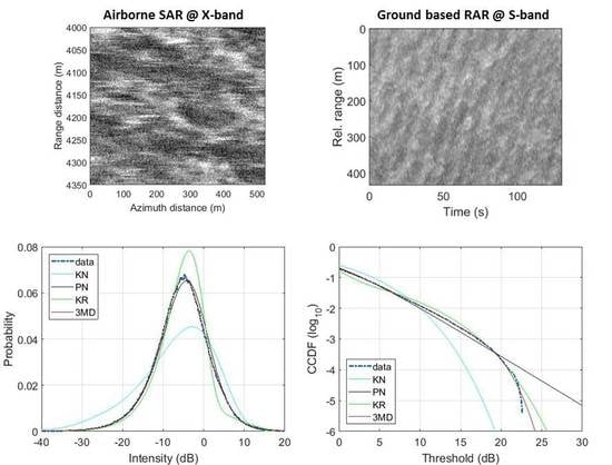
1. Introduction

In an operational context, radar sensors are a powerful tool for detecting targets in the maritime environment as they can be used at any time of day and in almost any weather condition [1]. They typically operate with an electromagnetic frequency between 1 and 15 GHz by exploiting the fact that man-made targets scatter with a higher energy compared to the surrounding sea. Maritime surveillance radars typically operate at low grazing angles where the mean power of the sea clutter is smallest. However, sea clutter collected from this geometry also contains many “sea-spikes” which manifest as undesired strong returns and are often the cause of false detections [2]. This is due to the scattering caused by discrete returns and breaking waves/whitecaps, which are worse when a swell is present [3], or when the radar has a high range resolution and/or horizontal polarization [4].

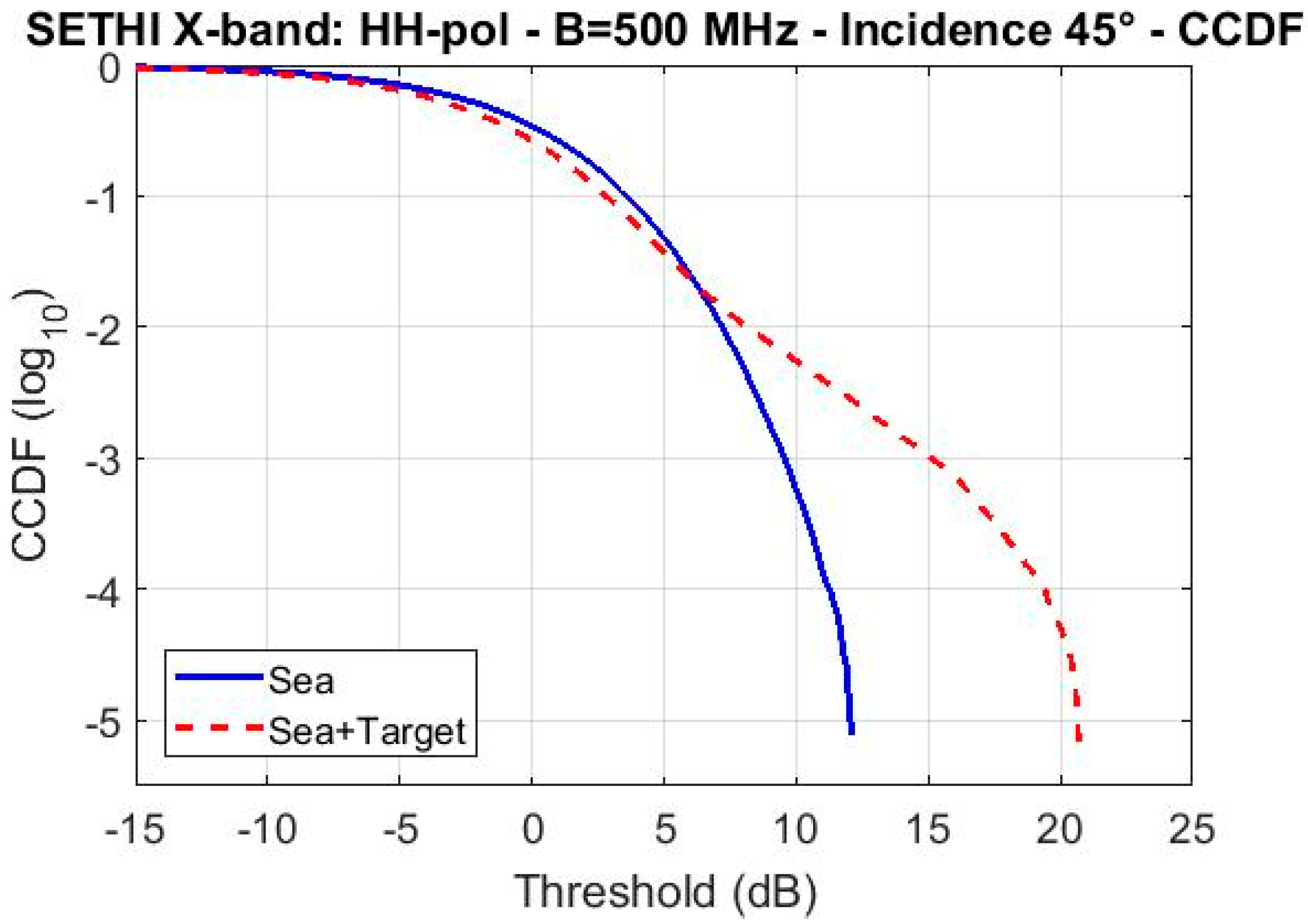
Many detection methods have been published in the literature, for a review the reader is referred to [1] and [5]. They work by comparing the average value of the backscattered signal with a reference value estimated over a target-free area. Due to the randomness and the spatial variability of the sea clutter, a reasonable sized data region must be used to provide an accurate estimate of the amplitude statistics and enable the detection of targets with low reflectivity. Consider the synthetic aperture radar (SAR) image shown in Figure 1 which was collected by SETHI [6], the airborne remote sensing radar developed by ONERA (see Section 4.3). The statistics of the backscattered signal were computed over a target-free sea surface (blue box) and over an area containing a ship (red box). By visualizing the complementary cumulative distribution function (CCDF), Figure 2 highlights the impact of the target on the signal statistics. A strong deviation is shown in the tail of the distribution, compared to that obtained when no target is present.

Target detection is typically approached with a constant false alarm rate (CFAR) scheme [1,3] and the selection of a threshold which limits the number of false alarms, while maintaining a desired probability of detection. This can be achieved by fitting a theoretical amplitude distribution or probability density function (PDF) to the target-free radar backscatter. This also allows for much lower false alarm rates to be used when there is insufficient data. Also, the presence of a maritime target usually manifests itself in the tail of the radar distribution due to its higher amplitude return.

There has been a long development of PDF models used to fit both real aperture radar and SAR. With coarse range resolution, a reasonable model for the sea-clutter PDF is the Rayleigh distribution [7]. As the range resolution becomes finer, the variation of the sea swell is better resolved and the effect of sea-spikes becomes more pronounced. From a statistical point-of-view, sea-spikes produce a non-Gaussian ‘long’-tailed, or ‘spiky’ distribution [4,7]. These radar returns have a larger magnitude which has led to the development of PDF models with longer tails such as the log-normal [8] and Weibull [9] distributions. A popular and widely used framework for developing PDF models is the compound Gaussian model which was originally proposed for use in sea-clutter by Ward [3]. This model includes a temporal or fast varying component known as speckle which relates to the Bragg scattering (Bragg scattering occurs when the radar wavelength is resonant with the sea wave), and a slowly varying component which captures the underlying swell and models the texture. The most popular compound model in the literature is the K distribution [3,10,11] and its extended version which accounts for the radar instrument noise, namely the K+Noise [3]. Similarly, the Pareto distribution [12,13] and its extended version, the Pareto+Noise [14] has become popular due to its ability to model the extended tail of the amplitude distribution. In this paper, we consider these distributions as well as two others proposed in the literature, the K+Rayleigh [15,16] and the 3MD distributions [17]. The latter distribution has demonstrated great potential for modeling SAR sea-clutter and is unique in the way it models the sea clutter texture as a combination of discrete components.

While there are many studies in the literature looking at the suitability of PDF models to represent radar sea clutter, few contain a quantitative evaluation of the accuracy in fitting the amplitude distribution. The main contribution of this paper is an analysis of the most recent and effective theoretical models for modeling non-Gaussian distributed sea clutter. This is achieved using fine resolution datasets from a ground based bistatic radar and two airborne radars operating at different frequency bands (L-, S-, and X-band), and covering a wide range of sea states and geometries. This builds on the earlier study in [11] by expanding the range of measurement configurations and amplitude distribution models. To assess performance, two metrics are used to quantitatively evaluate the ability for each model to represent the sea clutter amplitude distribution.

The paper is organized as follows: Section 2 describes the goodness of fit metrics, Section 3 summarizes the theoretical distributions, and Section 4 describes the data sets. Section 5 then summarizes the results and concludes by identifying the most suitable distribution to model the sea clutter.

2. Measures of Goodness of Fit

The aim of this paper is to evaluate the accuracy of different PDF models for modeling radar sea clutter. To quantitatively measure how well a model fits actual observations, there are many statistical tests in the literature [11]. In this paper, we focus on two goodness of fit measures: the Bhattacharyya distance (BD) and the threshold error. These metrics will be measured for the three radar datasets covering a wide variety of wind speeds, collection geometries, frequencies, and polarizations.

2.1. The Bhattacharyya Distance

The Bhattacharyya distance is a metric which varies between 0 and infinity [18]. It measures the similarity between the theoretical PDF P(.) and the actual data distribution Q(.) computed over the same data samples, $x_k$. The Bhattacharyya distance is commonly used to evaluate the accuracy of statistical distributions to represent experimental data.

$$\begin{array}{cc}BD=-\ln \left({\displaystyle \sum _{x_k}}\sqrt{P\left(x_k\right)Q\left(x_k\right)}\right)& 0\le BD\le \infty \end{array}$$

(1)

The smaller the Bhattacharyya distance, the better the goodness of fit and thus the accuracy of the model to represent the radar sea clutter.

2.2. Threshold Error

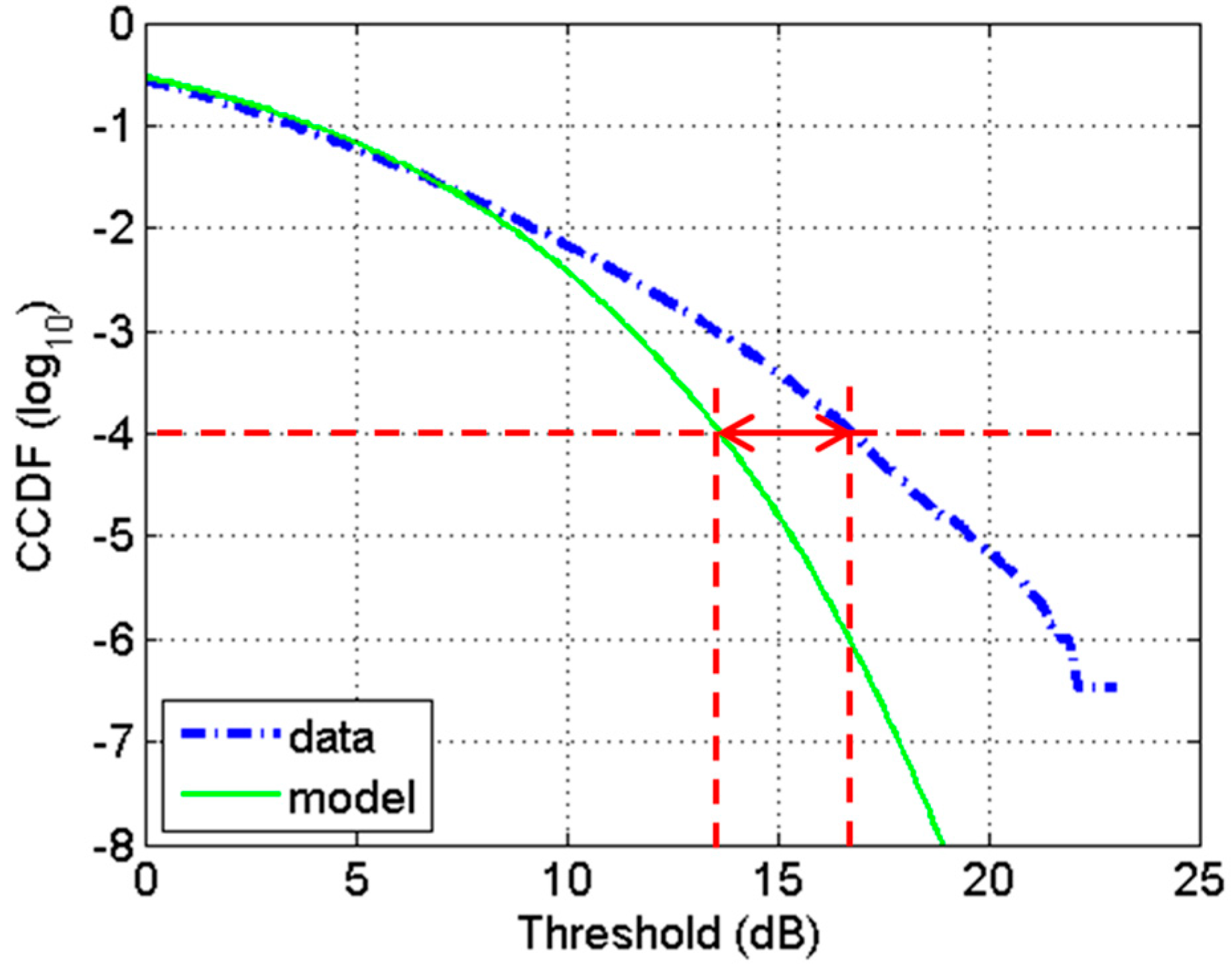
The second metric is the threshold error which is determined by first calculating the CCDF for both the empirical data and the proposed model. The threshold error is then the difference between the two results at a fixed CCDF value, often 10⁻⁴ or lower, depending on operational requirements [19]. The CCDF is important due to its relationship with the threshold in a detection scheme used for distinguishing between targets and interference. In this context, it is commonly referred to as the probability of false alarm. This measure is illustrated in Figure 3 for a CCDF of 10⁻⁴ (see red arrows). The threshold error is computed on the x-axis by measuring the difference between the actual CCDF (blue line) and the modeled CCDF (green line). The smaller this gap, the better the goodness of fit between the data and the model. This is a useful practical metric as it defines how far over or under estimated a CFAR threshold would be set when the distribution of the sea clutter is incorrectly estimated.

3. Amplitude Distribution Models

In this section, we outline the four distributions used for our analysis: K+noise, Pareto+Noise, K+Rayleigh and 3MD. As these are all compound distributions, we start by outlining the development of such models. Consider a radar receiving in-phase and quadrature data from an external clutter source with its amplitude defined by Gaussian statistics with zero mean and variance, x. In addition, instrument noise from the radar will add a component $p_n$ which is included by offsetting the variance x.

In target detection analysis, the envelope of the received pulses is often converted to power (square law) and the clutter distribution becomes exponential. This component is known as speckle in the compound representation. For a frequency agile or scanning radar with sufficient time between looks, a common method to improve the detection performance is to sum a number of looks. If there are M independent exponential random variables, $z={{\displaystyle \sum }}_{m=1}^M{y}_m$, then the received power is described by a gamma PDF,

$$P\left(z|x\right)=\frac{z^{M-1}}{{\left(x+{\sigma }_n^2\right)}^M\Gamma \left(M\right)}\exp \left[-\frac{z}{x+{\sigma }_n^2}\right]$$

(2)

where $0\le x\le \infty ,$ Γ(.) is the gamma function and ${\sigma }_n^2$ is the instrument noise power. In order to include the texture component which modulates the speckle, we integrate over the speckle mean,

$$P\left(z\right)={{\displaystyle \int }}_0^{\infty }P\left(z|x\right)P\left(x\right)dx$$

(3)

where P(x) is the distribution of the texture component. While there are analytic solutions in many cases, when instrument noise is included in the model, numerical integration must be used to evaluate the compound distribution. In the following, only single-look intensity data is considered with the data represented in decibels (dBs).

The parameters of the K+Noise, Pareto+Noise, and K+Rayleigh distributions are estimated using the zlogz method which has demonstrated the best tradeoff for accuracy and computational efficiency [20]. However, for the 3MD distribution, there is no suitable zlogz estimator and the model parameters are estimated using a least squares minimization between the CCDF of the data and the model. This is a more computationally intensive parameter estimation approach. To quantify the difference in run time, 100 iterations were performed and the run times averaged. For the K+Noise, Pareto+Noise, and K+Rayleigh zlogz estimators, the mean run times were 0.13, 0.12, and 0.13 s respectively, while for the 3MD least squares minimization, the mean run time was 1.57 s, which is approximately 12 times longer than the zlogz estimators.

3.1. K+Noise Distribution

The K+Noise (KN) distribution is a well-established model for representing high-resolution radar sea clutter [3,7]. It is a continuous mixture of an exponential or gamma distribution for the uncorrelated speckle intensity (fast temporal variation) with a gamma distribution for the clutter mean power (slow spatial variation) [3,21],

$$P\left(x\right)=\frac{b^{\nu }}{\Gamma \left(\nu \right)}{x}^{\nu -1}\exp \left[-bx\right]$$

(4)

where $\nu$ > 0 and $b=\nu /p_c$ are the shape and scale parameters respectively and $p_c$ is the mean clutter power. In the absence of instrument noise, $p_n=0$ and the solution to (3) is given by

$$P\left(z\right)=\frac{2{\left(bz\right)}^{\frac{\nu +M}{2}}}{z\Gamma \left(\nu \right)\Gamma \left(M\right)}{K}_{\nu -M}\left(2\sqrt{bz}\right)$$

(5)

where $K_{\nu -M}(.)$ is the modified Bessel function of the second kind with order ν − M. The zlogz estimator for the shape is found by numerically solving the following equation for $\hat{\nu }$ [20],

$$\frac{E\left(z\log z\right)}{E\left(z\right)}-E\left(\log z\right)-\frac{1}{M}=\frac{1}{1+1/C}{e}^{\widehat{\nu }/C}{G}_{\widehat{\nu }+1}\left(\widehat{\nu }/C\right)$$

(6)

where E(.) is the statistical mean or expectation operator, C is the clutter to noise ratio (CNR) and G(.) is the generalized exponential integral function [20].

3.2. Pareto+Noise Distribution

The Pareto+Noise (PN) distribution is another popular compound distribution used to model the sea-clutter backscatter [14]. It is formed with an inverse gamma distribution for the texture

$$P\left(x\right)=\frac{d^a}{\Gamma \left(a\right)}{x}^{-a-1}\exp \left[-d/x\right]$$

(7)

where $a$ and $d=p_c\left(a-1\right)$ are the shape and scale parameters respectively. Similar to the K+Noise distribution, there is no closed form expression unless the mean instrument noise power, $p_n=0$. In this case, the Pareto distribution is given by

$$P\left(z\right)=\frac{z^{M-1}{d}^a\Gamma \left(M+a\right)}{{\left(d+z\right)}^{M+a}\Gamma \left(\nu \right)\Gamma \left(M\right)}$$

(8)

For the Pareto+Noise distribution, the zlogz estimator for the shape is found by numerically solving the following equation for $\widehat{a}$ [20],

$$\frac{E\left(z\log z\right)}{E\left(z\right)}-E\left(\log z\right)-\frac{1}{M}=\frac{1}{1+\frac{1}{C}}\left(\frac{1}{\widehat{a}-1}-e^{\left(\widehat{a}-1\right)C}{G}_{\widehat{a}}(\left(\widehat{a}-1\right)C\right)$$

(9)

3.3. K+Rayleigh Distribution

The K+Rayleigh (KR) distribution is an extension to the KN model designed to capture any extra Rayleigh component in the data which arises from the non-Bragg scattering [16]. It explicitly separates the speckle mean level into two components, $x=x_r+p_r$, where $p_r$ is the power of the extra Rayleigh component. As with the KN model, the texture is given by a gamma distribution,

$$P\left(x_r\right)=\frac{b_r^{{\nu }_r}}{\Gamma \left({\nu }_r\right)}{x}_r^{{\nu }_r-1}\exp \left[-b{x}_r\right]$$

(10)

where ${\nu }_r>0$ and $b_r={\nu }_r/p_c$ are the shape and scale parameters respectively. The PDF of the KR distribution has no closed-form expression and is calculated by integrating (3) with respect to the modified speckle mean level, $x_r$ instead of the total speckle $x$. The influence of the extra Rayleigh component can be measured by the ratio of the mean of the Rayleigh component, $p_r$, to the mean of the gamma distributed component, $p_c$, of the clutter and is defined by

$$k_r=\frac{p_r}{p_c}$$

(11)

To estimate the KR parameters, the sum of the instrument noise power and Rayleigh power needs to be estimated in addition to the shape. This is achieved by first substituting the CNR in (6) with the clutter to noise plus Rayleigh power, $\widehat{C}$, using the following relationship for the distribution moments,

$$\widehat{C}=\frac{p_c}{p_r+p_n}=\frac{1}{\frac{1}{\sqrt{{\widehat{\nu }}_{r}r}}+1}$$

(12)

where

$$r=\frac{M}{M+1}\frac{E\left(z^2\right)}{E^2\left(z\right)}-1$$

(13)

and then solving the numerical relation in (6). The Rayleigh mean power can then be found by rearranging (12),

$$p_r=\frac{p_c}{\widehat{C}}-p_n$$

(14)

3.4. Tri-Modal Discrete Distribution

The compound models presented previously all assume a continuous texture distribution which suggests a small probability of infinite texture values. The motivation of the 3MD model is to instead use a discrete texture model that assumes the sea clutter consists of a finite number, I, of distinct modes or scatterer types [17]. This implies that the scatterers in the observed scene are realizations from homogeneous clutter random variables with different texture values. The PDF of the texture is given by

$$\begin{array}{ccc}P\left(x\right)={\displaystyle \sum _{n=1}^I}{c}_n\delta \left(x-a_n\right),& {\displaystyle \sum _{n=1}^I}{c}_n=1,& a_n,c_n>0\end{array}$$

(15)

$$\delta \left(A\right):=\{\begin{array}{ll}1& \mathrm{if}A=0\\ 0& \mathrm{otherwise}\end{array}$$

(16)

where $a=\left[a_1,\dots ,a_I\right]$ are the discrete intensity texture levels and $c=\left[c_1,\dots ,c_I\right]$ are the corresponding weightings. The resulting PDF after solving (3) is then given by

$$P\left(z\right)=\frac{M^M}{\Gamma \left(M\right)}{z}^{M-1}{\displaystyle \sum }_{n=1}^I{c}_n\frac{\exp \left(-\frac{Mz}{{\rho }_c{a}_n^2+{\rho }_n}\right)}{{\left({\rho }_c{a}_n^2+{\rho }_n\right)}^M}$$

(17)

with

$${\rho }_c+{\rho }_n=\frac{p_c}{p_c+p_n}+\frac{p_n}{p_c+p_n}=1$$

(18)

In their original work [17], the authors have reported that I = 3 modes are sufficient to accurately model high spatial resolution sea clutter data collected by spaceborne SAR sensors. One of the consequences of this discretization is that spatial and long-time correlation cannot be modeled as part of the texture, and hence the model is less suitable for clutter simulation. The 3MD distribution also requires the non-trivial estimation of $2I$ unknown parameters. This can be achieved with a least squares minimization between the 3MD model and data CCDF in the log domain. The fitting process first assumes a single mode ($I=1$). If the BD of that fit is greater than −30 dB, the parameters for a bi-modal fit ($I=2$) are then estimated. This is repeated up to the maximum number of modes, which is set to $I=5$ unless otherwise stated. The model components, $a_n$, are then ordered from largest to smallest and any modes where the weightings, $c_n<{10}^{-3}$ are removed. Note that the threshold value of BD = −30 dB comes from experimental observation below which there is little change in the 3MD distribution.

4. Radar Sea Clutter Datasets

Three sea clutter datasets are used in this paper to evaluate the accuracy of the proposed PDF models. These have been collected by different radar sensors operating at different frequency bands (L-, S-, and X-band), different platforms (airborne and ground-based) and covering a wide range of sea state and geometries. Two of the data sets are from a real beam radar, while the third comprises images formed from a synthetic aperture radar.

4.1. NetRAD Dataset: Ground Based Radar Sensor

The Netted Radar (NetRAD) is a ground-based coherent bistatic radar system operating at S-band (carrier frequency of 2.45 GHz) [22,23]. The system was developed jointly by the University College London, UK and the University of Cape Town, South Africa. It works in both monostatic and bistatic configurations with the two nodes synchronized in time with GPS disciplined oscillators over a 5 GHz wireless link. The system configuration used for gathering the data analyzed included a peak transmit power of 57.7 dBm, pulse repetition frequency (PRF) of 1 kHz, antenna gain of 23.8 dBi, and a bandwidth of 45 MHz providing a range resolution of 3.3 m. The antennas work with either vertical (V) or horizontal polarizations (H).

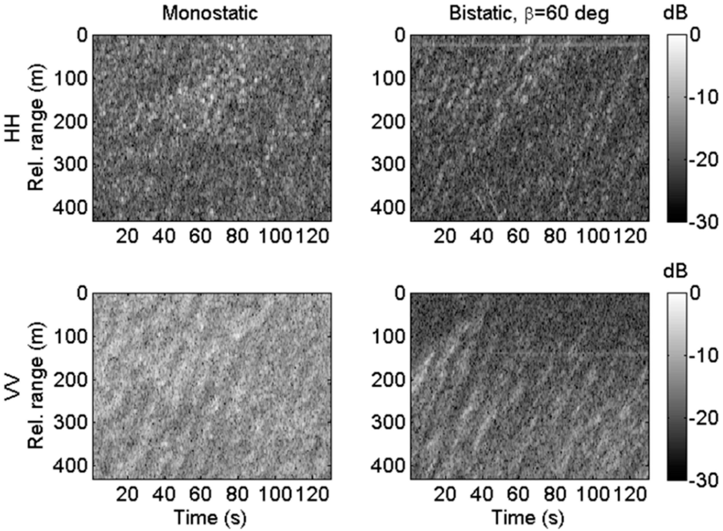
The data assessed here is summarized in

Table 1. Properties of the NetRAD radar sea clutter acquisitions investigated in this study.

Run	Frequency	Pol.	Bistatic Angle (°)	Wind Speed (m/s)	Wave Period (s)	Wave Direction (°)	Wave Height (m)
1	S-band	VV	60	10	7.1	289	3.3
2			90	10	7.7	279	3.5
3			120	11	8.3	270	3.7
4		HH	60	11	8.3	283	3.9
5			90	11	8.3	283	3.9
6			120	12	8.6	276	4.0

and was generated during a 2010 series of trials in South Africa near the Cape Point area. The baselines between each of two radar nodes and the illuminated area were 1830 m and in order to vary the bistatic angle, the antennas were rotated to cover different regions of the sea. The grazing angles from the geometries varied from 0.6° to 1.5° [23], which will have a minor impact on the backscattered signal compared to changes with the polarization or the bistatic angle. In the following analysis, 10 s of data have been used for each run, resulting in more than 10⁶ samples. Wind and wave information is given in Table 1 and was obtained from the Cape Point wave buoy, approximately 7 km from the trial location. In Figure 4, an example of the monostatic and bistatic radar data is displayed for a bistatic angle of 60°.

4.2. INGARA Dataset: Airborne Radar Sensor

INGARA is a polarimetric radar system maintained and operated within the Defence Science and Technology Group in Australia [24]. During the ocean backscatter collections in 2004 and 2006, the sea clutter data was collected at X-band (10.1 GHz carrier frequency) with a 200 MHz bandwidth giving a 0.75 m range resolution. Alternate pulses transmitted horizontal and vertical polarizations resulting in a nominal PRF of 300 Hz. The radar was operated in a circular spotlight-mode covering 360° of azimuth angles and each day, the radar platform performed at least six full orbits around the same patch of ocean to cover a large portion of grazing angles between 15° and 45°.

During the trials at sea, the wind and wave information was collected using DST Group’s wave buoy, which was located within 50 km of the imaging site. Wind data from several different sources were collected and compared during the trials. For the 2004 trial, the most reliable wind data were obtained from the Bureau of Meteorology automatic weather station located on a cliff top about 50 km northeast of the wave buoy deployment site. Hence, it will be subjected to some error and, possibly a time delay compared with the actual conditions at the wave buoy site. For the 2006 trial, the most reliable wind data were made with a handheld anemometer on a boat near the imaging area.

Table 2. Properties of the INGARA radar sea clutter acquisitions investigated in this study.

Run	Frequency	Pol.	Wind Direction (°)	Wind Speed (m/s)	Wave Period (s)	Wave Direction (°)	Wave Height (m)
1	X-band	Quad-pol	248	10.2	12.3	220	4.9
2			248	7.9	11.8	205	3.5
3			315	10.3	10.4	210	2.6
4			0	13.6	8.8	293	3.2
5			68	9.3	9.7	169	2.5
6			315	9.5	11.4	234	3.0
7			22	13.2	12.2	254	3.8
8			0	8.5	12.5	243	4.3
9			115	8.5	3.1	112	0.62
10			66	3.6	2.6	35	0.25
11			83	3.5	4.0	46	0.41
12			124	10.2	4.6	128	1.21

shows the sea conditions over the two data collections, with Runs 1–8 from the 2004 collection and Runs 9–12 from 2006. The data analyzed in this paper has been pooled into blocks of 5° azimuth and 3° grazing with each block containing approximately 10⁶ samples. An example of the data is shown in Figure 5 for the downwind direction and 30° grazing.

4.3. SETHI Dataset: Airborne Imaging Radar Sensor

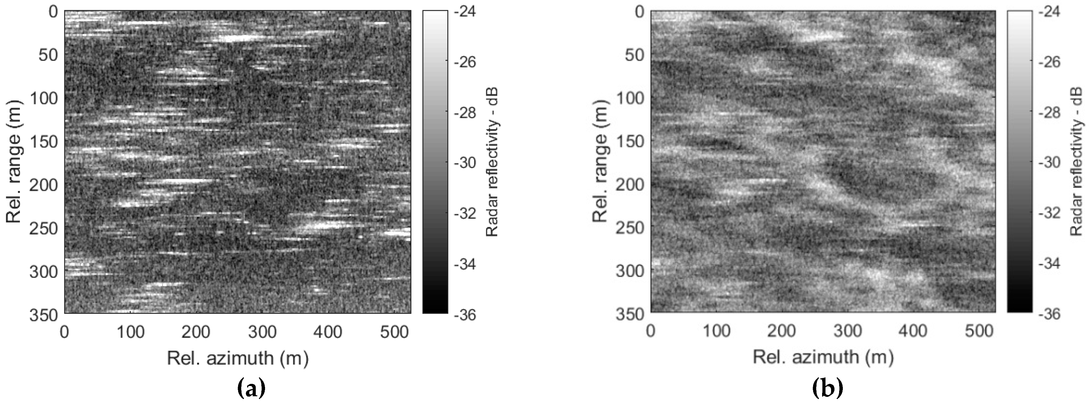
SETHI is the airborne remote sensing radar developed by ONERA [6]. It is a pod-based multi-frequency high resolution SAR system designed to explore the scientific applications of remote sensing. Both L- and X-band SAR data have been collected at two different geographical positions, the Atlantic ocean and the Mediteranean sea along the French coast. The bandwidths are 300 MHz at X-band (9.6–9.9 GHz) and 150 MHz at L-band (1.25–1.4 GHz). The data presented in this paper is described in

Table 3. Properties of the SETHI data sets. Both the range and azimuth spatial resolutions are equal.

Run	Frequency	Pol.	Area	Spatial Res. (m)	Grazing Angle (°)	Wind Speed (m/s)	Wave Height (m/s)
1	X-band	Dual-pol	Atl.	0.5	10	17.65	4.9
2				0.5	20	17.65	4.9
3				0.5	10	7.2	3.3
4				0.5	20	7.2	3.3
5				0.5	30	7.2	3.3
6	X-band	Dual-pol		0.5	20	10.2	3.6
	L-band			1
7	X-band	Dual-pol		0.5	10	10.1	3.6
8	X-band	Quad-pol	Med.	0.5	45	8.5	1.1
	L-band			1

and covers grazing angles from 10° to 45°, different sea states (significant wave heights from 1.1 to 4.9 m), a range of azimuth angles and either dual-polarized (HH, VV) or quad-polarized (HH, HV, VH, VV) antenna combinations. The flying trajectory was either linear (stripmap mode) or circular (spotlight mode) and the wind and wave information given in Table 3 was obtained from Météo-France, the French national meteorological service. An illustration of the X-band dual-pol SAR data at 10° grazing is given in Figure 6 (Run 3) where the horizontal and vertical axes correspond to the along-track (azimuth) and across-track (range) directions. Strong differences in radar responses can be seen as a function of the polarization state: the HH backscattered signal (Figure 6a) is strongly affected by sea-spikes (e.g., breaking waves), while the VV signal (Figure 6b) is dominated by short scale waves [25].

5. Results and Discussions

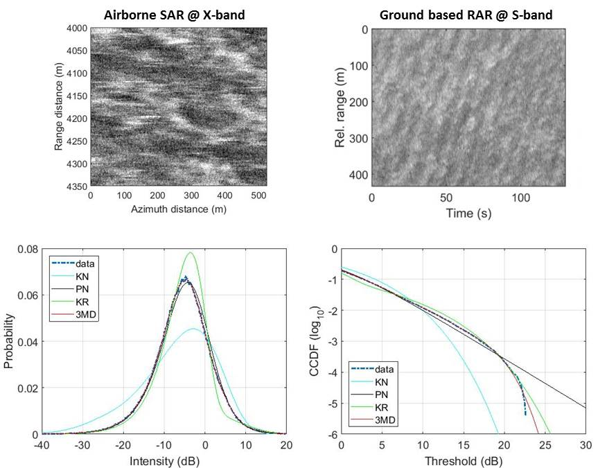
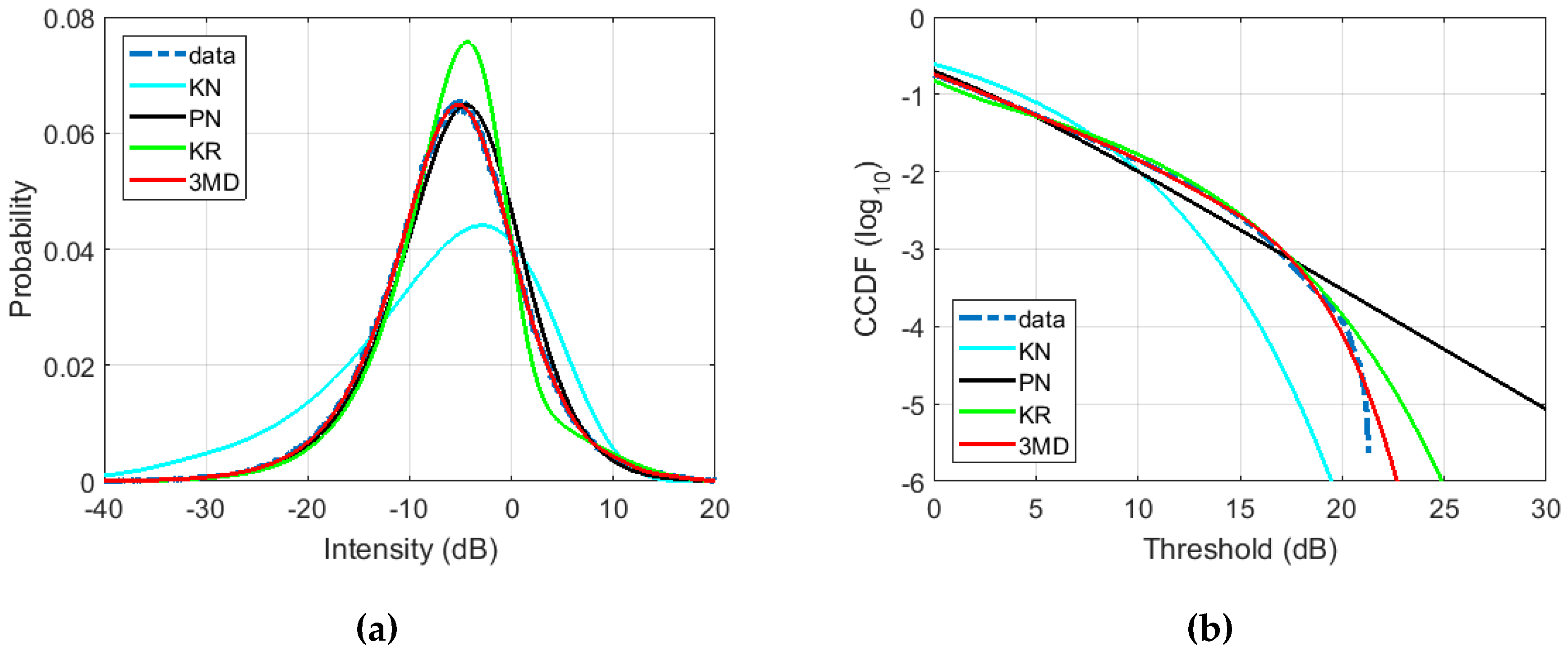
This section provides an analysis of the four amplitude PDF models applied to the NetRAD, INGARA, and SETHI datasets. For each result, the data is plotted in a thick blue dotted line, while the cyan, black, green, and red lines are for the K+Noise (KN), Pareto+Noise (PN), K+Rayleigh (KR), and 3MD models respectively. The PDF curves represent the probability of occurrence of radar intensity values (in dBs), while the CCDF curves show the probability that the radar intensity takes a value greather than the threshold (see Section 2.2). Both the Bhattacharyya distance and the threshold errors are provided for each example and reported in dBs.

5.1. NetRAD Analysis

In this section, we investigate the accuracy of the theoretical models to represent the NetRAD bi-static dataset. We first show an example of the model fits and report on the number of modes required by the 3MD model. We then study the model accuracy using the goodness of fit metrics, focusing firstly on the overall PDF fit and then the tail of the distribution.

The example in Figure 7 shows the results for Run 4 of the NetRAD bistatic data which has HH polarization and a bistatic angle of 60°. For this result, the 3MD model has been fitted to the data with $I=5$ modes. The parameter estimates are given in

Table 4. Parameter estimates for the models in Figure 7.

CNR (dB)	28.9
KN shape	0.58
PN shape	1.6
K+Rayleigh shape	0.04
K+Rayleigh kr—value	0.41
3MD mode 1 (a, c)	(0.458, 0.379)
3MD mode 2 (a, c)	(0.682, 0.345)
3MD mode 3 (a, c)	(1.163, 0.220)
3MD mode 4 (a, c)	(2.334, 0.0488)
3MD mode 5 (a, c)	(5.463, 0.0064)

, while the BD and threshold error results are given in

Table 5. Goodness of fit metrics for the models in Figure 7. Threshold error is measured at a CCDF of 10⁻⁴.

	BD (dB)	Threshold Error (dB)
KN	−15.65	5.17
PN	−31.55	−1.73
KR	−22.75	−0.02
3MD	−37.31	0.11

. For the KN and KR distributions we observe a strong mismatch in the body of the distribution (Figure 7a) with high BD values (Table 5), while the PN and 3MD models fit the data closely over all intensity values. However, the CCDF fits in Figure 7b clearly shows that the KN and the PN distributions both have a mismatch in modeling the distribution by under and over estimating the tail respectively, while the 3MD and the KR both match closely. This is reflected in the threshold error values in Table 5.

5.1.1. Number of Modes Required for the 3MD Distribution

In previous work, it has been reported that three modes are sufficient to accurately model amplitude distributions from spaceborne SAR data [17], airborne SETHI SAR data, and airborne INGARA real aperture sea clutter data [26]. We now investigate how many modes of the 3MD distribution are required to accurately model the mono and bistatic sea clutter from the NetRAD dataset.

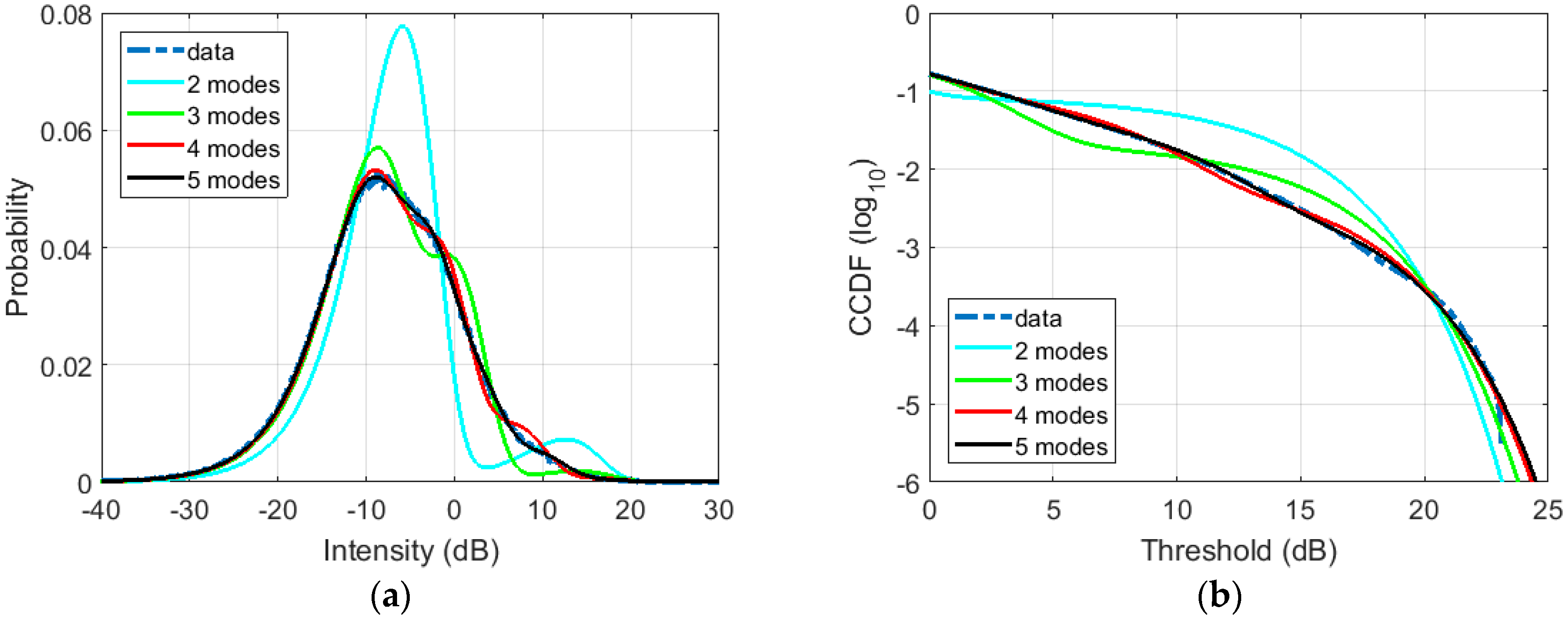
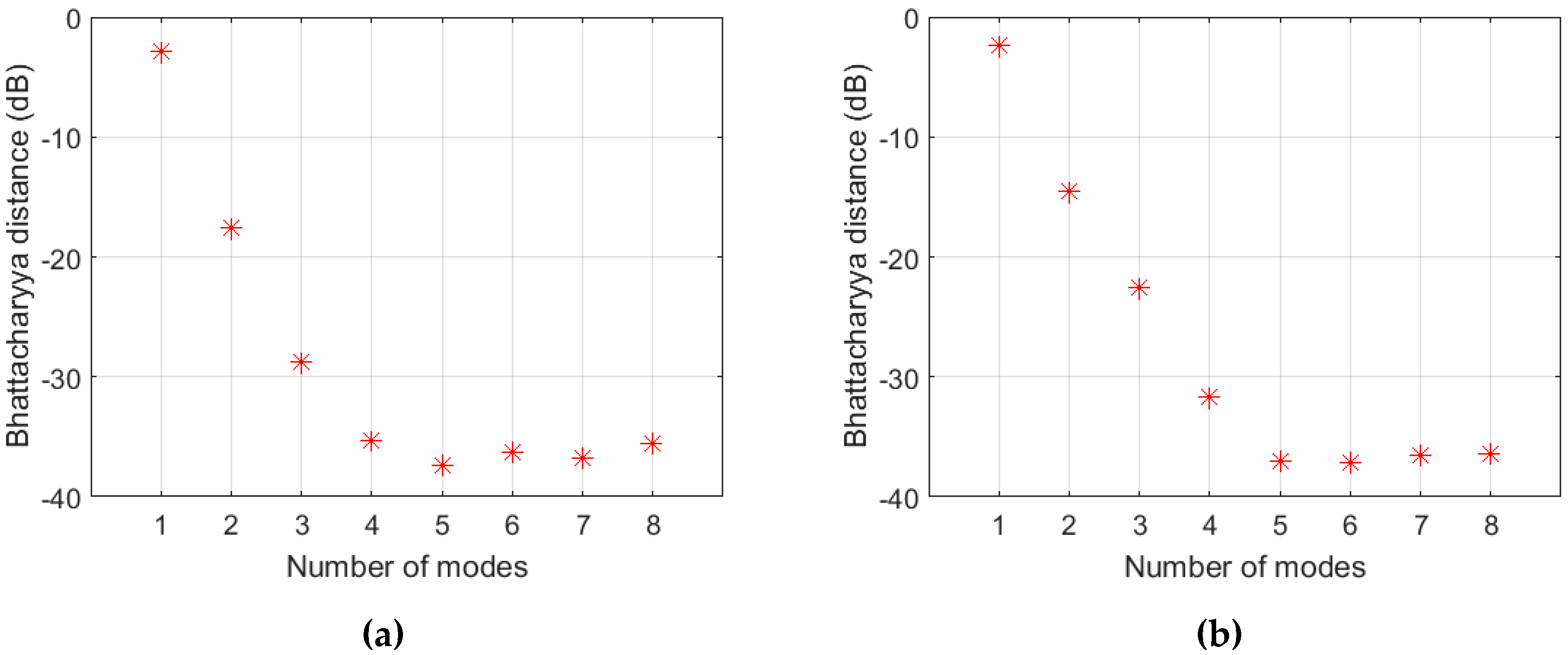
As discussed in Section 3.4, the minimum number of modes required for a good fit is determined when the BD goes below the desired value of −30 dB. Figure 8 shows an example model fit from the NetRAD bistatic data with 60° bistatic angle and VV polarization (Run 1) with different numbers of components, I. The BD for both polarizations is then shown in Figure 9 where we observe that four modes are required to satisfy the condition that the BD is less than −30 dB.

Table 6. 3MD distribution: minimum number of modes required to accurately match the NetRAD data.

Bistatic Angle	Polarization
	HH		VV
	Monostatic	Bistatic	Monostatic	Bistatic
60	4	4	3	4
90	4	3	2	5
120	3	3	2	3

summarizes the minimum number of modes required by the NetRAD data. Among the 12 datasets (monostatic and bistatic), 7 need 2 or 3 modes (which is in agreement with [17,26]), but we find that 5 datasets need 4 or 5 modes. The link between the number of modes and the acquisition parameters are not obvious from the available data and further study is required to fully understand this relationship. Nevertheless, we have demonstrated that the 3MD distribution is able to accurately model the amplitude distribution of each of the NetRAD datasets, but at the cost of a greater number of parameters to estimate, 2I.

5.1.2. Analysis of Model Accuracy

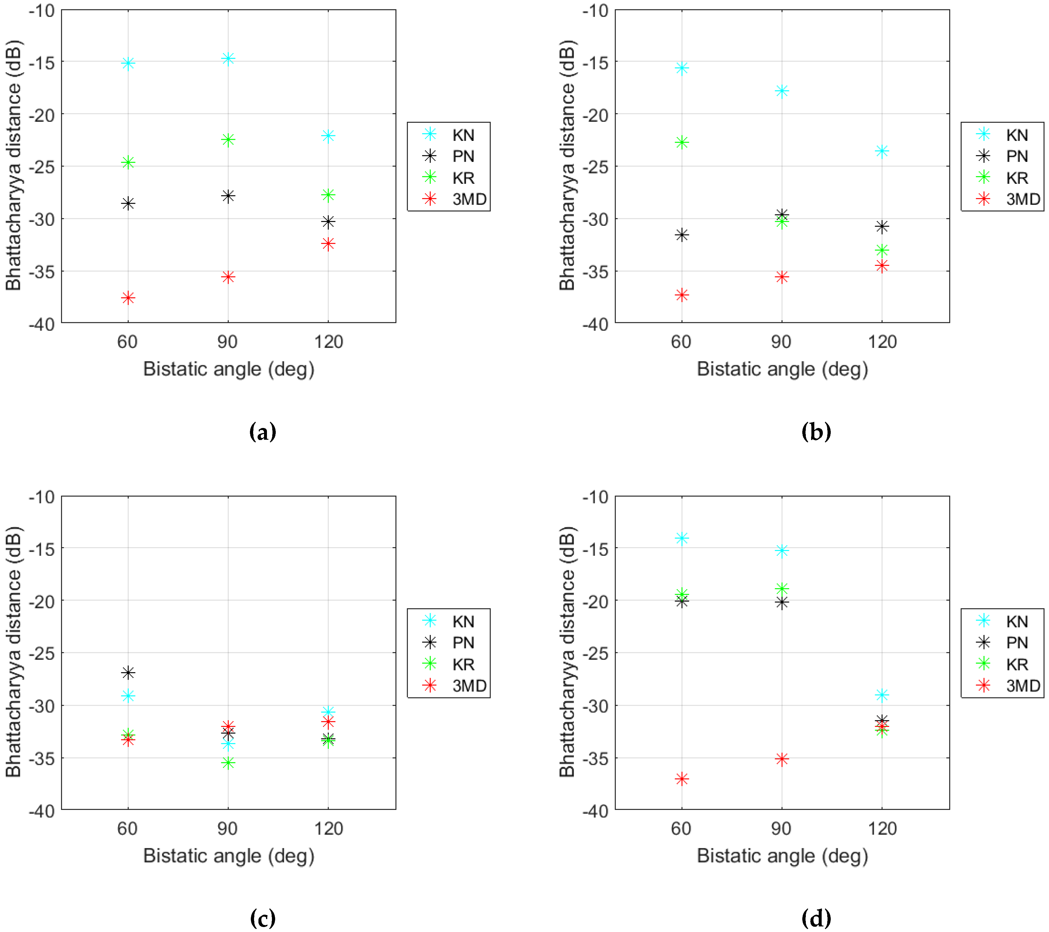
In this section we study the accuracy of the four models described in Section 3 when fitting amplitude distributions to the NetRAD dataset. Figure 10 first shows the BD for each bistatic angle and polarization. The only result that shows a good match for nearly every model (BD ≤ −30 dB) is the monostatic case with VV polarization (Figure 10c). However, it is only the 3MD distribution that has a consistently low BD over all the datasets. The other results are mixed with the PN and KR models both providing a good fit with some datasets, while mismatching with others (BD > −30 dB). The KN model nearly always fails to accurately fit the data.

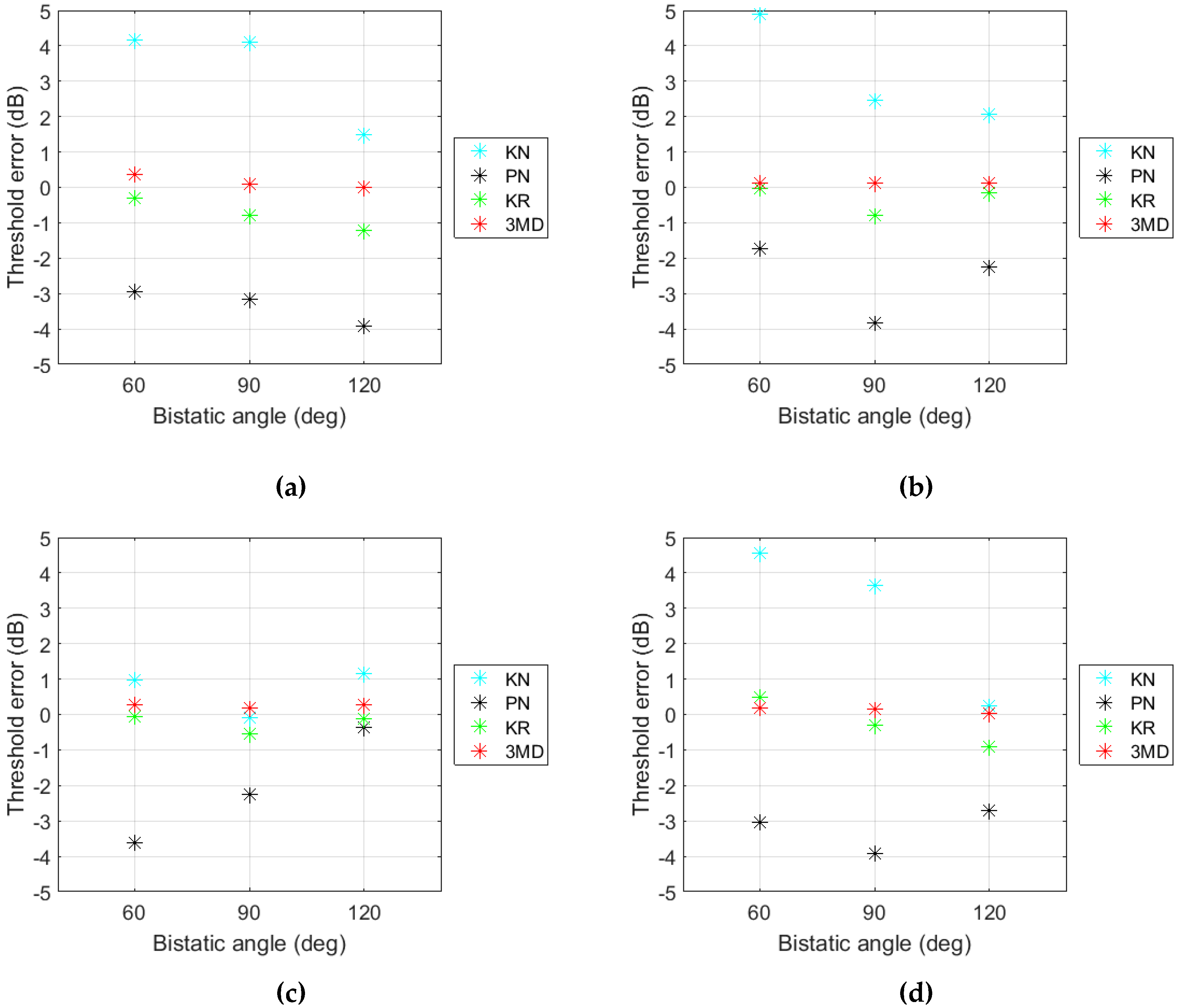
Results of the threshold error for a CCDF of 10⁻⁴ are then displayed in Figure 11, where low errors are observed for both the KR and 3MD models (<±1 dB), while the PN and KN distributions have a greater mismatch with errors up to ±4 dB. If the PN distribution was used in a detection scheme with such a large mismatch, there will be a large number of missed detections. Conversely, if the KN distribution were used, there would be a higher probability of false alarm.

5.1.3. Summary

Analysis of the NetRAD S-band monostatic and bistatic sea clutter dataset demonstrates that both the KN and PN distributions fail to match the data in many cases and would provide degraded detection performance if used in a detection scheme. However, the KR and 3MD distributions show a good match in the tail region, making them a good choice. When considering the total fit to both the body and distribution tail, it is only the 3MD model that is able to consistently provide good results, but at the cost of a higher number of parameters to be estimated.

5.2. Analysis of the INGARA Dataset

We now consider how the different distributions can model the INGARA sea clutter data set. Firstly, we give some illustrations of the proposed models with an example run. We then study the behavior of the texture for the 3MD model over a range of geometries. Finally, we look at the model accuracy for fitting each distribution to the INGARA dataset.

Two example datasets, Runs 3 and 9 are first considered with the respective sea conditions given in Table 2. Figure 12 shows the model fits for Run 3 in the upwind direction and 30° grazing. These results show the KN under fitting the HH polarization and the PN over fitting for each result. The KR model has a good fit until a CCDF value of 10⁻⁴, while the 3MD shows an excellent fit for all results. The estimated model parameters and goodness of fit metrics are given in

Table 7. Parameter estimates for the model fits in Figure 12.

Run 3	Polarization
	HH	HV	VV
CNR (dB)	11.7	6.5	21.6
KN shape	2.3	3.5	7.0
PN shape	3.4	4.7	8.0
K+Rayleigh shape	0.34	1.9	7.1
K+Rayleigh $k_r$—value	0.49	0.19	0
3MD mode 1 (a, c)	(0.70, 0.49)	(0.82, 0.74)	(0.82, 0.55)
3MD mode 2 (a, c)	(1.12, 0.47)	(1.42, 0.26)	(1.19, 0.45)
3MD mode 3 (a, c)	(2.11, 0.038)	-	-

and

Table 8. Goodness of fit metrics for the model fits in Figure 12. Threshold error is measured at a CCDF of 10⁻⁴.

	BD (dB)			Threshold Error (dB)
	HH	HV	VV	HH	HV	VV
KN	−30.7	−36.5	−36.0	1.6	0.2	−0.3
PN	−36.1	−35.1	−34.9	−0.8	−1.1	−0.9
KR	−35.1	−36.6	−36.0	−0.2	−0.1	−0.3
3MD	−36.5	−35.0	−36.0	0.1	0.2	0.1

respectively.

5.2.1. Parameter Variation for the 3MD Distribution

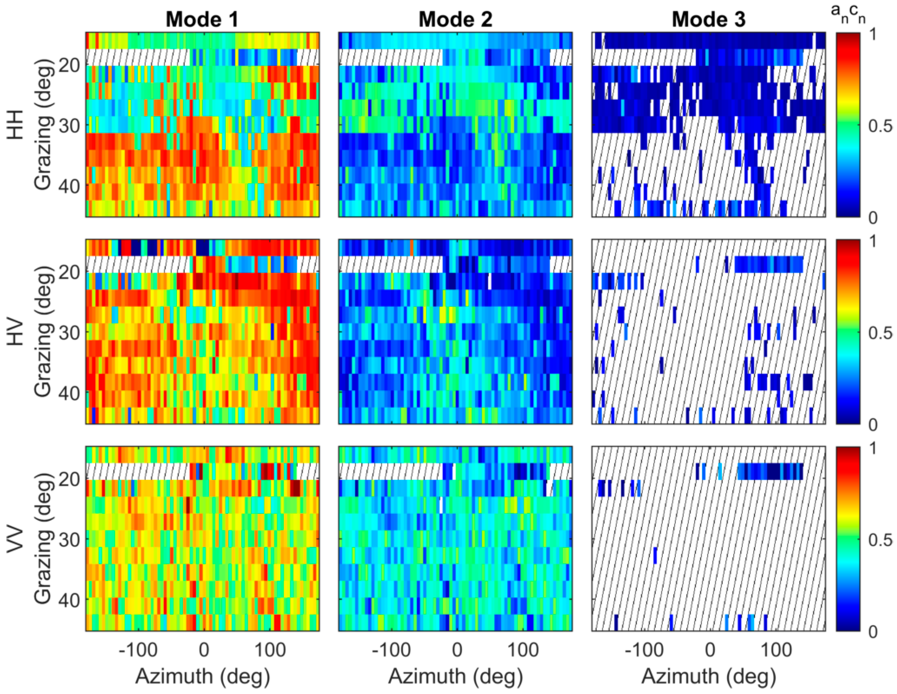
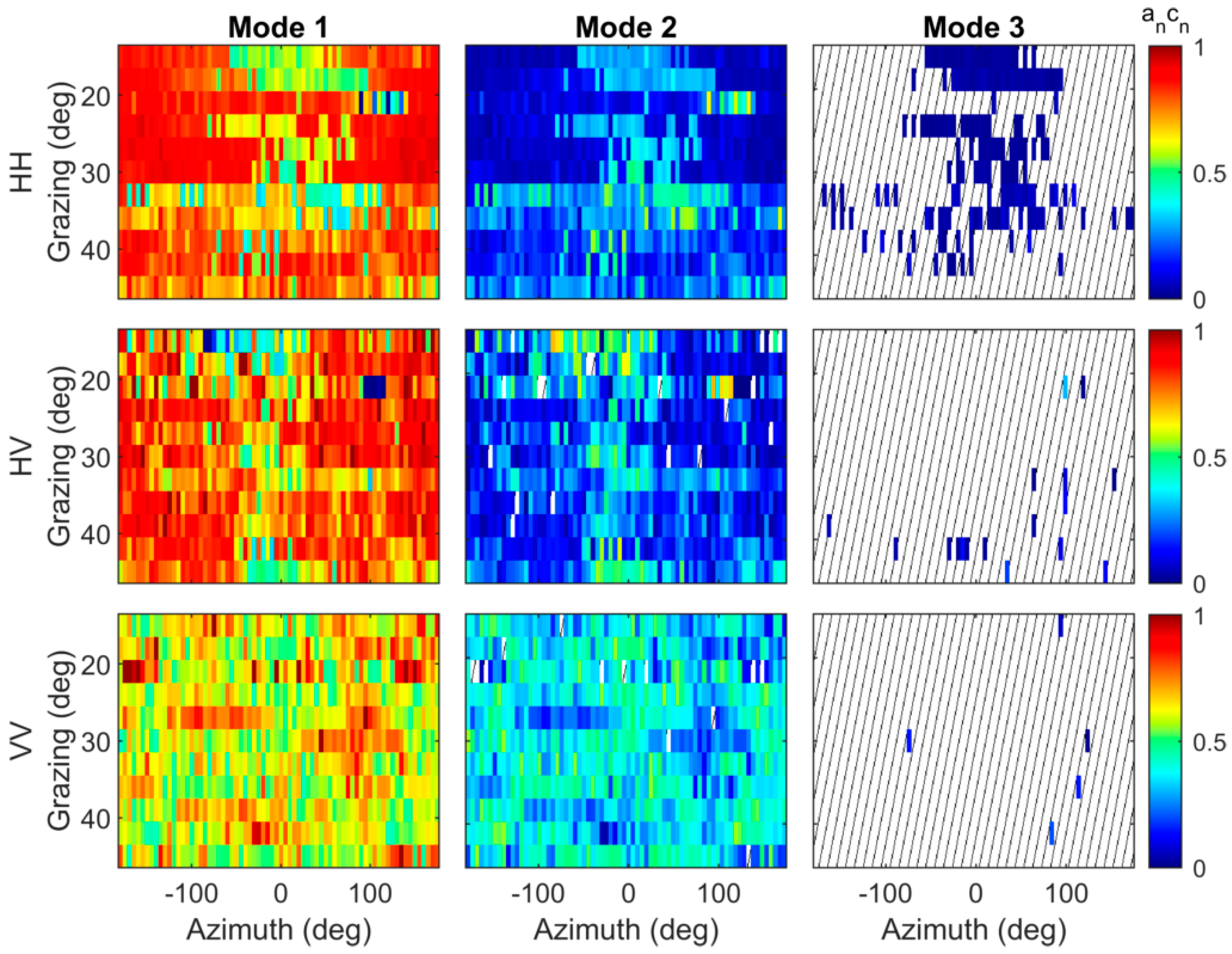
In order to further study the modes of the 3MD model, we compare the product of the texture locations $a_n$ and the proportion $c_n$ [17]. For INGARA Runs 3 and 9, Figure 13 and Figure 14 show this result for each polarization, over all azimuth angles and grazing angles from 15° to 45°. The dashed lines indicate either missing data or regions where no mode was required for the model fit. To achieve a BD lower than −30 dB, at least two modes were required for each polarization, with 53% and 20% of the HH data blocks requiring three. These latter data blocks are primarily in the low grazing angle region in the HH polarization where there is an even proportion spread between the first two modes ($a_n{c}_n~0.5$). Although not shown here, this result matches where the KR shape value is lowest indicating the spikiest clutter [26].

5.2.2. Analysis of Model Accuracy

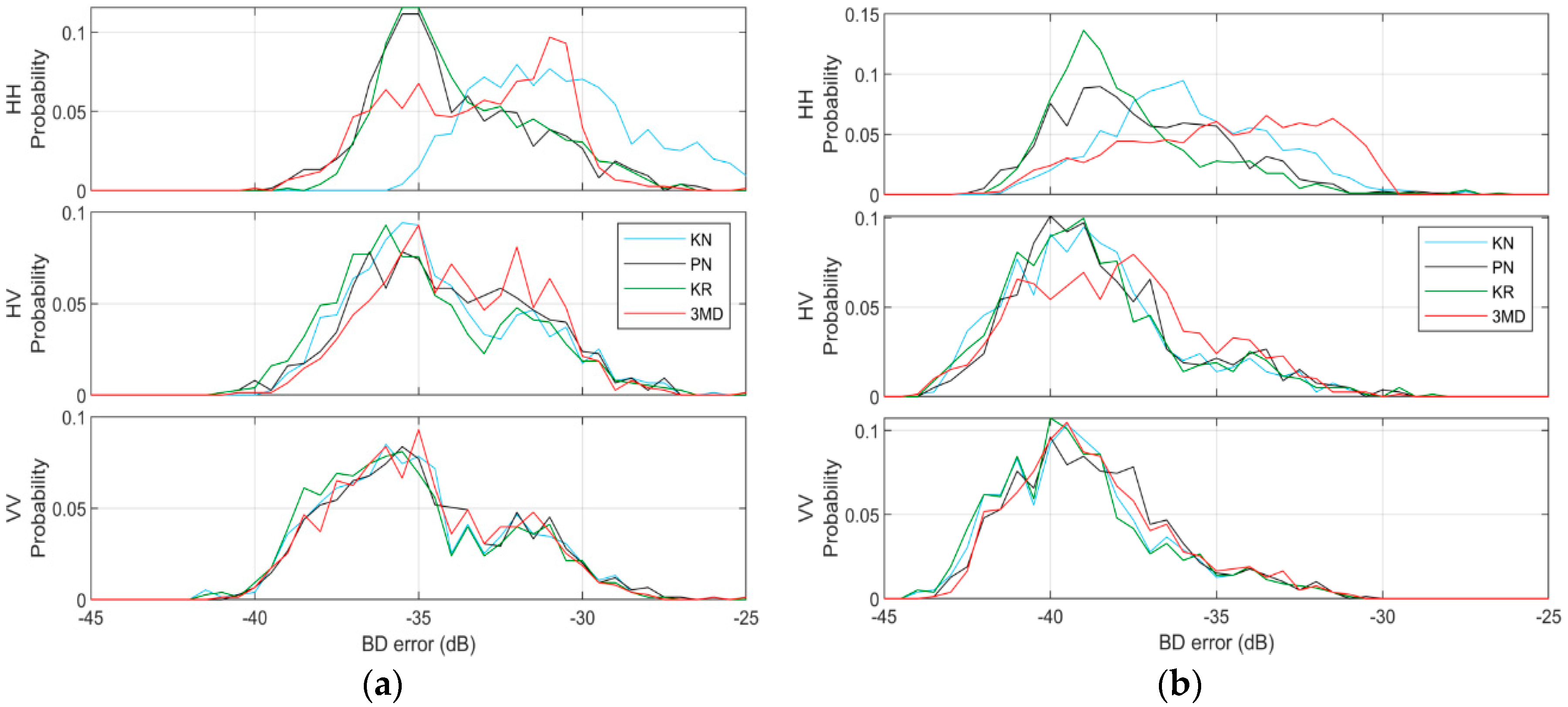
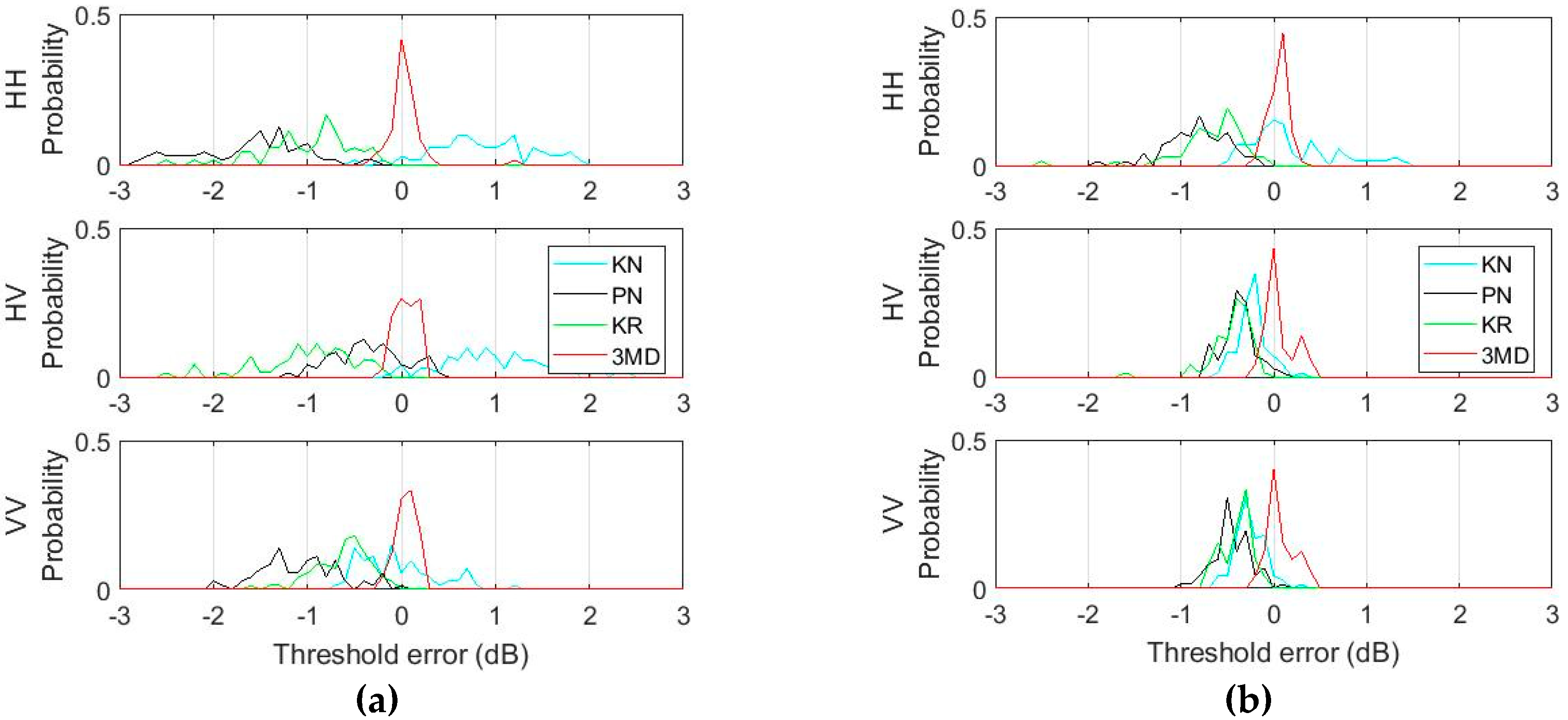
To determine the accuracy of the model fits over the two data runs, the BD and threshold errors at a CCDF value of 10⁻⁴ have been measured for all data blocks with the results shown as histograms in Figure 15 and Figure 16. For the BD, the biggest variation is seen for the HH polarization with the KN distribution having the highest value (worst fit) for Run 3 followed closely by the 3MD distribution. Note that the BD values for the 3MD distribution are nearly always less than −30 dB which is our stopping criteria for the model fit. The other two distributions, KR and PN have very similar results spread between −40 to −30 dB.

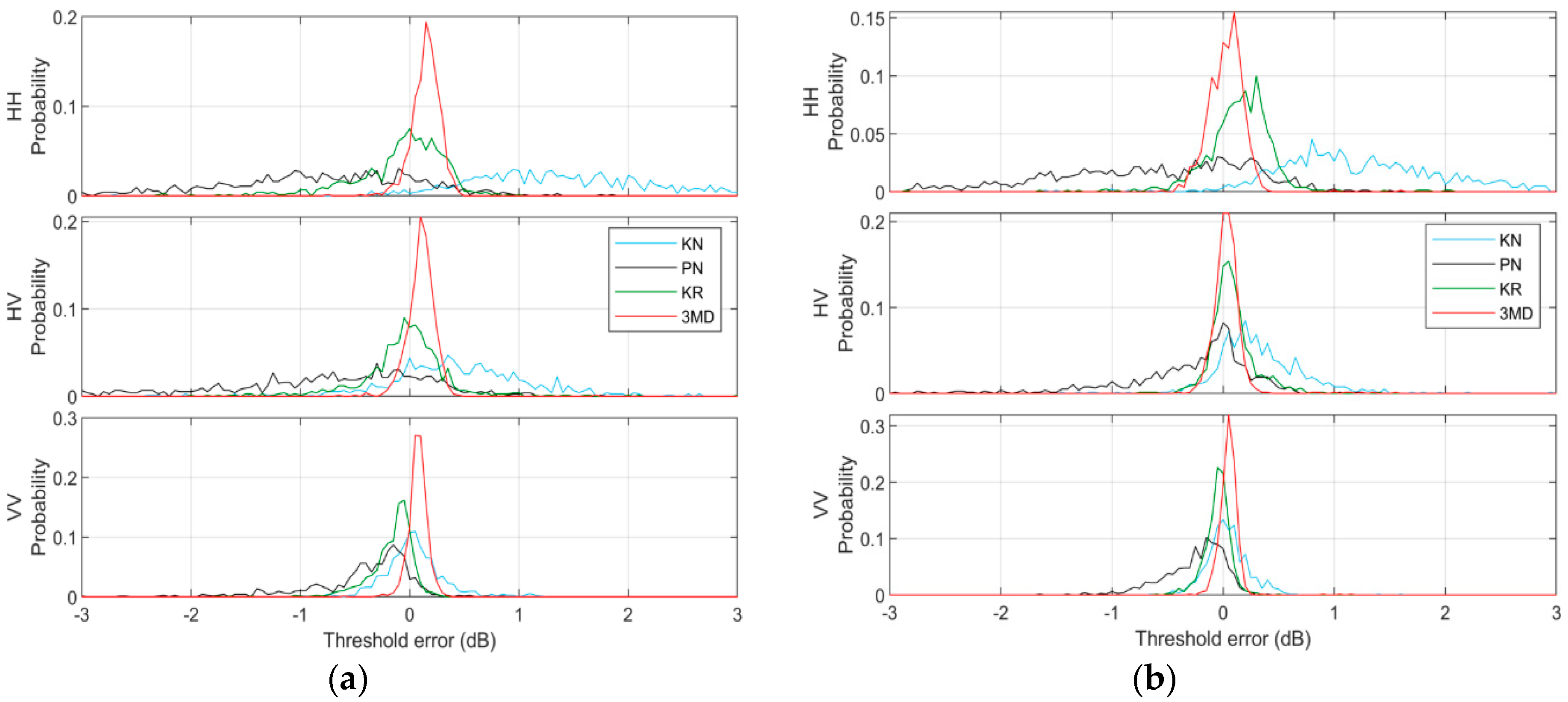
For the threshold error in Figure 16, the 3MD distribution clearly has the lowest error with very little bias around 0 dB. The KR distribution also has a low error spread, while the KN and PN show a wide range of threshold errors. Figure 17 then shows the threshold errors over the 12 different days/wind speeds in the upwind direction for grazing angles of 15°, 30°, and 45°. The same spread of errors are observed here with a large mismatch for the KN and PN distributions with mean absolute values of 0.76 and 0.89 dB respectively, while the KR and 3MD models show the lowest absolute mean errors of 0.30 and 0.11 dB. The largest errors were observed within the HH polarization at the lowest grazing angles for the PN and KN models, while data from the VV polarization showed a significantly reduced threshold error across all grazing angles.

5.2.3. Summary

The results for the INGARA sea clutter data set show that the 3MD distribution produces the best match with the data set over a wide range of collection geometries and sea conditions, with at most three modes required. The KR distribution provides a reasonable match in the body of the distribution, but has a slightly higher threshold error and hence mismatch in the tail of the distribution. The PN and KN distributions produce the worst match, particularly in the HH polarization.

5.3. Analysis of the SETHI Dataset

This section now looks at results from the SETHI SAR dataset. We first show illustrations of model fitting with X-band SAR data and then study the model accuracy when representing real SAR data with varying geometry and sea state.

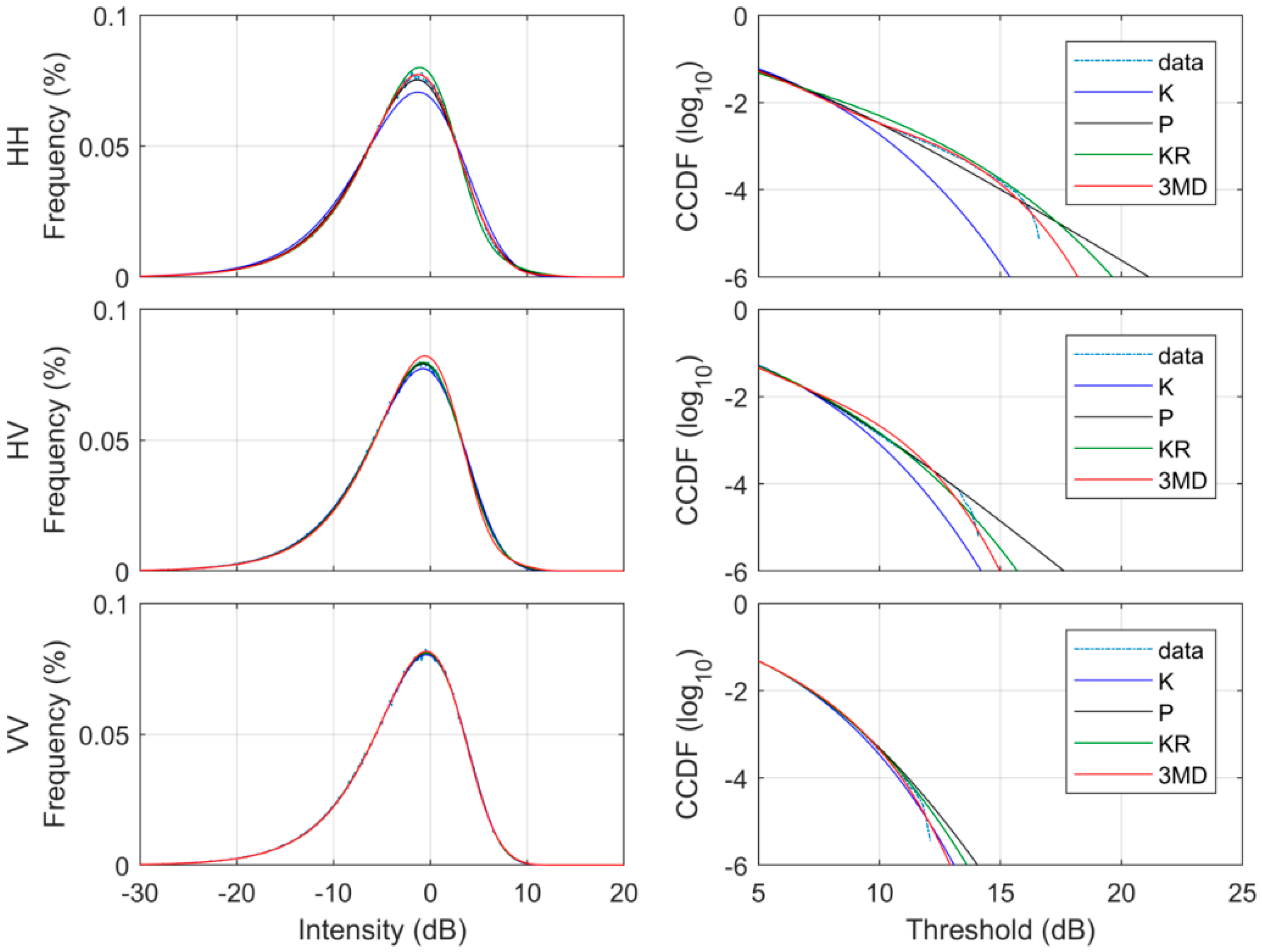
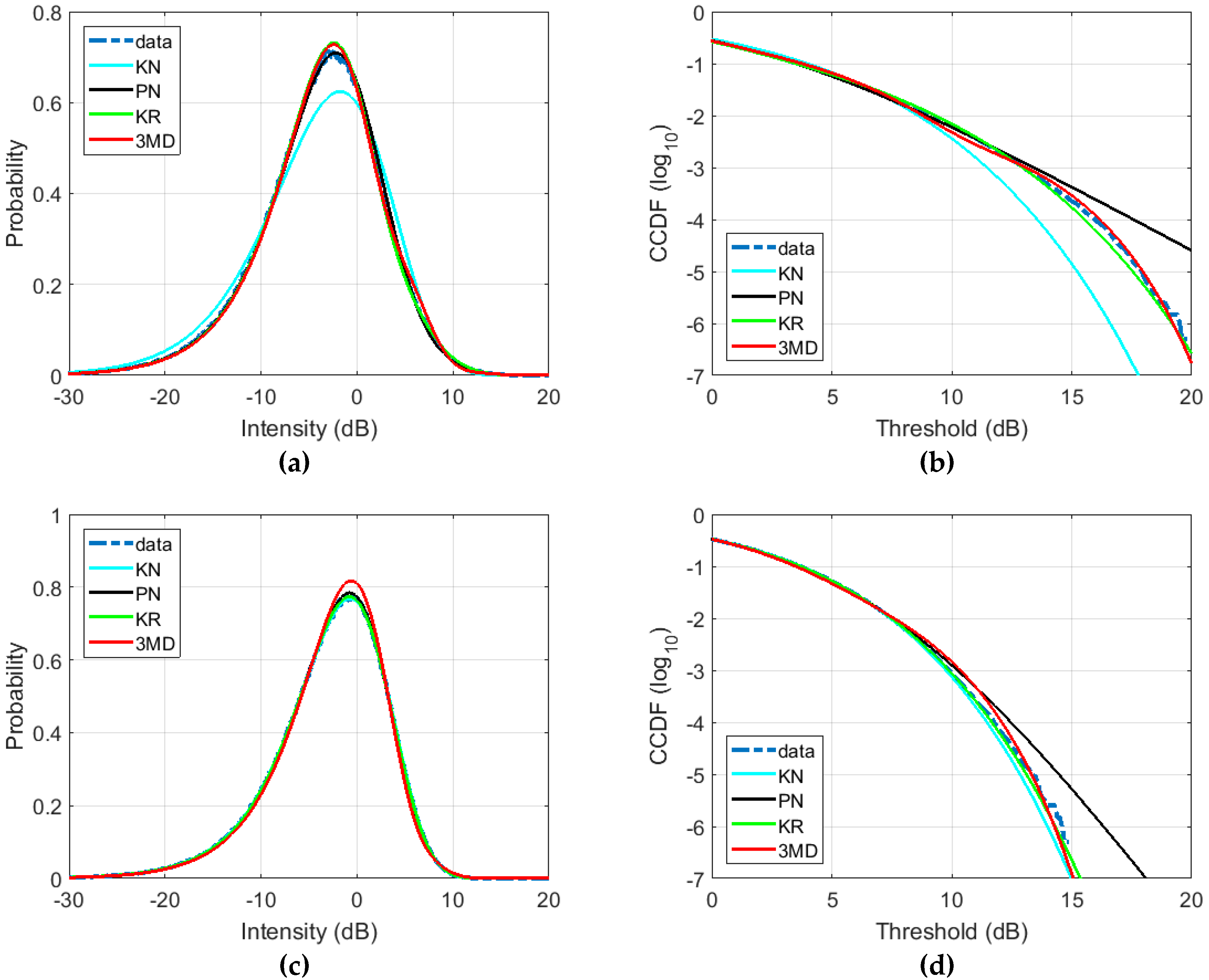
Examples of the model fits are shown in Figure 18 from Run 1 (see Table 3) at a grazing angle of 10° and a high sea state (wind speed of 17 m/s). For the HH polarization, the KN distribution deviates from the data PDF, while the PN, KR, and 3MD models show close agreeement to the real data (Figure 18a). In the tail of the distribution (Figure 18b), the KR and 3MD models show a good match the data, while the KN and PN both show mismatch. For the VV polarization (Figure 18c–d), we observe an overall good agreement between the data and the models, except for the PN distribution which over estimates the distribution tail (Figure 18d).

Table 9. Parameter estimates for the models in Figure 18.

Run 3	Polarization
	HH	VV
CNR (dB)	12.08	16.70
KN shape	1.45	5.56
PN shape	2.44	6.56
K+Rayleigh shape	0.19	2.69
K+Rayleigh $k_r$—value	0.47	0.27
3MD mode 1 (a, c)	(0.68, 0.65)	(0.88, 0.795)
3MD mode 2 (a, c)	(1.29, 0.33)	(1.39, 0.205)
3MD mode 3 (a, c)	(2.92, 0.02)	-

and

Table 10. Goodness of fit metrics for the model fits in Figure 18. Threshold error is measured at a CCDF of 10⁻⁴.

	BD (dB)		Threshold Error (dB)
	HH	VV	HH	VV
KN	−24.5	−41.0	2.88	0.23
PN	−38.0	−39.4	−1.27	−0.68
KR	−33.5	−41.5	0.22	−0.02
3MD	−36.5	−36.1	0.15	−0.06

show the model parameters and goodness of fit metrics for these results.

5.3.1. Grazing and Azimuth Angle Variation

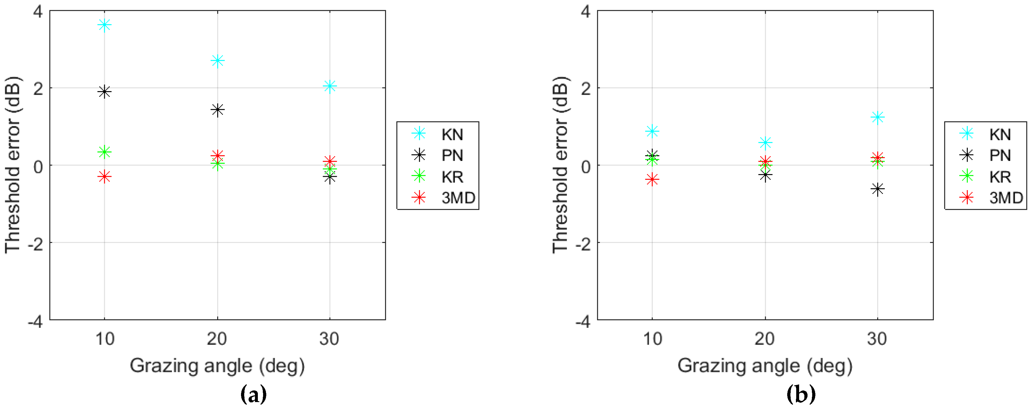
We now look at the goodness of fit for the SETHI data as a function of grazing and azimuth angles. The first set of results are for Runs 3 to 5 (see Table 3) with grazing angles of 10°, 20°, and 30° and a wind speed of 7 m/s.

Table 11. SETHI X-band Run 3 (grazing 10°), Run 4 (grazing 20°), and Run 5 (grazing 30°). Bhattacharyya distance (values in dB) between experimental and fitted PDFs.

Polarization	Grazing Angle	KN	PN	KR	3MD
HH	10°	−29.9	−36.4	−36.2	−38.4
	20°	−30.4	−34.5	−38.0	−39.0
	30°	−29.2	−35.9	−36.9	−37.6
VV	10°	−40.7	−49.9	−51.7	−35.2
	20°	−37.5	−39.4	−39.7	−38.1
	30°	−34.3	−37.5	−37.9	−38.4

shows the Bhattacharyya distance for the four models with good results (BD ≤ −30 dB) observed. Figure 19 then shows the threshold errors for CCDF values of 10⁻⁴. For the HH data, the threshold errors obtained with the KN and PN distributions decrease when the grazing angle increases, while KR and the 3MD distributions show a consistently low error. For the VV polarized radar data, the threshold errors are less than or equal to 1 dB for each model.

As with the INGARA results, there are no clear trends with the goodness of fit metrics as a function of wind direction. The next results consider the dual-frequency SAR data collected at 45° grazing and over the full 360° azimuth range (Run 8). For both the L and X-band datasets, histograms of the BD and threshold errors are shown in Figure 20 and Figure 21 at a CCDF value of 10⁻⁴. For the L-band data, the BD is low (≤−30 dB) for the four investigated models suggesting that they all match closely to the body of distribution, regardless of the polarization state. For the X-band data, the mean BD values increase for each model with the KN distribution showing the largest increase. There is also an increase in the spread of BD values at X-band. For the threshold error results, the 3MD distribution clearly has the lowest error at both frequencies with no bias around 0 dB. We find that the KN model has under fitted both data sets, while the PN and KR histograms show an over fitting. For the KN, PN, and KR models, the threshold error increases at X-band, probably due to data being spikier.

5.3.2. Wind Speed Variation

The final section looks at the fitting accuracy as the wind speed varies for the SETHI dataset. For this analysis, we consider three runs with grazing angles of 10° and 20° (see Table 3) and wind speeds of 7 m/s (Runs 3 and 4), 10 m/s (Runs 6 and 7) and 17 m/s (Runs 1 and 2). As with previous results, the BD is quite low, indicating a good fit to the distribution body. There is no observed trend or increase of the BD with the wind speed and the relative ordering of the four models are also similar to the previous results with the PN, KR, and 3MD distributions all having lower values than the KN model for the HH polarization, while all four models have similar BD values close to -40 dB for the VV polarization.

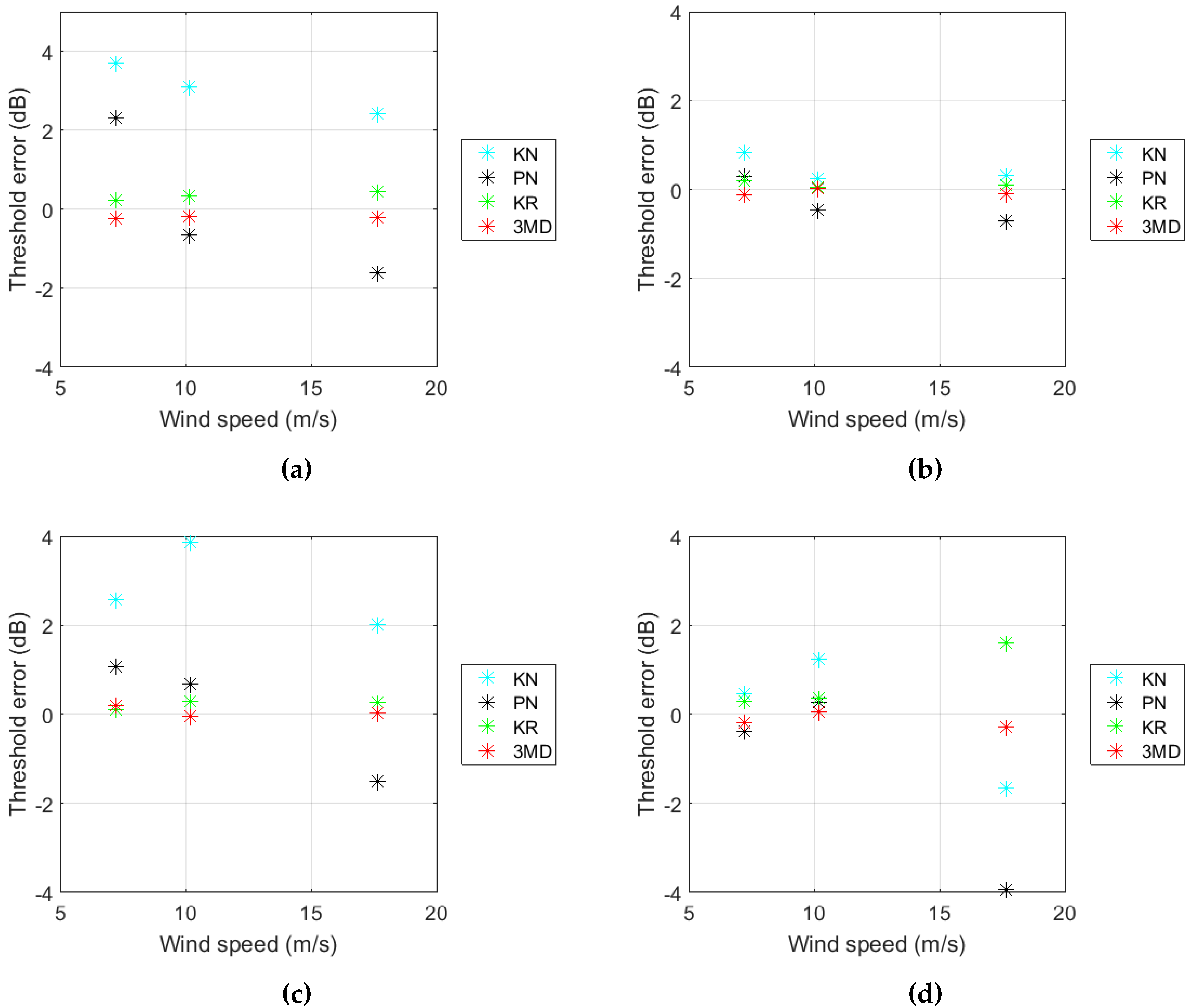
The threshold error for a CCDF of 10⁻⁴ is shown in Figure 22 for the HH and VV polarizations and both grazing angles. These results show quite similar errors for the KR and 3MD distributions with values typically below ±0.5 dB. There is one exception for the VV polarization with the higher wind speed and 20° grazing, where the KR model has overfitted the data. In this case, the 3MD model still produces a good fit with a low threshold error. No significant variation of the threshold error with the wind speed is observed.

5.3.3. Summary

Analysis of SETHI airborne SAR dataset presented in this section shows that the BD is always very low for the four investigated models, indicating that they can all accurately model the distribution body of the data. However, when we focus on the tail of the distribution, both the KR and 3MD distributions produce superior fits to the experimental data, especially for the HH polarization. Moreover, no significant variation of the threshold error with the wind speed and the angles of observation (grazing and azimuth) can be inferred from these results.

6. Conclusions

Accurately modeling the amplitude distribution of sea clutter is key to ensure good detection performance in the maritime domain. This can be a challenging task due to the wide variety of environmental conditions, collection geometries, and radar configurations. In this paper, we have evaluated the accuracy of four key amplitude distributions, the K+Noise, P+Noise, K+Rayleigh, and 3MD, in matching experimental high spatial resolution data from three different radar sensors. These include a ground-based radar collecting S-band mono- and bi-static data at very low grazing angles, an airborne sensor acquiring X-band full-polarized real aperture data and a second airborne fully-polarized SAR operating simultaneously at L- and X-band. The model accuracy was assessed using two goodness of fit measures: the Bhattacharyya distance which considered the body of the distribution, and the threshold error which focused on the tail.

The originality of the analysis is a quantitative evaluation of PDF models to represent actual radar sea clutter. This extends an earlier study [11] by expanding the range of frequency bands, collection geometries and amplitude distribution models. In

Table 12. Mean values of the Bhattacharyya distance for each dataset investigated in this study.

Dataset	Polarization	Bhattacharyya Distance (Mean Value—dB)
		KN	PN	KR	3MD
NetRAD	HH	−15.4	−23.7	−30.1	−37.5
	VV	−21.5	−23.5	−26.2	−35.2
INGARA	HH	−32.0	−34.1	−34.3	−32.8
	VV	−35.5	−35.3	−35.6	−35.4
SETHI	HH	−28.5	−37.7	−37.8	−33.2
	VV	−38.1	−40.2	−40.5	−35.2

and

Table 13. Mean values of the threshold error at a CCDF of 10⁻⁴ for each dataset investigated in this study.

Dataset	Polarization	Threshold Error (Mean Value—dB)
		KN	PN	KR	3MD
NetRAD	HH	4.7	−2.4	−0.2	0.2
	VV	2.7	−3.3	0.2	0.1
INGARA	HH	1.4	−0.8	0.0004	0.1
	VV	0.03	−0.3	−0.1	0.05
SETHI	HH	2.7	0.7	0.3	0.1
	VV	0.3	−1.3	0.4	0.1

below, a summary of the average Bhattacharyya distance and the threshold error measured at a CCDF of 10⁻⁴ is illustrated for each dataset. They demonstrate that both the KR and 3MD models provide a good match to the datasets studied, while the KN and PN distributions often show a mismatch. When focusing on the tail of the distribution, only the 3MD model consistently matches well, while the KR model has a slightly higher threshold error. The tradeoff with using the 3MD model is the larger number of parameters which require estimating.

Since the reported data covered such a wide range of frequencies, collection geometries, and sea conditions, these conclusions give confidence that these models would be applicable over a much wider range of conditions and with different radar sensors. In future work, we will focus on the improving the usefulness of the 3MD model. This can be achieved by speeding up the parameter estimation and understanding how the model parameters can be related to our understanding of the ocean scattering.

References

- Crisp, D.J. The State-of-the-Art in Ship Detection in Synthetic Aperture Radar Imagery; Research Report DSTO-RR-0272; Defence Science and Technology Organisation Australia: Fairbairn, Canberra, Australia, May 2004.
- Rosenberg, L. Sea-spike detection in high grazing angle X-band sea clutter. IEEE Trans. Geosci. Remote Sens. 2013, 51, 4556–4562. [Google Scholar] [CrossRef]
- Ward, K.D.; Tough, R.J.A.; Watts, S. Sea Clutter: Scattering, the K-Distribution and Radar Performance, 2nd ed.; The Institute of Engineering Technology UK: London, UK, 2013. [Google Scholar]
- Posner, F.L. Spiky sea clutter at high range resolutions and very low grazing angles. IEEE Trans. Aerosp. Electron. Syst. 2002, 38, 5872. [Google Scholar] [CrossRef]
- Fingas, M.F.; Brown, C.E. Review of ship detection from airborne platforms. Can. J. Remote Sens. 2001, 27, 379–385. [Google Scholar] [CrossRef]
- Angelliaume, S.; Ceamanos, X.; Viallefont-Robinet, F.; Baqué, R.; Déliot, P.; Miegebielle, V. Hyperspectral and Radar Airborne Imagery over Controlled Release of Oil at Sea. Sensors 2017, 17, 1772. [Google Scholar] [CrossRef] [PubMed]
- Jakeman, E.; Pusey, P. A model for non-Rayleigh sea echo. IEEE Trans. Antennas Propag. 1976, 24, 806–814. [Google Scholar] [CrossRef]
- Trunk, G.V.; George, S.F. Detection of targets in non-Gaussian sea clutter. IEEE Trans. Aerosp. Electron. Syst. 1970, 5, 620–628. [Google Scholar] [CrossRef]
- Schleher, D.C. Radar detection in Weibull Clutter. IEEE Trans. Aerosp. Electron. Syst. 1976, 12, 736–743. [Google Scholar] [CrossRef]
- Dong, Y. Distribution of X-Band High Resolution and High Grazing Angle Sea Clutter; Research Report, DSTO-RR-0316; Defence Science and Technology Organisation Australia: Fairbairn, Canberra, Australia, 2006.
- Fiche, A.; Angelliaume, S.; Rosenberg, L.; Khenchaf, A. Analysis of X-Band SAR Sea-Clutter Distributions at Different Grazing Angles. IEEE Trans. Geosci. Remote Sens. 2015, 53, 4650–4660. [Google Scholar] [CrossRef]
- Balleri, A.; Nehorai, A.; Wang, J. Maximum likelihood estimation for compound-Gaussian clutter with inverse gamma texture. IEEE Trans. Aerosp. Electron. Syst. 2007, 43, 775–779. [Google Scholar] [CrossRef]
- Weinberg, G.V. Assessing Pareto fit to high-resolution high-grazing angle sea clutter. IET Electron. Lett. 2011, 47, 516–517. [Google Scholar] [CrossRef]
- Rosenberg, L.; Bocquet, S. Application of the Pareto plus noise distribution to medium grazing angle sea-clutter. IEEE J. Sel. Top. Appl. Earth Obs. Remote Sens. 2015, 8, 255–261. [Google Scholar] [CrossRef]
- Lamont-Smith, T. Translation to the normal distribution for radar clutter. IEE Proc. Radar Sonar Navig. 2000, 147, 17–22. [Google Scholar] [CrossRef]
- Rosenberg, L.; Watts, S.; Bocquet, S. Application of the K+Rayleigh distribution to high grazing angle sea-clutter. In Proceedings of the International Radar Conference, Lille, France, 13–17 October 2014; pp. 1–6. [Google Scholar]
- Gierull, C.H.; Sikaneta, I. A Compound-Plus-Noise Model for Improved Vessel Detection in Non-Gaussian SAR Imagery. IEEE Trans. Geosci. Remote Sens. 2018, 56, 1444–1453. [Google Scholar] [CrossRef]
- Kil, D.H.; Shin, F.B. Pattern Recognition and Prediction with Applications to Signal Processing; Springer: New York, NY, USA, 1998. [Google Scholar]
- Rosenberg, L.; Bocquet, S. Non-coherent radar detection performance in medium grazing angle X-band sea-clutter. IEEE Trans. Aerosp. Electron. Sens. 2017, 53, 669–682. [Google Scholar] [CrossRef]
- Bocquet, S. Parameter estimation for Pareto and K distributed clutter with noise. IET Radar Sonar Navig. 2015, 9. [Google Scholar] [CrossRef]
- Ward, K.D. Compound representation of high resolution sea clutter. Electron. Lett. 1981, 17, 561–563. [Google Scholar] [CrossRef]
- Derham, T.; Doughty, S.; Woodbridge, K.; Baker, C. Design and evaluation of a low-cost multistatic netted radar system. IET Radar Sonar Navig. 2007, 1, 362–368. [Google Scholar] [CrossRef]
- Ritchie, M.; Stove, A.; Woodbridge, K.; Griffiths, H. NetRAD: Monostatic and Bistatic Sea Clutter Texture and Doppler Spectra Characterization at S-Band. IEEE Trans. Geosci. Remote Sens. 2016, 54, 5533–5543. [Google Scholar] [CrossRef]
- Rosenberg, L.; Watts, S. High Grazing Angle Sea-Clutter Literature Review; General Document; DSTO-GD-0736; Defence Science and Technology Organisation Australia: Fairbairn, Canberra, Australia, March 2013.
- Valenzuela, G.R. Theories for the interaction of electromagnetic and oceanic waves—A review. Bound. -Layer Meteorol. 1978, 13, 61–82. [Google Scholar] [CrossRef]
- Rosenberg, L.; Angelliaume, S. Characterisation of the Tri-Modal Discrete Sea Clutter Model. In Proceedings of the International Radar Conference, Brisbane, Australia, 27–30 August 2018; pp. 1–6. [Google Scholar]
Figure 1.
Illustration of an X-band SAR image in the Mediterranean Sea—blue box: target free area, red box: sea surface including a ship.
Figure 2.
CCDF computed over the two areas shown in Figure 1—blue box: target free area, red box: sea surface including a ship.
Figure 3.
Measurement of the threshold error at 10−4 between the actual CCDF (blue thick dotted line) and the model CCDF (green line).
Figure 4.
NetRAD: S-band time domain intensity images, monostatic (left), and bistatic 60° (right) for HH (top) and VV (bottom) polarizations.
Figure 5.
INGARA range/time example (Run 3), downwind, grazing angle 30°, wind speed 10.3 m/s.
Figure 6.
SETHI X-band SAR images (Run 3), grazing angle 10°, wind speed 7 m/s. (a) HH polarization, (b) VV polarization.
Figure 7.
Amplitude distributions for the NetRAD data (Run 4): S-band, HH-polarization, bistatic acquisition, bistatic angle 60°. Illustrations show the (a) PDF, (b) CCDF.
Figure 8.
Model fits for the 3MD distribution with different numbers of modes using the NetRAD data S-band, VV-polarization, bistatic configuration, 60° bistatic angle (Run 1). Illustrations show the (a) PDF, (b) CCDF.
Figure 9.
Bhattacharyya distance (dB scale) for the 3MD distribution using different numbers of modes with the NetRAD data, S-band, bistatic configuration, 60° bistatic angle. (a) HH polarization (Run 4), (b) VV polarization (Run 1).
Figure 10.
NetRAD S-band: Bhattacharyya distance (in dBs) for the NetRAD data. (a) HH polarization, monostatic, (b) HH polarization, bistatic, (c) VV polarization, monostatic, (d) VV polarization, bistatic.
Figure 11.
NetRAD S-band: Threshold error for a CCDF of 10−4. (a) HH polarization, monostatic, (b) HH polarization, bistatic, (c) VV polarization, monostatic, (d) VV polarization, bistatic.
Figure 12.
Amplitude distributions for the INGARA dataset (Run 3), upwind, grazing angle 30°. Illustrations show the (left) PDF and (right) CCDF results.
Figure 13.
3MD distribution parameters () for the INGARA dataset, Run 3.
Figure 14.
3MD distribution parameters () for the INGARA dataset, Run 9.
Figure 15.
BD histograms for INGARA Runs 3 and 9. (a) Run 3, (b) Run 9.
Figure 16.
Threshold error histograms for INGARA Runs 3 and 9. Threshold error is measured at a CCDF of 10−4. (a) Run 3, (b) Run 9.
Figure 17.
Threshold error against windspeed in the upwind direction for the INGARA dataset. Threshold error is measured at a CCDF of 10−4.
Figure 18.
Amplitude distributions of the SETHI dataset, (Run 1), grazing angle 10°, wind speed 17 m/s. (a) HH polarization PDF, (b) HH polarization CCDF, (c) VV polarization PDF, (d) VV polarization CCDF.
Figure 19.
Threshold error with increasing grazing angle for SETHI X-band Runs 3 to 5 (wind speed 7 m/s). Threshold error is measured at a CCDF of 10−4. (a) HH, (b) VV.
Figure 20.
BD histogram for SETHI, Run 8. (a) X-band, (b) L-band.
Figure 21.
Threshold error histogram for SETHI, Run 8. Threshold error is measured at a CCDF of 10−4. (a) X-band, (b) L-band.
Figure 22.
Threshold error against windspeed for the SETHI X-band dataset. Threshold error is measured at a CCDF of 10−4. (a) HH polarization, 10° grazing; (b) VV polarization, 10° grazing; (c) HH polarization, 20° grazing; (d) VV polarization, 20° grazing.