Remote Sensing Image Scene Classification Using CNN-CapsNet


1
National Engineering Laboratory for Applied Technology of Remote Sensing Satellites, Institute of Remote Sensing and Digital Earth of Chinese Academy of Sciences, Beijing 100101, China
2
University of Chinese Academy of Sciences, Beijing 100049, China
*
Author to whom correspondence should be addressed.
Remote Sens. 2019, 11(5), 494; https://doi.org/10.3390/rs11050494
Submission received: 7 January 2019
/
Revised: 20 February 2019
/
Accepted: 22 February 2019
/
Published: 28 February 2019
(This article belongs to the Special Issue Very High Resolution (VHR) Satellite Imagery: Processing and Applications)
Abstract
:Remote sensing image scene classification is one of the most challenging problems in understanding high-resolution remote sensing images. Deep learning techniques, especially the convolutional neural network (CNN), have improved the performance of remote sensing image scene classification due to the powerful perspective of feature learning and reasoning. However, several fully connected layers are always added to the end of CNN models, which is not efficient in capturing the hierarchical structure of the entities in the images and does not fully consider the spatial information that is important to classification. Fortunately, capsule network (CapsNet), which is a novel network architecture that uses a group of neurons as a capsule or vector to replace the neuron in the traditional neural network and can encode the properties and spatial information of features in an image to achieve equivariance, has become an active area in the classification field in the past two years. Motivated by this idea, this paper proposes an effective remote sensing image scene classification architecture named CNN-CapsNet to make full use of the merits of these two models: CNN and CapsNet. First, a CNN without fully connected layers is used as an initial feature maps extractor. In detail, a pretrained deep CNN model that was fully trained on the ImageNet dataset is selected as a feature extractor in this paper. Then, the initial feature maps are fed into a newly designed CapsNet to obtain the final classification result. The proposed architecture is extensively evaluated on three public challenging benchmark remote sensing image datasets: the UC Merced Land-Use dataset with 21 scene categories, AID dataset with 30 scene categories, and the NWPU-RESISC45 dataset with 45 challenging scene categories. The experimental results demonstrate that the proposed method can lead to a competitive classification performance compared with the state-of-the-art methods.
1. Introduction
With the development of Earth observation technology, many different types (e.g., multi/hyperspectral [1] and synthetic aperture radar [2]) of high-resolution images of the Earth’s surface are readily available. Therefore, it is particularly important to effectively understand their semantic content, and more intelligent identification and classification methods of land use and land cover (LULC) are definitely demanded. Remote sensing image scene classification, which aims to automatically assign a specific semantic label to each remote sensing image scene patch according to its contents, has become an active research topic in the field of remote sensing image interpretation because of its vital applications in LULC, urban planning, land resource management, disaster monitoring, and traffic control [3,4,5,6].
During the last decades, several methods have been developed for remote sensing image scene classification. The early methods for scene classification were mainly based on low-level features or hand-crafted features, which focus on designing various human-engineering features locally or globally, such as color, texture, shape, and spatial information. Representative features, including the scale invariant feature transform (SIFT), color histogram (CH), local binary pattern (LBP), Gabor filters, grey level cooccurrence matrix (GLCM), and the histogram of oriented gradients (HOG) or their combinations, are usually used for scene classification [7,8,9,10,11,12]. It is worth noting that methods relying on these low-level features perform well on some images with uniform texture or spatial arrangements, but they are still limited for distinguishing images with more challenging and complex scenes, which is because the involvement of humans in feature design significantly influences the effectiveness of the representation capacity of scene images. In contrast to low-level feature-based methods, the mid-level feature approaches attempt to compute a holistic image representation formed by local visual features such as SIFT, color histogram, or LBP of local image patches. The general pipeline of building mid-level features is to extract local attributes of image patches first and then to encode them to obtain the mid-level representation of remote sensing images. The well-known bag-of-visual-words (BoVW) model is the most popular mid-level approach and has been widely adopted for remote sensing image scene classification because of its simplicity and effectiveness [13,14,15,16,17,18]. The methods based on the BoVW have improved the classification performance, but due to the limitation of representation capability of the BOVW model, no further breakthroughs have been achieved for remote sensing image scene classification.
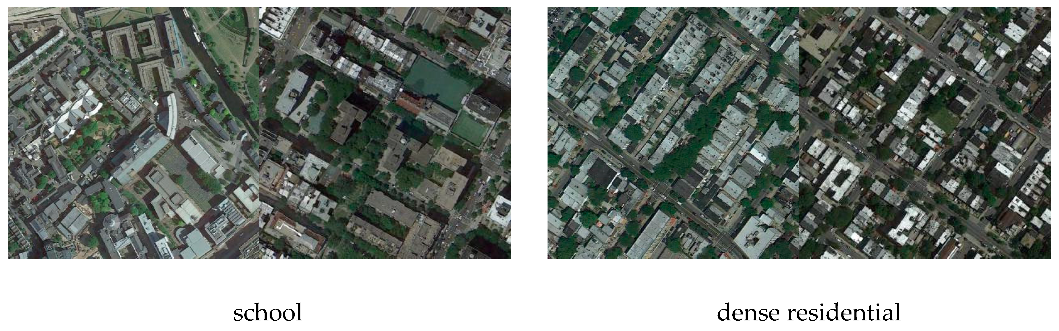
Recently, with the prevalence of deep learning methods, which have achieved impressive performance on many applications including image classification [19], object recognition [20], and semantic segmentation [21], the feature representation of images has stepped into a new era. Unlike low-level and mid-level features, deep learning models can learn more powerful, abstract and discriminative features via deep-architecture neural networks without a considerable amount of engineering skill and domain expertise. All of these deep learning models, especially the convolutional neural network (CNN), are more applicable for remote sensing image scene classification and have achieved state-of-the-art results [22,23,24,25,26,27,28,29,30,31,32,33,34]. Although the CNN-based methods have dramatically improved classification accuracy, some scene classes are still easily mis-classified. Taking the AID dataset as an example, the class-specific classification accuracy of ‘school’ is only 49% [35], which is usually confused with ‘dense residential’. As shown in Figure 1, two images labelled ‘school’ and two images labelled ‘dense residential’ have been selected from the AID dataset. We can see that the contexts among these four images have similar image distribution and all contain many buildings and trees. However, different from the arrangement irregularity of buildings in ‘school’, the buildings in ‘dense residential’ are arranged closely and orderly. This spatial layout difference between them is very helpful in distinguishing the two classes and should be given more consideration in the phase of classification. However, the use of the fully connected layer at the end of the CNN model compresses the two-dimensional feature map into a one-dimensional feature map and cannot fully consider the spatial relationship, which makes it difficult to distinguish the two classes.
Recently, the advent of the capsule network (CapsNet) [36], which is a novel architecture to encode the properties and spatial relationship of the features in an image and is a more effective image recognition algorithm, shows encouraging results on image classification. Although the CapsNet is still in its infancy [37], it has been successfully applied in many fields [38,39,40,41,42,43,44,45,46,47,48,49] in recent years, such as brain tumor classification, sound event detection, object segmentation, and hyperspectral image classification. The CapsNet uses a group of neurons as a capsule to replace a neuron in the traditional neural network. In addition, the capsule is a vector to represent internal properties that can be used to learn part–whole relationships between various entities, such as objects or object parts, to achieve equivariance [36] and can solve the problem of traditional neural networks using fully connected layers cannot efficiently capture the hierarchical structure of the entities in images to preserve the spatial information [50].
To further improve the accuracy of the remote sensing image scene classification and motivated by the powerful ability of feature learning of deep CNN and the property of equivariance of CapsNet, a new architecture named CNN-CapsNet is proposed to deal with the task of remote sensing image scene classification in this paper. The proposed architecture is composed of two parts. First, a pretrained deep CNN, such as VGG-16 [51], is fully trained on the ImageNet [52] dataset, and its intermediate convolutional layer is used as an initial feature maps extractor. Then, the initial feature maps are fed into a newly designed CapsNet to label the remote sensing image scenes. Experimental results on three challenging benchmark datasets show that the proposed architecture achieves a more competitive accuracy compared with state-of-the-art methods. In summary, the major contributions of this paper are as follows:
- To further improve classification accuracy, especially classes that have high homogeneity in the image content, a new novel architecture named CNN-CapsNet is proposed to deal with the remote sensing image scene classification problem, which can discriminate scene classes effectively.
- By combining the CNN and the CapsNet, the proposed method can obtain a superior result compared with the state-of-the-art methods on three challenging datasets without any data-augmentation operation.
- This paper also analyzes the influence of different factors in the proposed architecture on the classification result, including the routing number in the training phase, the dimension of capsules in the CapsNet and different pretrained CNN models, which can provide valuable guidance for subsequent research on the remote sensing image scene classification using CapsNet.
The remainder of this paper is organized as follows. In Section 2, the materials are illustrated. Section 3 introduces the theory of CNN and CapsNet first, and then describes the proposed method in detail. Section 4 analyzes the influence of different factors, and discusses the experimental results of the proposed method. Finally, conclusions are drawn in Section 5.
2. Materials
Three popular remote sensing datasets (UC Merced Land-Use [14], AID [35], and NWPU-RESISC45 [53]) with different visual properties are chosen to better demonstrate the robustness and effectiveness of the proposed method. In addition, details about the datasets are described in Section 2.1, Section 2.2 and Section 2.3.
2.1. UC Merced Land-Use Dataset
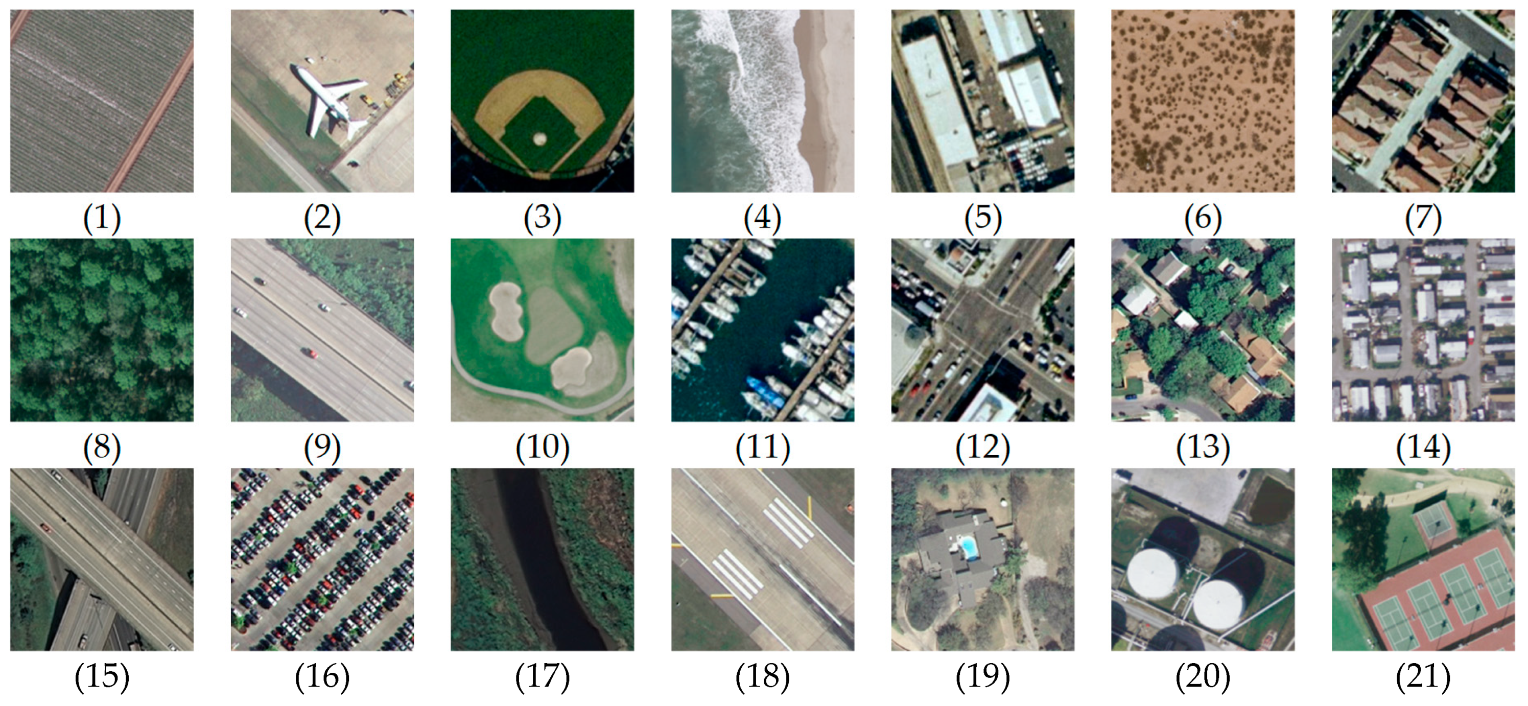
The UC Merced Land-Use dataset is composed of 2100 aerial scene images divided into 21 land use scene classes, as shown in Figure 2. Each class contains 100 images with size of 256 × 256 pixels with a pixel spatial resolution of 0.3 m in the red green blue (RGB) color space. These images were selected from aerial orthoimagery downloaded from the United States Geological Survey (USGS) National Map of the following US regions: Birmingham, Boston, Buffalo, Columbus, Dallas, Harrisburg, Houston, Jacksonville, Las Vegas, Los Angeles, Miami, Napa, New York, Reno, San Diego, Santa Barbara, Seattle, Tampa, Tucson, and Ventura. It is not only the diversity of land-use categories contained in the dataset that makes it challenging. Some highly overlapped classes such as dense residential, medium residential and sparse residential are included in this dataset, which are mainly different in the density of structures and makes the dataset more difficult to classify. This dataset has been widely used for the task of remote sensing image scene classification [18,23,24,25,27,28,30,32,54,55,56,57,58].
2.2. AID Dataset
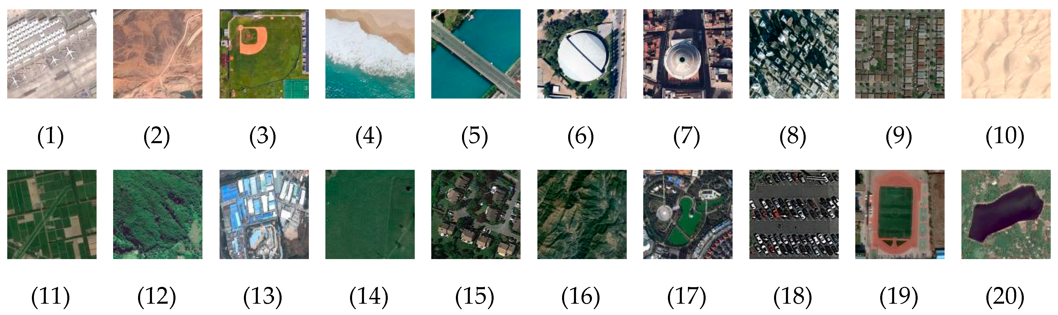
AID is large-scale aerial image dataset, which was collected from Google Earth imagery and is a more challenging dataset compared with the UC Merced Land-Use dataset because of the following reasons. First, the AID dataset contains more scene types and images. In detail, it has 10,000 images with a fixed size of 600 × 600 pixels within 30 classes as shown in Figure 3. Some similar classes make the interclass dissimilarity smaller, and the number of images of different scene types differs from 220 to 420. Moreover, AID images were chosen under different times and seasons and different imaging conditions, and from different countries and regions around the world, including China, the United States, England, France, Italy, Japan, and Germany, which definitely increases the intraclass diversities. Finally, AID images have the property of multiresolution, changing from approximately 8 m to about half a meter.
2.3. NWPU-RESISC45 Dataset
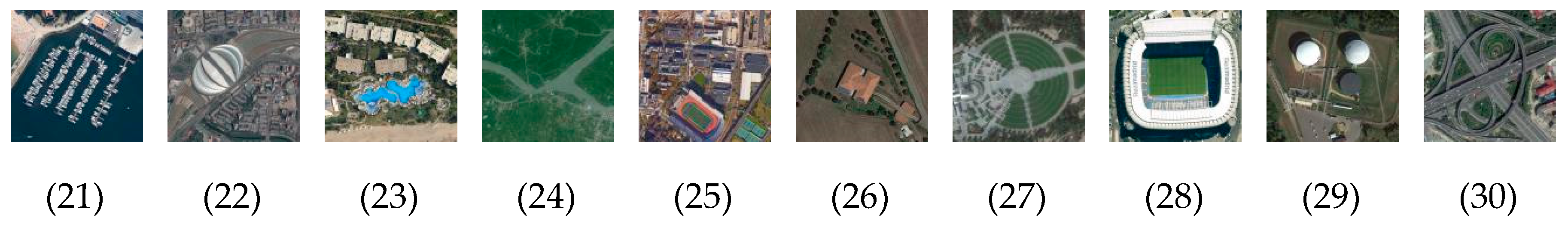
NWPU-RESISC45 dataset is more complex than UC Merced Land-Use and AID datasets and consists of a total of 31,500 remote sensing images divided into 45 scene classes as shown in Figure 4. Each class includes 700 images with a size of 256 × 256 pixels in the RGB color space. This dataset was extracted from Google Earth by the experts in the field of remote sensing image interpretation. The spatial resolution varies from approximately 30 to 0.2 m per pixel. This dataset covers more than 100 countries and regions all over the world with developing, transitional, and highly developed economies.
3. Method
In this section, a brief introduction about CNN and CapsNet will be made first and then the proposed architecture will be detailed.
3.1. CNN
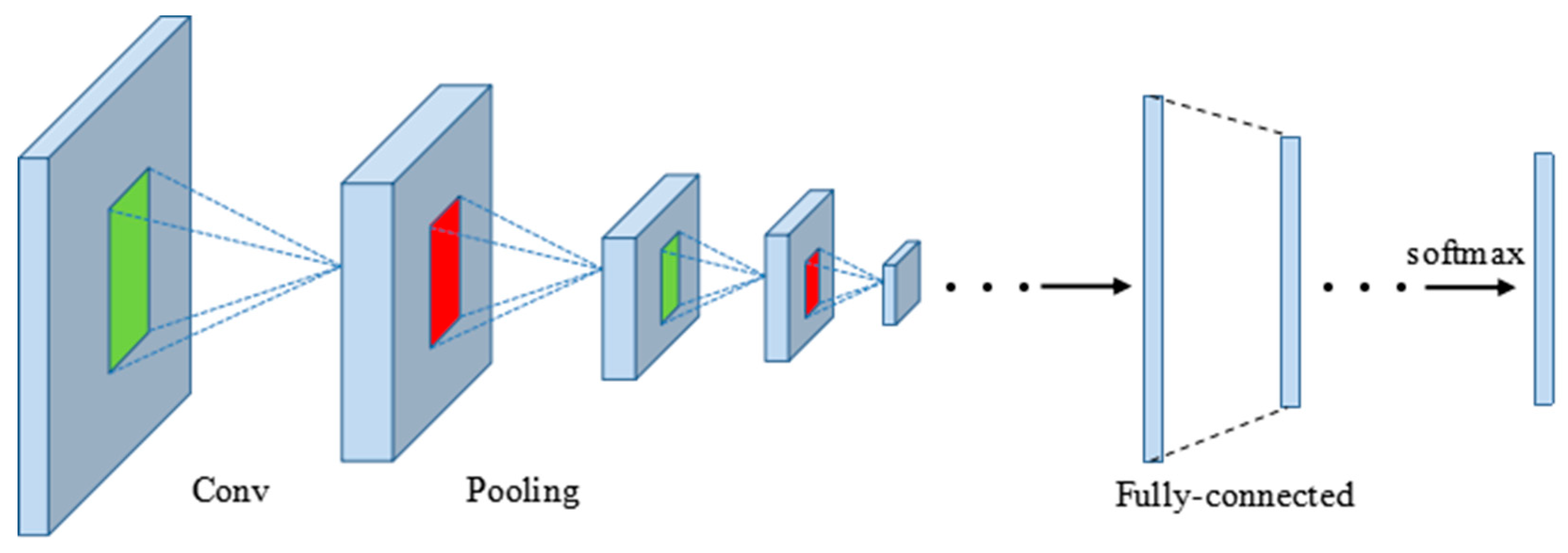
The convolutional neural network is a type of feed-forward artificial neural network, which is biologically inspired by the organization of the animal visual cortex. They have wide applications in image and video recognition, recommender systems and natural language processing. As shown in Figure 5, CNN is generally made up of two main parts: convolutional layers and pooling layers. The convolutional layer is the core building block of a CNN, which outputs feature maps by computing a dot product between the local region in the input feature maps and a filter. Each of the feature maps is followed by a nonlinear function for approximating arbitrarily complex functions and squashing the output of the neural network to be within certain bounds, such as the rectified linear unit (ReLU) nonlinearity, which is commonly used because of its computational efficiency. The pooling layer performs a downsampling operation to feature maps by computing the maximum or average value on a sub-region. Usually, the fully connected layers follow several stacked convolutional and pooling layers and the last fully connected layer is the softmax layer computing the scores for each class.
3.2. CapsNet
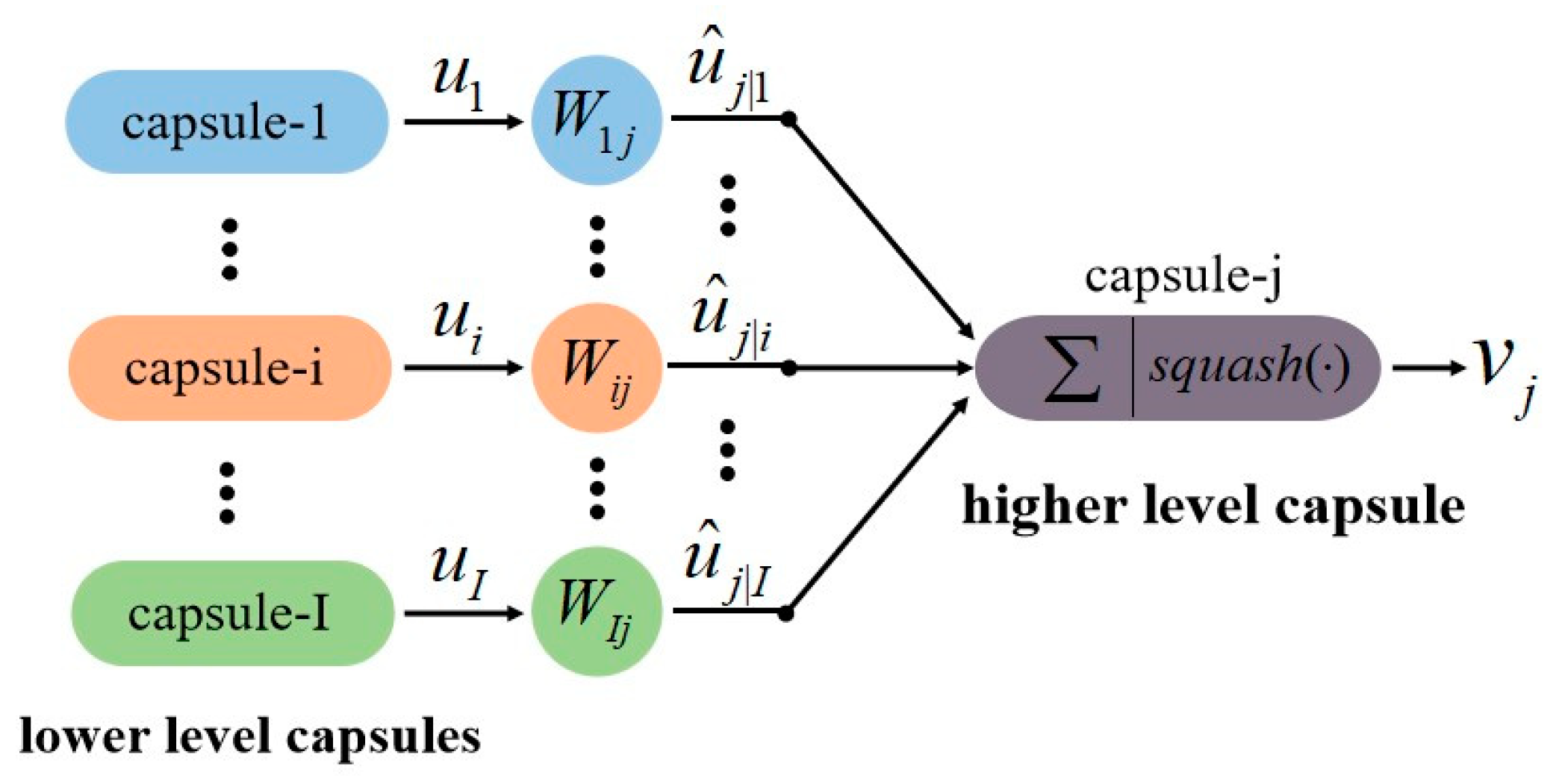
CapsNet is a completely novel deep learning architecture, which is robust to affine transformation [41]. In CapsNet, a capsule is defined as a vector that consists of a group of neurons, whose parameters can represent various properties of a specific type of entity that is presented in an image, such as position, size, and orientation. The length of each activity vector provides the existence probability of the specific object, and its orientation indicates its properties. Figure 6 illustrates the way that CapsNet routes the information from one layer to another layer by a dynamic routing mechanism [36], which means capsules in lower levels predict the outcome of capsules in higher levels and higher level capsules are activated only if these predictions agree.
Considering ui as the output of lower-level capsule i, its prediction for higher level capsule j is computed as:
where Wij is the weighting matrix that can be learned by back-propagation. Each capsule tries to predict the output of higher level capsules, and if this prediction conforms to the actual output of higher level capsules, the coupling coefficient between these two capsules increases. Based on the degree of conformation, coupling coefficients are calculated using the following softmax function:
where bij is set to 0 initially at the beginning of routing by an agreement process and is the log probability of whether lower-level capsule i should be coupled with higher level capsule j. Then, the input vector to the higher level capsule j can be calculated as follows:
Because the length of the output vector represents the probability of existence, the following nonlinear squash function, which is an activation function to ensure that short vectors are decreased to almost zero, and the long vectors are close to one, is used on the output vector computed in Equation (3) to prevent the output vectors of capsules from exceeding one.
where sj and vj represent the input vector and output vector, respectively, of capsule j. In addition, the log probabilities bij is updated in the routing process based on the agreement between vj and ûj|i according to the rule that if the two vectors agree, they will have a large inner product. Therefore, agreement aij for updating log probabilities bij and coupling coefficients cij is calculated as follows:
As mentioned above, Equations (2)–(5) make up one whole routing procedure for computing vj. The routing algorithm consists of several iterations of the routing procedure [36], and the number of iterations can be described as the routing number. Take the ‘school’ scene type detection as an example for a clearer explanation. Lengths of the outputs of the lower-level capsules (u1, u2, …, uI) encode the existence probability of their corresponding entities (e.g., building, tree, road, and playground). Directions of the vectors encode various properties of these entities, such as size, orientation, and position. In training, the network gradually encodes the corresponding part-whole relationship by a routing algorithm to obtain a higher-level capsule (vj), which encodes the whole scene contexts that the ‘school’ represents. Thus, the capsule can learn the spatial relationship between entities within an image.
Each capsule k in the last layer is associated with a loss function lk, which can be computed as follows:
where Tk is 1 when class k is actually present, m+, m− and λ are hyper-parameters that should be indicated while training. The total loss is simply the sum of the loss of all output capsules of the last layer.
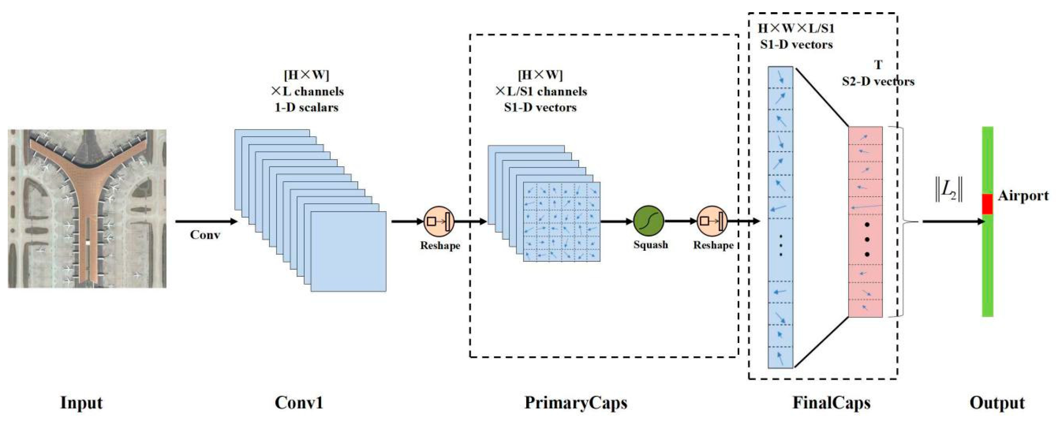
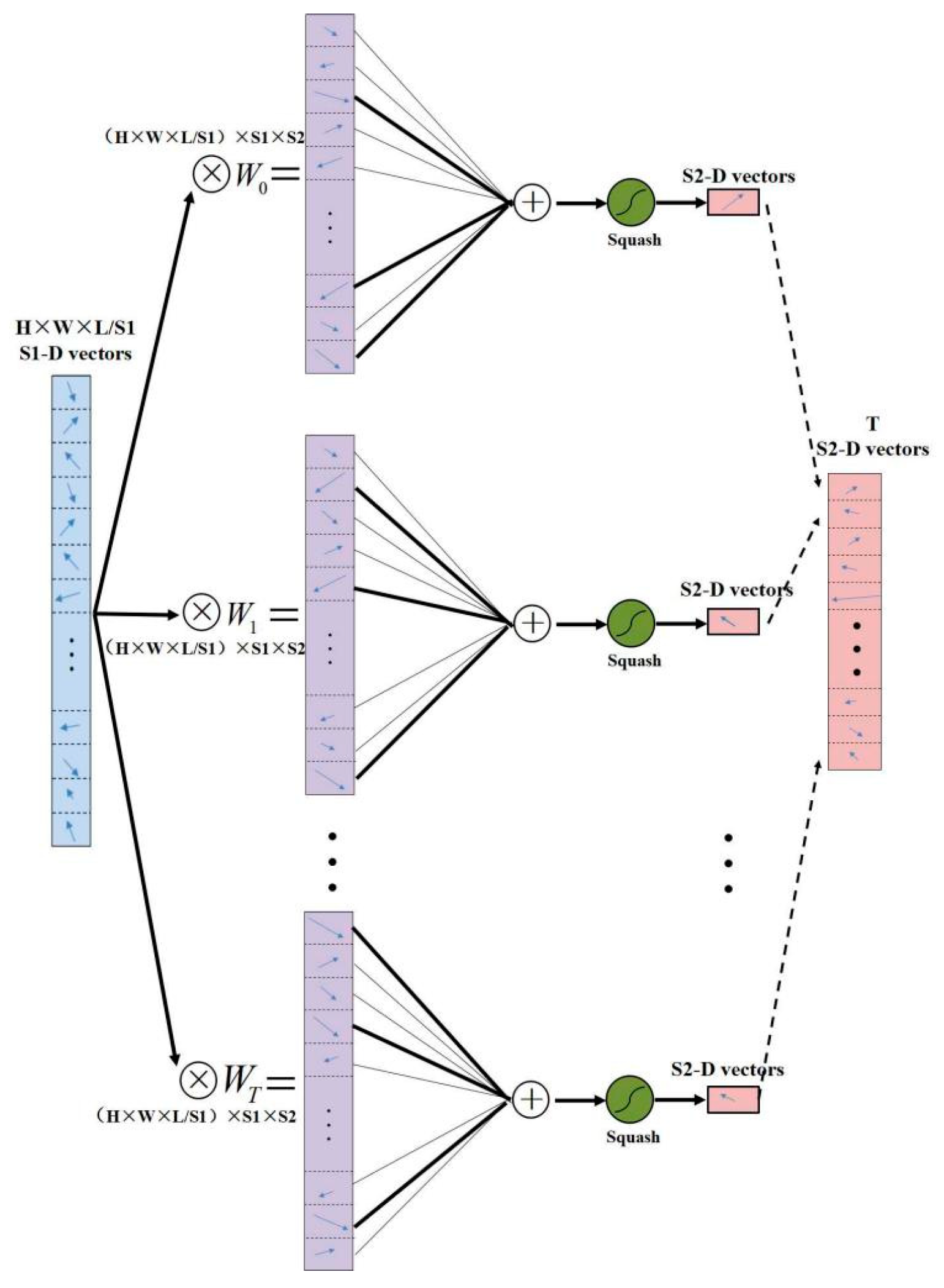
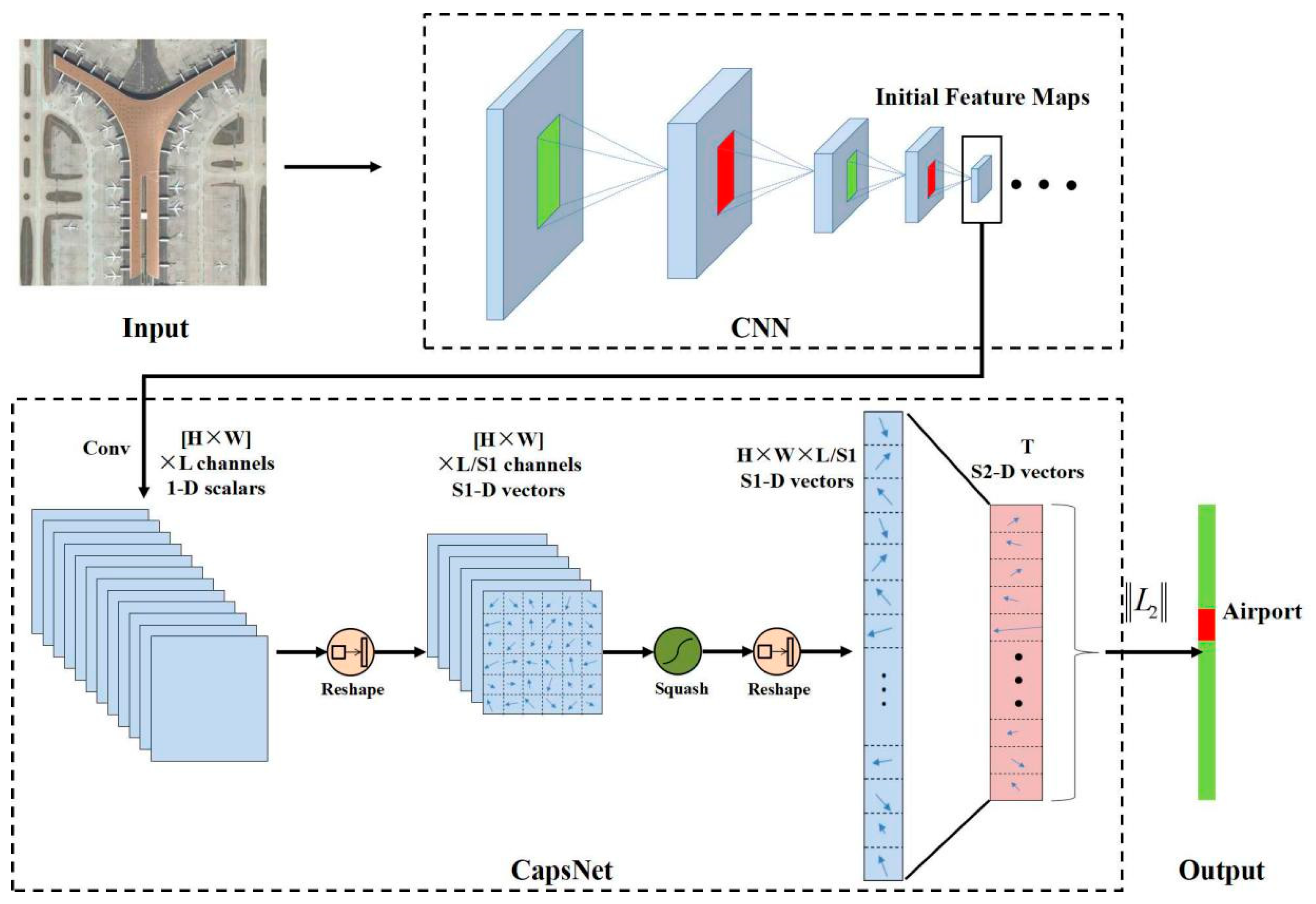
A typical CapsNet is shown in Figure 7 and contains three layers: one convolutional layer (Conv1), the PrimaryCaps layer and the FinalCaps layer. The Conv1 converts the input image (raw pixels) to initial feature maps, whose size can be described as H × W × L. Then, by two reshape functions and one squash operation, the PrimaryCaps can be computed, which contains H × W × L/S1 capsules (each capsule in the PrimaryCaps is an S1 dimension vector and is denoted as the S1-D vector in Figure 7). The FinalCaps has T (number of total predict classes) capsules (each capsule in the FinalCaps is an S2 dimension vector and is denoted as the S2-D vector in Figure 7), and each of these capsules receives input from all the capsules in the PrimaryCaps layer. The detail of FinalCaps is illustrated in Figure 8. At the end of the CapsNet, the length of each capsule in FinalCaps is computed by an L2 norm function, the corresponding scene category represented by the maximum value is the final classification result.
3.3. Proposed Method
As illustrated in Figure 9, the proposed architecture CNN-CapsNet can be divided into two parts: CNN and CapsNet. First, a remote sensing image is fed into a CNN model, and the initial feature maps are extracted from the convolutional layers. Then, the initial feature maps are fed into CapsNet to obtain the final classification result.
As for CNN, two representative CNN models (VGG-16 and Inception-V3) fully trained on the ImageNet dataset are used as initial feature map extractors, considering their popularity in the remote sensing field [25,27,28,35,53,56,59]. The “block4_pool” layer of VGG-16 and the “mixd7” of Inception-V3 are selected as the layer of initial feature maps, whose sizes are 16 × 16 × 512 and 14 × 14 × 768, respectively, if the input image size is 256 × 256 pixels. The influence of the two pretrained CNN models on the classification results is discussed in Section 4.2. In addition, a brief introduction about them follows.
- VGG-16: Simonyan et al. [51] presented the very deep CNN models that secured the first and the second places in the localization and classification tracks, respectively, on ILSVRC2014. The two best-performing deep models, named VGG-16 (containing 13 convolutional layers and 3 fully connected layers) and VGG-19 (containing 16 convolutional layers and 3 fully connected layers) are the basis of their team’s submission, which demonstrates the important aspect of the model’s depth. Rather than using relatively large receptive fields in the convolutional layers, such as 11 × 11 with stride 4 in the first convolutional layer of AlexNet [60], VGGNet uses very small 3 × 3 receptive fields through the whole network. VGG-16 is the most representative sequence-like CNN architecture as shown in Figure 5 (consisting of a simple chain of blocks such as the convolution layer and pooling layer), which has achieved great success in the field of remote sensing image scene classification.
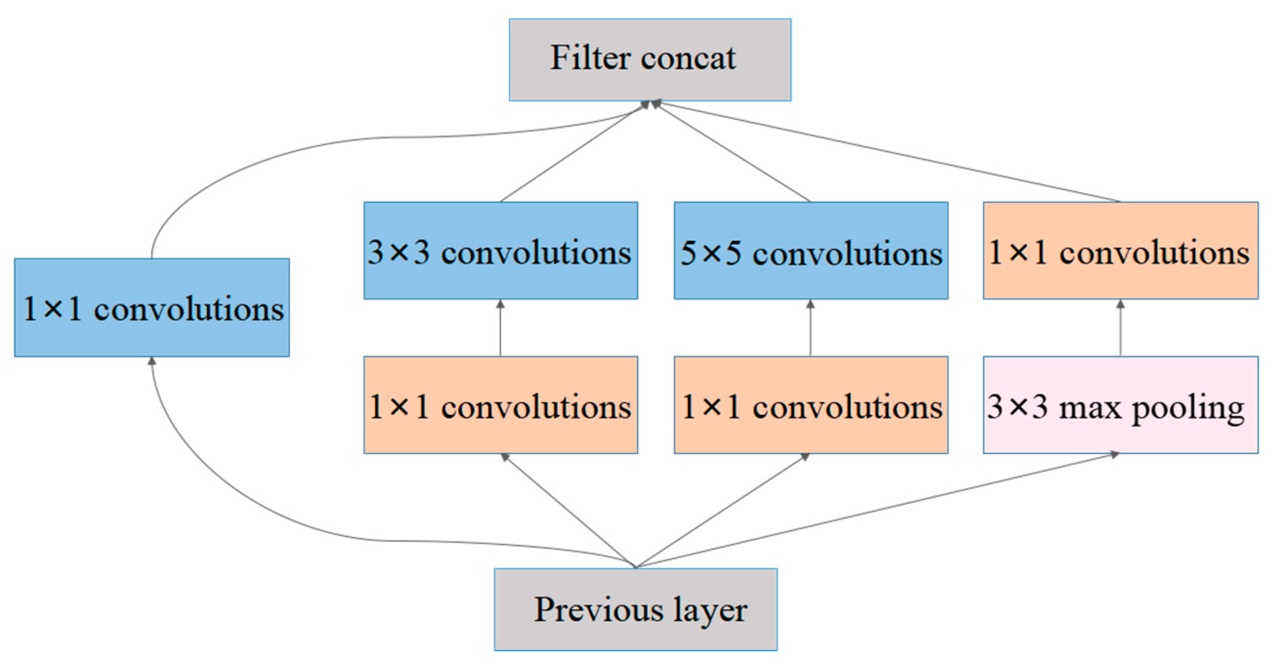
- Inception-v3: Unlike the sequence-like CNN architecture such as VGG-16, which only increases the depth of the convolution layers, the Inception-like CNN architecture attempts to increase the width of a single convolution layer, which means different sizes of kernels are used on the single convolution layer and can extract different scales of features. As shown in Figure 10, it is the core component of GoogLeNet [61] named Inception-v1. Inception-v3 [62] is an improved version of Inception-v1 and is designed on the following four principles: to avoid representation bottlenecks, especially early in the network; higher dimensional representations are easier to process locally within a network; spatial aggregation can be done over lower dimensional embedding without much or any loss in representation; to balance the width and depth of the network. The Inception-v3 reached 21.2% top-1 and 5.6% top-5 error on the ILSVR 2012 classification.
For CapsNet, a CapsNet with an analogical architecture as shown in Figure 7 is designed, including three layers: one convolutional layer, one PrimaryCaps layer and one FinalCaps layer. A 5 × 5 convolution kernel with a stride of 2, and a ReLU activation function is used in the convolution layer. The number of output feature maps (the variable L) is set as 512. The dimension of the capsules in the PrimaryCaps and FinalCaps layers (the variables S1 and S2) are the vital parameters of the CapsNet and their influence on the classification result is discussed in Section 4.2. The variable T is determined by the remote sensing datasets and is set as 21, 30, and 45 for the UC Merced Land-Use dataset, AID dataset and NWPU-RESISC45 dataset, respectively. In addition, 50% dropout was used between the PrimaryCaps layer and the FinalCaps layer to prevent overfitting.
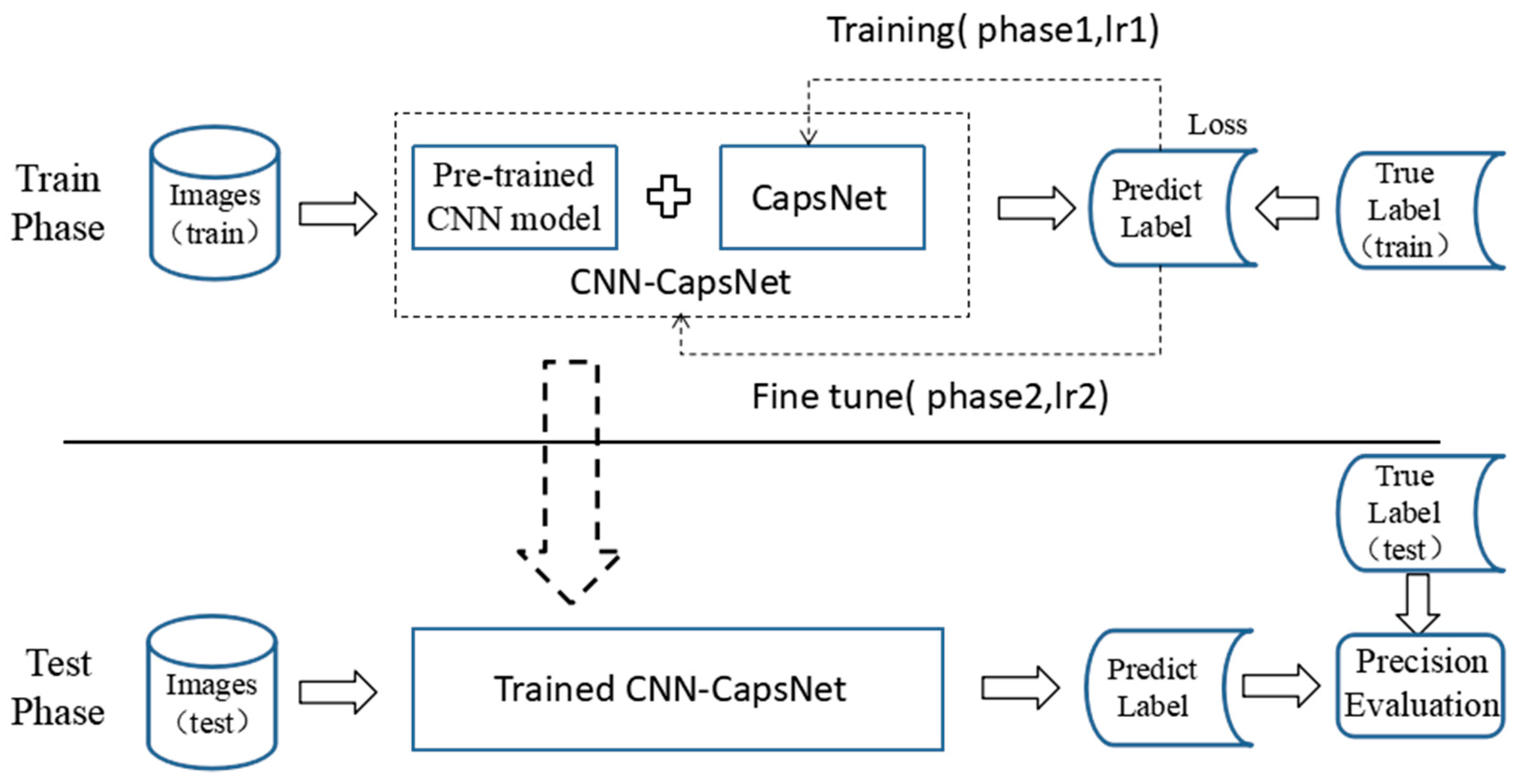
As shown in Figure 11, the proposed method includes two training phases. In the first training phase, the parameters in the pretrained CNN model are frozen, and weights in the CapsNet are initialized by Gaussian distribution with zero mean and unit variance. Then, they are trained with a learning rate of lr1 to minimize the sum of the margin losses in Equation (6). When the CapsNet is fully trained, the second training phase begins with a lower learning rate lr2 to fine-tune the whole architecture until convergence. The parameters between the adjacent capsule layers except for the coupling coefficient can be updated by a gradient descent algorithm, while the coupling coefficients are determined by the iterative dynamic routing algorithm [36]. The optimal routing number in the iterative dynamic routing algorithm is discussed in Section 3.2. When the training finishes, the testing images are fed into the fully trained CNN-CapsNet architecture to evaluate the classification result.
4. Results and Analysis
4.1. Experimental Setup
4.1.1. Implementation Details
In this work, the Keras framework was used to implement the proposed method. The hyperparameters used in the training stage were set by trial and error as follows. For the Adam optimization algorithm, the batch-size was set as 64 and 50 to cater to the computer memory (due to the different volume of training parameters of the model in two training phases); the learning rates lr1 and lr2 were set as 0.001 and 0.0002 separately for two training phases. The sum of all classes’ margin losses in Equation (6) was used for the loss function, and m+, m−, and λ were set as 0.9, 0.1 and 0.5. All models were trained until the training loss converged. At the same time, for a fair comparison, the same ratios were applied in the following experiments according to the experimental settings in works [23,24,25,27,28,30,35,53,54,55,56,57,63,64,65,66,67,68]. For the UC Merced Land-Use dataset, the 80% and 50% training ratio were set separately. For the AID dataset, 50% and 20% of the images were randomly selected as the training samples, and the rest were left for testing. In addition, a 20% and 10% training ratio were used for the NWPU-RESISC45 dataset. Here, two training ratios were considered for each of the three datasets to comprehensively evaluate the proposed method. Moreover, different ratios were used for different datasets because the numbers of images for the three datasets are different. A small ratio can usually satisfy the full training requirement of the models when a dataset has a large amount of data. Note that all images in the AID dataset were resized to 256 × 256 pixel from the original 600 × 600 pixel because of memory overflow in the training phase. All the implementations were evaluated on an Ubuntu 16.04 operating system with one 3.6 GHz 8-core i7-4790CPU and 32GB memory. Additionally, a NVIDIA GTX 1070 graphics processing unit (GPU) was used to accelerate computing.
4.1.2. Evaluation Protocol
The overall accuracy (OA) and confusion matrix were computed to evaluate experimental results and to compare with the state-of-the-art methods. The OA was defined as the number of correctly classified images divided by the total number of test images, which is a valuable measure to reveal the classification method performance on the whole test images. The value of OA is in the range of 0 to 1, and a higher value indicates a better classification performance. The confusion matrix is an informative table that can allow direct visualization of the performance on each class and can be used for easily analyzing the errors and confusion between different classes, in which the column represents the instances in a predicted class and the row represents the instances in an actual class. Thus, each item xij in the matrix is the proportion of images that are predicted to be the i-th class while truly belonging to the j-th class.
To compute the overall accuracy, the dataset was randomly divided into training and testing sets according to the ratios in Section 4.1.1 and repeated ten times to reduce the influence of the randomness for a reliable result. The mean and standard deviation of overall accuracies on the testing sets from each individual run were reported. Additionally, the confusion matrix was obtained from the best classification results by fixing the ratios of the training sets of the UC Merced Land-Use dataset, AID dataset and NWPU-RESISC45 dataset to be 50%, 20%, and 20%, respectively.
4.2. Experimental Results and Analysis
4.2.1. Analysis of Experimental Parameters
In this section, three parameters including the routing number, the dimension of the capsule in the CapsNet, and different pretrained CNN models, were tested to analyze how these parameters affect the classification result. In addition, the optimal parameters used in the experiments of Section 4.2.2 and Section 4.2.3. Training rations of 80%, 50%, 20% were selected for the UC Merced Land-Use dataset, AID dataset and NWPU-RESISC45 dataset, respectively, in this section’s experiments.
1. The routing number
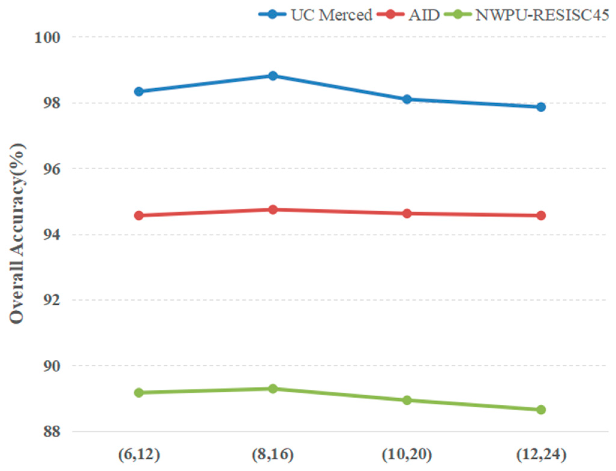
In the dynamic routing algorithm, the routing number is a vital parameter for determining whether the CapsNet can obtain the best coupling coefficients. Therefore, it is necessary to select an optimal routing number. Thus, the routing number was set to (1, 2, 3, 4) while other parameters in the proposed architecture were kept the same. The pretrained VGG-16 model was selected as the primary feature extractor, and the dimension of the capsule in the PrimaryCaps and FinalCaps layers were set to 8 and 16, respectively. As shown in Figure 12, the OAs first increased and then decreased with the increase in the routing number for all three datasets and all reached their peaks at the routing number of 2. A smaller value may generate inadequate training, and a larger value will lead to missing the optimal fitting. In addition, the bigger the value is, the longer the required training time. Comprehensively, the routing number 2 was chosen as the optimal number, considering the training time and was applied in remaining experiments.
2. The dimension of the capsule
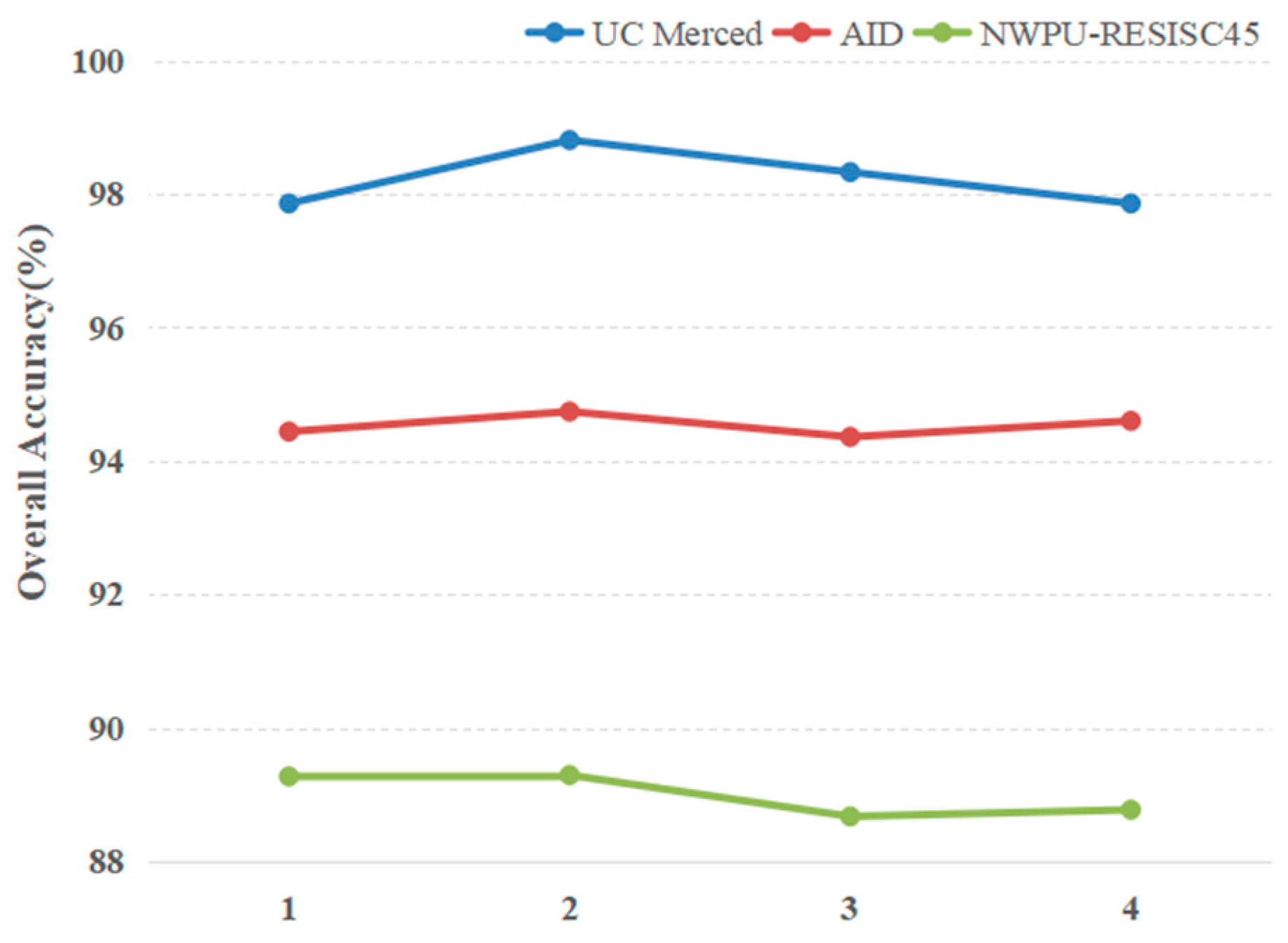
The capsule is the core component of CapsNet and consists of many neurons, and their activities within a capsule represent the various properties of a remote sensing scene image. The primary capsules in the PrimaryCaps are the lower-level capsules that are learned from the primary feature maps extracted from the pretrained CNN models, and they can represent some small entities in the remote sensing image. The capsules with a higher dimension in the FinalCaps are in a higher level and represent more complex entities such as the scene class that the image presents. Thus, the dimension of the capsule in the CapsNet should be considered for its importance in the final classification result. When the dimension of the capsule is low, the representation ability of the capsule is weak, which leads to confusion between two scene classes with high similarity in image context. In contrast, the capsule with a high dimension may contain redundant information or noise, e.g., two neurons may represent very similar properties. Both of them will have a negative influence on the classification result. Thus, a set of values ((6,12), (8,16), (10,20), (12,24)) were set to evaluate the capsule’s influence. Additionally, other parameters were fixed with the pretrained VGG-16 model as the primary feature extractor, and the routing number was set to 2. The experimental results are shown in Figure 13. As expected, in all three datasets, the curves of OAs had their single peaks. The value (8, 16) obtained the best performance, and thus it was used in the next experiments.
3. Different pretrained CNN models
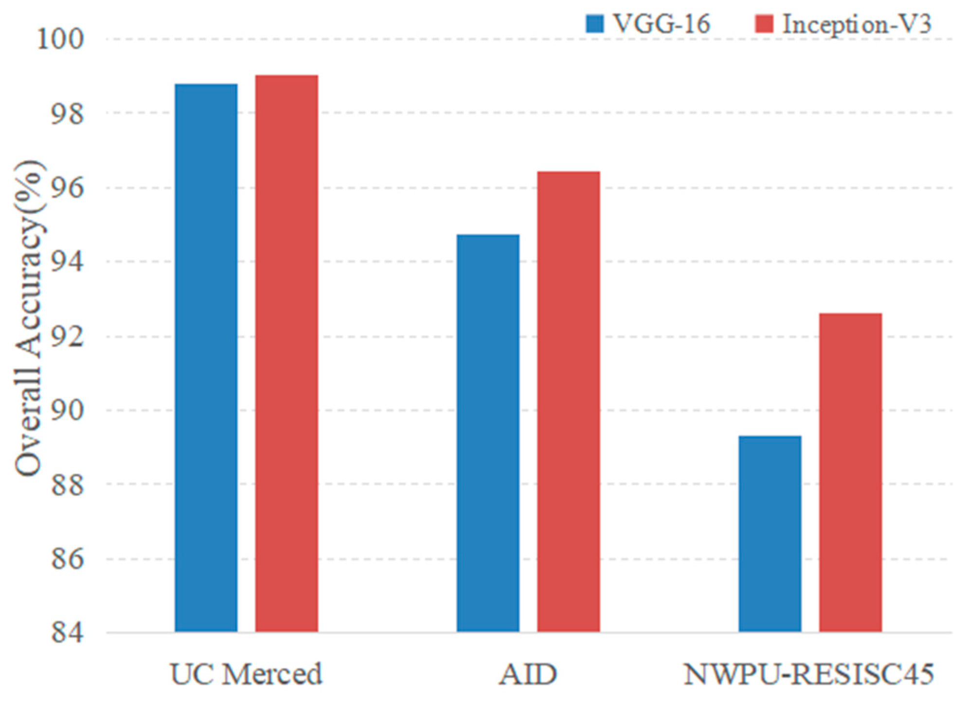
As described in Section 3.3, two representative CNN architectures (VGG-16 and Inception-v3) were selected as feature extractors to evaluate the effectiveness of convolutional features on classification. The “block4_pool” layer of VGG-16 and the “mixd7” of Inception-V3 were selected as the layer of initial feature maps. Other parameters remained unchanged in the experiment. As shown in Figure 14, the Inception-v3 model achieved the highest classification accuracy on all three datasets. This can be explained by the fact that the Inception-v3 consists of the inception modules, which can extract multiscale features and have a stronger ability to extract effective features than VGG-16; however, compared with the Inception-v3, the VGG-16 may lose considerable information due to the consistent existence of pooling layers. Moreover, the OA differences between VGG-16 and Inception-v3 on the AID and NWPU-RESISC45 datasets were more conspicuous than those on the UC Merced dataset.
Compared with the UC Merced dataset, the other two datasets have more classes, higher intraclass variations and smaller interclass dissimilarity. Since the Inception-v3 shows its effectiveness in extracting features with more complex datasets, it was chosen as the final feature extractor on the evaluation of the proposed method.
4.2.2. Experimental Results
1. Classification of the UC Merced Land-Use dataset
To evaluate the classification performance of the proposed method, a comparative evaluation against several state-of-the-art classification methods on the UC Merced Land-Use dataset is shown in Table 1. As seen from Table 1, the proposed architecture CNN-CapsNet using pretrained Inception-v3 as the initial feature maps extractor (denoted as Inception-v3-CapsNet) achieved the highest OA of 99.05% and 97.59% for 80% and 50% training ratio, respectively, among all methods. The CNN-CapsNet using pretrained VGG-16 as the initial feature maps extractor (denoted as VGG-16-CapsNet) also outperformed most methods. This demonstrates that the CNN-CapsNet architecture can learn a higher level representation of scene images by combining CNN and CapsNet.
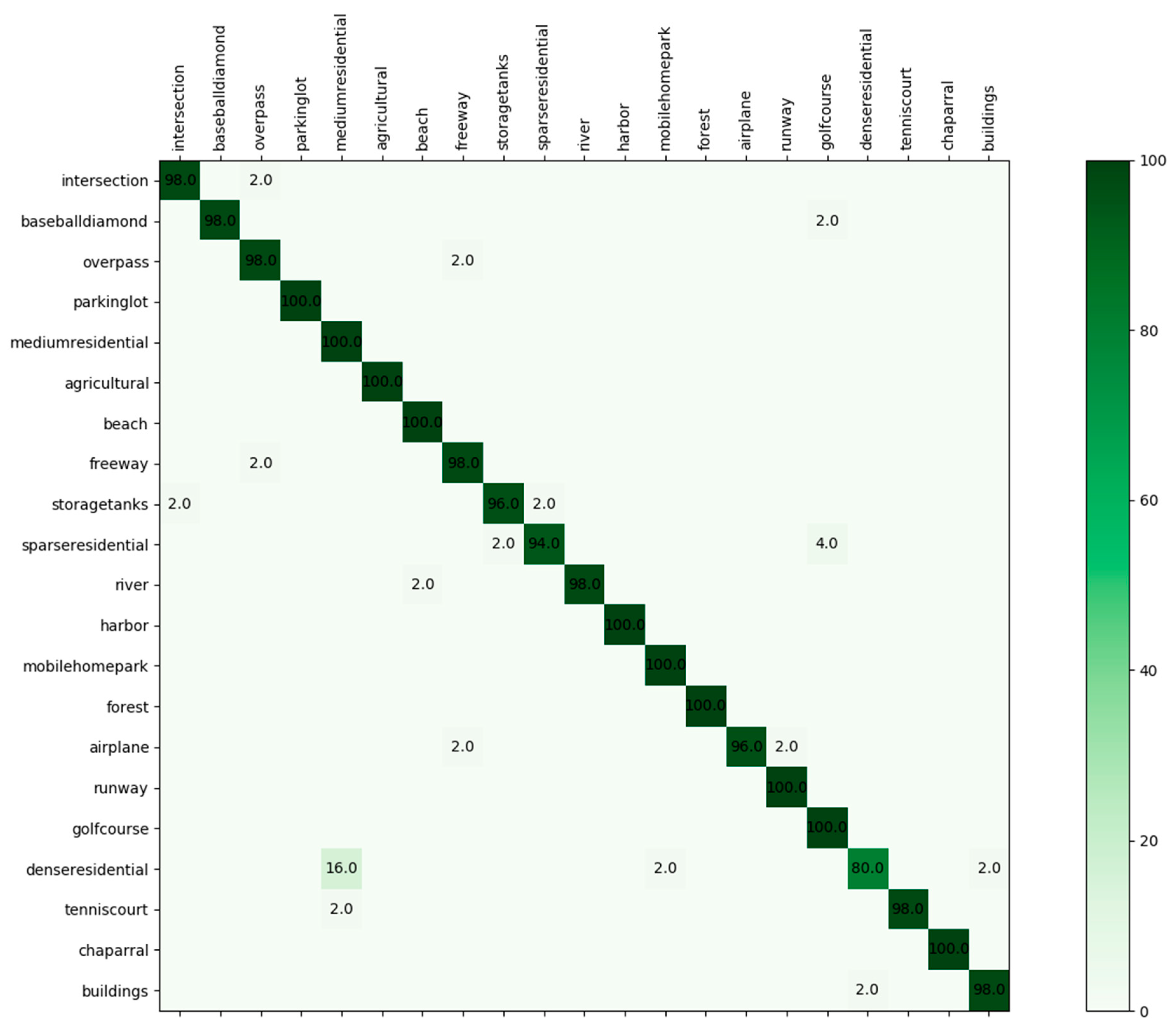
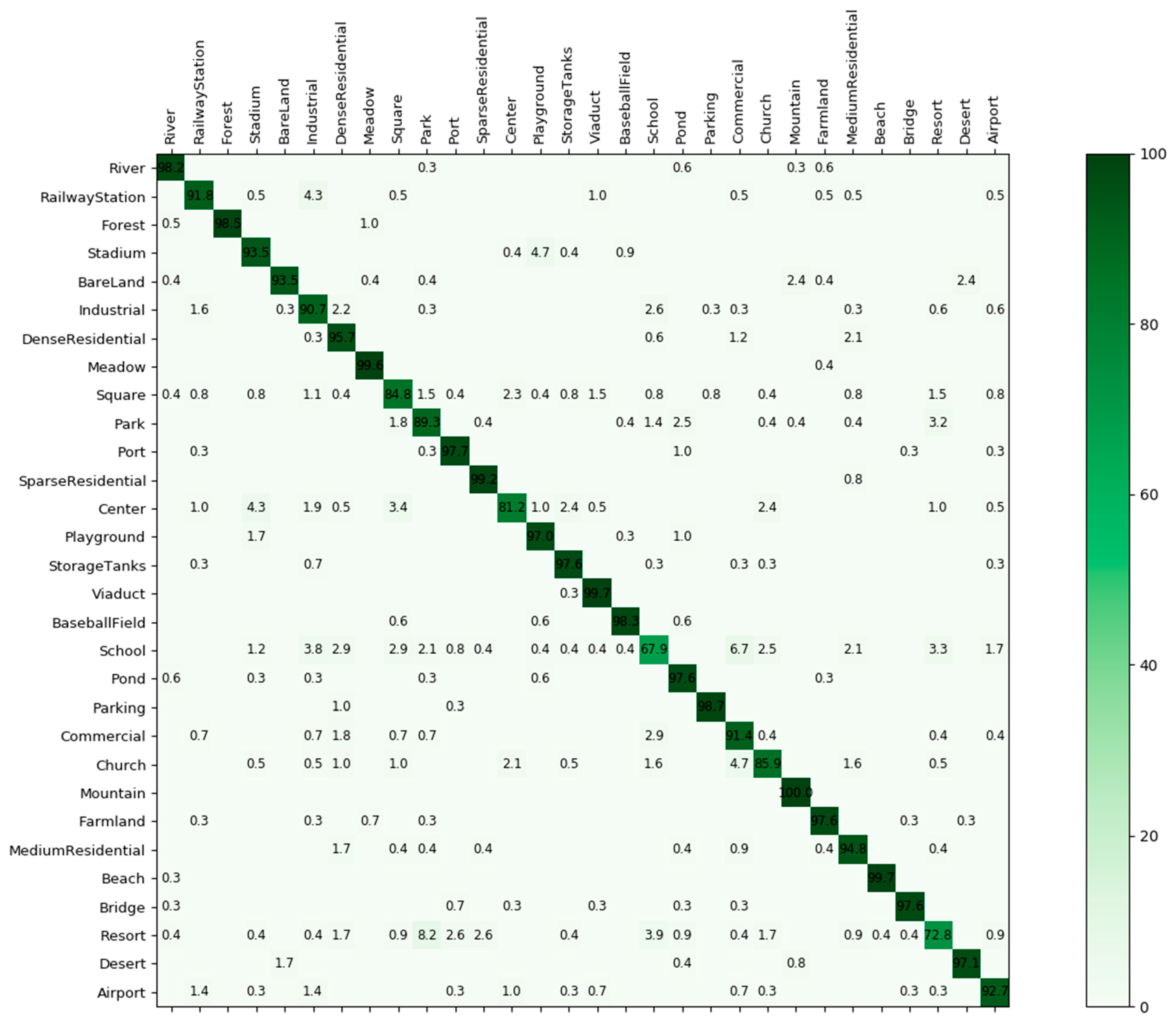
Figure 15 shows the confusion matrix generated from the best classification result by Inception-v3-CapsNet with the training ratio of 50%. As shown in the confusion matrix, 20 categories achieved accuracies greater than 94%, half of which achieved an accuracy of 100%. In addition, only the class of ‘dense residential’, which were easily confused with ‘medium residential’, achieved an accuracy of 80%. This may have resulted from the fact that the two classes have similar image distributions, such as the building structure and density which cannot be well utilized to distinguish each other.
2. Classification of AID dataset
The AID dataset was also tested to demonstrate the effectiveness of the proposed method, compared with other state-of-the-art methods on the same dataset. The results are shown in Table 2. It can be seen that the proposed method of the Inception-v3-CapsNet model generated the best performance with OAs of 96.32% and 93.79% by using 50% and 20% samples, respectively, for training, except for approximately 0.53% lower performance than the method of GCFs + LOFs in a 50% training ratio. This can be explained that the process of downsampling from 600 × 600 to 256 × 256 for the AID dataset in the preprocessing causes some loss of important information and has a negative effect on the classification result. However, in the 20% training ratio, the proposed method outperforms GCFs + LOFs by approximately 1.31%. In addition, data augmentation was used in GCFs + LOFs. Thus, overall, the proposed method yields the state-of-the-art result on AID dataset comprehensively.
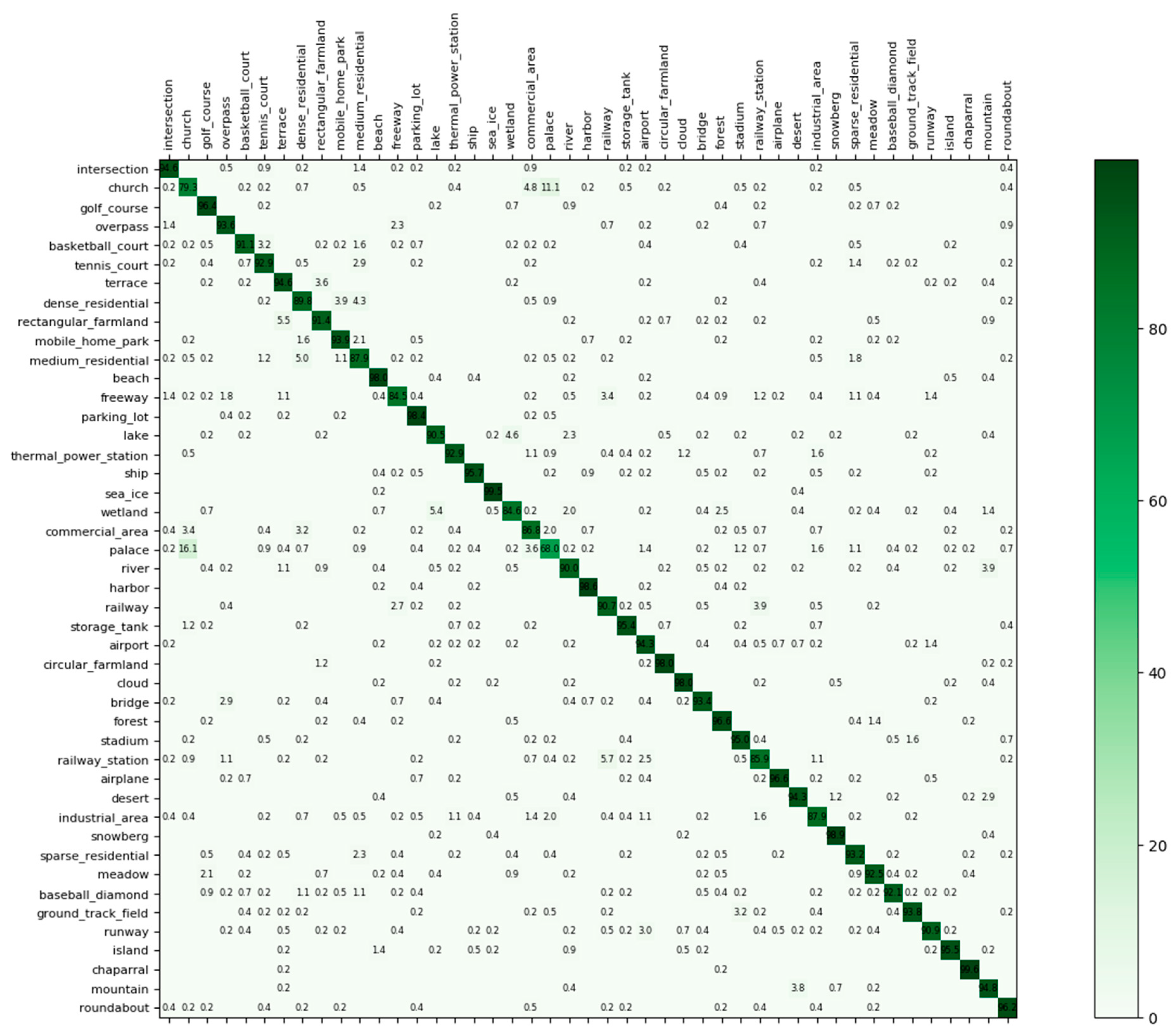
As for the analysis of the confusion matrix, shown in Figure 16, 80% of all 30 categories achieved classification accuracies greater than 90% where the mountain class achieved the 100% accuracy. Some categories with small interclass dissimilarity, such as ’sparse residential’, ‘medium residential’, and ‘dense residential’ were also classified accurately with 99.17%, 94.83% and 95.73%, respectively. The classes of ‘school’ and ‘resort’ had relatively low classification accuracies with 67.92% and 72.84. In detail, the ‘school’ class was easily confused with ‘commercial’ because they had the same image distribution. In addition, the resort class was usually misclassified as ‘park’ due to the existence of some analogous objects such as green belts and ponds. Even so, great improvements were achieved by the proposed method, compared with the classification accuracy of 49% and 60% in [35]. This means that the CNN-CapsNet could learn the differences of spatial information between these scene classes with the same image distribution and distinguish them effectively.
3. Classification of NWPU-RESISC45 dataset
Table 3 shows the classification performance comparison of the proposed architecture and the existing state-of-the-art methods using the most challenging NWPU-RESISC45 dataset. It can be observed that the Inception-v3-CapsNet model also achieved remarkable classification results, with OA improvements of 0.27% and 1.88% over the second best model using 20% and 10% training ratios, respectively. The good performance of the proposed method further verifies the effectiveness of combining the pretrained CNN model and CapsNet.
Figure 17 gives the confusion matrix generated from the best classification result by Inception-v3-CapsNet with the training ratio of 20%. From the confusion matrix, 36 categories among all 45 categories achieved classification accuracies greater than 90%. The major confusion was in ‘palace’ and ‘church’ because both of them have similar styles of buildings. In spite of that, substantial improvements were still achieved with 79.3% and 68% compared with 75% and 64% in [53], respectively.
4.2.3. Further Explanation
In Section 4.2.2, it was found that the proposed method obtains state-of-the-art classification results. This mainly benefits from the following three factors: fine-tuning, capsules and the pretrained CNN model. In this section, further analysis will be performed on how they accomplish the significant performance for classification. In addition, the training ratios of the three datasets were the same as those in Section 4.2.1.
1. Effectiveness of fine-tuning
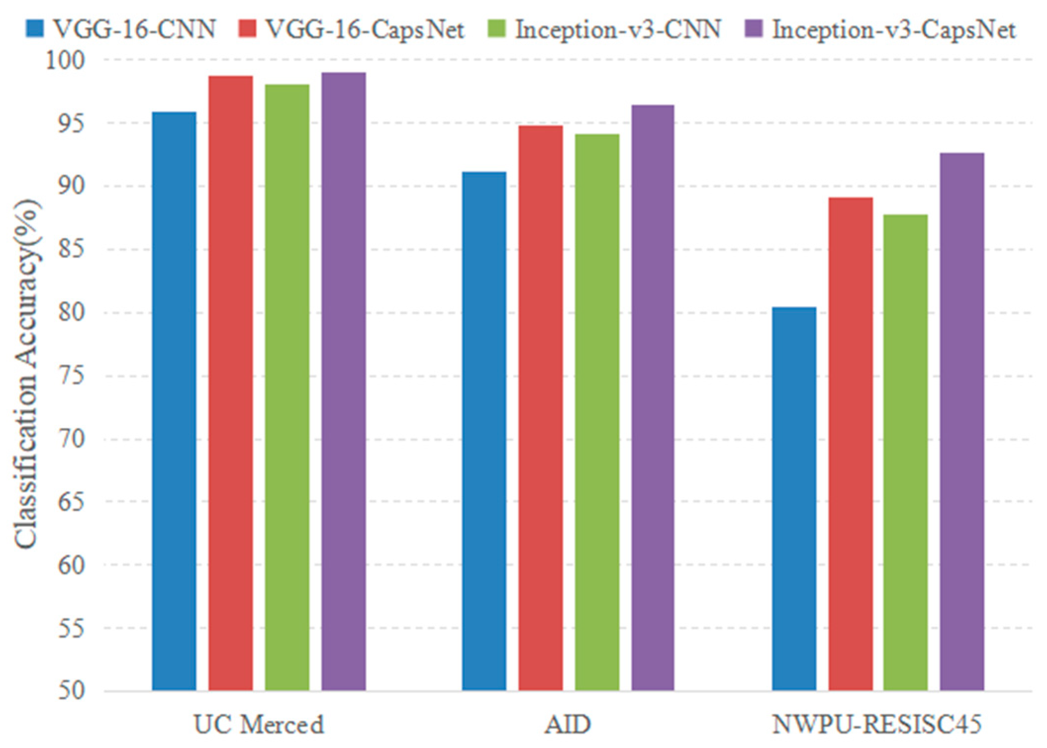
First, the strategy of fine-tuning was added to train the proposed architecture. To evaluate the effectiveness of fine-tuning in the proposed method, a comparison was made between the classification results with and without fine-tuning. As shown in Figure 18, the methods with fine-tuning obtained a significant improvement compared with no fine-tuning operation. The reason is that the features extracted from the pretrained CNN models have a strong relationship with the original task. Fine-tuning can adjust the parameters of the pretrained CNN model to cater to the current training datasets for an accuracy improvement.
2. Effectiveness of capsules
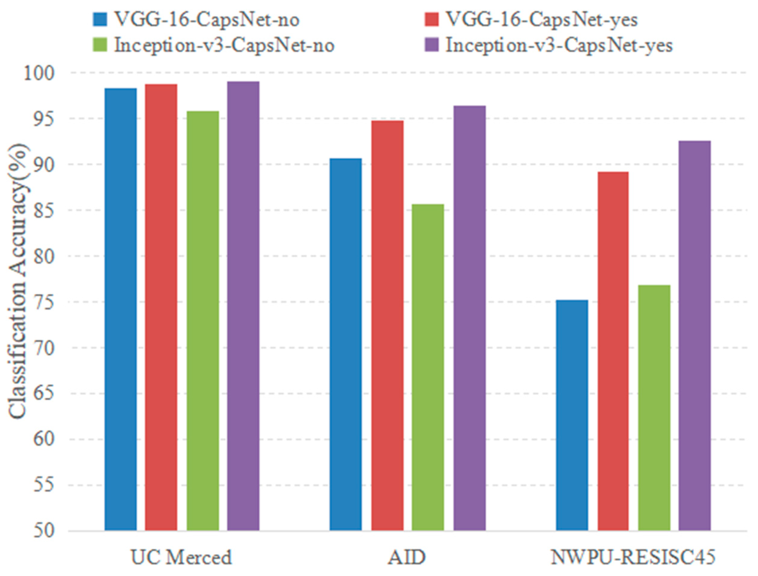
In the design of the proposed architecture, the CapsNet is used as the classifier to label the remote sensing image, which uses the capsule to replace the neuron in traditional neural networks. To prove the validity of the positive impact on classification results with this replacement, a comparative experiment was conducted. In detail, a new CNN architecture was designed as the classifier, which consists of one convolutional layer and two fully connected layers. In addition, the only difference between the new CNN architecture and the CapsNet described in Section 3.3 was using the neuron to replace the capsule while other parameters including the training hyperparameters were all kept the same. The experimental results are shown in Figure 19 (the VGG-16-CNN and Inception-v3-CNN in Figure 19 mean that using pretrained VGG-16 and Inception-v3 as feature extractors, respectively, and using the newly designed CNN architecture as the classifier). For three datasets, the models using capsules all achieved better performance than those using traditional neurons. This further demonstrates that the CapsNet can learn more representative information of scene images.
3. Effectiveness of the pretrained CNN model
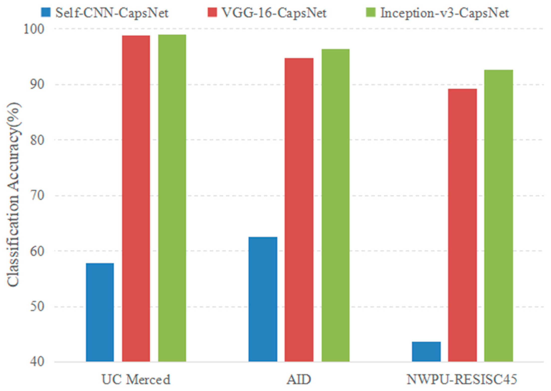
The pretrained CNN model was selected as the initial feature maps extractor instead of designing a new CNN architecture. This is also a great factor for the success of the proposed architecture. For comparison, a CNN architecture (Self-CNN) was designed, which only contained four consecutive convolutional layers and the size of its output feature maps was 16 × 16 × 512, the same as that of the pretrained VGG-16 used in this paper. The parameters of the CapsNet were the same. The new Self-CNN-CapsNet architecture was trained from scratch. The classification results are presented in Figure 20. From the Figure, the classification accuracy of CNN-CapsNet with the pretrained CNN model as the feature extractor was much higher than that with self-CNN. This is because the existing datasets cannot fully train the model and further proves the effectiveness of using pretrained CNN models as feature extractors.
5. Conclusions
In recent years, the prevalence of deep learning methods especially the CNN has made the performance of remote sensing scene classification state-of-the-art. However, the scene classes with the same image distribution are still not distinguished effectively. This is mainly because some fully connected layers are added to the end of the CNN, which gives less consideration to the spatial relationship that is vital to classification. To preserve the spatial information, the new architecture CapsNet is proposed, which uses the capsule to replace the neuron in the traditional neural network. In addition, the capsule is a vector to represent internal properties that can be used to learn part-whole relationships within an image. In this paper, to further improve the classification accuracy of remote sensing image scene classification and inspired by the CapsNet, a novel architecture named CNN-CapsNet is proposed for remote sensing image scene classification. The proposed architecture consists of two parts: CNN and CapsNet. The CNN part is transferring the original remote sensing images to the original feature maps. In addition, the CapsNet part converts the original feature maps into various levels of capsules and to obtain the final classification result. Experiments were performed on three public challenging datasets, and the experimental results demonstrate the effectiveness of the proposed CNN-CapsNet and show that the proposed method outperforms the current state-of-the-art methods. In future work, different from using feature maps from only one CNN model, in this paper, feature maps from different pretrained CNN models will be merged for remote sensing image scene classification.
Author Contributions
W.Z. conceived and designed the whole framework and the experiments, as well as wrote the manuscript. L.Z. contributed to the discussion of the experimental design. L.Z. and P.T. all helped to organize the paper and performed the experimental analysis. P.T. helped to revise the manuscript, and all authors read and approved the submitted manuscript.
Acknowledgments
This research was funded by the National Natural Science Foundation of China under grant 41701397; and the Major Project of High-Resolution Earth Observation System of China under Grant 03-Y20A04-9001-17/18.
Conflicts of Interest
The authors declare no conflict of interest.
References
- Plaza, A.; Plaza, J.; Paz, A.; Sanchez, S. Parallel hyperspectral image and signal processing. IEEE Signal Process. Mag. 2011, 28, 119–126. [Google Scholar] [CrossRef]
- Hubert, M.J.; Carole, E. Airborne SAR-efficient signal processing for very high resolution. Proc. IEEE 2013, 101, 784–797. [Google Scholar] [CrossRef]
- Cheriyadat, A.M. Unsupervised feature learning for aerial scene classification. IEEE Trans. Geosci. Remote Sens. 2014, 52, 439–451. [Google Scholar] [CrossRef]
- Shao, W.; Yang, W.; Xia, G.S. Extreme value theory-based calibration for the fusion of multiple features in high-resolution satellite scene classification. Int. J. Remote Sens. 2013, 34, 8588–8602. [Google Scholar] [CrossRef]
- Estoque, R.C.; Murayama, Y.; Akiyama, C.M. Pixel-based and object-based classifications using high- and medium-spatial-resolution imageries in the urban and suburban landscapes. Geocarto Int. 2015, 30, 1113–1129. [Google Scholar] [CrossRef]
- Zhang, X.; Wang, Q.; Chen, G.; Dai, F.; Zhu, K.; Gong, Y.; Xie, Y. An object-based supervised classification framework for very-high-resolution remote sensing images using convolutional neural networks. Remote Sens. Lett. 2018, 9, 373–382. [Google Scholar] [CrossRef]
- Yang, Y.; Newsam, S. Comparing SIFT descriptors and Gabor texture features for classification of remote sensed imagery. In Proceedings of the 15th IEEE International Conference on Image Processing (ICIP), San Diego, CA, USA, 12–15 October 2008; pp. 1852–1855. [Google Scholar]
- Dos Santos, J.A.; Penatti, O.A.B.; da Silva Torres, R. Evaluating the Potential of Texture and Color Descriptors for Remote Sensing Image Retrieval and Classification. In Proceedings of the VISAPP, Angers, France, 17–21 May 2010; pp. 203–208. [Google Scholar]
- Chen, C.; Zhang, B.; Su, H.; Li, W.; Wang, L. Land-use scene classification using multi-scale completed local binary patterns. Signal Image Video Process. 2016, 10, 745–752. [Google Scholar] [CrossRef]
- Li, H.T.; Gu, H.Y.; Han, Y.S.; Yang, J.H. Object oriented classification of high-resolution remote sensing imagery based on an improved colour structure code and a support vector machine. Int. J. Remote Sens. 2010, 31, 1453–1470. [Google Scholar] [CrossRef]
- Penatti, O.A.; Nogueira, K.; dos Santos, J.A. Do deep features generalize from everyday objects to remote sensing and aerial scenes domains? In Proceedings of the IEEE Conference on Computer Vision and Pattern Recognition Workshops, Boston, MA, USA, 7–12 June 2015; pp. 44–51. [Google Scholar]
- Luo, B.; Jiang, S.J.; Zhang, L.P. Indexing of remote sensing images with different resolutions by multiple features. IEEE J. Sel. Top. Appl. Earth Obs. Remote Sens. 2013, 6, 1899–1912. [Google Scholar] [CrossRef]
- Zhou, L.; Zhou, Z.; Hu, D. Scene classification using a multi-resolution bag-of-features model. Pattern Recognit. 2013, 46, 424–433. [Google Scholar] [CrossRef]
- Yang, Y.; Newsam, S. Bag-of-visual-words and spatial extensions for land-use classification. In Proceedings of the 18th SIGSPATIAL International Conference on Advances in Geographic Information Systems, San Jose, CA, USA, 3–5 November 2010; pp. 270–279. [Google Scholar]
- Zhao, L.; Tang, P.; Huo, L. A 2-D wavelet decomposition-based bag-of-visual-words model for land-use scene classification. Int. J. Remote Sens. 2014, 35, 2296–2310. [Google Scholar] [CrossRef]
- Zhao, L.; Tang, P.; Huo, L. Land-use scene classification using a concentric circle-structured multiscale bag-of-visual-words model. IEEE J. Sel. Top. Appl. Earth Obs. Remote Sens. 2014, 7, 4620–4631. [Google Scholar] [CrossRef]
- Sridharan, H.; Cheriyadat, A. Bag of lines (bol) for improved aerial scene representation. IEEE Geosci. Remote Sens. Lett. 2015, 12, 676–680. [Google Scholar] [CrossRef]
- Zhu, Q.; Zhong, Y.; Zhao, B.; Xia, G.; Zhang, L. Bag-of-visual-words scene classifier with local and global features for high spatial resolution remote sensing imagery. IEEE Geosci. Remote Sens. Lett. 2016, 13, 747–751. [Google Scholar] [CrossRef]
- He, K.M.; Zhang, X.Y.; Ren, S.Q.; Sun, J. Deep residual learning for image recognition. In Proceedings of the 2016 IEEE Conference on Computer Vision and Pattern Recognition (CVPR), Las Vegas, NV, USA, 26–30 June 2016; pp. 770–778. [Google Scholar] [CrossRef]
- Girshick, R.; Donahue, J.; Darrell, T.; Malik, J. Rich feature hierarchies for accurate object detection and semantic segmentation. In Proceedings of the 2014 IEEE Conference on Computer Vision and Pattern Recognition (CVPR), Ohio, CO, USA, 24–27 June 2014; pp. 580–587. [Google Scholar] [CrossRef]
- Long, J.; Shelhamer, E.; Darrell, T. Fully convolutional networks for semantic segmentation. In Proceedings of the 2015 IEEE Conference on Computer Vision and Pattern Recognition (CVPR), Boston, MA, USA, 7–12 June 2015; pp. 3431–3440. [Google Scholar] [CrossRef]
- Zhong, Y.; Fei, F.; Zhang, L. Large patch convolutional neural networks for the scene classification of high spatial resolution imagery. J. Appl. Remote Sens. 2016, 10, 025006. [Google Scholar] [CrossRef]
- Zhang, F.; Du, B.; Zhang, L. Scene classification via a gradient boosting random convolutional network ramework. IEEE Trans. Geosci. Remote Sens. 2016, 54, 1793–1802. [Google Scholar] [CrossRef]
- Liu, Y.; Zhong, Y.; Fei, F.; Zhu, Q.; Qin, Q. Scene Classification Based on a Deep Random-Scale Stretched Convolutional Neural Network. Remote Sens. 2018, 10, 444. [Google Scholar] [CrossRef]
- Castelluccio, M.; Poggi, G.; Sansone, C.; Verdoliva, L. Land use classification in remote sensing images by convolutional neural networks. arXiv, 2015; arXiv:1508.00092. [Google Scholar]
- Nogueira, K.; Penatti, O.A.B.; dos Santos, J.A. Towards better exploiting convolutional neural networks for remote sensing scene classification. Pattern Recognit. 2017, 61, 539–556. [Google Scholar] [CrossRef] [Green Version]
- Hu, F.; Xia, G.S.; Hu, J.; Zhang, L. Transferring deep convolutional neural networks for the scene classification of high-resolution remote sensing imagery. Remote Sens. 2015, 7, 14680–14707. [Google Scholar] [CrossRef]
- Chaib, S.; Liu, H.; Gu, Y.; Yao, H. Deep feature fusion for VHR remote sensing scene classification. IEEE Trans. Geosci. Remote Sens. 2017, 55, 4775–4784. [Google Scholar] [CrossRef]
- Zou, Q.; Ni, L.; Zhang, T.; Wang, Q. Deep learning based feature selection for remote sensing scene classification. IEEE Geosci. Remote. Sens. Lett. 2015, 12, 2321–2325. [Google Scholar] [CrossRef]
- Yu, Y.; Liu, F. A two-stream deep fusion framework for high-resolution aerial scene classification. Comput. Intell. Neurosci. 2018, 2018, 8639367. [Google Scholar] [CrossRef] [PubMed]
- Othman, E.; Bazi, Y.; Alajlan, N.; Alhichri, H.; Melgani, H. Using convolutional features and a sparse autoencoder for land-use scene classification. Int. J. Remote Sens. 2016, 37, 2149–2167. [Google Scholar] [CrossRef]
- Marmanis, D.; Datcu, M.; Esch, T.; Stilla, U. Deep learning earth observation classification using ImageNet pretrained networks. IEEE Geosci. Remote Sens. Lett. 2016, 13, 105–109. [Google Scholar] [CrossRef]
- Cheng, G.; Ma, C.; Zhou, P.; Yao, X.; Han, J. Scene classification of high resolution remote sensing images using convolutional neural networks. In Proceedings of the IEEE International Geoscience Remote Sensing Symposium (IGARSS), Beijing, China, 10–15 July 2016; pp. 767–770. [Google Scholar] [CrossRef]
- Zhao, L.; Zhang, W.; Tang, P. Analysis of the inter-dataset representation ability of deep features for high spatial resolution remote sensing image scene classification. Multimed. Tools Appl. 2018. [Google Scholar] [CrossRef]
- Xia, G.S.; Hu, J.; Hu, F.; Shi, B.; Bai, X.; Zhong, Y.; Zhang, L.; Lu, X. AID: A benchmark data set for performance evaluation of aerial scene classification. IEEE Trans. Geosci. Remote Sens. 2017, 55, 3965–3981. [Google Scholar] [CrossRef]
- Sabour, S.; Frosst, N.; Hinton, G.E. Dynamic routing between capsules. In Proceedings of the 31st Conference on Neural Information Processing Systems (NIPS), Long Beach, CA, USA, 4–9 December 2017; pp. 3859–3869. [Google Scholar]
- Andersen, P.A. Deep Reinforcement learning using capsules in advanced game environments. arXiv, 2018; arXiv:1801.09597. [Google Scholar]
- Afshar, P.; Mohammadi, A.; Plataniotis, K.N. Brain Tumor Type Classification via Capsule Networks. arXiv, 2018; arXiv:1802.10200. [Google Scholar]
- Iqbal, T.; Xu, Y.; Kong, Q.; Wang, W. Capsule routing for sound event detection. arXiv, 2018; arXiv:1806.04699. [Google Scholar]
- LaLonde, R.; Bagci, U. Capsules for object segmentation. arXiv, 2018; arXiv:1804.04241. [Google Scholar]
- Deng, F.; Pu, S.; Chen, X.; Shi, Y.; Yuan, T.; Pu, S. Hyperspectral Image Classification with Capsule Network Using Limited Training Samples. Sensors 2018, 18, 3153. [Google Scholar] [CrossRef] [PubMed]
- Xi, E.; Bing, S.; Jin, Y. Capsule Network Performance on Complex Data. arXiv, 2017; arXiv:1712.03480. [Google Scholar]
- Jaiswal, A.; AbdAlmageed, W.; Natarajan, P. CapsuleGAN: Generative adversarial capsule network. arXiv, 2018; arXiv:1802.06167. [Google Scholar]
- Neill, J.O. Siamese capsule networks. arXiv, 2018; arXiv:1805.07242. [Google Scholar]
- Mobiny, A.; Nguyen, H.V. Fast CapsNet for lung cancer screening. arXiv, 2018; arXiv:1806.07416. [Google Scholar]
- Kumar, A.D. Novel Deep learning model for traffic sign detection using capsule networks. arXiv, 2018; arXiv:1805.04424. [Google Scholar]
- Li, Y.; Qian, M.; Liu, P.; Cai, Q.; Li, X.; Guo, J.; Yan, H.; Yu, F.; Yuan, K.; Yu, J.; et al. The recognition of rice images by UAV based on capsule network. Clust. Comput. 2018. [Google Scholar] [CrossRef]
- Qiao, K.; Zhang, C.; Wang, L.; Yan, B.; Chen, J.; Zeng, L.; Tong, L. Accurate reconstruction of image stimuli from human fMRI based on the decoding model with capsule network architecture. arXiv, 2018; arXiv:1801.00602. [Google Scholar]
- Zhao, W.; Ye, J.; Yang, M.; Lei, Z.; Zhang, S.; Zhao, Z. Investigating capsule networks with dynamic routing for text classification. arXiv, 2018; arXiv:1804.00538. [Google Scholar]
- Xiang, C.; Zhang, L.; Tang, Y.; Zou, W.; Xu, C. MS-CapsNet: A novel multi-scale capsule network. IEEE Signal Process. Lett. 2018, 25, 1850–1854. [Google Scholar] [CrossRef]
- Simonyan, K.; Zisserman, A. Very deep convolutional networks for large-scale image recognition. In Proceedings of the 2015 International Conference on Learning Representations (ICLR), San Diego, CA, USA, 7–9 May 2015; pp. 1–14. [Google Scholar]
- Russakovsky, A.; Deng, J.; Su, H. ImageNet large scale visual recognition challenge. Int. J. Comput. Vis. 2015, 115, 211–252. [Google Scholar] [CrossRef]
- Cheng, G.; Han, J.; Lu, X. Remote sensing image scene classification: Benchmark and state of the art. Proc. IEEE 2017, 105, 1865–1883. [Google Scholar] [CrossRef]
- Gong, X.; Xie, Z.; Liu, Y.; Shi, X.; Zheng, Z. Deep salient feature based anti-noise transfer network for scene classification of remote sensing imagery. Remote Sens. 2018, 10, 410. [Google Scholar] [CrossRef]
- Chen, G.; Zhang, X.; Tan, X.; Cheng, Y.F.; Dai, F.; Zhu, K.; Gong, Y.; Wang, Q. Training small networks for scene classification of remote sensing images via knowledge distillation. Remote Sens. 2018, 10, 719. [Google Scholar] [CrossRef]
- Zeng, D.; Chen, S.; Chen, B.; Li, S. Improving remote sensing scene classification by integrating global-context and local-object features. Remote Sens. 2018, 10, 734. [Google Scholar] [CrossRef]
- Chen, J.; Wang, C.; Ma, Z.; Chen, J.; He, D.; Ackland, S. Remote sensing scene classification based on convolutional neural networks pre-trained using attention-guided sparse filters. Remote Sens. 2018, 10, 290. [Google Scholar] [CrossRef]
- Zou, J.; Li, W.; Chen, C.; Du, Q. Scene classification using local and global features with collaborative representation fusion. Inf. Sci. 2018, 348, 209–226. [Google Scholar] [CrossRef]
- Mahdianpari, M.; Salehi, B.; Rezaee, M.; Mohammadimanesh, F.; Zhang, Y. Very Deep Convolutional Neural Networks for Complex Land Cover Mapping Using Multispectral Remote Sensing Imagery. Remote Sens. 2018, 10, 1119. [Google Scholar] [CrossRef]
- Krizhevsky, A.; Sutskever, I.; Hinton, G.E. ImageNet classification with deep convolutional neural networks. In Proceedings of the 26th Annual Conference on Neural Information Processing Systems, Harrahs and Harveys, Lake Tahoe, CA, USA, 3–8 December 2012; NIPS Foundation: La Jolla, CA, USA, 2012. [Google Scholar]
- Szegedy, C.; Liu, W.; Jia, Y. Going deeper with convolutions. In Proceedings of the 2015 IEEE Conference on Computer Vision and Pattern Recognition (CVPR), Boston, MA, USA, 7–12 June 2015; pp. 1–9. [Google Scholar] [CrossRef]
- Szegedy, C.; Vanhoucke, V.; Ioffe, S.; Shlens, J. Rethinking the inception architecture for computer vision. arXiv, 2015; arXiv:1512.00567. [Google Scholar]
- Bian, X.; Chen, C.; Tian, L.; Du, Q. Fusing local and global features for high-resolution scene classification. IEEE J. Sel. Top. Appl. Earth Obs. Remote Sens. 2017, 10, 2889–2901. [Google Scholar] [CrossRef]
- Anwer, R.M.; Khan, F.S.; van deWeijer, J.; Monlinier, M.; Laaksonen, J. Binary patterns encoded convolutional neural networks for texture recognition and remote sensing scene classification. arXiv, 2017; arXiv:1706.01171. [Google Scholar] [CrossRef]
- Weng, Q.; Mao, Z.; Lin, J.; Guo, W. Land-Use Classification via Extreme Learning Classifier Based on Deep Convolutional Features. IEEE Geosci. Remote Sens. Lett. 2017, 14, 704–708. [Google Scholar] [CrossRef]
- Qi, K.; Guan, Q.; Yang, C.; Peng, F.; Shen, S.; Wu, H. Concentric Circle Pooling in Deep Convolutional Networks for Remote Sensing Scene Classification. Remote Sens. 2018, 10, 934. [Google Scholar] [CrossRef]
- Cheng, G.; Li, Z.; Yao, X.; Li, K.; Wei, Z. Remote Sensing Image Scene Classification Using Bag of Convolutional Features. IEEE Geosci. Remote Sens. Lett. 2017, 14, 1735–1739. [Google Scholar] [CrossRef]
- Liu, Y.; Huang, C. Scene classification via triplet networks. IEEE J. Sel. Top. Appl. Earth Obs. Remote Sens. 2018, 11, 220–237. [Google Scholar] [CrossRef]
Figure 1.
Sample images labelled school and dense residential in the AID dataset.

Figure 2.
Example images of UC Merced Land-Use dataset: (1) agriculture; (2) airplane; (3) baseball diamond; (4) beach; (5) buildings; (6) chaparral; (7) dense residential; (8) forest; (9) freeway; (10) golf course; (11) harbor; (12) intersection; (13) medium residential; (14) mobile home park; (15) overpass; (16) parking lot; (17) river; (18) runway; (19) sparse residential; (20) storage tanks; and (21) tennis court.

Figure 3.
Example images of AID dataset: (1) airport; (2) bare land; (3) baseball field; (4) beach; (5) bridge; (6) centre; (7) church; (8) commercial; (9) dense residential; (10) desert; (11) farmland; (12) forest; (13) industrial; (14) meadow; (15) medium residential; (16) mountain; (17) park; (18) parking; (19) playground; (20) pond; (21) port; (22) railway station; (23) resort; (24) river; (25) school; (26) sparse residential; (27) square; (28) stadium; (29) storage tanks; and (30) viaduct.


Figure 4.
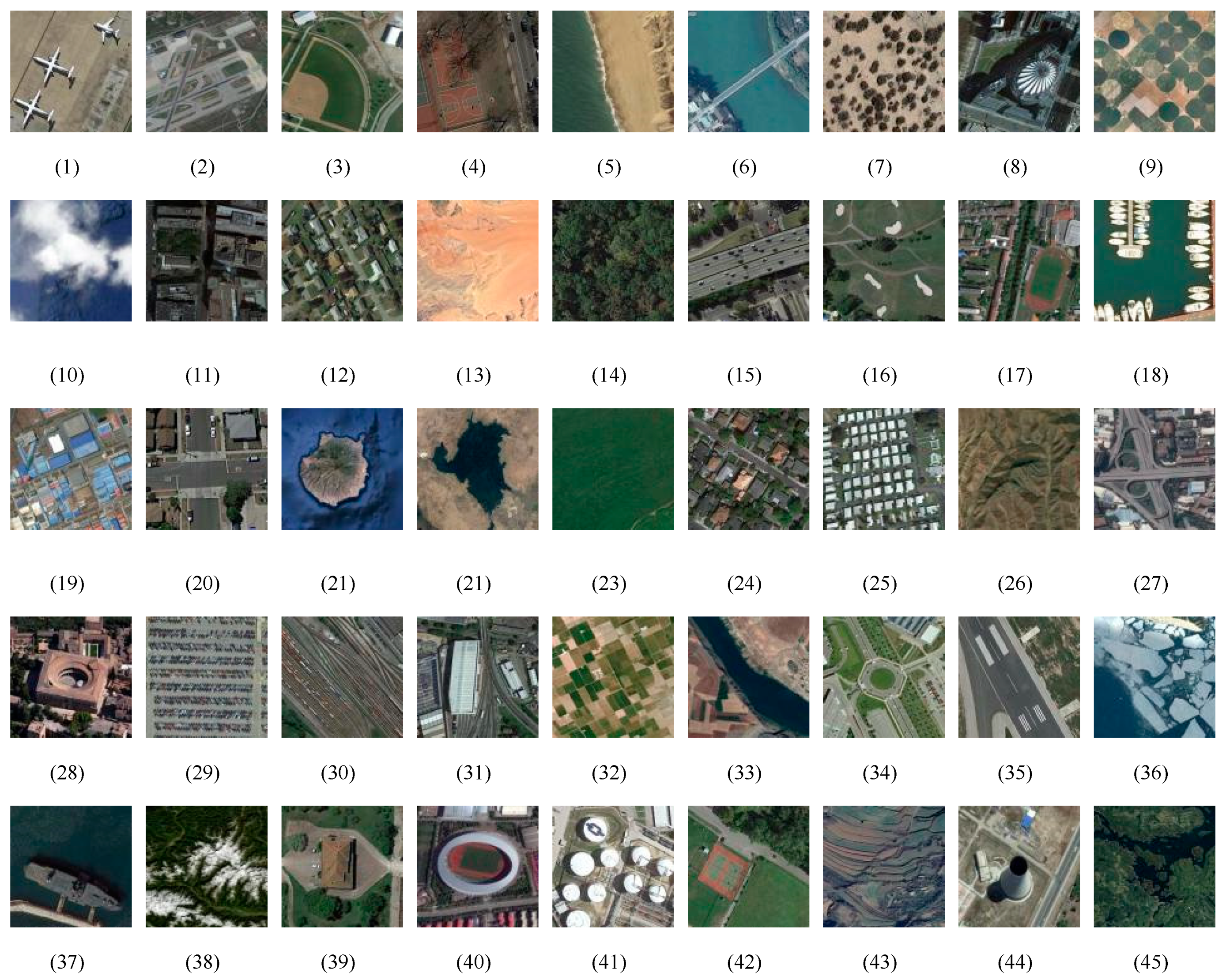
Example images of NWPU-RESISC45 dataset: (1) airplane; (2) airport; (3) baseball diamond; (4) basketball court; (5) beach; (6) bridge; (7) chaparral; (8) church; (9) circular farmland; (10) cloud; (11) commercial area; (12) dense residential; (13) desert; (14) forest; (15) freeway; (16) golf course; (17) ground track field; (18) harbor; (19) industrial area; (20) intersection; (21) island; (22) lake; (23) meadow; (24) medium residential; (25) mobile home park; (26) mountain; (27) overpass; (28) palace; (29) parking lot; (30) railway; (31) railway station; (32) rectangular farmland; (33) river; (34) roundabout; (35) runway; (36) sea ice; (37) ship; (38) snow berg; (39) sparse residential; (40) stadium; (41) storage tank; (42) tennis court; (43) terrace; (44) thermal power station; and (45) wetland.
Figure 4.
Example images of NWPU-RESISC45 dataset: (1) airplane; (2) airport; (3) baseball diamond; (4) basketball court; (5) beach; (6) bridge; (7) chaparral; (8) church; (9) circular farmland; (10) cloud; (11) commercial area; (12) dense residential; (13) desert; (14) forest; (15) freeway; (16) golf course; (17) ground track field; (18) harbor; (19) industrial area; (20) intersection; (21) island; (22) lake; (23) meadow; (24) medium residential; (25) mobile home park; (26) mountain; (27) overpass; (28) palace; (29) parking lot; (30) railway; (31) railway station; (32) rectangular farmland; (33) river; (34) roundabout; (35) runway; (36) sea ice; (37) ship; (38) snow berg; (39) sparse residential; (40) stadium; (41) storage tank; (42) tennis court; (43) terrace; (44) thermal power station; and (45) wetland.

Figure 5.
The convolutional neural network (CNN) architecture.

Figure 6.
Connections between the lower level and higher level capsules.

Figure 7.
A typical CapsNet architecture.

Figure 8.
The detail of FinalCaps.

Figure 9.
The architecture of the proposed classification method.

Figure 10.
Inception-v1 module.

Figure 11.
The flowchart of the proposed method.

Figure 12.
The influence of the routing number on the classification accuracy.

Figure 13.
The influence of the dimension of the capsule on the classification accuracy.

Figure 14.
The influence of pretrained CNN models on the classification accuracy.

Figure 15.
Confusion matrix of the proposed method on UC Merced Land-Use dataset by fixing the training ratio to 50%.
Figure 15.
Confusion matrix of the proposed method on UC Merced Land-Use dataset by fixing the training ratio to 50%.

Figure 16.
Confusion matrix of the proposed method on the AID dataset by fixing the training ratio as 20%.
Figure 16.
Confusion matrix of the proposed method on the AID dataset by fixing the training ratio as 20%.

Figure 17.
Confusion matrix of the proposed method on the NWPU-RESISC45 dataset by fixing the training ratio as 20%.
Figure 17.
Confusion matrix of the proposed method on the NWPU-RESISC45 dataset by fixing the training ratio as 20%.

Figure 18.
Overall accuracy (%) of the proposed method with and without fine-tuning on three datasets.
Figure 18.
Overall accuracy (%) of the proposed method with and without fine-tuning on three datasets.

Figure 19.
Overall accuracy (%) of the proposed method with neuron and capsule on three datasets.

Figure 20.
Overall accuracy (%) of the proposed method with the pretrained model and self-model on three datasets.
Figure 20.
Overall accuracy (%) of the proposed method with the pretrained model and self-model on three datasets.


Table 1.
Overall accuracy (%) and standard deviations of the proposed method and the comparison methods under the training ratios of 80% and 50% on the UC-Merced dataset.
Table 1.
Overall accuracy (%) and standard deviations of the proposed method and the comparison methods under the training ratios of 80% and 50% on the UC-Merced dataset.
| Method | 80% Training Ratio | 50% Training Ratio |
|---|---|---|
| CaffeNet [35] | 95.02 ± 0.81 | 93.98 ± 0.67 |
| GoogLeNet [35] | 94.31 ± 0.89 | 92.70 ± 0.60 |
| VGG-16 [35] | 95.21 ± 1.20 | 94.14 ± 0.69 |
| SRSCNN [24] | 95.57 | / |
| CNN-ELM [65] | 95.62 | / |
| salM3LBP-CLM [63] | 95.75 ± 0.80 | 94.21 ± 0.75 |
| TEX-Net-LF [64] | 96.62 ± 0.49 | 95.89 ± 0.37 |
| LGFBOVW [18] | 96.88 ± 1.32 | / |
| Fine-tuned GoogLeNet [25] | 97.10 | / |
| Fusion by addition [28] | 97.42 ± 1.79 | / |
| CCP-net [66] | 97.52 ± 0.97 | / |
| Two-Stream Fusion [30] | 98.02 ± 1.03 | 96.97 ± 0.75 |
| DSFATN [54] | 98.25 | / |
| Deep CNN Transfer [27] | 98.49 | / |
| GCFs+LOFs [56] | 99 ± 0.35 | 97.37 ± 0.44 |
| VGG-16-CapsNet (ours) | 98.81 ± 0.22 | 95.33 ± 0.18 |
| Inception-v3-CapsNet (ours) | 99.05 ± 0.24 | 97.59 ± 0.16 |
Table 2.
Overall accuracy (%) and standard deviations of the proposed method and the comparison methods under the training ratios of 50% and 20% on the AID dataset.
Table 2.
Overall accuracy (%) and standard deviations of the proposed method and the comparison methods under the training ratios of 50% and 20% on the AID dataset.
| Method | 50% Training Ratio | 20% Training Ratio |
|---|---|---|
| CaffeNet [35] | 89.53 ± 0.31 | 86.86 ± 0.47 |
| GoogLeNet [35] | 86.39 ± 0.55 | 83.44 ± 0.40 |
| VGG-16 [35] | 89.64 ± 0.36 | 86.59 ± 0.29 |
| salM3LBP-CLM [63] | 89.76 ± 0.45 | 86.92 ± 0.35 |
| TEX-Net-LF [64] | 92.96 ± 0.18 | 90.87 ± 0.11 |
| Fusion by addition [28] | 91.87 ± 0.36 | / |
| Two-Stream Fusion [30] | 94.58 ± 0.25 | 92.32 ± 0.41 |
| GCFs+LOFs [56] | 96.85 ± 0.23 | 92.48 ± 0.38 |
| VGG-16-CapsNet (ours) | 94.74 ± 0.17 | 91.63 ± 0.19 |
| Inception-v3-CapsNet (ours) | 96.32 ± 0.12 | 93.79 ± 0.13 |
Table 3.
Overall accuracy (%) and standard deviations of the proposed method and the comparison methods under the training ratios of 20% and 10% on NWPU-RESISC45 dataset.
Table 3.
Overall accuracy (%) and standard deviations of the proposed method and the comparison methods under the training ratios of 20% and 10% on NWPU-RESISC45 dataset.
| Method | 20% Training Ratio | 10% Training Ratio |
|---|---|---|
| GoogLeNet [53] | 78.48 ± 0.26 | 76.19 ± 0.38 |
| VGG-16 [53] | 79.79 ± 0.15 | 76.47 ± 0.18 |
| AlexNet [53] | 79.85 ± 0.13 | 76.69 ± 0.21 |
| Two-Stream Fusion [30] | 83.16 ± 0.18 | 80.22 ± 0.22 |
| BoCF [67] | 84.32 ± 0.17 | 82.65 ± 0.31 |
| Fine-tuned AlexNet [53] | 85.16 ± 0.18 | 81.22 ± 0.19 |
| Fine-tuned GoogLeNet [53] | 86.02 ± 0.18 | 82.57 ± 0.12 |
| Fine-tuned VGG-16 [53] | 90.36 ± 0.18 | 87.15 ± 0.45 |
| Triple networks [68] | 92.33 ± 0.20 | / |
| VGG-16-CapsNet (ours) | 89.18 ± 0.14 | 85.08 ± 0.13 |
| Inception-v3-CapsNet (ours) | 92.6 ± 0.11 | 89.03 ± 0.21 |
© 2019 by the authors. Licensee MDPI, Basel, Switzerland. This article is an open access article distributed under the terms and conditions of the Creative Commons Attribution (CC BY) license (http://creativecommons.org/licenses/by/4.0/).
Share and Cite
MDPI and ACS Style
Zhang, W.; Tang, P.; Zhao, L. Remote Sensing Image Scene Classification Using CNN-CapsNet. Remote Sens. 2019, 11, 494. https://doi.org/10.3390/rs11050494
AMA Style
Zhang W, Tang P, Zhao L. Remote Sensing Image Scene Classification Using CNN-CapsNet. Remote Sensing. 2019; 11(5):494. https://doi.org/10.3390/rs11050494
Chicago/Turabian StyleZhang, Wei, Ping Tang, and Lijun Zhao. 2019. "Remote Sensing Image Scene Classification Using CNN-CapsNet" Remote Sensing 11, no. 5: 494. https://doi.org/10.3390/rs11050494
Note that from the first issue of 2016, this journal uses article numbers instead of page numbers. See further details here.