Article

Analysis of Sentinel-2 and RapidEye for Retrieval of Leaf Area Index in a Saltmarsh Using a Radiative Transfer Model

1
Faculty of Geo-Information Science and Earth Observation (ITC), University of Twente, P.O. Box 217, 7500 AE Enschede, The Netherlands
2
Department of Environmental Science, Macquarie University, Sydney 2106, Australia
3
UN Environment World Conservation Monitoring Centre, 219 Huntingdon Road, Cambridge CB3 0DL, UK
4
Department of Geography and Environmental Science, University of Zimbabwe, Mount Pleasant, Harare P.O. Box MP167, Zimbabwe
5
Sovon Dutch Centre for Field Ornithology, Sovon-Texel, Den Burg 1790 AB, The Netherlands
6
European Space Agency-ESRIN, Via Galileo Galilei, Casella Postale 64, Frascati 00044, Italy
*
Author to whom correspondence should be addressed.
Remote Sens. 2019, 11(6), 671; https://doi.org/10.3390/rs11060671
Submission received: 14 February 2019 / Revised: 10 March 2019 / Accepted: 13 March 2019 / Published: 20 March 2019
(This article belongs to the Special Issue Leaf Area Index (LAI) Retrieval using Remote Sensing)

Abstract

:
The Sentinel satellite fleet of the Copernicus Programme offers new potential to map and monitor plant traits at fine spatial and temporal resolutions. Among these traits, leaf area index (LAI) is a crucial indicator of vegetation growth and an essential variable in biodiversity studies. Numerous studies have shown that the radiative transfer approach has been a successful method to retrieve LAI from remote-sensing data. However, the suitability and adaptability of this approach largely depend on the type of remote-sensing data, vegetation cover and the ecosystem studied. Saltmarshes are important wetland ecosystems threatened by sea level rise among other human- and animal-induced changes. Therefore, monitoring their vegetation status is crucial for their conservation, yet few LAI assessments exist for these ecosystems. In this study, the retrieval of LAI in a saltmarsh ecosystem is examined using Sentinel-2 and RapidEye data through inversion of the PROSAIL radiative transfer model. Field measurements of LAI and some other plant traits were obtained during two succeeding field campaigns in July 2015 and 2016 on the saltmarsh of Schiermonnikoog, a barrier island of the Netherlands. RapidEye (2015) and Sentinel-2 (2016) data were acquired concurrent to the time of the field campaigns. The broadly employed PROSAIL model was inverted using two look-up tables (LUTs) generated in the spectral band’s settings of the two sensors and in which each contained 500,000 records. Different solutions from the LUTs, as well as, different Sentinel-2 spectral subsets were considered to examine the LAI retrieval. Our results showed that generally the LAI retrieved from Sentinel-2 had higher accuracy compared to RapidEye-retrieved LAI. Utilising the mean of the first 10 best solutions from the LUTs resulted in higher R2 (0.51 and 0.59) and lower normalised root means square error (NRMSE) (0.24 and 0.16) for both RapidEye and Sentinel-2 data respectively. Among different Sentinel-2 spectral subsets, the one comprised of the four near-infrared (NIR) and shortwave infrared (SWIR) spectral bands resulted in higher estimation accuracy (R2 = 0.44, NRMSE = 0.21) in comparison to using other studied spectral subsets. The results demonstrated the feasibility of broadband multispectral sensors, particularly Sentinel-2 for retrieval of LAI in the saltmarsh ecosystem via inversion of PROSAIL. Our results highlight the importance of proper parameterisation of radiative transfer models and capacity of Sentinel-2 spectral range and resolution, with impending high-quality global observation aptitude, for retrieval of plant traits at a global scale.

1. Introduction

Leaf area index (LAI) is perhaps the most crucial plant biophysical trait which provides valuable information on vegetation structure and functioning [1,2]. It is an essential input into models that determine ecosystem productivity and describe energy and mass exchanges in the plant, soil, and atmosphere [3]. LAI plays a key role in climate modelling, and biodiversity monitoring hence is recognised as an essential climate variable [4] while proposed as an essential biodiversity variable [5,6]. The strong relationship that exists between LAI and other plant structural and functional parameters such as the fraction of photosynthetically active radiation (FPAR), specific leaf area (SLA), yield, nitrogen content, biomass, aboveground net primary productivity (NPP), canopy cover fraction and stem density [7,8,9,10,11,12,13,14,15,16] highlight its crucial contribution towards monitoring vegetation growth, productivity and generation of relevant biodiversity information. Nevertheless, in situ measurements of LAI whether using direct (mainly destructive) measurements or indirect methods which are largely based on optical instruments [1,17,18,19] and more recently on smartphones [20,21,22] are costly, scant and prone to measurement inconsistencies, even though they potentially offer the most accurate information at plot level.
Remote-sensing data play a prominent role in estimating and mapping the spatial distribution of LAI. The spectral reflectance of vegetation canopies, neglecting the peripheral factors such as variable solar illumination and sensor observation angles, soil and atmosphere, are primarily altered by variation of biochemical and biophysical traits. While biochemical traits at the leaf level generally suffer from poor signal transmission to the canopy level [23,24,25,26,27], biophysical traits such as LAI has significant contribution in canopy reflectance spectra [28,29,30] and its’ magnitude [31]. Until recently, the scarcity and cost of hyperspectral data and the coarse spectral information of broadband satellites were the major shortcomings in estimating and mapping LAI accurately from remote-sensing data. The advent of new satellites such as Sentinel-2 with a revisit time of five days (with combined use of Sentinel-2A and Sentinel-2B) has opened prospects of obtaining reasonably comprehensive spectral information for improved estimation of vegetation traits over large spatial extents regularly throughout the season.
In addition to the visible, near-infrared (NIR), and shortwave infrared (SWIR) bands, Sentinel 2 has a series of spectral bands in the red-edge region. The red-edge bands are the unique features that distinguish satellites such as Sentinel-2 and RapidEye from other currently available multispectral satellites. The red-edge spectral region is recognised as important for estimation of vegetation biochemical and biophysical traits, particularly from hyperspectral data [32,33,34,35,36,37]. Although LAI as a biophysical parameter has shown a good correlation with data from the red edge region in several hyperspectral studies [38,39,40], nonetheless, some contradictory results have been observed by others [41,42,43,44]. These inconsistent observations in the literature call for further investigation of the sensitivity of this relationship utilising red edge spectral data of the recently available broadband satellites such as RapidEye and Sentinel-2.
The retrieval of LAI from remote-sensing measurements using either empirical or inversion of physical models has pros and cons [3,45]. However, in regional and global studies, where in situ data is impaired, inversion of physical models involving one or more radiative transfer models (RTM) is the conceivably superior approach [45]. These models must be inverted in order to retrieve plant traits from remote-sensing data [46]. A number of algorithms for RTM inversion have been developed [45], whereas the commonly used method is the look-up table (LUT) [47,48]. The LUT strategy is prescribed for the handling of complex models [46] and is effective for regional mapping of vegetation parameters [49]. Among the existing RTMs, PROSAIL [50,51,52,53] is the most popular model which is used for short vegetation canopies due to its feasibility and strength [51,54]. The PROSAIL model has been mainly used along with hyperspectral measurements for estimation of LAI in studies of non-woody vegetation canopies such as croplands [19,55,56,57,58,59,60] and grasslands [27,30,48,61,62]. Nevertheless, the model has been occasionally used in combination with broadband multispectral satellite data such as from ALOS AVNIR-2 [63], Landsat [64,65,66], SPOT [67,68] and ASTER [69], primarily for crops. Concomitant with the progress in the development of Sentinel-2, several studies sought to examine the potential of the sensor, by simulating its data for LAI estimation of crops using inversion of the PROSAIL model [70,71,72,73,74,75,76]. However, after Sentinel-2′s launch, only a few studies have examined the performance of its spectral data for LAI estimation of potato and rice crops [77,78].
Wetlands are among the most diverse natural ecosystems. According to the Ramsar Secretariat, about 40% of wetlands have been lost over the last 40 years [79]. Monitoring essential biodiversity variables (EBVs) such as LAI in these areas are hence crucial for their conservation and proper use which is the common agenda of the Ramsar convention to halt biodiversity loss [79]. The feasibility of mapping and continual monitoring of some wetlands’ EBVs such as phenology, biomass, leaf dry mass, species composition and abundance has been studied from remote-sensing data [32,80,81,82,83]. At present, little is known about the performance of broadband satellite data for retrieval of LAI in natural grasslands such as those are in saltmarsh/wetlands with diverse species compositions. This study aimed to examine the retrieval of LAI in a wetland ecosystem using new multispectral satellite data and RTM inversion. More specifically, the study compared the utility and performance of Sentinel-2 and RapidEye spectral data for LAI retrieval through inversion of PROSAIL for the Dutch barrier island of Schiermonnikoog. The study further elaborated on the potential and sensitivity of Sentinel-2 broad red edge, NIR and SWIR spectral bands for LAI estimation via model inversion. Our study benefited from field measurements of LAI and other plant traits that were obtained in two consecutive field campaigns (i.e., 2015 and 2016) in the context of a European Space Agency funded Innovators-III project on “remote sensing for essential biodiversity variables” (RS4EBV).

2. Materials and Methods
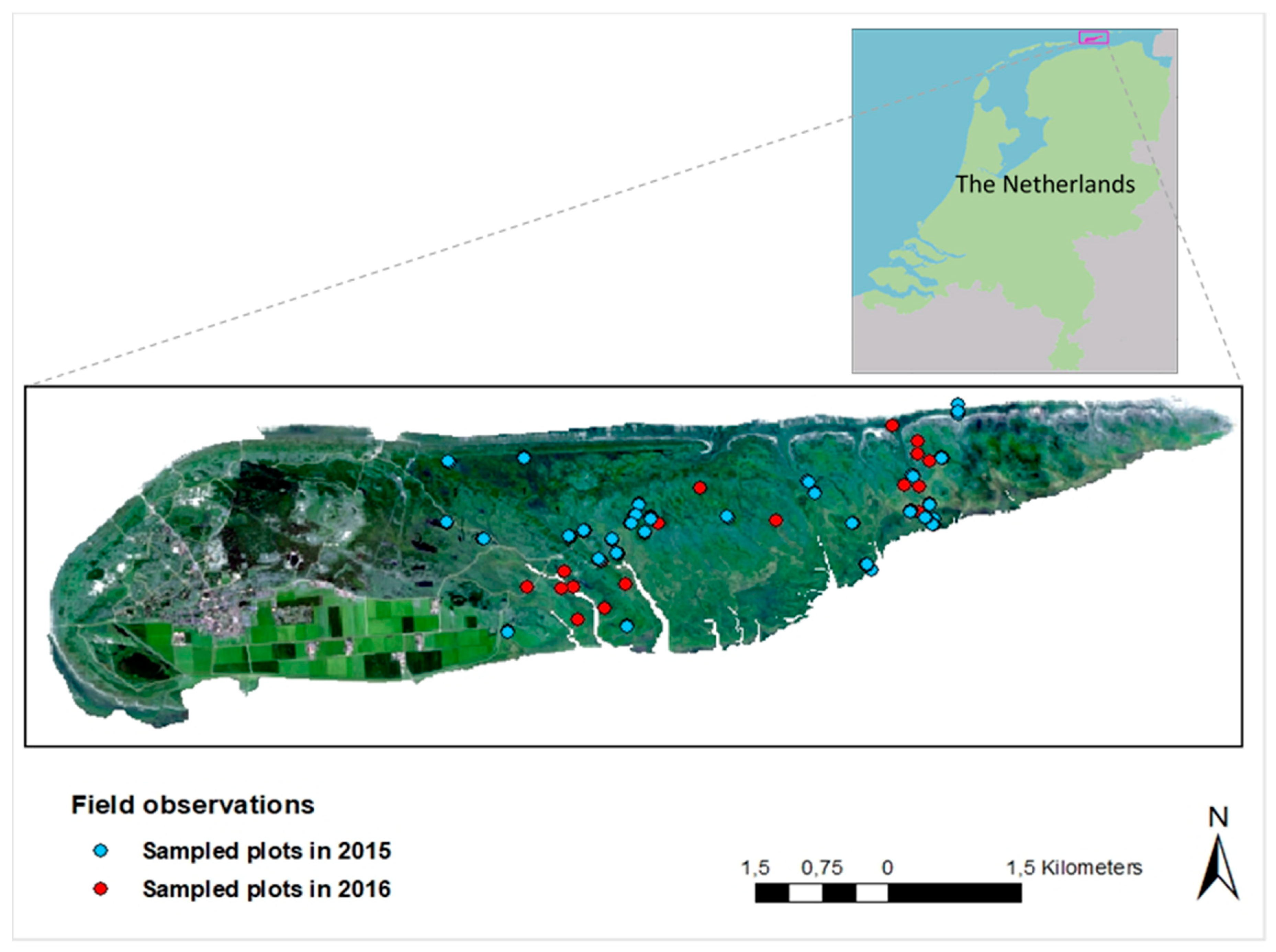
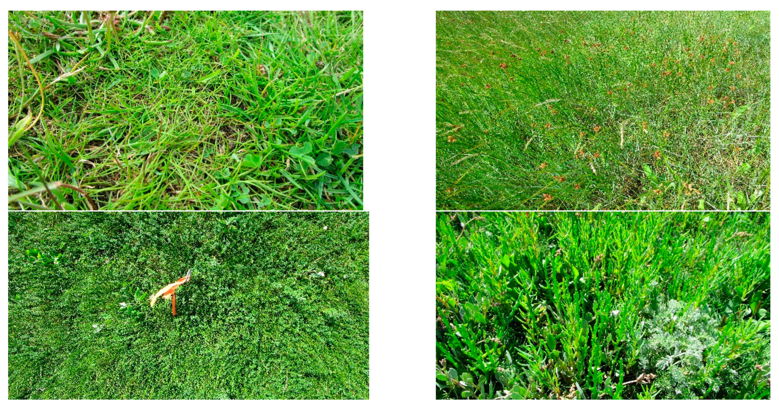
2.1. Study Area

This study was conducted in the Dutch barrier island of Schiermonnikoog, which is located between the North Sea and the Wadden Sea at approximately 53°30′ N, 6°10′ E and is about 40 km2 in size (Figure 1). The annual mean temperature of the island is 10.2 ± 0.72 °C (mean ± standard deviation (SD)) with an annual rainfall of 824 ± 149.1 mm [84]. The island’s diverse vegetation cover is linked to features such as dunes, forest, polder, salt marshes, and the mudflats as well as minor altitudinal differences that influence the frequency and duration of flooding [85]. The main vegetation cover includes different species of herbs and grasses (Figure 2), while some patches of forest and shrubs exist on the dunes [86]. The herb and grass canopies are mainly characterised with an electrophile, or circular (random leaf angles) structures where the soil has relatively uniform characteristics across different vegetation communities [82].

2.2. Field Measurements
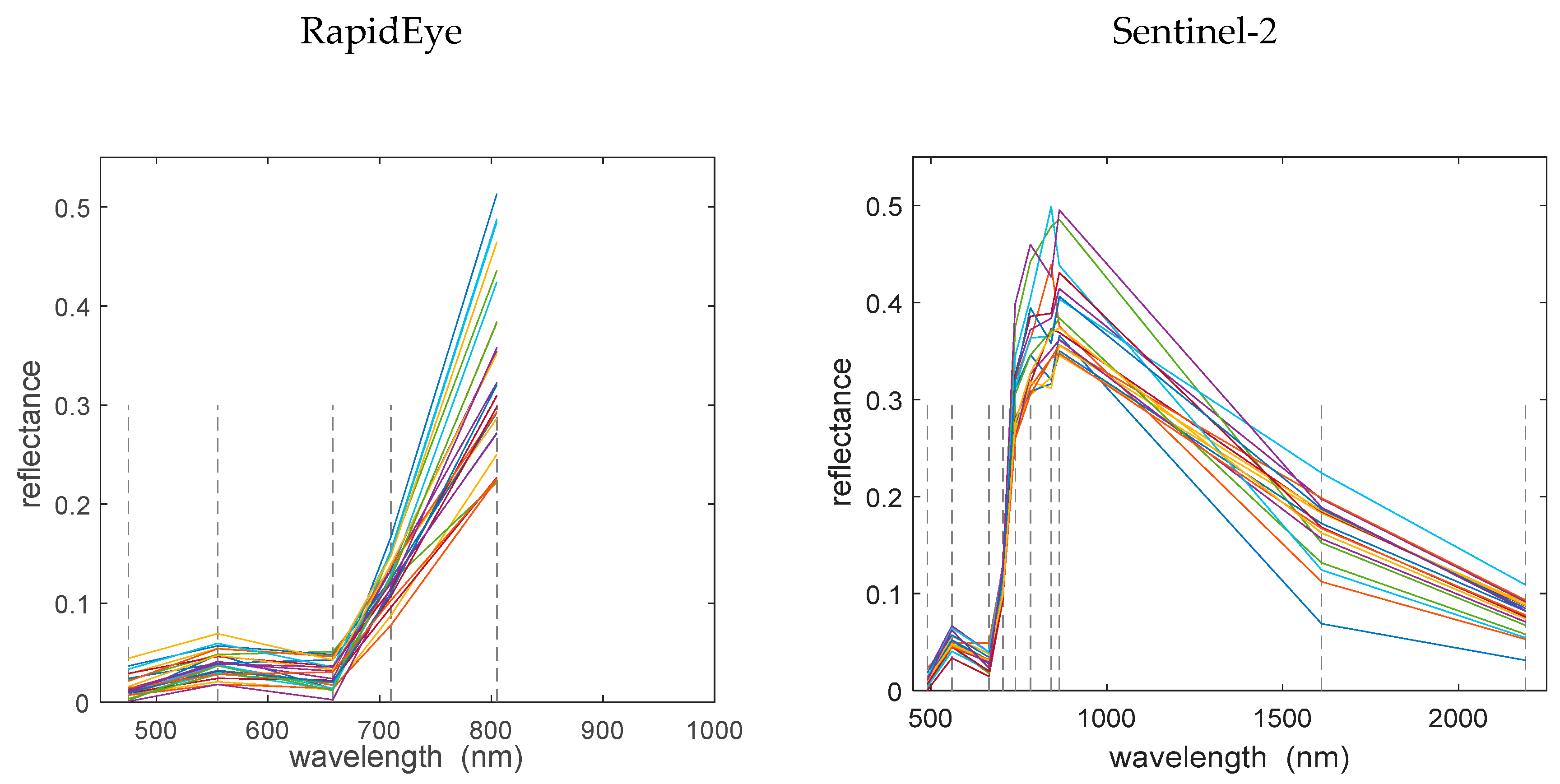
Two successive field campaigns were conducted towards the end of July 2015 (18th–25th) and July 2016 (25th–30th) to measure LAI and other plant traits. Stratified random sampling was adopted and (x,y) coordinates were randomly generated in the grassland/saltmarsh area located at the eastern part of the island. To understand the variation of LAI through the two succeeding years, the sampled plots from 2015 and those of 2016 had about one-third of overlaps. In total 50 quadratic plots (30 plots in 2015 and 20 plots in 2016) with 20 m side length were sampled (Figure 1).
In each sampling plot, several biophysical and biochemical traits were measured within five randomly selected subplots (1 × 1 m), and their averages were calculated to represent the plots. In each subplot, 30 leaves were randomly selected and the CCM-300 chlorophyll meter was used to measure the leaf chlorophyll (Cab). Next, leaf samples were collected in each subplot and stored in zipped plastic bags and transferred to the laboratory to obtain the leaf dry matter (Cm) and water content (Cw). The soil reflectance was measured from a subset of subplots using a portable spectroradiometer (ASD), USA.
LAI and average leaf angle (ALA) were non-destructively measured using a widely used optical instrument, the LAI-2200C Plant Canopy Analyzer. The instrument can be used under any daytime sky conditions [87], and makes some assumptions, such as random spatial distribution of leaves, that affect the measurements accuracy. The degree to which these assumptions are met will affect the measurements of LAI and ALA. The reader is referred to [87] for the detailed description of the instrument. In each subplot, six below and two above-canopy radiation measurements were made with the sun behind the operator and using a view restrictor of 45°. The LAI of each plot was then calculated as the average LAI measurements of its subplots.
The LAI-2200 measurements correspond to the plant area index (PAI) [27]. The PAI includes photosynthetic and non-photosynthetic components [88]. During the measurements, when non-photosynthetic components (dried leaves) were present within the plot, the LAI readings were modified considering the percentage of green (and dead) leaves which was estimated by visual inspection in each plot (LAI = (LAIreadings × fraction of green leaves)), and hereafter these measurements are referred as LAI values. Table 1 summarises the statistics of the LAI values measured in summer 2015 and 2016 in the study area.

2.3. Satellite Data

2.3.1. Sentinel-2

The Sentinel-2 Level-1C product was obtained from the Copernicus Open Access Hub (https://scihub.copernicus.eu/) concurrent to the time of the field campaign (30 July 2016). To acquire Level-2A top of canopy reflectance (TOC) data, the image was atmospherically corrected using the Sen2Cor processor. Sentinel-2 offers spectral data in 13 bands from 443 to 2190 nm with three red edge bands centred at 705 nm, 740 nm, and 783 nm, respectively. For this study, the 60 m resolution bands suitable for coastal (C, 443 nm), water vapour (WV, 1375 nm) and cirrus detection (CI, 1376) studies were not utilised. Reflectance spectra of the plots sampled in 2016 were extracted from the TOC data. The centre coordinates of the sample plots (20 × 20 m) were overlaid on the Sentinel-2 image (20 m), and the reflectance of the corresponding pixels was extracted for each sample plot (Figure 3).

2.3.2. RapidEye Data

The RapidEye satellite constellation consists of five identical small satellites and is capable of collecting a large volume of data covering over 6 million square kilometres per day [89]. The five satellites contain identical sensors and are equally calibrated and travel on the same sun-synchronous orbit at an altitude of 630 km. RapidEye offers spectral data in five bands from 440 to 850 nm with a red edge band at the central wavelength at 710 nm. We used the RapidEye image acquired for Schiermonnikoog on 18 July 2015, concurrent with the time of field campaign. The image was systematically geo-corrected and ortho-rectified at a spatial resolution of 5 m [90]. To obtain the TOC reflectance data, ATCOR-2 was used for atmospheric and topographic correction [91]. The corrected image was used to retrieve the average reflectance of each sampled plot in 2015. As the pixel size was 5 m, a pixel window of 3 by 3 (i.e., 15 × 15 m) centred around the central position of a plot was used for collecting grass reflectance for each sample plot (20 × 20 m). Figure 3 demonstrates the extracted reflectance of the sample plots in 2015 and 2016 from RapidEye and Sentinel 2 images, respectively.

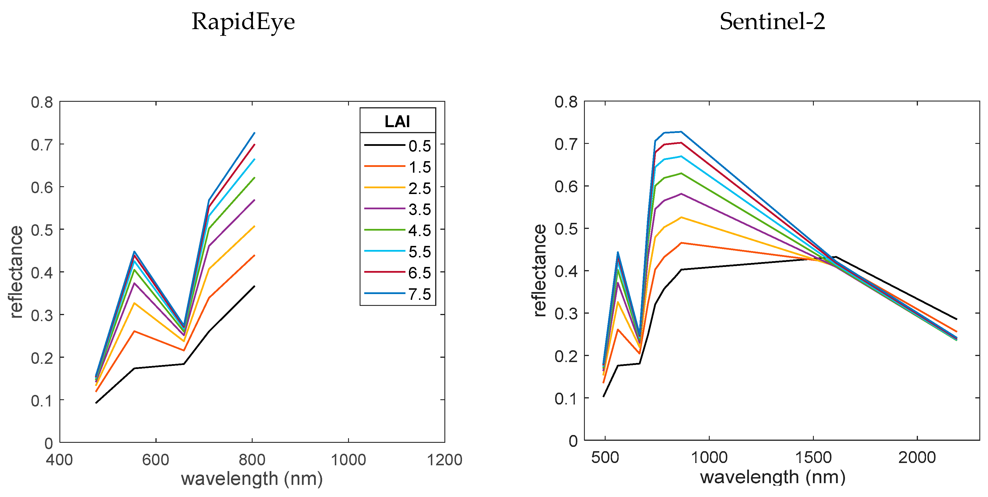
2.4. The PROSAIL Radiative Transfer Model

The widely used PROSAIL radiative transfer model [51] was selected to retrieve LAI in the wetland of Schiermonnikoog. The PROSAIL model is a compound of the SAILH canopy reflectance model [52,53,92] and the PROSPECT leaf optical properties model [25,50,93]. PROSAIL requires a limited number of input parameters, which facilitates the model inversion. It has been used for retrieval of biophysical parameters in a wide range of vegetation canopies [27,48,51,57,58,66,69,72,94,95] with various degrees of success. The overall suitability of PROSAIL for grassland studies has been demonstrated by [48,96], and the capacity of the model to simulate spectra of heterogeneous grassland in forward mode has been demonstrated in our earlier studies [27,30,95]. In the current study, we performed local sensitivity analysis [97] to understand the impact of each model input parameter, in particular, LAI, on the simulated canopy reflectance of RapidEye and Sentinel-2. We examined the effect of each model input parameter on the corresponding spectral reflectance of RapidEye and Sentinel-2 by systematically varying one parameter value at the time and keeping the rest of the parameters at their constant mean values. The model parameters that did not affect either RapidEye or Sentinel-2 simulated reflectance spectra were further fixed to constant values in the subsequent generation of LUTs.
The PROSPECT leaf model simulates the leaf hemispherical reflectance and transmittance as a function of four input parameters: the leaf chlorophyll a + b content Cab (µg cm−2); the dry matter content Cm (g cm−2); the equivalent water thickness Cw (cm) and the leaf structural parameter N (unitless). The simulated leaf reflectance and transmittance by PROSPECT are inputs into the SAILH which is a one-dimensional bidirectional turbid medium radiative transfer model and has been modified for the hot spot effect in plant canopy reflectance [92]. The SAILH model entails eight input parameters for simulation of the top-of-canopy bidirectional reflectance. These parameters are solar zenith angle, sensor viewing angle, relative azimuth angle, the fraction of diffuse incoming solar radiation, the hot spot size parameter, LAI, average leaf inclination angle, and background soil reflectance. In order to address the soil brightness variation triggered by moisture and roughness, a multiplicative soil brightness parameter was used [27,98].

2.5. Parametrization and Look-Up Table (LUT) Inversion

Look-up tables (LUT) provides a feasible approach for the inversion of RTMs [47]. LUT inversion allows performing a global search and in comparison to other inversion methods such as numerical optimisation and neural networks avoids unexpected behaviour when the canopy spectral properties are not well presented by the simulated spectra [99]. The LUT dimensions have a significant role in the retrieval accuracy of the parameters involved [27,30,100,101]. Therefore, for both 2015 and 2016 datasets used in this study, 500,000 parameter combinations were randomly generated using uniform distributions [30,57] which were then used in the forward calculation of the PROSAIL model. Furthermore, the spectral response functions of RapidEye and Sentinel-2 bands were not considered in the PROSAIL simulations.
Since reflectance data were obtained from RapidEye and Sentinel-2 imagery acquired at a known date and time, three PROSAIL input parameters related to sun and sensor geometries including sensor viewing angle (12°, 8°), relative azimuth angle (109°, 126°), and solar zenith angle (33°, 36°) were fixed based on the image specifications. Moreover, due to the minor influence of the fraction of diffuse incoming solar radiation (skyl) on canopy reflectance [102] and the lack of onsite measurements, a fixed value of 0.1 was used for this parameter [27,35,76]. The other input parameters were then generated randomly using 500,000 parameter sets to realise the LUTs for model inversion. The values of these model input parameters are described in Table 2.
We interpolated the average bare soil reflectance spectra which was measured during the field campaign to the spectral bands setting of Sentinel-2 and RapidEye to present the soil optical properties. To explain the soil roughness and moisture in the island, we also varied the range of the scale parameter [98] (Table 2). Field measurements (LAI, ALA, Cab, Cm, and Cw) were used to define the approximate range of “free” model parameters [95,103]. Limiting the parameter space has been suggested in many studies [27,48,104] and assists in regularisation of the ill-posed problem of model inversion [103]. For the hot spot size parameter, a range of 0.05 to 0.1 was selected [48,105]. Furthermore, a range of 1.5 to 1.9 was used for leaf structural parameter N [27,30], which was in agreement with the mean value (N = 1.6) used for grassland species by [96].
To find the solution to the inverse problem for given canopy reflectance spectra obtained from RapidEye and Sentinel-2 images, for each modelled reflectance spectra of the LUTs, the root means square error (RMSE) between measured (reflectance value from the Rapid-Eye or Sentinel-2) and modelled spectra (in LUT) is considered as the cost function according to:
RMSE = k = 1 n ( ρ i m a g e λ ρ L U T λ ) 2 n
where ρimage is the extracted reflectance from the Sentinel-2 or RapidEye image for the sample plots, ρLUT is the simulated reflectance from the corresponding LUT, n is the number of spectral bands, and λ is the corresponding spectral band of Sentinel-2 and RapidEye, respectively.
The set of model input parameters which corresponded to the simulated reflectance from each LUT that best matched the measured reflectance from Sentinel-2 or RapidEye with the minimum cost function (smallest RMSE) is regarded as the solution. In other words, the LAI of each plot was retrieved from the large LUTs when the measured reflectance obtained from the images had the smallest difference (RMSE) with the RTM simulated reflectance. Consequently, for each plot, the LUTs were sorted according to the cost function (RMSE) and the set of variables providing the minimum RMSE were considered as solutions (estimated LAI). However, because of the ill-posed nature of the inversion, this solution may not always be unique [106]. To address this and to improve the LAI retrieval, instead of using a single solution, the mean parameters from the best 10, 50 and 100 solutions were considered [30,103]. To increase the robustness of inversions, the proper selection of features is recommended [3]. Selection of relevant and important bands which are well modelled by RTM is known to enhance the inversion [95,107,108]. Since RapidEye data had only five spectral bands, spectral subsetting was explored only for the Sentinel-2 data. We examined whether LAI estimates from Sentinel-2 data through inversion of PROSAIL would be enhanced by selecting optimal spectral subsets. Four spectral subsets were selected considering i) the spectral bands with central wavelengths comparable to those from RapidEye, ii) NIR and SWIR spectral bands, iii) red edge spectral bands, and iv) excluding spectral bands with high average absolute errors (AAE) (specified threshold (RMSE ≤ 0.02)) between simulated and measured reflectance of Sentinel-2. More details on the calculation of AAE can be found in [27,30].

2.6. Model Validation and Mapping

The retrieval of LAI in Schiermmonikoog island through inversion of PROSAIL using Sentinel-2 and RapidEye data was validated using the measured LAI from the field campaigns. To examine the LAI accuracy, the coefficient of determination (R2), the RMSE, and the normalised RMSE (NRMSE, RMSE/range) [27] between measured and retrieved LAI were assessed. The LAI map of the island was then produced using RapidEye and Sentinel-2 images and PROSAIL inversion. The existing vegetation map of the island [109], was utilised to mask out the peripheral land covers (waterbodies, bare dunes and buildup area) from Sentinel-2 and RapidEye data. The masked images were then used as input to the inversion process, and the maps of predicted LAI were retrieved using the minimum RMSE criterion (best fitting spectra).

3. Results

3.1. Variations in Leaf Area Index (LAI) Measurements in 2015 and 2016

As can be observed from the summary statistics of the field-measured LAI (Table 1), the LAI values in 2016 had a larger range in comparison to the measured LAI data from 2015. In 2015, the mean LAI was 2.58 m2/m2 while the mean LAI for data obtained in 2016 was 3.31 m2/m2. The measured LAI from both years showed relative high variability, while the sampled LAI in 2015 demonstrated slightly higher variation (coefficient of variation = 0.42) compared to those in 2016 (coefficient of variation = 0.40). Similar trends were observed for the measured chlorophyll, where the range was smaller in 2015 compared to those from 2016. The range of other measured variables from the two years showed relatively little variation (data not shown).
The results of the sensitivity analysis of PROSAIL for LAI estimation using RapidEye and Sentinel-2 spectral band settings is presented in Figure 4. As was expected, LAI is exerting a strong influence on the simulated canopy reflectance for both sensors. Almost all RapidEye spectral bands demonstrated sensitivity to LAI variation. For Sentinel-2 also, the sensitivity of all spectral bands are underlined in the figure, although it seems that that LAI’s influence on the visible and NIR spectral bands is more pronounced. The simulated canopy reflectance of both sensors was largely affected by all other model input parameters (not shown), except for the leaf water content (Cw) which displayed no influence on the simulated canopy reflectance spectra of RapidEye and only influenced the NIR (lightly) and mostly the SWIR spectral bands of Sentinel-2. For this reason, leaf water content was fixed to a constant value (Cw = 0.01, g cm−2) for the generation of RapidEye LUT only, but not for Sentinel-2.

3.2. Inversions Based on the Minimum Root Means Square Error (RMSE) Criterion

Using each LUT, the difference (RMSE) between the simulated and measured canopy reflectance obtained from the corresponding image was calculated, and the results were sorted using the minimum RMSE criterion. The simulated reflectance from the LUT which yield the smallest RMSE with a measured reflectance (obtained from the RapidEye and Sentinel-2 images) was regarded as the best fit or best-simulated canopy reflectance. Accordingly, the set of model input parameters corresponding to the “best fit” from the LUT were regarded as the solution. Figure 5 demonstrates the canopy reflectance spectra obtained from Sentinel-2 and RapidEye data and the so-called best-fit reflectance from the LUTs calculated in this way for two plots in 2015 and two plots in 2016 with different LAI values.
As Figure 5 illustrates, the measured reflectance from RapidEye and Sentinel-2 are modelled differently using PROSAIL. For Sentinel-2, the observed mismatch between the two canopy reflectance is more noticeable for the NIR and green bands while for the RapidEye data this mismatch is more pronounced in the red band.
To examine these discrepancies between the measured and modelled spectral reflectance from RapidEye and Sentinel-2 the AAEs were considered [21]. In Figure 6, the AAEs between the reflectance from RapidEye and Sentinel-2, and their corresponding best-fit spectra (resulting in the lowest RMSE among the image and simulated canopy reflectance) from the two LUTs are shown. It shows that generally the dissimilarities between RapidEye and Sentinel-2 measured and modelled reflectance follow a similar trend. The AAEs calculated for the data from the two sensors demonstrate comparable drift in the visible region, with the green band showing the highest error in this region. While using Sentinel-2 data the infrared and the third red edge bands present relatively larger errors.
Figure 7 presents scatterplots illustrating the relationship between measured and retrieved LAI using the smallest RMSE criterion. In general, the retrieved and measured LAI had somehow reasonable relationships, while this relationship was stronger in 2016 using Sentinel-2 data. The measured and estimated LAI in 2016 had a higher coefficient of determination (R2 = 0.55) and lower error (NRMSE = 0.17) in comparison to those from RapidEye in 2015. The deviation of estimated LAI in 2015 from one to one line was more toward the higher values.

3.3. Inversion Using Various Solutions

To overcome the ill-posedness of the model inversion and to enhance the LAI retrieval, the use of multiple solutions were examined. The significance of using multiple solutions instead of a single solution corresponding to the minimum RMSE has been shown in our earlier studies [24,86]. Hence we further assessed how the use of the best 10, 50, and 100 solutions from the RapidEye and Sentinel-2 LUTs would affect the retrieval accuracy of LAI. The relationship between measured and retrieved LAI values using alternative solutions was then studied in both datasets using the R2, RMSE, and NRMSE values. The results of these analyses are demonstrated in Table 3. In general, using multiple solutions, higher retrieval accuracies were observed for all alternative solutions from Sentinel-2 data in comparison to those from RapidEye. As can be realised from the table, using the RapidEye and Sentinel-2 data and the mean of the first 10 best solutions resulted in higher R2 (0.51 and 0.59) and lower NRMSE (0.24 and 0.16), respectively compared to the use of minimum RMSE. Using the mean of the best 50 and 100 solutions in both datasets decreased the R2 values between measured and estimated LAI with almost no effect on their NRMSE values.

3.4. Inversion Using Spectral Subsets from Sentinel-2

RapidEye had only five spectral bands in which none returned a large AAE. Therefore, we only examined the effect of spectral subsets on LAI retrieval using Sentinel-2 data. The significance of using four spectral subsets was assessed using R2, RMSE, and NRMSE between the retrieved and measured LAI. As such first, the spectral bands which resulted in an AAE larger than 0.02 (see Figure 5) were selected assuming these are the bands with large errors [27]. These were the NIR (842 nm, 865 nm) and the red edge (783 nm) bands. Accordingly, the LUT of Sentinel-2 was inverted discounting these spectral bands (subset A). Next, the spectral bands form Sentinel-2 which were comparable to those from RapidEye data were considered. These spectral bands (490 nm, 560 nm, 665 nm, 705 nm, and 783 nm) were consequently used in the inversion process (subset B). Third, the combination of NIR (842 nm, 865 nm) and SWIR (1610 nm 2210 nm) spectral bands were considered and used in the LUT inversion (subset C). Finally, the three red-edge bands (705 nm, 740 nm, 783 nm) were taken and employed for the inversion of Sentinel-2′ LUT (subset D). Retaining the four subsets from Sentinel-2 spectral data decreased the LAI accuracy with respect to using all spectral bands (Table 4). However, when the NIR and SWIR spectral bands were used (subset C), LAI was estimated with moderate accuracy (R2 = 0.44, NRMSE = 0.21).

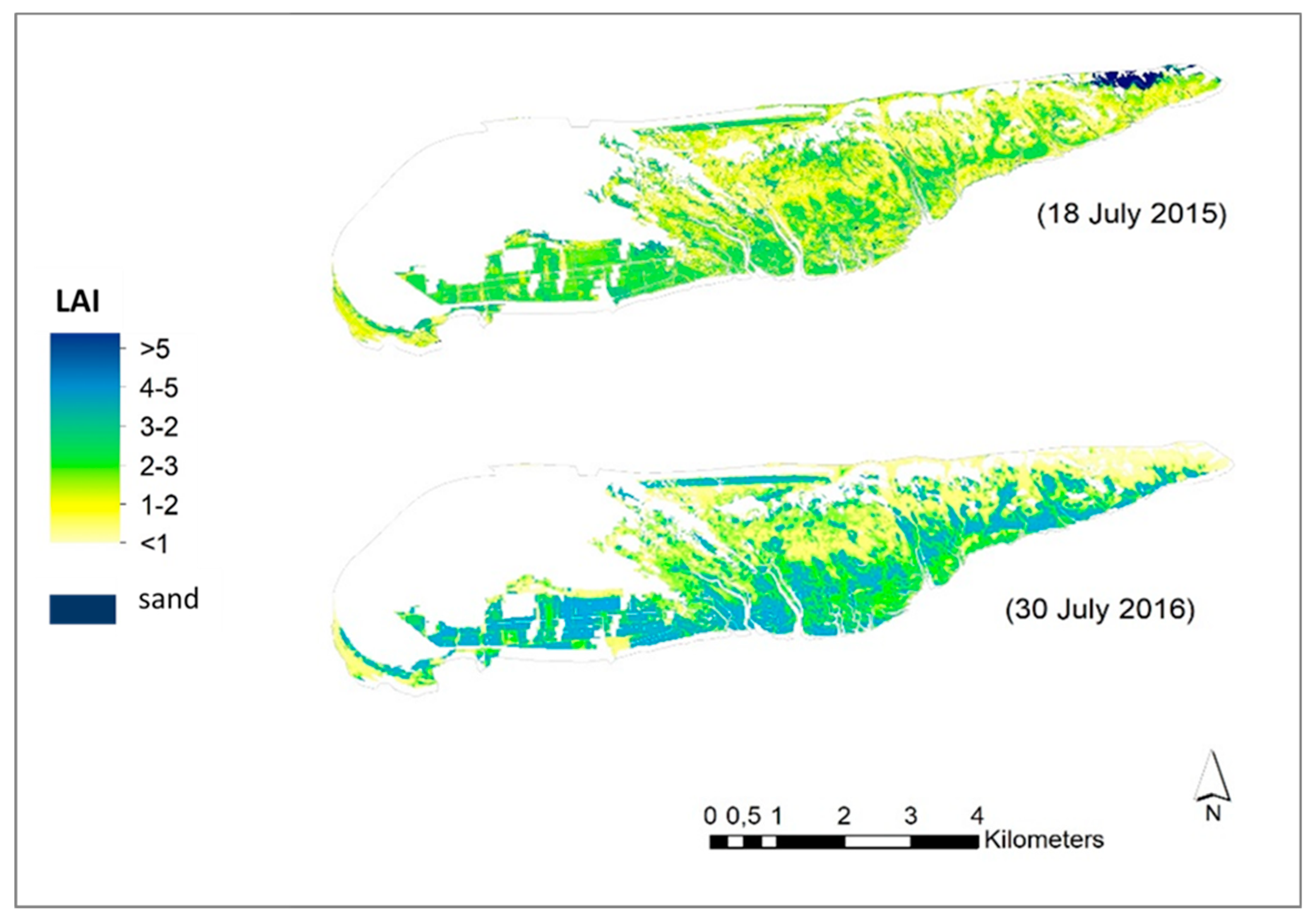
3.5. Mapping LAI for Schiermonnikoog Island

LAI was mapped for the Island using both RapidEye and Sentinel-2 data. Before producing the maps, masks were produced for saltmarshes, grass and crops using the vegetation map of the Island modified by [86] and employed to mask out the areas occupied by other land cover types (build-up area, water bodies and dunes) in the Rapid-Eye and Sentinel-2 imageries. We intentionally included the agricultural fields in the masked images since the suitability of PROSAIL in mapping LAI of crops has been earlier confirmed [71,73,78]. The masked RapidEye and Sentinel-2 images were then used as inputs for the inversion process of the two LUTs. Accordingly, the LAI maps of the island were then retrieved using the best fitting spectra. Figure 8 shows the LAI maps derived from RapidEye and Sentinel-2. Their mean and variance agreed with those observed during the field campaigns (Table 1). Although the spatial distribution of LAI from the two years are comparable, the Sentinel-2 derived map has larger range and shows higher LAI values in comparison to those from RapidEye. Nevertheless, the map produced from RapidEye data (owing to its fine spatial resolution) presents more details on the spatial variation of LAI.

4. Discussion

In this study, the feasibility of retrieving LAI of saltmarsh vegetation using PROSAIL and high spatial resolution RapidEye and Sentinel-2 satellite images was demonstrated. Using the minimum RMSE criterion, we observed a good relationship between the field measured and estimated LAI values using the RapidEye (R2 =0.50, RMSE = 1.27 m2/m2 and NRMSE = 0.27) and Sentinel-2 data (R2 = 0.55, RMSE = 0.87 m2/m2 and NRMSE = 0.17) (Figure 7). Furthermore, the errors obtained decreased when multiple solutions were utilised from both LUTs (Table 3). The measured LAI from the field campaigns showed moderate variability (coefficient of variation= 0.42 and 0.40 for 2015 and 2016, respectively), hence moderate retrieval accuracies [110] were obtained for both years. Furthermore, the sensible retrieval accuracies of LAI which were obtained using data from the two sensors can also be explained by the large sizes of the two LUTs (500,000 records) that permitted appropriate sample selection. The significance of appropriate sample selection in the LUT approach is highlighted for model optimisation and efficiency as well as for the proper understanding of the ecosystem conditions [101].
In vegetation canopies, biophysical variables (such as LAI) play a significant role in characterising the canopy reflectance [24,111]. However, the relationships between these variables and canopy reflectance are complex, as the reflectance of the canopy is a function of leaf optical properties, canopy architecture, background soil as well as illumination and viewing geometry [24,108,112,113]. PROSAIL has been successful in explaining these interactions mainly in nonwoody vegetation and for modelling LAI in various vegetation types [51]. Few studies have demonstrated the suitability of the model for Mediterranean grassland ecosystems utilising hyperspectral measurements [27,30,48,95,96]. Also recently the PROSAIL model and airborne hyperspectral data have been successfully used in the wetland for retrieval of leaf mass area [32]. However, results of the current study confirmed that the PROSAIL model could be used in combination with data from new multispectral sensors such a Sentinel-2 and RapidEye to study the biophysical properties of grasslands in a saltmarsh ecosystem.
It is known that LAI plays a key role in the magnitude of canopy reflectance [31]. Likewise, the results of sensitivity analysis confirmed that the canopy spectral reflectance from both RapidEye and Sentinel-2 sensors were highly sensitive to LAI variations (Figure 4). In general, the variation of all PROSAIL input parameters influenced the simulated RapidEye (475–805 nm) and Sentinel-2 (490–2190 nm) reflectance except leaf water content (not shown). Therefore, prior knowledge from field observations of input parameters assisted in model parameterisation. The leaf water content did not show any influence on the RapidEye simulated reflectance. This was expected as water-sensitive features mainly exist within the NIR and SWIR spectral regions [111] which are absent in RapidEye spectral data.
A relatively close match was observed between the measured and simulated reflectance of RapidEye and Sentinel-2 (Figure 5), particularly for the visible, red-edge and SWIR spectral bands (from Sentinel-2) where the AAEs were lower than 0.02 (Figure 6). Nevertheless, a spectral mismatch between the measured and simulated reflectance was noticeable at NIR spectral bands which are sensitive to LAI, nitrogen content, leaf structure and dry matter [10,11,30,48]. These results are in agreement with earlier findings by [11,30,48] who observed that the spectral bands in the NIR spectral region (around 800–850 nm) demonstrate relatively high errors using hyperspectral data. It is anticipated that the spectral bands from this region (800–850 nm) are prominently sensitive to noise or are not well modelled by RTM.
The relationship between the field measured and retrieved LAI using the smallest RMSE criterion was stronger employing the Sentinel-2 data (NRMSE = 0.17, RMSE = 0.87 m2/m2, R2 = 0.55) in comparison of using the RapidEye data (NRMSE = 0.27, RMSE = 1.27 m2/m2 and R2 = 0.50). These accuracies are lower than those obtained by [48,95] who utilised hyperspectral data and the PROSAIL model with a LUT-based inversion for LAI estimation in grasslands (RMSE = 0.63 m2/m2, 0.53 m2/m2 and R2 = 0.89, 0.91). The coefficient of determinations obtained in this study are also lower than those in our earlier studies where we used hyperspectral data in Mediterranean grassland to retrieve LAI from PROSAIL inversion (R2 = 0.86) albeit with a higher RMSE (RMSE = 0.89 m2/m2) [27,30]. The obtained errors from Sentinel-2 data are, however, comparable to those from [96] who used various hyperspectral measurements for LAI estimation in central Europe (RMSE = 0.86 m2/m2, 0.74 m2/m2). Sentinel-2 data benefits from spectral bands at NIR and SWIR regions which are crucial for LAI studies [31,44]. Therefore, the lower retrieval accuracy obtained using the RapidEye data partly is explained by the absence of these spectral bands. Nevertheless, RapidEye data has a very fine spatial resolution which makes the sensor unique and less prone to mixed pixels challenges. This importance was confirmed when spectral subset B of Sentinel 2 with central wavelengths similar to those from RapidEye were selected (490 nm, 560 nm, 665 nm, 705 nm, and 783 nm) for the inversion and returned very low retrieval accuracy for LAI in comparison to those from RapidEye (Table 4).
To address and reduce the ill-posedness of model inversion some approaches are investigated in the literature such as choosing a proper spectral subset [30,101], ecological constraints [11,114], prior knowledge [100,106] and spatial regularisation [75,115]. In this study, the prior field information which was acquired during the two field campaigns were used to determine the range of model input parameters and to limit the implausible combinations. Moreover, the LAI was estimated using the mean of the first 10, 50 and 100 best solutions from the LUTs. The result of this analysis demonstrated that utilising the mean of the first 10 best solutions the retrieval accuracy of LAI would increase from both RapidEye and Sentinel-2 data (R2 = 0.51, 0.59 NRMSE = 0.24, 0.16, respectively) (Table 3). The obtained results are in agreement with that of [30,48,63] who demonstrated that the use of multiple solutions results in more robust retrieval accuracy.
In general, biophysical variables such as LAI, canopy architecture (e.g., leaf angle distribution) and biomass present major contributions to the canopy reflectance, mainly in near-infrared (NIR) and SWIR regions [10,29,31,35,44,116]. This was confirmed in our study when NIR and SWIR spectral bands of Sentinel-2 were used as a spectral subset for the inversion (Table 4). Utilising different Sentinel-2′ spectral subsets showed that the spectral subset C which contained the four spectral bands of NIR and SWIR (842 nm, 865 nm, 1610 nm, 2210 nm), in comparison to using other spectral subsets resulted in higher retrieval accuracy for LAI (R2 = 0.44, NRMSE = 0.21). As such, [73] examined the LAI retrieval of crops using simulated Sentinel-2 data as well as various parametric and non-parametric models and found that SWIR bands (1610 nm, 2210 nm) in combination with the green band (490 nm) are important spectral bands for LAI estimation. Furthermore, [78] demonstrated that the red (665 nm) and NIR (842 nm) spectral bands of Sentinel-2 are important bands for LAI prediction of the potato crop. The practice of the other three spectral subsets from Sentinel-2 data did not improve the retrieval accuracy signifying the properly located spectral bands from the sensor.
For the generation of the LAI maps, the smallest RMSE criterion was used in the inversion of RapidEye and Sentinel-2 LUTs. Overall, the LAI maps obtained from both sensors presented the variation of LAI in the island well. Although the spatial variation of LAI from the two maps were somehow comparable, higher LAI values were observed in the derived Sentinel-2 map of 2016 which was in agreement with the larger range of measured LAI in 2016. As was expected, the map produced from RapidEye data, due to its higher spatial resolution of 5 m, presented a detailed overview of the variation of LAI. Nevertheless, a concise study of the maps revealed that due to absence of SWIR spectral bands in RapidEye sensor, part of the island in 2015 (in the northeast) which was dominated by sand rather than vegetation cover (low reflectance in red and very high reflectance in NIR) was identified as region with very high LAI values (LAI > 7). In the presented maps, this area is identified in the 2015 map as the sand class. Our findings emphasise the importance of multi-spectral satellite sensors such as Sentinel-2 with spectral bands at NIR and SWIR regions for regional mapping of vegetation LAI in wetland ecosystems using radiative transfer models. Monitoring vegetation status and tracking EBVs such as LAI in these systems is vital for their sustainability and proper use and promote the Ramsar Convention’s common agenda to halt loss of biodiversity.

5. Conclusions

The results obtained in this study revealed the feasibility of the two broadband multispectral (Sentinel-2 and RapidEye) sensors for retrieval of LAI in the saltmarsh of Schiermonnikoog via the inversion of PROSAIL. In general, LAI estimated from Sentinel-2 data had higher accuracy in comparison to those from RapidEye. Although Rapid Eye had a finer spatial resolution than Sentinel-2, the enhanced spectral range and resolution offered by Sentinel-2, e.g., three red edge bands, trumped the benefit of higher spatial resolution offered by Rapid Eye which in comparison had only one red edge band. The highest retrieval accuracies were obtained using all spectral bands of RapidEye and Sentinel-2 and the mean of the best ten solutions. When spectral subsetting of Sentinel-2 was considered, the spectral subset which contained four spectral bands of NIR and SWIR resulted in higher LAI retrieval accuracy in comparison to other spectral subsets studied and emphasised the importance of Sentinel-2 data for LAI studies. Our results highlight the suitability of PROSAIL when coupled with broadband satellite data for regional and global mapping of LAI in saltmarsh/grassland ecosystems.
The LAI retrieval accuracy through model inversion is not only affected by uncertainties in satellite reflectance data and the RTM inadequacies [2] but also by, uncertainties related to LAI in situ measurements. In our study, LAI was measured using LAI-2200 instrument which accounts for the existence of both green and dead leaves. Although in this study we accounted for the percentage of non-photosynthetic components (dried leaves) of the measured LAI, no corrections for clumping effects or non-random distribution of leaves were considered. Further improvement of retrieval accuracy is expected when clumping effects or destructive sampling for LAI measurements are considered.

Author Contributions

R.D. Conceptualized the paper and performed the experiment, analyzed the data, and wrote the manuscript. All the coauthors helped in editing the draft as well as providing critical comments. A.S. was also the project investigator. T.W. and T.W.G. participated in the field campaigns and assisted in field measurements.

Funding

This study was partially funded by the European Space Agency’s Innovators-III project “Remote Sensing for Essential Biodiversity Variables” (ESRIN Contract No. 4000113386).

Acknowledgements

We acknowledge support from Henk Kloosterman during the field data collection in 2015. We thank Willem Nieuwenhuis for his assistance with the image preprocessing.

Conflicts of Interest

The authors have no conflict of interest associated with this publication.

References

  1. Jonckheere, I.; Fleck, S.; Nackaerts, K.; Muys, B.; Coppin, P.; Weiss, M.; Baret, F. Review of methods for in situ leaf area index determination: Part I. Theories, sensors and hemispherical photography. Agric. For. Meteorol. 2004, 121, 19–35. [Google Scholar] [CrossRef]
  2. García-Haro, F.J.; Campos-Taberner, M.; Muñoz-Marí, J.; Laparra, V.; Camacho, F.; Sánchez-Zapero, J.; Camps-Valls, G. Derivation of global vegetation biophysical parameters from EUMETSAT Polar System. ISPRS J. Photogramm. Remote Sens. 2018, 139, 57–74. [Google Scholar] [CrossRef]
  3. Baret, F.; Buis, S. Estimating canopy characteristics from remote sensing observations: Review of methods and associated problems. In Advances in Land Remote Sensing System, Modeling, Inversion and Application; Liang, S., Ed.; Springer: Berlin, German, 2008; pp. 173–201. [Google Scholar]
  4. GCOS. Systematic Observation Requirements for Satellite-Based Data Products for Climate. Supplemental Details to the Satellite-Based Component of the “Implementation Plan for the Global Observing System for Climate in Support of the UNFCCC (2010 Update)”; GCOS: Geneva, Swithzerland, 2011. [Google Scholar]
  5. Pettorelli, N.; Wegmann, M.; Skidmore, A.; Mücher, S.; Dawson, T.P.; Fernandez, M.; Lucas, R.; Schaepman, M.E.; Wang, T.; O’Connor, B.; et al. Framing the concept of satellite remote sensing essential biodiversity variables: Challenges and future directions. Remote Sens. Ecol. Conserv. 2016, 2, 122–131. [Google Scholar] [CrossRef]
  6. Skidmore, A.K.; Pettorelli, N.; Coops, N.C.; Geller, G.N.; Hansen, M.; Lucas, R.; Mücher, C.A.; O’Connor, B.; Paganini, M.; Pereira, H.M.; et al. Environmental science: Agree on biodiversity metrics to track from space. Nature 2015, 523, 403–405. [Google Scholar] [CrossRef] [PubMed] [Green Version]
  7. Zhou, X.; Zhu, Q.; Tang, S.; Chen, X.; Wu, M. Interception of PAR and relationship between FPAR and LAI in summer maize canopy. In Proceedings of the IEEE International Geoscience and Remote Sensing Symposium, Toronto, ON, Canada, 24–28 June 2002; Volume 6, pp. 3252–3254. [Google Scholar]
  8. Pierce, L.; Running, S.W.; Walker, J. Regional-scale relationships of leaf area index to specific leaf area and leaf nitrogen content. Ecol. Appl. 1994, 4, 313–321. [Google Scholar] [CrossRef]
  9. Petcu, E.; Petcu, G.; Lazar, C.; Vintila, R. Relationship between leaf area index, biomass and winter wheat yield obtained at Fundulea, under conditions of 2001 year. Rom. Agric. Res. 2003, 19, 21–24. [Google Scholar]
  10. Ali, A.M.; Darvishzadeh, R.; Skidmore, A.K.; van Duren, I. Effects of Canopy Structural Variables on Retrieval of Leaf Dry Matter Content and Specific Leaf Area from Remotely Sensed Data. IEEE J. Sel. Top. Appl. Earth Obs. Remote Sens. 2016, 9, 898–909. [Google Scholar] [CrossRef]
  11. Wang, Z.; Skidmore, A.K.; Darvishzadeh, R.; Wang, T. Mapping forest canopy nitrogen content by inversion of coupled leaf-canopy radiative transfer models from airborne hyperspectral imagery. Agric. For. Meteorol. 2018, 253, 247–260. [Google Scholar] [CrossRef]
  12. Schlerf, M.; Atzberger, C. Inversion of a forest reflectance model to estimate structural canopy variables from hyperspectral remote sensing data. Remote Sens. Environ. 2006, 100, 281–294. [Google Scholar] [CrossRef]
  13. Naesset, E.; Bollandsas, O.M.; Gobakken, T. Comparing regression methods in estimation of biophysical properties of forest stands from two different inventories using laser scanner data. Remote Sens. Environ. 2005, 94, 541–553. [Google Scholar] [CrossRef]
  14. Hall, F.G.; Shimabukuro, Y.E.; Huemmrich, K.F.; Applications, S.E.; Nov, N. Remote Sensing of Forest Biophysical Structure Using Mixture Decomposition and Geometric Reflectance Models. Ecol. Appl. 2011, 5, 993–1013. [Google Scholar] [CrossRef]
  15. Lefsky, M.A.; Cohen, W.B.; Acker, S.A.; Parker, G.G.; Spies, T.A.; Harding, D. Lidar Remote Sensing of the Canopy Structure and Biophysical Properties of Douglas-Fir Western Hemlock Forests. Remote Sens. Environ. 1999, 70, 339–361. [Google Scholar] [CrossRef]
  16. Huesca, M.; García, M.; Roth, K.L.; Casas, A.; Ustin, S.L. Canopy structural attributes derived from AVIRIS imaging spectroscopy data in a mixed broadleaf/conifer forest. Remote Sens. Environ. 2016, 182, 208–226. [Google Scholar] [CrossRef]
  17. Breda, N.J.J. Ground-based measurements of leaf area index: A review of methods, instruments and current controversies. J. Exp. Bot. 2003, 54, 2403–2417. [Google Scholar] [CrossRef]
  18. Weiss, M.; Baret, F.; Smith, G.J.; Jonckheere, I.; Coppin, P. Review of methods for in situ leaf area index (LAI) determination: Part II. Estimation of LAI, errors and sampling. Agric. For. Meteorol. 2004, 121, 37–53. [Google Scholar] [CrossRef]
  19. Yang, F.; Sun, J.; Fang, H.; Yao, Z.; Zhang, J.; Zhu, Y.; Song, K.; Wang, Z.; Hu, M. Comparison of different methods for corn LAI estimation over northeastern China. Int. J. Appl. Earth Obs. Geoinf. 2012, 18, 462–471. [Google Scholar]
  20. Fang, H.; Ye, Y.; Liu, W.; Wei, S.; Ma, L. Continuous estimation of canopy leaf area index (LAI) and clumping index over broadleaf crop fields: An investigation of the PASTIS-57 instrument and smartphone applications. Agric. For. Meteorol. 2018, 253–254, 48–61. [Google Scholar] [CrossRef]
  21. Francone, C.; Pagani, V.; Foi, M.; Cappelli, G.; Confalonieri, R. Comparison of leaf area index estimates by ceptometer and PocketLAI smart app in canopies with different structures. Field Crops Res. 2014, 155, 38–41. [Google Scholar] [CrossRef]
  22. Qu, Y.; Meng, J.; Wan, H.; Li, Y. Preliminary study on integrated wireless smart terminals for leaf area index measurement. Comput. Electron. Agric. 2016, 129, 56–65. [Google Scholar] [CrossRef]
  23. Darvishzadeh, R.; Skidmore, A.; Abdullah, H.; Cherenet, E.; Ali, A.; Wang, T.; Nieuwenhuis, W.; Heurich, M.; Vrieling, A.; O’Connor, B.; et al. Mapping leaf chlorophyll content from Sentinel-2 and RapidEye data in spruce stands using the invertible forest reflectance model. Int. J. Appl. Earth Obs. Geoinf. 2019, 79, 58–70. [Google Scholar] [CrossRef]
  24. Asner, G.P. Biophysical and Biochemical Sources of Variability in Canopy Reflectance. Remote Sens. Environ. 1998, 64, 234–253. [Google Scholar] [CrossRef]
  25. Jacquemoud, S.; Ustin, S.L.; Verdebout, J.; Schmuck, G.; Andreoli, G.; Hosgood, B. Estimating leaf biochemistry using the PROSPECT leaf optical properties model. Remote Sens. Environ. 1996, 56, 194–202. [Google Scholar] [CrossRef]
  26. Yoder, B.J.; Pettigrew-Crosby, R.E. Predicting nitrogen and chlorophyll content and concentration from reflectance spectra (400–2500 nm) at leaf and canopy scales. Remote Sens. Environ. 1995, 53, 199–211. [Google Scholar] [CrossRef]
  27. Darvishzadeh, R.; Skidmore, A.; Schlerf, M.; Atzberger, C. Inversion of a radiative transfer model for estimating vegetation LAI and chlorophyll in a heterogeneous grassland. Remote Sens. Environ. 2008, 112, 2592–2604. [Google Scholar] [CrossRef]
  28. Gitelson, A.A.; Vina, A.; Arkebauer, T.J.; Rundquist, D.C.; Keydan, G.; Leavitt, B. Remote estimation of leaf area index and green leaf biomass in maize canopies. Geophys. Res. Lett. 2003, 30, 52–54. [Google Scholar] [CrossRef]
  29. Houborg, R.; Anderson, M.; Daughtry, C. Utility of an image-based canopy reflectance modeling tool for remote estimation of LAI and leaf chlorophyll content at the field scale. Remote Sens. Environ. 2009, 113, 259–274. [Google Scholar] [CrossRef]
  30. Darvishzadeh, R.; Atzberger, C.; Skidmore, A.; Schlerf, M. Mapping grassland leaf area index with airborne hyperspectral imagery: A comparison study of statistical approaches and inversion of radiative transfer models. ISPRS J. Photogramm. Remote Sens. 2011, 66, 894–906. [Google Scholar] [CrossRef]
  31. Darvishzadeh, R.; Atzberger, C.; Skidmore, A.K.; Abkar, A.A. Leaf Area Index derivation from hyperspectral vegetation indicesand the red edge position. Int. J. Remote Sens. 2009, 30, 6199–6218. [Google Scholar] [CrossRef]
  32. Feilhauer, H.; Schmid, T.; Faude, U.; Sánchez-Carrillo, S.; Cirujano, S. Are remotely sensed traits suitable for ecological analysis? A case study of long-term drought effects on leaf mass per area of wetland vegetation. Ecol. Indic. 2018, 88, 232–240. [Google Scholar] [CrossRef]
  33. Ren, H.; Zhou, G. Estimating aboveground green biomass in desert steppe using band depth indices. Biosyst. Eng. 2014, 127, 67–78. [Google Scholar] [CrossRef]
  34. Mutanga, O.; Skidmore, A.K. Red edge shift and biochemical content in grass canopies. ISPRS J. Photogramm. Remote Sens. 2007, 62, 34–42. [Google Scholar] [CrossRef]
  35. Cho, M.A.; Skidmore, A.K.; Atzberger, C.G. Towards red-edge positions less sensitive to canopy biophysical parameters for leaf chlorophyll estimation using properties optique spectrales des feuilles PROSPECT and scattering by arbitrarily inclined leaves SAILH simulated data. Int. J. Remote Sens. 2008, 29, 2241–2255. [Google Scholar] [CrossRef]
  36. Gupta, R.K.; Vijayan, D.; Prasad, T.S. Comparative analysis of red-edge hyperspectral indices. Adv. Sp. Res. 2003, 32, 2217–2222. [Google Scholar] [CrossRef]
  37. Clevers, J.G.P.W.; Kooistra, L. Using hyperspectral remote sensing data for retrieving canopy chlorophyll and nitrogen content. IEEE J. Sel. Top. Appl. Earth Obs. Remote Sens. 2012, 5, 574–583. [Google Scholar] [CrossRef]
  38. Danson, F.M.; Plummer, S.E. Red edge response to forest leaf area index. Int. J. Remote Sens. 1995, 16, 183–188. [Google Scholar] [CrossRef]
  39. Hansen, P.M.; Schjoerring, J.K. Reflectance measurement of canopy biomass and nitrogen status in wheat crops using normalized difference vegetation indices and partial least squares regression. Remote Sens. Environ. 2003, 86, 542–553. [Google Scholar] [CrossRef]
  40. Clevers, J.G.P.W. Imaging spectrometry in agriculture- plant vitality and yield indicators. In Imaging Spectrometry—A Tool for Environmental Observations; Hill, J., Megier, J., Eds.; Kluwer Academic: Dordrecht, The Netherlands, 1994; pp. 193–219. [Google Scholar]
  41. Broge, N.H.; Leblanc, E. Comparing prediction power and stability of broadband and hyperspectral vegetation indices for estimation of green leaf area index and canopy chlorophyll density. Remote Sens. Environ. 2001, 76, 156–172. [Google Scholar] [CrossRef]
  42. Blackburn, G.A. Remote sensing of forest pigments using airborne imaging spectrometer and LIDAR imagery. Remote Sens. Environ. 2002, 82, 311–321. [Google Scholar] [CrossRef]
  43. Imanishi, J.; Sugimoto, K.; Morimoto, Y. Detecting drought status and LAI of two Quercus species canopies using derivative spectra. Comput. Electron. Agric. 2004, 43, 109–129. [Google Scholar] [CrossRef]
  44. Darvishzadeh, R.; Skidmore, A.; Atzberger, C.; van Wieren, S. Estimation of vegetation LAI from hyperspectral reflectance data: Effects of soil type and plant architecture. Int. J. Appl. Earth Obs. Geoinf. 2008, 10, 358–373. [Google Scholar] [CrossRef]
  45. Verrelst, J.; Camps-Valls, G.; Muñoz-Mari, J.; Rivera, J.P.; Veroustraete, F.; Clevers, J.G.P.W.; Moreno, J. Optical remote sensing and the retrieval of terrestrial vegetation bio-geophysical properties-A review. ISPRS J. Photogramm. Remote Sens. 2015, 108, 273–290. [Google Scholar] [CrossRef]
  46. Kimes, D.S.; Knyazikhin, Y.; Privette, J.L.; Abuelgasim, A.A.; Gao, F. Inversion methods for physically-based models. Remote Sens. Rev. 2000, 18, 381–439. [Google Scholar] [CrossRef]
  47. Knyazikhin, Y.; Martonchik, J.V.; Myneni, R.B.; Diner, D.J.; Running, S.W. Synergistic algorithm for estimating vegetation canopy leaf area index and fraction of absorbed photosynthetically active radiation from MODIS and MISR data. J. Geophys. Res. D Atmos. 1998, 103, 32257–32275. [Google Scholar] [CrossRef] [Green Version]
  48. Atzberger, C.; Darvishzadeh, R.; Immitzer, M.; Schlerf, M.; Skidmore, A.; le Maire, G. Comparative analysis of different retrieval methods for mapping grassland leaf area index using airborne imaging spectroscopy. Int. J. Appl. Earth Obs. Geoinf. 2015, 43, 19–31. [Google Scholar] [CrossRef] [Green Version]
  49. Schlerf, M.; Atzberger, C. Vegetation Structure Retrieval in Beech and Spruce Forests Using Spectrodirectional Satellite Data. IEEE J. Sel. Top. Appl. Earth Obs. Remote Sens. 2012, 5, 8–17. [Google Scholar] [CrossRef]
  50. Jacquemoud, S.; Baret, F. PROSPECT: A model of leaf optical properties spectra. Remote Sens. Environ. 1990, 34, 75–91. [Google Scholar] [CrossRef]
  51. Jacquemoud, S.; Verhoef, W.; Baret, F.; Bacour, C.; Zarco-Tejada, P.J.; Asner, G.P.; François, C.; Ustin, S.L. PROSPECT+SAIL models: A review of use for vegetation characterization. Remote Sens. Environ. 2009, 113, S56–S66. [Google Scholar] [CrossRef]
  52. Verhoef, W. Light scattering by leaf layers with application to canopy reflectance modeling: The SAIL model. Remote Sens. Environ. 1984, 16, 125–141. [Google Scholar] [CrossRef] [Green Version]
  53. Verhoef, W. Earth observation modeling based on layer scattering matrices. Remote Sens. Environ. 1985, 17, 165–178. [Google Scholar] [CrossRef] [Green Version]
  54. Berger, K.; Atzberger, C.; Danner, M.; D’Urso, G.; Mauser, W.; Vuolo, F.; Hank, T.; Berger, K.; Atzberger, C.; Danner, M.; et al. Evaluation of the PROSAIL Model Capabilities for Future Hyperspectral Model Environments: A Review Study. Remote Sens. 2018, 10, 85. [Google Scholar] [CrossRef]
  55. Liang, L.; Di, L.; Zhang, L.; Deng, M.; Qin, Z.; Zhao, S.; Lin, H. Estimation of crop LAI using hyperspectral vegetation indices and a hybrid inversion method. Remote Sens. Environ. 2015, 165, 123–134. [Google Scholar] [CrossRef]
  56. Duan, S.B.; Li, Z.L.; Wu, H.; Tang, B.H.; Ma, L.; Zhao, E.; Li, C. Inversion of the PROSAIL model to estimate leaf area index of maize, potato, and sunflower fields from unmanned aerial vehicle hyperspectral data. Int. J. Appl. Earth Obs. Geoinf. 2014, 26, 12–20. [Google Scholar] [CrossRef]
  57. le Maire, G.; François, C.; Soudani, K.; Berveiller, D.; Pontailler, J.-Y.; Bréda, N.; Genet, H.; Davi, H.; Dufrêne, E. Calibration and validation of hyperspectral indices for the estimation of broadleaved forest leaf chlorophyll content, leaf mass per area, leaf area index and leaf canopy biomass. Remote Sens. Environ. 2008, 112, 3846–3864. [Google Scholar] [CrossRef]
  58. Locherer, M.; Hank, T.; Danner, M.; Mauser, W. Retrieval of seasonal leaf area index from simulated EnMAP data through optimized LUT-based inversion of the PROSAIL model. Remote Sens. 2015, 7, 10321–10346. [Google Scholar] [CrossRef]
  59. Casa, R.; Jones, H.G. Retrieval of crop canopy properties: A comparison between model inversion from hyperspectral data and image classification. Int. J. Remote Sens. 2004, 25, 1119–1130. [Google Scholar] [CrossRef]
  60. Yu, F.H.; Xu, T.Y.; Du, W.; Ma, H.; Zhang, G.S.; Chen, C.L. Radiative transfer models (RTMs) for field phenotyping inversion of rice based on UAV hyperspectral remote sensing. Int. J. Agric. Biol. Eng. 2017, 10, 150–157. [Google Scholar]
  61. Casas, A.; Riaño, D.; Ustin, S.L.; Dennison, P.; Salas, J. Estimation of water-related biochemical and biophysical vegetation properties using multitemporal airborne hyperspectral data and its comparison to MODIS spectral response. Remote Sens. Environ. 2014, 148, 28–41. [Google Scholar] [CrossRef]
  62. Kattenborn, T.; Fassnacht, F.E.; Pierce, S.; Lopatin, J.; Grime, J.P.; Schmidtlein, S. Linking plant strategies and plant traits derived by radiative transfer modelling. J. Veg. Sci. 2017, 28, 717–727. [Google Scholar] [CrossRef]
  63. Darvishzadeh, R.; Matkan, A.A.A.A.; Dashti Ahangar, A. Inversion of a radiative transfer model for estimation of rice canopy chlorophyll content using a lookup-table approach. IEEE J. Sel. Top. Appl. Earth Obs. Remote Sens. 2012, 5, 1222–1230. [Google Scholar] [CrossRef]
  64. González-Sanpedro, M.C.; Le Toan, T.; Moreno, J.; Kergoat, L.; Rubio, E. Seasonal variations of leaf area index of agricultural fields retrieved from Landsat data. Remote Sens. Environ. 2008, 112, 810–824. [Google Scholar] [CrossRef]
  65. Campos-Taberner, M.; Javier García-Haro, F.; Busetto, L.; Ranghetti, L.; Martínez, B.; Amparo Gilabert, M.; Camps-Valls, G.; Camacho, F.; Boschetti, M. A Critical Comparison of Remote Sensing Leaf Area Index Estimates over Rice-Cultivated Areas: From Sentinel-2 and Landsat-7/8 to MODIS, GEOV1 and EUMETSAT Polar System. Remote Sens. 2018, 10, 763. [Google Scholar] [CrossRef]
  66. Li, H.; Chen, Z.; Jiang, Z.; Wu, W.; Ren, J.; Liu, B.; Tuya, H. Comparative analysis of GF-1, HJ-1, and Landsat-8 data for estimating the leaf area index of winter wheat. J. Integr. Agric. 2017, 16, 266–285. [Google Scholar] [CrossRef]
  67. Castaldi, F.; Casa, R.; Pelosi, F.; Yang, H. Influence of acquisition time and resolution on wheat yield estimation at the field scale from canopy biophysical variables retrieved from SPOT satellite data. Int. J. Remote Sens. 2015, 36, 2438–2459. [Google Scholar] [CrossRef]
  68. Wei, C.; Huang, J.; Mansaray, L.; Li, Z.; Liu, W.; Han, J. Estimation and Mapping of Winter Oilseed Rape LAI from High Spatial Resolution Satellite Data Based on a Hybrid Method. Remote Sens. 2017, 9, 488. [Google Scholar] [CrossRef]
  69. Li, S.M.; Li, H.; Sun, D.F.; Zhou, L.D. Estimation of Regional Leaf Area Index by Remote Sensing Inversion of PROSAIL Canopy Spectral Model. Spectrosc. Spectr. Anal. 2009, 29, 2725–2729. [Google Scholar]
  70. Frampton, W.J.; Dash, J.; Watmough, G.; Milton, E.J. Evaluating the capabilities of Sentinel-2 for quantitative estimation of biophysical variables in vegetation. ISPRS J. Photogramm. Remote Sens. 2013, 82, 83–92. [Google Scholar] [CrossRef] [Green Version]
  71. Richter, K.; Atzberger, C.; Vuolo, F.; D’Urso, G. Evaluation of Sentinel-2 Spectral Sampling for Radiative Transfer Model Based LAI Estimation of Wheat, Sugar Beet, and Maize. IEEE J. Sel. Top. Appl. Earth Obs. Remote Sens. 2011, 4, 458–464. [Google Scholar] [CrossRef]
  72. Richter, K.; Hank, T.B.; Vuolo, F.; Mauser, W.; D’Urso, G. Optimal exploitation of the sentinel-2 spectral capabilities for crop leaf area index mapping. Remote Sens. 2012, 4, 561–582. [Google Scholar] [CrossRef]
  73. Verrelst, J.; Rivera, J.P.; Veroustraete, F.; Muñoz-Marí, J.; Clevers, J.G.P.W.; Camps-Valls, G.; Moreno, J. Experimental Sentinel-2 LAI estimation using parametric, non-parametric and physical retrieval methods—A comparison. ISPRS J. Photogramm. Remote Sens. 2015, 108, 260–272. [Google Scholar] [CrossRef]
  74. Rivera, J.P.; Verrelst, J.; Leonenko, G.; Moreno, J. Multiple cost functions and regularization options for improved retrieval of leaf chlorophyll content and LAI through inversion of the PROSAIL model. Remote Sens. 2013, 5, 3280–3304. [Google Scholar] [CrossRef]
  75. Atzberger, C.; Richter, K. Spatially constrained inversion of radiative transfer models for improved LAI mapping from future Sentinel-2 imagery. Remote Sens. Environ. 2012, 120, 208–218. [Google Scholar] [CrossRef]
  76. Richter, K.; Atzberger, C.; Vuolo, F.; Weihs, P.; D’urso, G. Experimental assessment of the Sentinel-2 band setting for RTM-based LAI retrieval of sugar beet and maize. Can. J. Remote Sens. 2009, 35, 230–247. [Google Scholar] [CrossRef]
  77. Campos-Taberner, M.; García-Haro, F.J.; Camps-Valls, G.; Grau-Muedra, G.; Nutini, F.; Busetto, L.; Katsantonis, D.; Stavrakoudis, D.; Minakou, C.; Gatti, L.; et al. Exploitation of SAR and optical sentinel data to detect rice crop and estimate seasonal dynamics of leaf area index. Remote Sens. 2017, 9, 248. [Google Scholar] [CrossRef]
  78. Clevers, J.G.P.W.; Kooistra, L.; van den Brande, M.M.M. Using Sentinel-2 data for retrieving LAI and leaf and canopy chlorophyll content of a potato crop. Remote Sens. 2017, 9, 405. [Google Scholar] [CrossRef]
  79. Ramsar Secretariat. Ramsar Convention at the High-level Political Forum on sustainable development, Ramsar. 2018. Available online: https://www.ramsar.org/news/ramsar-convention-at-the-high-level-political-forum-on-sustainable-development (accessed on 16 March 2019).
  80. Mutanga, O.; Adam, E.; Cho, M.A. High density biomass estimation for wetland vegetation using worldview-2 imagery and random forest regression algorithm. Int. J. Appl. Earth Obs. Geoinf. 2012, 18, 399–406. [Google Scholar] [CrossRef]
  81. Moreau, S.; Bosseno, R.; Gu, X.F.; Baret, F. Assessing the biomass dynamics of Andean bofedal and totora high-protein wetland grasses from NOAA/AVHRR. Remote Sens. Environ. 2003, 85, 516–529. [Google Scholar] [CrossRef]
  82. Schmidt, K.S.; Skidmore, A.K. Spectral discrimination of vegetation types in a coastal wetland. Remote Sens. Environ. 2003, 85, 92–108. [Google Scholar] [CrossRef]
  83. Vrieling, A.; Skidmore, A.K.A.K.; Wang, T.; Meroni, M.; Ens, B.J.B.J.; Oosterbeek, K.; O’Connor, B.; Darvishzadeh, R.; Heurich, M.; Shepherd, A.; et al. Spatially detailed retrievals of spring phenology from single-season high-resolution image time series. Int. J. Appl. Earth Obs. Geoinf. 2017, 59, 19–30. [Google Scholar] [CrossRef]
  84. Schrama, M.; Berg, M.P.; Olff, H. Ecosystem assembly rules: The interplay of green and brown webs during salt marsh succession. Ecology 2012, 93, 2353–2364. [Google Scholar] [CrossRef]
  85. Olff, H.; Bakker, J.P.; Fresco, L.F.M. The effect of fluctuations in tidal inundation frequency on a salt-marsh vegetation. Vegetatio 1988, 78, 13–19. [Google Scholar] [CrossRef] [Green Version]
  86. Vrieling, A.; Meroni, M.; Darvishzadeh, R.; Skidmore, A.K.; Wang, T.; Zurita-Milla, R.; Oosterbeek, K.; O’Connor, B.; Paganini, M. Vegetation phenology from Sentinel-2 and field cameras for a Dutch barrier island. Remote Sens. Environ. 2018, 215, 517–529. [Google Scholar] [CrossRef]
  87. LI-COR LAI-2200C Plant Canopy Analyzer|LI-COR Environmental. Available online: https://www.licor.com/env/products/leaf_area/LAI-2200C/ (accessed on 8 March 2019).
  88. Chen, J.M.; Rich, P.M.; Gower, S.T.; Norman, J.M.; Plummer, S. Leaf area index of boreal forests: Theory, techniques, and measurements. J. Geophys. Res. 1997, 102, 29429–29443. [Google Scholar] [CrossRef] [Green Version]
  89. Tyc, G.; Tulip, J.; Schulten, D.; Krischke, M.; Oxfort, M. The RapidEye mission design. Acta Astronaut. 2005, 56, 213–219. [Google Scholar] [CrossRef]
  90. Planet. RapideyeTM Imagery Product Specifications. Available online: https://www.planet.com/products/satellite-imagery/files/160625-RapidEye%20Image-Product-Specifications.pdf (accessed on 16 March 2019).
  91. Richter, R.; Schläpfer, D. Atmospheric/Topographic Correction for Airborne Imagery. ATCOR-4 User Guid. Version 2011, 12–241. [Google Scholar]
  92. Kuusk, A. The hot-spot effect in plant canopy reflectance. In Photon—Vegetation Interactions; Myneni, R.B., Ross, J., Eds.; Springer: New York, NY, USA, 1991; pp. 139–159. [Google Scholar]
  93. Fourty, T.; Baret, F.; Jacquemoud, S.; Schmuck, G.; Verdebout, J. Leaf optical properties with explicit description of its biochemical composition: Direct and inverse problems. Remote Sens. Environ. 1996, 56, 104–117. [Google Scholar] [CrossRef]
  94. He, W.; Yang, H.; Pan, J.; Xu, P. Exploring optimal design of look-up table for PROSAIL model inversion with multi-angle MODIS data. In Proceedings of the Land Surface Remote Sensing, Kyoto, Japan, 29 October–1 November 2012; Volume 8524, p. 852420. [Google Scholar]
  95. Atzberger, C.; Darvishzadeh, R.; Schlerf, M.; Le Maire, G. Suitability and adaptation of PROSAIL radiative transfer model for hyperspectral grassland studies. Remote Sens. Lett. 2013, 4, 56–65. [Google Scholar] [CrossRef]
  96. Vohland, M.; Jarmer, T. Estimating structural and biochemical parameters for grassland from spectroradiometer data by radiative transfer modelling (PROSPECT+SAIL). Int. J. Remote Sens. 2008, 29, 191–209. [Google Scholar] [CrossRef]
  97. Bowyer, P.; Danson, F.M.M.; Trodd, N.M.M. Methods of sensitivity analysis in remote sensing: Implications for canopy reflectance model inversion. IEEE Int. Geosci. Remote Sens. Symp. Proc. 2003, 6, 3839–3841. [Google Scholar]
  98. Atzberger, C.; Richter, K. Geostatistical Regularization of Inverse Models for the Retrieval of Vegetation Biophysical Variables. In Proceedings of the Remote Sensing for Environmental Monitoring, GIS Applications, and Geology IX, Berlin, Germany, 7 October 2009; p. 74781O. [Google Scholar]
  99. Atzberger, C. Inverting the PROSAIL canopy reflectance model using neural nets trained on streamlined databases. J. Spectr. Imaging 2010, 1, a2. [Google Scholar] [CrossRef]
  100. Combal, B.; Baret, F.F.; Weiss, M. Improving canopy variables estimation from remote sensing data by exploiting ancillary information. Case study on sugar beet canopies. Agronomie 2002, 22, 205–215. [Google Scholar] [CrossRef]
  101. Weiss, M.; Baret, F.; Myneni, R.B.; Pragnere, A.; Knyazikhin, Y. Investigation of a model inversion technique to estimate canopy biophysical variables from spectral and directional reflectance data. Agronomie 2000, 20, 3–22. [Google Scholar] [CrossRef]
  102. Clevers, J.; Verhoef, W. Modellig and Synergetic Use of Optical and Microwave Remote Sensing. Report 2: LAI Estimation from Canopy Reflectance and WDVI: A Sensitivity Analysis with the SAIL Model. BCRS Report, 1991. [Google Scholar]
  103. Combal, B.; Baret, F.; Weiss, M.; Trubuil, A.; Macé, D.; Pragnère, A.; Myneni, R.; Knyazikhin, Y.; Wang, L. Retrieval of canopy biophysical variables from bidirectional reflectance using prior information to solve the ill-posed inverse problem. Remote Sens. Environ. 2003, 84, 1–15. [Google Scholar] [CrossRef]
  104. Verger, A.; Baret, F.; Camacho, F. Optimal modalities for radiative transfer-neural network estimation of canopy biophysical characteristics: Evaluation over an agricultural area with CHRIS/PROBA observations. Remote Sens. Environ. 2011, 115, 415–426. [Google Scholar] [CrossRef]
  105. Houborg, R.; Boegh, E. Mapping leaf chlorophyll and leaf area index using inverse and forward canopy reflectance modeling and SPOT reflectance data. Remote Sens. Environ. 2008, 112, 186–202. [Google Scholar] [CrossRef]
  106. Atzberger, C. Object-based retrieval of biophysical canopy variables using artificial neural nets and radiative transfer models. Remote Sens. Environ. 2004, 93, 53–67. [Google Scholar] [CrossRef]
  107. Lavergne, T.; Kaminski, T.; Pinty, B.; Taberner, M.; Gobron, N.; Verstraete, M.M.; Vossbeck, M.; Widlowski, J.-L.; Giering, R. Application to MISR land products of an RPV model inversion package using adjoint and Hessian codes. Remote Sens. Environ. 2007, 107, 362–375. [Google Scholar] [CrossRef]
  108. Meroni, M.; Colombo, R.; Panigada, C. Inversion of a radiative transfer model with hyperspectral observations for LAI mapping in poplar plantations. Remote Sens. Environ. 2004, 92, 195–206. [Google Scholar] [CrossRef]
  109. Pranger, D.P.; Tolman, M.E. Toelichting bij de Vegetatiekartering Schiermonnikoog 2010 op basis van false colour-luchtfoto’s 1: 10.000 (in Dutch); Rijkswaterstaat (RWS-DID): Delft, The Netherlands, 2012. [Google Scholar]
  110. Richter, K.; Atzberger, C.; Hank, T.B.; Mauser, W. Derivation of biophysical variables from earth observation data: Validation and statistical measures. J. Appl. Remote Sens. 2012, 6, 063557-1. [Google Scholar] [CrossRef]
  111. Ollinger, S.V. Sources of variability in canopy reflectance and the convergent properties of plants. New Phytol. 2011, 189, 375–394. [Google Scholar] [CrossRef]
  112. Asner, G.P.; Martin, R.E. Airborne spectranomics: Mapping canopy chemical and taxonomic diversity in tropical forests. Front. Ecol. Environ. 2009, 7, 269–276. [Google Scholar] [CrossRef]
  113. Goel, N.S. Inversion of Canopy Reflectance Models for Estimation of Biophysical Parameters from Reflectance Data. In Theory and Applications of Optical Remote Sensing; Asrar, G., Ed.; Wiley & Sons: New York, NY, USA, 1989; pp. 205–251. ISBN 0-471-62895-6. [Google Scholar]
  114. Yebra, M.; Chuvieco, E. Linking ecological information and radiative transfer models to estimate fuel moisture content in the Mediterranean region of Spain: Solving the ill-posed inverse problem. Remote Sens. Environ. 2009, 113, 2403–2411. [Google Scholar] [CrossRef]
  115. Houborg, R.; McCabe, M.; Cescatti, A.; Gao, F.; Schull, M.; Gitelson, A. Joint leaf chlorophyll content and leaf area index retrieval from Landsat data using a regularized model inversion system (REGFLEC). Remote Sens. Environ. 2015, 159, 203–221. [Google Scholar] [CrossRef] [Green Version]
  116. Bacour, C.; Jacquemoud, S.; Tourbier, Y.; Dechambre, M.; Frangi, J.P. Design and analysis of numerical experiments to compare four canopy reflectance models. Remote Sens. Environ. 2002, 79, 72–83. [Google Scholar] [CrossRef]
Figure 1. True colour composite of the Sentinel 2A image acquired on 30 July 2016 (bands 665, 560 and 490 nm) and the location of the study area (Schiermonnikoog Island, The Netherlands). The blue and red points demonstrate the distribution of sample plots in 2015 and 2016, respectively.
Remotesensing 11 00671 g001
Figure 2. Examples of grass composition observed in the Schiermonnikoog Island, The Netherlands.
Remotesensing 11 00671 g002
Figure 3. Reflectance of the measured plots in Schiermonnikoog island, The Netherlands. Extracted from, RapidEye in 2015 (n = 30) and Sentinel-2 in 2016 (n = 20), respectively. The broken lines show the centre positions of the spectral bands of the sensors.
Remotesensing 11 00671 g003
Figure 4. Sensitivity analysis highlighting the effect of variation of leaf area index (LAI) on simulated canopy reflectance of RapidEye and Sentinel-2 using PROSAIL. Reflectance values are at distinct spectral wavelengths; lines are used to help the interpretation.
Remotesensing 11 00671 g004
Figure 5. Measured and modelled canopy reflectance spectra of two sample plots with different LAI values using RapidEye (2015) and Sentinel-2 (2016) data. Reflectance values belong to distinct spectral bands; lines are used to help the interpretation.
Remotesensing 11 00671 g005
Figure 6. The average absolute errors (AAEs) calculated between RapidEye and Sentinel-2 measured reflectance and their corresponding best-fit reflectance from LUTs. The AAE has been calculated from RapidEye (n = 30) and Sentinel-2 (n = 20) reflectance and their corresponding best fit reflectance from the LUTs, respectively. The AAE units are reflectance.
Remotesensing 11 00671 g006
Figure 7. Measured and retrieved LAI using RapidEye (2015, n = 30) and Sentinel-2 (2016, n = 20) data (smallest root means square error (RMSE) criterion). The black line is the 1:1 relationship and the pink line presents the relationship between the retrieved and measured LAI.
Remotesensing 11 00671 g007
Figure 8. Spatial distribution of LAI in Schiermonnikoog island, the Netherlands. The maps are produced through inversion of PROSAIL using best fitting spectra from RapidEye (2015) Sentinel-2 (2016) images, respectively.
Remotesensing 11 00671 g008
Table 1. Summary statistics of the field measured leaf area index (LAI) and other variables from the two field campaigns in Schiermonnikoog island, The Netherlands.
Measured VariablesMinMeanMaxStDev
LAI (m2 m−2) in 2015 (n = 30)0.532.585.21.08
LAI (m2 m−2) in 2016 (n = 20).1.053.316.31.32
Leaf dry mass (Cm) (g cm−2) *0.0050.01240.0180.004
Leaf water content (Cw) (g cm−2) *0.0070.0140.0220.0042
Leaf chlorophyll content (Cab) (µg cm−2) *1330.449.510.2
Average leaf angle (ALA) (degree) *45.356.7738.1
* (n = 50 from 2015 & 2016).
Table 2. Specific ranges for model input parameters used for generation of RapidEye and Sentinel-2 look-up tables (LUTs) using the PROSAIL model. The parameters values were selected randomly (uniform distributions) within the specified ranges.
ParameterAbbreviation in ModelUnitMinimum ValueMaximum Value
Leaf area indexLAIm2 m−20.36.6
Mean leaf inclination angleALADeg4080
Dry matter contentCmg cm−20.0030.02
Leaf structural parameterNNo dimension1.51.9
Leaf chlorophyll contentCabµg cm−21060
Equivalent water thickness 1Cwg cm−20.0050.025
Hot spot size parameterhotm m−10.050.1
Soil brightness parameterscaleNo dimension0.51.5
1 The value was kept constant to its mean value (0.01) for generation of the RapidEye LUT.
Table 3. R2, RMSE and normalised RMSE (NRMSE) (m2/m2) values between measured and estimated LAI in Schiermonnikoog using RapidEye data in 2015 (n = 30) and Sentinel-2 data in 2016 (n = 20) and LUT inversion (utilising the minimum RMSE criterion, mean of the best 10, best 50 and mean of the best 100 solution.
RapidEye 2015 (n = 30)Sentinel-2 2016 (n = 20)
SolutionR2RMSENRMSER2RMSENRMSE
Best fitting spectra0.501.270.270.550.870.17
Mean of first 100.511.100.240.590.840.16
Mean of first 500.481.170.250.520.900.17
Mean of first 1000.481.180.250.520.900.17
Table 4. R2, RMSE, and NRMSE (m2/m2) between measured and retrieved LAI based on selected spectral subsets from Sentinel-2 (n = 20).
Spectral SubsetR2RMSENRMSE
Spectral subset A (783 nm, 842 nm and 865 nm are excluded)0.241.380.26
Spectral subset B (490 nm, 560 nm, 665 nm, 705 nm, and 783 nm) 10.102.580.49
Spectral subset C (842 nm, 865 nm, 1610 nm, 2210 nm)0.441.140.21
Spectral subset D (red edge bands: 705 nm, 740 nm, and 783 nm)0.262.50.48
1 These spectral bands have central wavelengths close to those from RapidEye.

