A Review of Global Navigation Satellite System (GNSS)-Based Dynamic Monitoring Technologies for Structural Health Monitoring

 ,
,  ,
,
Abstract
:1. Introduction
- No need for visibility between monitoring points.
- Real-time monitoring.
- Weather independence.
- High precision.
- Dynamic deformation monitoring.
- Long-term deformation monitoring.
2. GNSS-Based Dynamic Monitoring Technologies for Structural Health Monitoring (SHM)
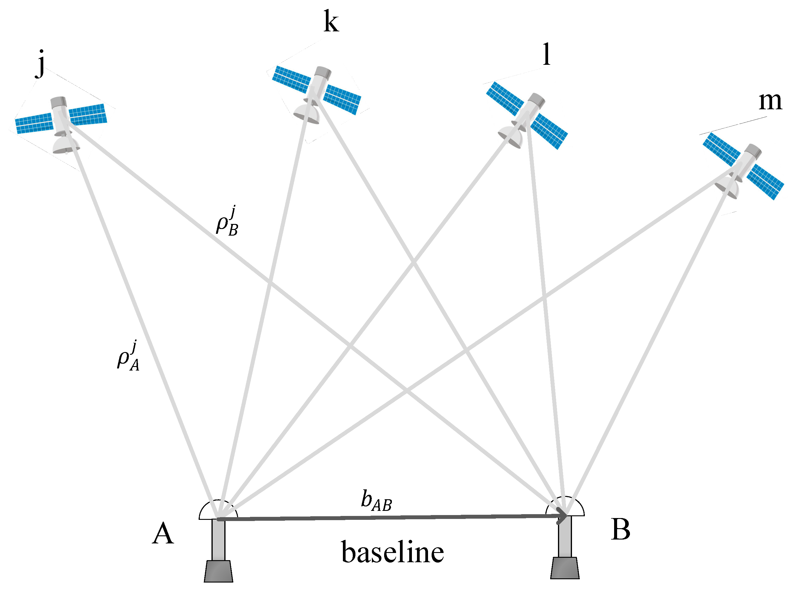
2.1. Real-Time Kinematic (RTK)
- A standard least-squares adjustment is performed regardless of the integer constraints on the ambiguities. The ‘float’ solution can be obtained.
- The float ambiguities are used to compute the corresponding integer ambiguities using the integer least-square method.
- A test is performed to decide whether to accept the calculated integer ambiguities.
- The so-called fixed solution can be achieved by correcting the float solution of all other parameters with the integer ambiguities.
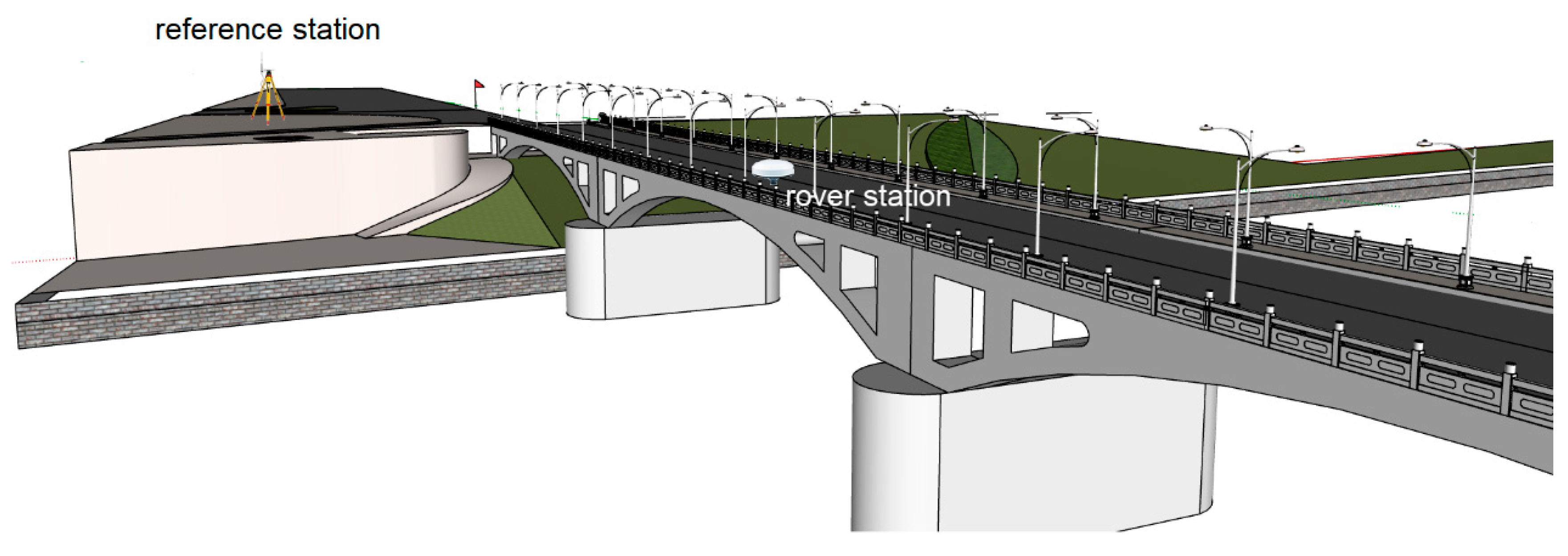
2.1.1. Application
- (1)
- A base station equipped with a geodetic GPS dual-frequency receiver was installed at a stable place nearby.
- (2)
- Two dual-frequency receivers were installed on the 66th floor of the Republic Plaza Building as rover stations.
- (3)
- A control center PC for running the monitoring software.
2.1.2. The Limitations of RTK-Based Dynamic Monitoring
- The reference station needs to be deployed at a stable place.
- When the reference station is also in the deformation zone, the method fails.
- The operation process is complicated and needs to be operated by professional surveying and mapping personnel.
- The reference and rover stations need to be observed at the same time, otherwise, no results will be obtained.
- The quality of the base station observation cannot be completely guaranteed, which will affect the positioning accuracy of the rover.
- The reference station receiver will increase monitoring costs.
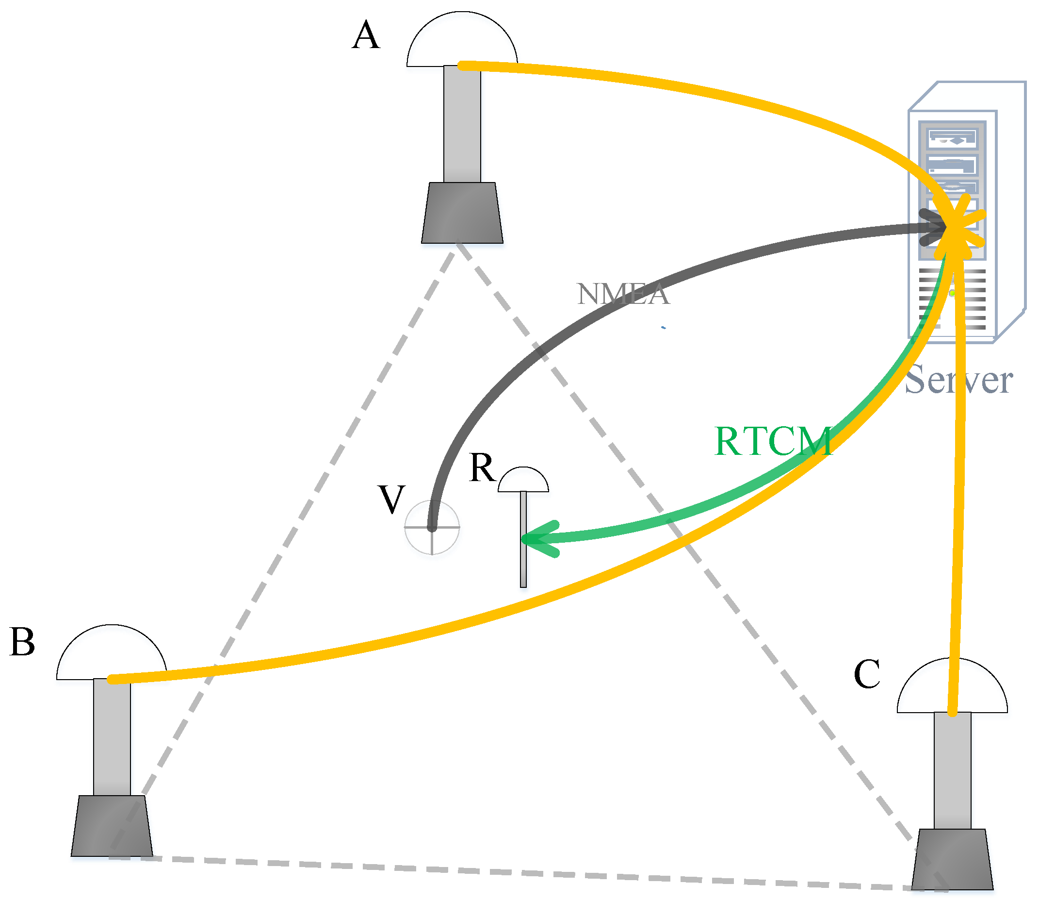
2.1.3. Network RTK
- (1)
- Data from the reference station network is transferred to the server for computing the models of orbital, ionospheric, tropospheric errors in .
- (2)
- The carrier phase ambiguities of the network baselines can be fixed and the actual error of network baselines can be calculated.
- (3)
- The approximate position of the user receiver obtained by standard point positioning (SPP) with code measurements is usually adopted as the coordinate of the VRS .
- (4)
- The VRS coordinate is transferred to the server, and linear or more sophisticated models are used to predict the errors at the VRS.
- (5)
- The observation of VRS is generated by Equation (6) and transmitted to the user receiver in standard format.
- (6)
- The relative positioning is adopted to calculate the position of user receiver.
- Users do not need to set up a reference station, the operation is simpler and faster.
- All users use a unified reference coordinate frame.
- Network RTK coverage is broader than that of traditional RTK [35].
- Network modeling for atmospheric correction.
- If the reference station is dense enough, the accuracy of the traditional RTK short baseline can be achieved.
- If there is a problem with one of the reference stations, the service can continue to be available. Network RTK has higher reliability and availability [42].
- Reduced user costs from a broad application perspective.
2.2. Precise Point Position (PPP)
2.3. Displacement versus Position
2.3.1. Variometric Approach for Displacements Analysis Stand-Alone Engine (VADASE)
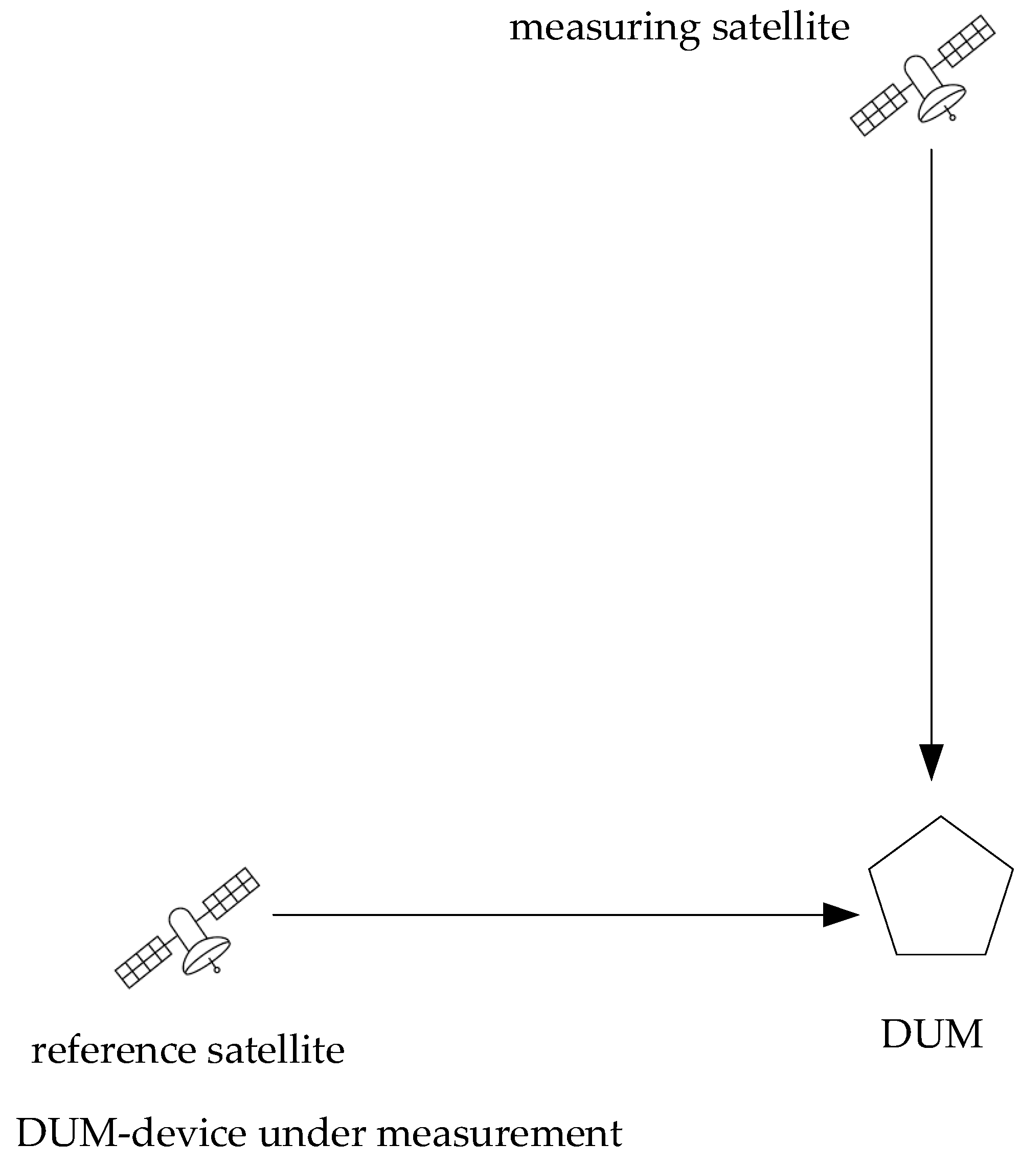
2.3.2. Phase Residual Method (PRM)
- Select a pair of satellites as reference satellite and measurement satellite according to the criteria.
- Compute the double difference carrier phase observation by Equation (17).
- Compute the phase residual by Equation (18).
- Perform FFT band filtering to clean the phase residuals.
2.3.3. Signal Processing Method (SPM)
- (1)
- Compute the double difference carrier phase observation at time .
- (2)
- High-pass filtering of the double-difference carrier phase observation sequence to remove long-term trend:where is the double difference carrier phase observation between receivers , and satellites , at time .
- (3)
- Calculate the azimuth and elevation angle of the satellite relative to the receiver at time t to form an observation equation.
- (4)
- Estimate () by the least squares method.
2.3.4. The Comparison of the Three Displacement Measurement Methods for SHM
- Easy implementation.
- Low computational overhead.
- No need to consider multi-system system bias.
- No need to consider multi-system frequency offset.
2.4. Single Frequency
2.5. Comparison of Different Technologies for Dynamic Monitoring
3. Improvement of GNSS-Based Dynamic Monitoring Technologies for SHM
3.1. Multiple Constellations
3.2. High-Rate GNSS Receiver
3.2.1. Error Characteristics
3.2.2. Application
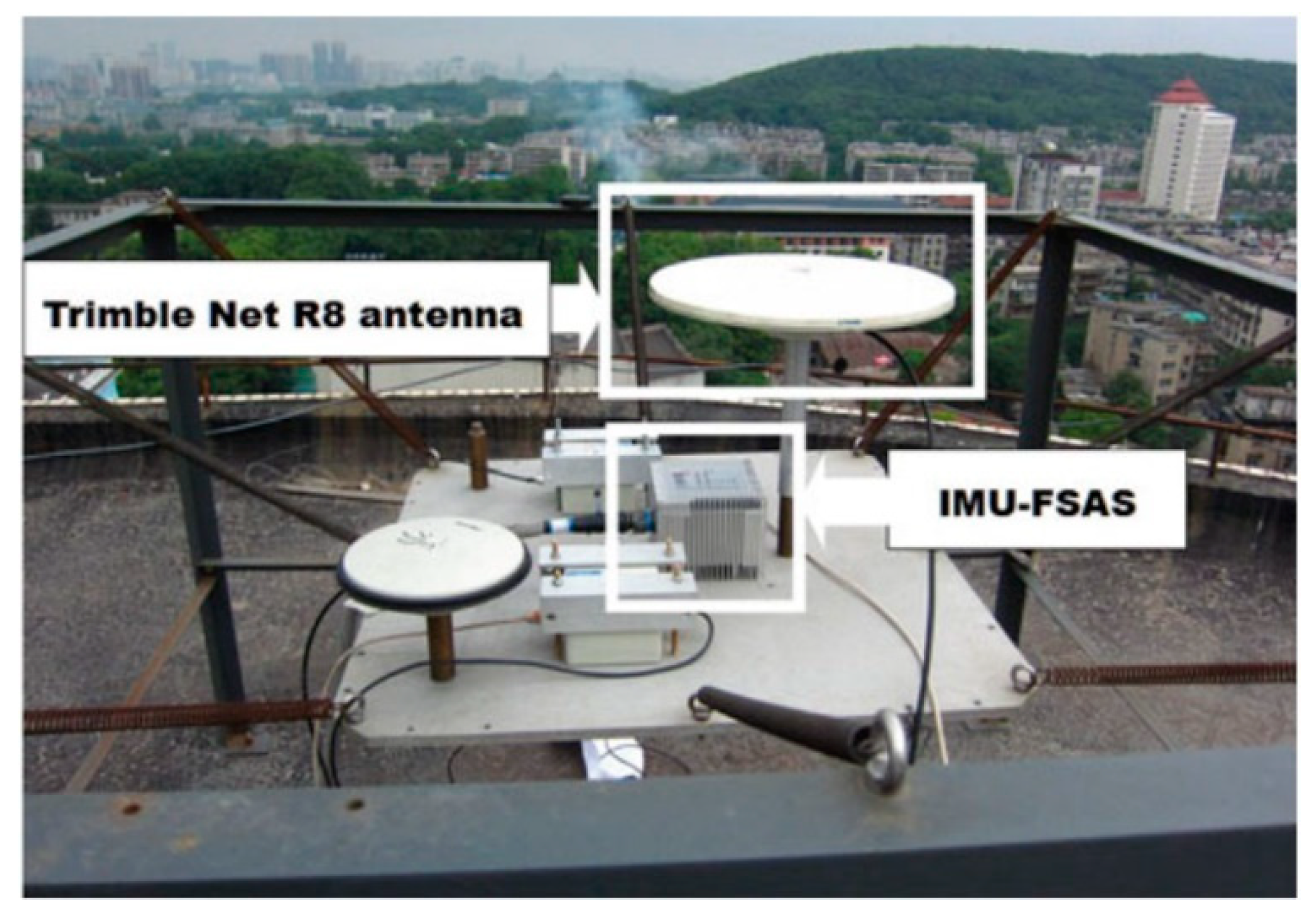
3.3. GNSSs & Accelerometers
3.3.1. Time Synchronization
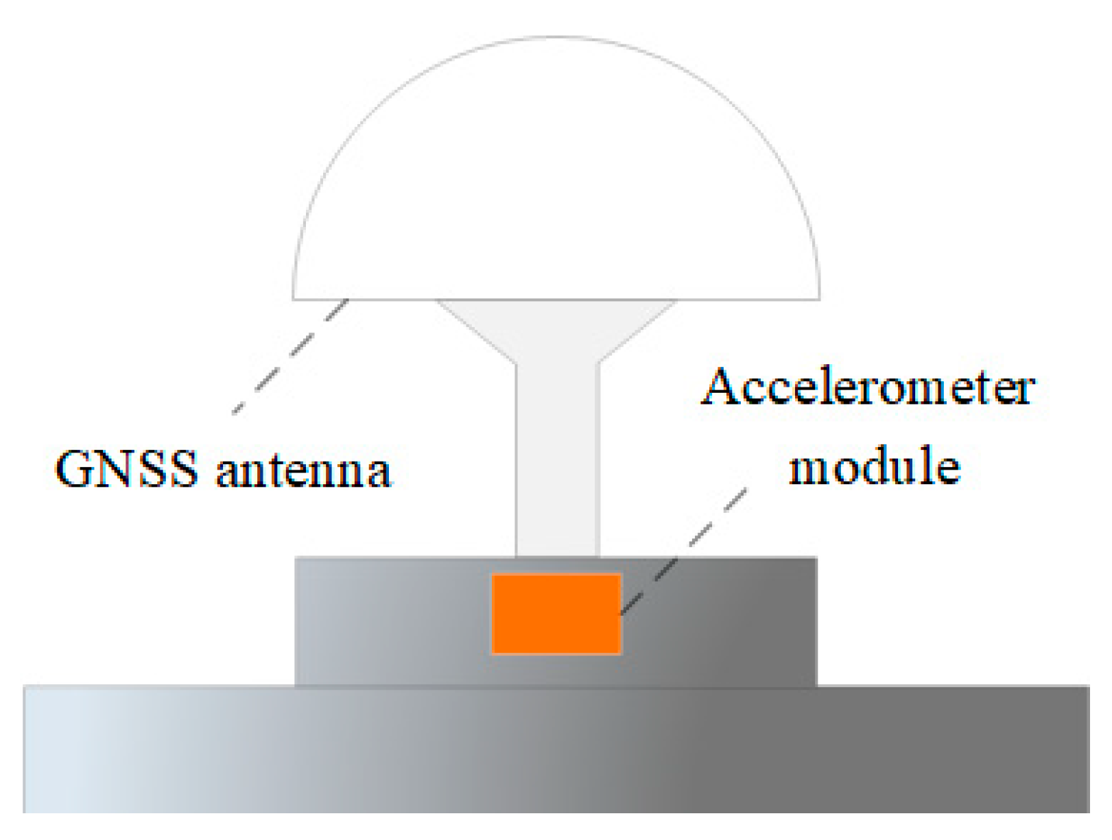
3.3.2. Integrated Design of the GNSS Antenna and Accelerometer
3.3.3. Data Fusion
Isolated Method
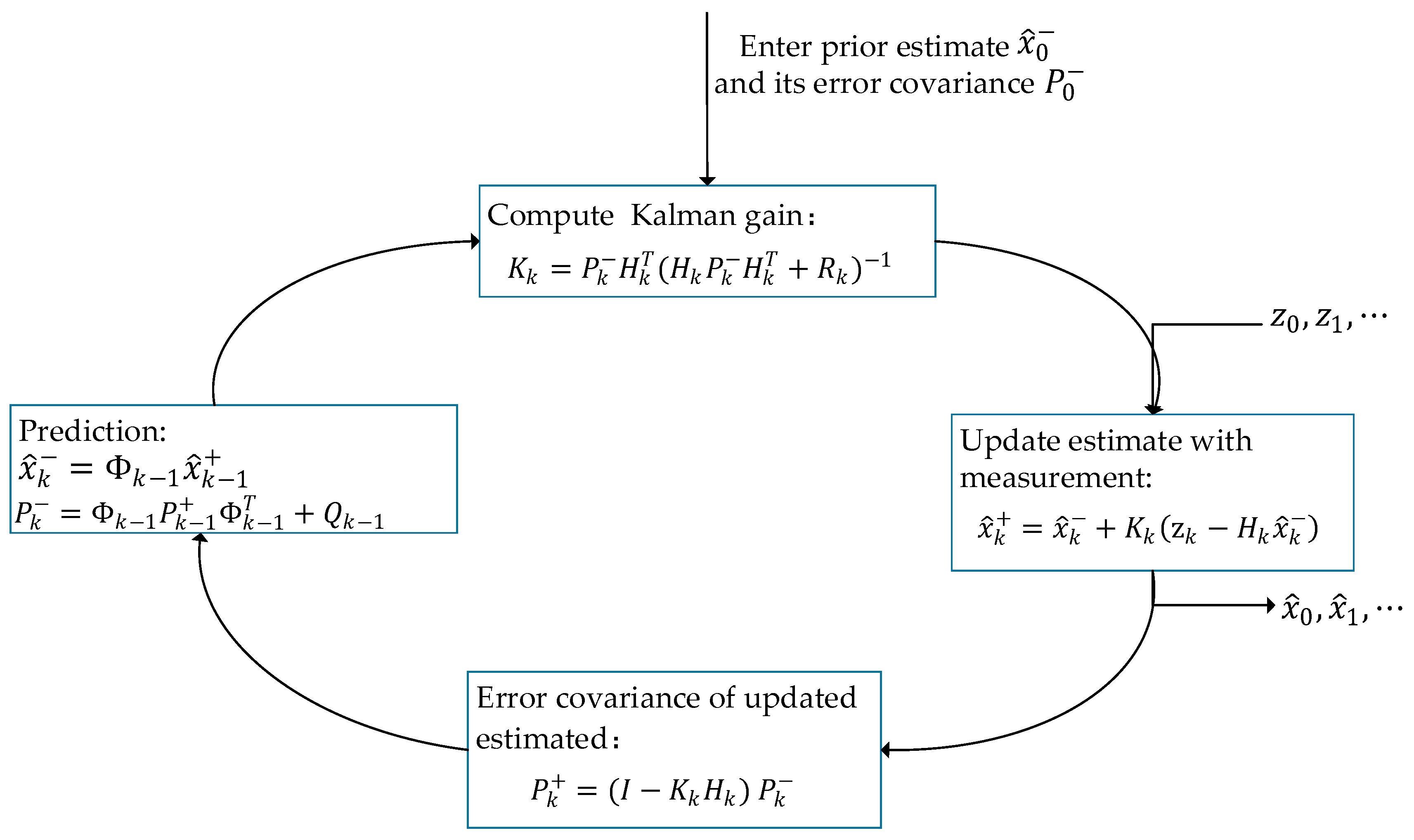
Kalman Filtering
4. Denoising and Detrending
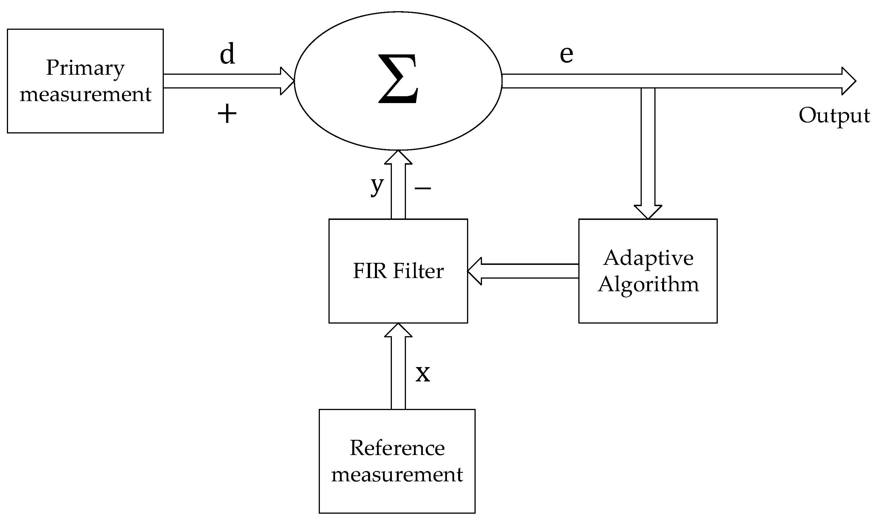
4.1. Adaptive Finite-Duration Impulse Response Filter (AF)
4.1.1. Theory
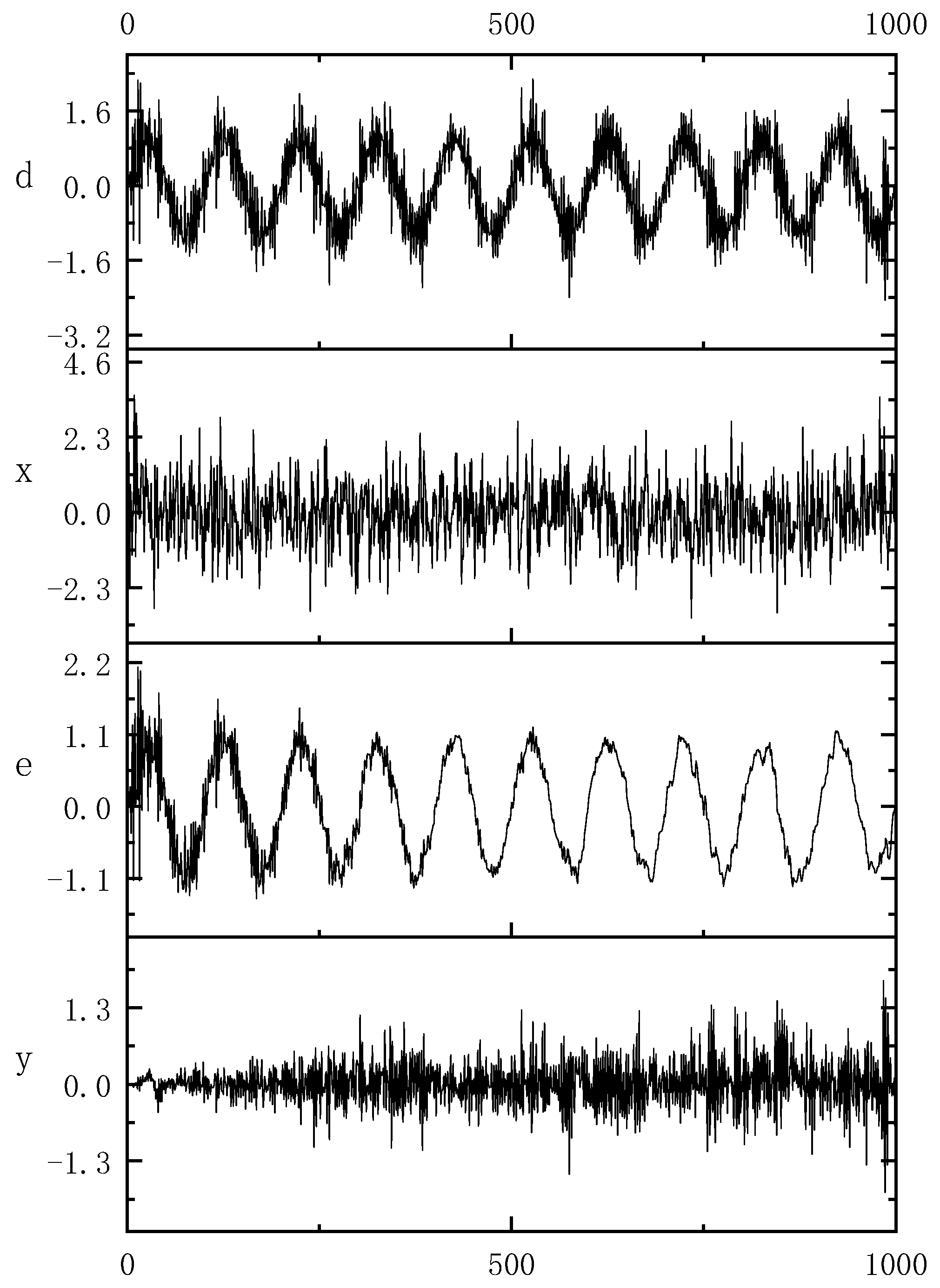
4.1.2. Application
4.2. Wavelet
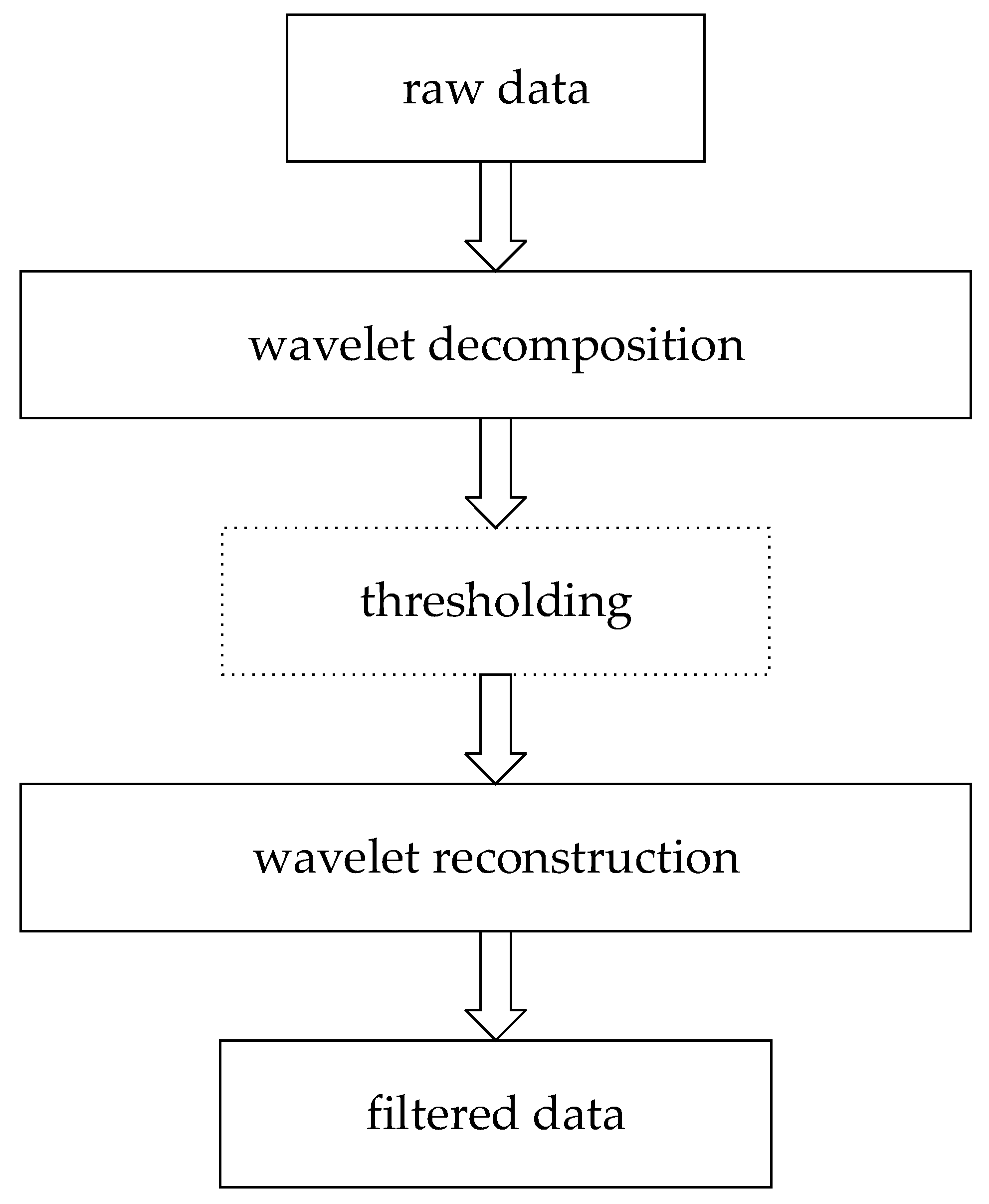
4.2.1. Theory
4.2.2. Application
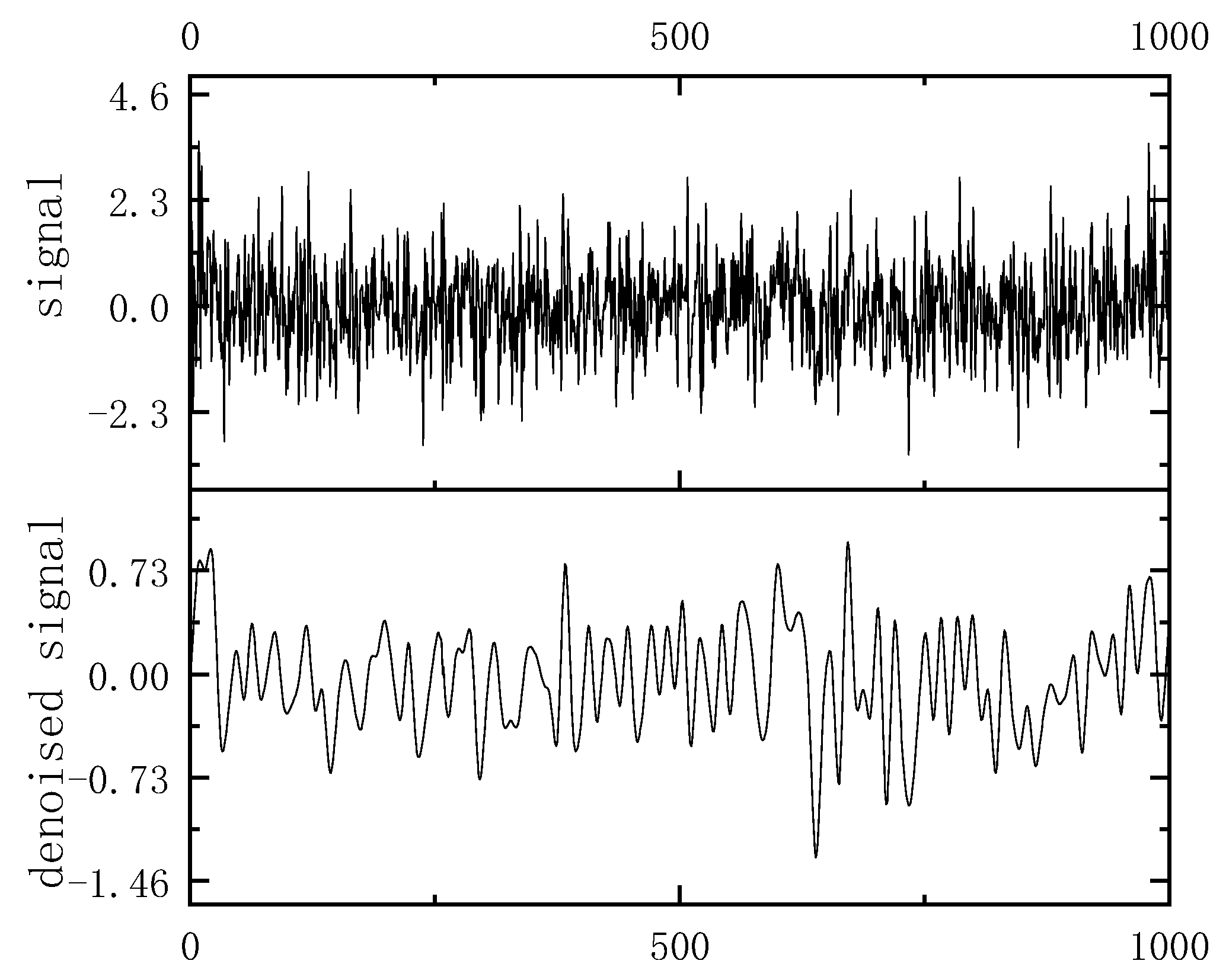
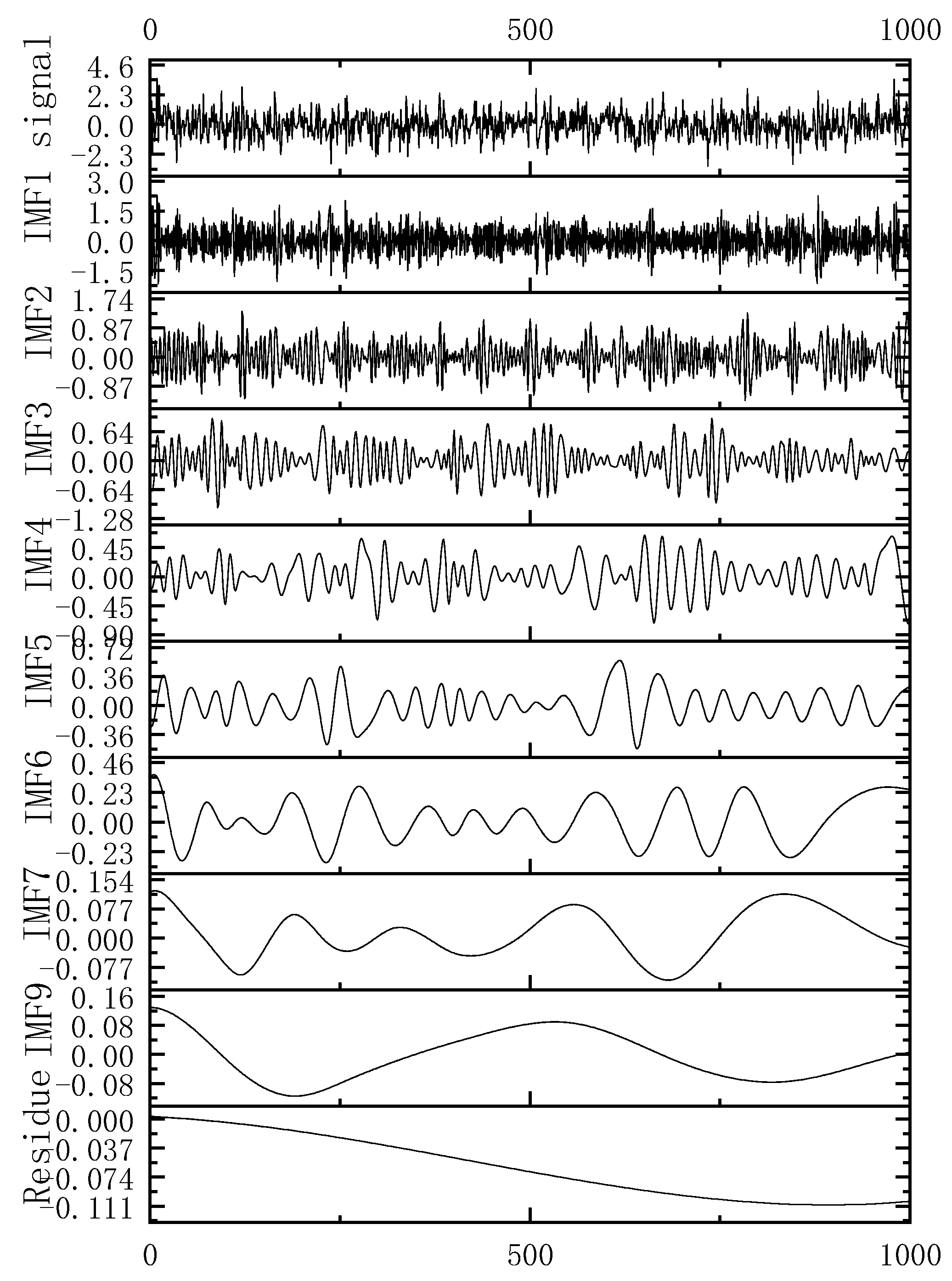
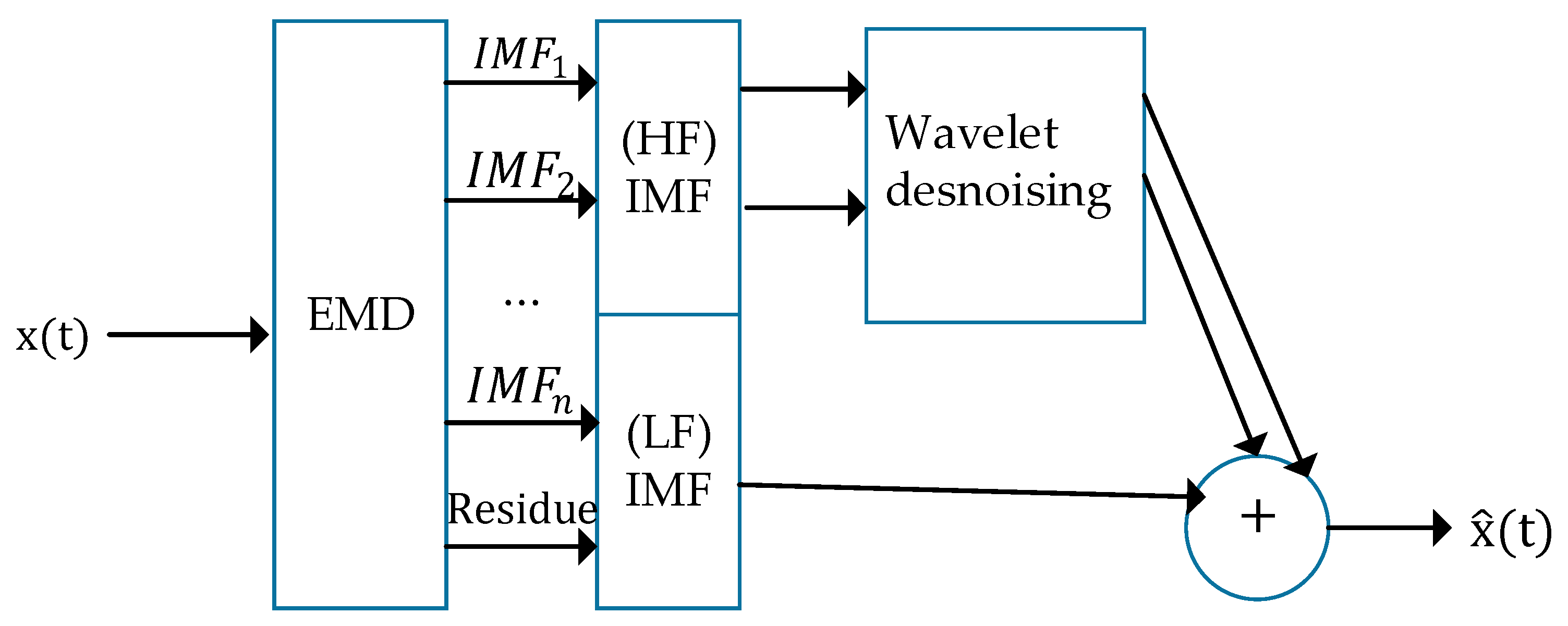
4.3. Empirical Mode Decomposition (EMD)
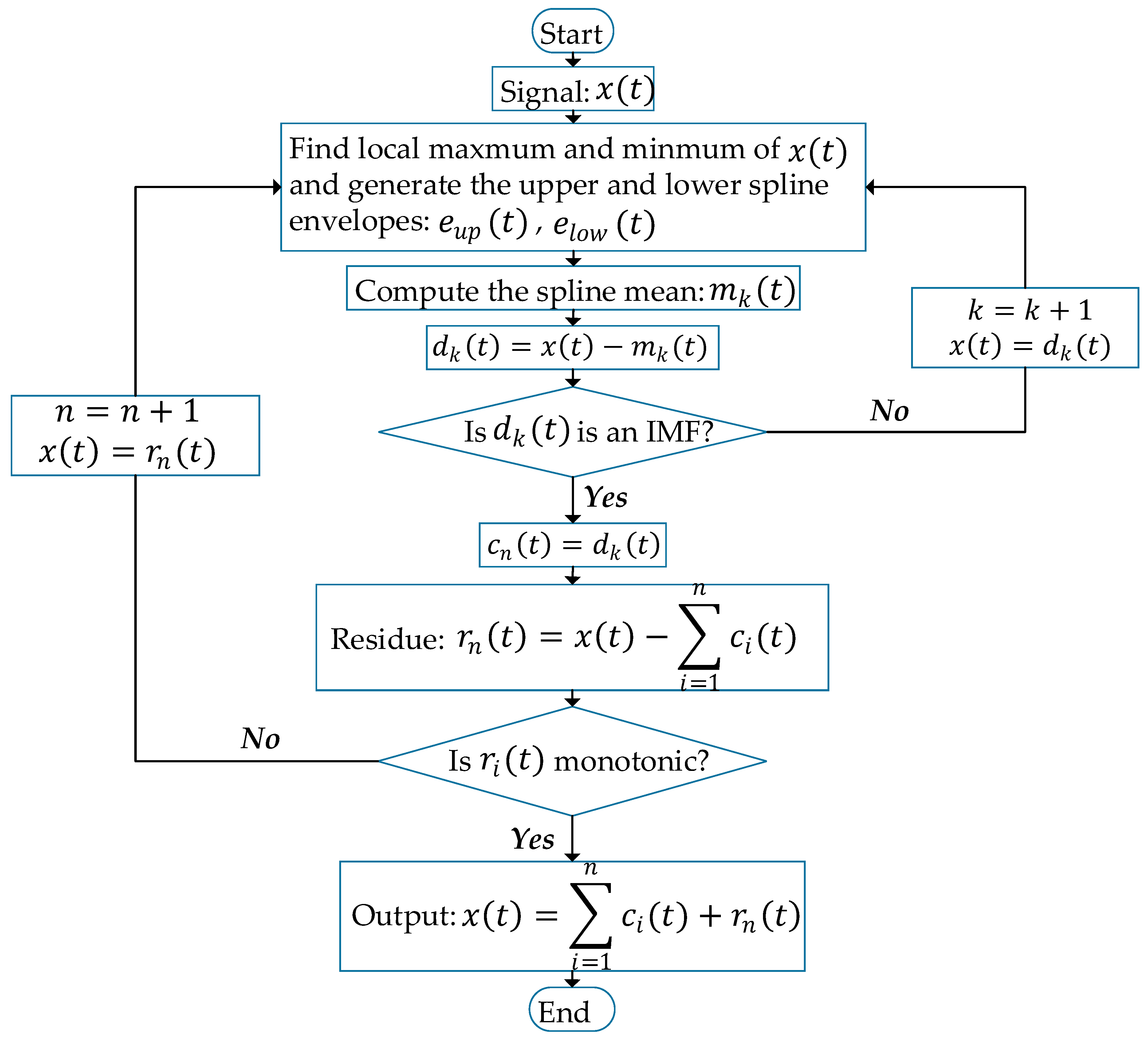
4.3.1. Theory
- (1)
- Find out the local maximum and minimum of the signal , and the upper spline envelope and the lower spline envelope can be generated by using these extreme points, where denotes time.
- (2)
- Computing the means of upper and lower envelopes:where denotes the loop index for calculating an IMF component.
- (3)
- The difference between and is calculated as:
- (4)
- is verified to satisfy the conditions of IMF: (a) the number of extrema and the number of zero crossings are equal or at most differ by one in the entire signal; (b) is zero for the entire signal. If these conditions are not met, is adopted as the new ‘’ and the steps (1)–(4) are repeated to calculate the nth IMF component. If these conditions are satisfied, is adopted as the IMF component: , where is the nth IMF component of original signal.
- (5)
- The nth residual is calculated as:
- (6)
- If the is not monotonic, the is adopted as the new ‘, and steps (1)–(6) are repeated to calculated the next IMF component. If the is monotonic, the entire decomposition process is terminated, the original signal can be expressed as:
4.3.2. Application
5. Conclusions
- Currently, most receivers on the market support multi-GNSS and multi-frequencies. More research using controlled trials is needed to be done to evaluate the accuracy and reliability it can be achieved in its application for SHM.
- Network RTK technology is an effective means to reduce the cost of large-scale SHM applications from the coverage perspective, and further research is needed to study the achievable monitoring accuracy within network coverage.
- At present, the fusion of GNSS and other sensors for SHM is a loose combination, and the tight fusion between them needs further research. In addition, further research should be undertaken to investigate the cost and precision of multi-sensor fusion for SHM.
- Currently, PPP-based dynamic monitoring for SHM is based on IGS precise ephemeris and clock products. The PPP-based dynamic monitoring for SHM based on real-time data stream service remains to be studied.
Author Contributions
Funding
Acknowledgments
Conflicts of Interest
References
- Farrar, C.R.; Worden, K. An introduction to structural health monitoring. Philos. Trans. R. Soc. A Math. Phys. Eng. Sci. 2006, 365, 303–315. [Google Scholar] [CrossRef]
- Sohn, H.; Farrar, C.R.; Hemez, F.M.; Shunk, D.D.; Stinemates, D.W.; Nadler, B.R.; Czarnecki, J.J. A review of structural health monitoring literature: 1996–2001. In Proceedings of the Third World Conference on Structural Control, Como, Italy, 7–12 April 2002. [Google Scholar]
- Manzini, N.; Orcesi, A.; Thom, C.; Clément, A.; Botton, S.; Ortiz, M.; Dumoulin, J.; Mandé, F. Structural Health Monitoring using a GPS sensor network. In Proceedings of the 9th European Workshop on Structural Health Monitoring Series (EWSHM), Manchester, UK, 10–13 July 2018; p. 12. [Google Scholar]
- Moss, R.; Matthews, S. In-service structural monitoring a state of the art review. Struct. Eng. 1995, 73, 23–31. [Google Scholar]
- Mita, A.; Takhira, S. A smart sensor using a mechanical memory for structural health monitoring of a damage-controlled building. Smart Mater. Struct. 2003, 12, 204. [Google Scholar] [CrossRef]
- Brownjohn, J.M. Structural health monitoring of civil infrastructure. Philos. Trans. A Math. Phys. Eng. Sci. 2007, 365, 589–622. [Google Scholar] [CrossRef] [PubMed]
- Chang, F.-K. Structural Health Monitoring 2003: From Diagnostics & Prognostics to Structural Health Management. In Proceedings of the 4th International Workshop on Structural Health Monitoring, Stanford, CA, USA, 15–17 September 2003; DEStech Publications, Inc.: Lancaster, PA, USA, 2003; pp. 499–506. [Google Scholar]
- Ogaja, C.; Li, X.; Rizos, C. Advances in structural monitoring with global positioning system technology: 1997–2006. J. Appl. Geod. JAG 2007, 1, 171–179. [Google Scholar] [CrossRef]
- Yi, T.; Li, H.; Gu, M. Recent research and applications of GPS based technology for bridge health monitoring. Sci. China Technol. Sci. 2010, 53, 2597–2610. [Google Scholar] [CrossRef]
- Yi, T.; Li, H.; Gu, M. Full-scale measurements of dynamic response of suspension bridge subjected to environmental loads using GPS technology. Sci. China Technol. Sci. 2010, 53, 469–479. [Google Scholar] [CrossRef]
- Im, S.B.; Hurlebaus, S.; Kang, Y.J. Summary review of GPS technology for structural health monitoring. J. Struct. Eng. 2011, 139, 1653–1664. [Google Scholar] [CrossRef]
- Rizos, C. Trends in GPS Technology & Applications. In Proceedings of the 2nd International LBS Workshop, Boston, MA, USA, 4 April 2009; Available online: http://citeseerx.ist.psu.edu/viewdoc/download?doi=10.1.1.640.3051&rep=rep1&type=pdf (accessed on 12 April 2019).
- Dorides, C.D. GNSS User Technology Report; European GNSS Agency: Holešovice, Czechia, 2018; pp. 60–61. Available online: https://www.gsa.europa.eu/system/files/reports/gnss_user_tech_report_2018.pdf (accessed on 12 April 2019).
- Wang, L.; Chen, R.; Li, D.; Zhang, G.; Shen, X.; Yu, B.; Wu, C.; Xie, S.; Zhang, P.; Li, M.; et al. Initial Assessment of the LEO Based Navigation signal augmentation System from Luojia-1A Satellite. Sensors 2018, 18, 3919. [Google Scholar] [CrossRef] [PubMed]
- Bock, Y.; Prawirodirdjo, L.; Melbourne, T.I. Detection of arbitrarily large dynamic ground motions with a dense high-rate GPS network. Geophys. Res. Lett. 2004, 31, L06604. [Google Scholar]
- Choi, K.; Bilich, A.; Larson, K.M.; Axelrad, P. Modified sidereal filtering: Implications for high-rate GPS positioning. Geophys. Res. Lett. 2004, 31. [Google Scholar] [CrossRef]
- Hofmann-Wellenhof, B.; Lichtenegger, H.; Wasle, E. GNSS–Global Navigation Satellite Systems: GPS, GLONASS, Galileo, and More; Springer Science & Business Media: Berlin/Heidelberg, Germany, 2007; pp. 161–191. [Google Scholar]
- Vollath, U.; Birnbach, S.; Landau, L.; Fraile-Ordoñez, J.M.; Martí-Neira, M. Analysis of Three-Carrier Ambiguity Resolution Technique for Precise Relative Positioning in GNSS-2. Navigation 1999, 46, 13–23. [Google Scholar] [CrossRef]
- Leick, A.; Rapoport, L.; Tatarnikov, D. GPS Satellite Surveying; John Wiley & Sons: Hoboken, NJ, USA, 2015; pp. 257–357. [Google Scholar]
- Teunissen, P.J. The least-squares ambiguity decorrelation adjustment: A method for fast GPS integer ambiguity estimation. J. Geod. 1995, 70, 65–82. [Google Scholar] [CrossRef]
- Teunissen, P.; Joosten, P.; Tiberius, C. Geometry-free ambiguity success rates in case of partial fixing. In Proceedings of the 1999 National Technical Meeting of The Institute of Navigation, San Diego, CA, USA, 25–27 January 1999; pp. 201–207. [Google Scholar]
- Teunissen, P.; Verhagen, S. GNSS carrier phase ambiguity resolution: Challenges and open problems. In Observing Our Changing Earth; Springer: Berlin/Heidelberg, Germany, 2009; pp. 785–792. [Google Scholar]
- Wang, L.; Verhagen, S. A new ambiguity acceptance test threshold determination method with controllable failure rate. J. Geod. 2015, 89, 361–375. [Google Scholar] [CrossRef]
- Wang, L.; Feng, Y.; Guo, J. Reliability control of single-epoch RTK ambiguity resolution. GPS Solut. 2016, 21, 591–604. [Google Scholar] [CrossRef]
- Ogaja, C.; Rizos, C.; Wang, J.; Brownjohn, J. Toward the implementation of on-line structural monitoring using RTK-GPS and analysis of results using the wavelet transform. In Proceedings of the 10th FIG International Symposium on Deformation Measurements, Orange, CA, USA, 19–22 March 2001; pp. 19–22. [Google Scholar]
- Ashkenazi, V.; Dodson, A.; Moore, T.; Roberts, G. Real time OTF GPS monitoring of the Humber Bridge. Surv. World 1996, 4, 26–28. [Google Scholar]
- Ashkenazi, V.; Roberts, G. Experimental monitoring of the Humber Bridge using GPS. In Institution of Civil Engineers-Civil Engineering; Thomas Telford-ICE Virtual Library: London, UK, 1997; pp. 177–182. [Google Scholar]
- Roberts, G.; Meng, X.; Dodson, A. The use of kinematic GPS and triaxial accelerometers to monitor the deflections of large bridges. In Proceedings of the 10th FIG International Symposium on Deformation Measurement, Orange, CA, USA, 19–22 March 2001; pp. 19–22. [Google Scholar]
- Roberts, G.W.; Cosser, E.; Meng, X.; Dodson, A. High frequency deflection monitoring of bridges by GPS. Positioning 2004, 1, 226–231. [Google Scholar] [CrossRef]
- Roberts, G.W.; Dodson, A.; Brown, C.; Karunar, R.; Evans, A. Monitoring the height deflections of the Humber Bridge by GPS, GLONASS, and finite element modelling. In Geodesy Beyond 2000; Springer: Berlin/Heidelberg, Germany, 2000; pp. 355–360. [Google Scholar]
- Dodson, A.; Meng, X.; Roberts, G. Adaptive method for multipath mitigation and its applications for structural deflection monitoring. In Proceedings of the International Symposium on Kinematic Systems in Geodesy, Geomatics and Navigation (KIS 2001), Banff, AB, Canada, 5–8 June 2001; pp. 101–110. [Google Scholar]
- Meng, X. Real-Time Deformation Monitoring of Bridges Using GPS/Accelerometers. Ph.D. Thesis, University of Nottingham, Nottingham, UK, 2002. [Google Scholar]
- Meng, X.; Roberts, G.W.; Cosser, E.; Dodson, A.H.; Barnes, J.; Rizos, C. Real-time bridge deflection and vibration monitoring using an integrated GPS/accelerometer/pseudolite system. In Proceedings of the 11th International Symposium on Deformation Measurements, International Federation Surveyors (FIG), Commission 6-Engineering Surveys, Working Group, Santorini, Greece, 25–28 May 2003. [Google Scholar]
- Meng, X.; Roberts, G.; Henry Roberts, A.; Dodson, S.; Ince, S.; Waugh, S. GNSS for structural deformation and deflection monitoring: Implementation and data analysis. In Proceedings of the 3rd IAG/12th FIG Symposium, Baden, Germany, 22–24 May 2006; pp. 22–24. [Google Scholar]
- Vollath, U.; Landau, H.; Chen, X.; Doucet, K.; Pagels, C. Network RTK versus single base RTK–understanding the error characteristics. In Proceedings of the 15th International Technical Meeting of the Satellite Division of the Institute of Navigation, Portland, OR, USA, 24–27 September 2002; pp. 24–27. [Google Scholar]
- Rizos, C. Network RTK research and implementation: A geodetic perspective. J. Glob. Position. Syst. 2002, 1, 144–150. [Google Scholar] [CrossRef]
- Landau, H.; Vollath, U.; Chen, X. Virtual reference stations versus broadcast solutions in network RTK–advantages and limitations. In Proceedings of the GNSS 2003 European Navigation Conference, Graz, Austria, 22–25 April 2003. [Google Scholar]
- Pepe, M. CORS architecture and evaluation of positioning by low-cost GNSS receiver. Geod. Cartogr. 2018, 44, 36–44. [Google Scholar] [CrossRef]
- Stempfhuber, W. 3D-RTK capability of single GNSS receivers. Int. Arch. Photogramm. Remote Sens. Spat. Inf. Sci. 2013, 40, 379–384. [Google Scholar] [CrossRef]
- Wübbena, G.; Bagge, A.; Schmitz, M. Network Based Techniques for RTK Applications. GPS JIN 2001, 14–16. [Google Scholar]
- Vollath, U.; Landau, H.; Chen, X. Network RTK–concept and performance. In Proceedings of the GNSS Symposium, Wuhan, China, 27–30 May 2002. [Google Scholar]
- Vollath, U.; Buecherl, A.; Landau, H.; Pagels, C.; Wagner, B. Multi-base RTK positioning using virtual reference stations. In Proceedings of the ION GPS, Salt Lake City, UT, USA, 19–22 September 2000; pp. 123–131. [Google Scholar]
- Yu, J.; Yan, B.; Meng, X.; Shao, X.; Ye, H. Measurement of bridge dynamic responses using network-based real-time kinematic GNSS technique. J. Surv. Eng. 2016, 142, 04015013. [Google Scholar] [CrossRef]
- Yu, J.; Meng, X.; Shao, X.; Yan, B.; Yang, L. Identification of dynamic displacements and modal frequencies of a medium-span suspension bridge using multimode GNSS processing. Eng. Struct. 2014, 81, 432–443. [Google Scholar] [CrossRef]
- Moschas, F.; Stiros, S. Measurement of the dynamic displacements and of the modal frequencies of a short-span pedestrian bridge using GPS and an accelerometer. Eng. Struct. 2011, 33, 10–17. [Google Scholar] [CrossRef]
- Kaloop, M.; Hu, J.; Elbeltagi, E. Adjustment and Assessment of the Measurements of Low and High Sampling Frequencies of GPS Real-Time Monitoring of Structural Movement. ISPRS Int. J. Geo-Inf. 2016, 5, 222. [Google Scholar] [CrossRef]
- Kaloop, M.R.; Hu, J.W. Dynamic Performance Analysis of the Towers of a Long-Span Bridge Based on GPS Monitoring Technique. J. Sens. 2016, 2016, 7494817. [Google Scholar] [CrossRef]
- Elnabwy, M.T.; Kaloop, M.R.; Elbeltagi, E. Talkha steel highway bridge monitoring and movement identification using RTK-GPS technique. Measurement 2013, 46, 4282–4292. [Google Scholar] [CrossRef]
- Bisnath, S.; Gao, Y. Precise point positioning. GPS World 2009, 20, 43–50. [Google Scholar]
- Bisnath, S.; Gao, Y. Current state of precise point positioning and future prospects and limitations. In Observing Our Changing Earth; Springer: Berlin/Heidelberg, Germany, 2009; pp. 615–623. [Google Scholar]
- Zumberge, J.; Heflin, M.; Jefferson, D.; Watkins, M.; Webb, F. Precise point positioning for the efficient and robust analysis of GPS data from large networks. J. Geophys. Res. Solid Earth 1997, 102, 5005–5017. [Google Scholar] [CrossRef]
- Kouba, J.; Héroux, P. Precise point positioning using IGS orbit and clock products. GPS Solut. 2001, 5, 12–28. [Google Scholar] [CrossRef]
- Teunissen, P.; Khodabandeh, A. Review and principles of PPP-RTK methods. J. Geod. 2015, 89, 217–240. [Google Scholar] [CrossRef]
- Shen, X. Improving Ambiguity Convergence in Carrier Phase-Based Precise Point Positioning. Ph.D. Thesis, Department of Geomatics Engineering, University of Calgary, Calgary, AB, Canada, 2002. [Google Scholar]
- Witchayangkoon, B. Elements of GPS Precise Point Positioning. Ph.D. Thesis, Spatial Information Science and Engineering, University of Maine, Orono, ME, USA, 2000. [Google Scholar]
- Xu, P.; Shi, C.; Fang, R.; Liu, J.; Niu, X.; Zhang, Q.; Yanagidani, T. High-rate precise point positioning (PPP) to measure seismic wave motions: An experimental comparison of GPS PPP with inertial measurement units. J. Geod. 2013, 87, 361–372. [Google Scholar] [CrossRef]
- Yigit, C.O.; Gurlek, E. Experimental testing of high-rate GNSS precise point positioning (PPP) method for detecting dynamic vertical displacement response of engineering structures. Geomat. Nat. Hazards Risk 2017, 8, 893–904. [Google Scholar] [CrossRef]
- Xu, C.-H.; Wang, J.-L.; Gao, J.-X.; Jian, W.; Hong, H. Precise point positioning and its application in mining deformation monitoring. Trans. Nonferrous Met. Soc. China 2011, 21, s499–s505. [Google Scholar] [CrossRef]
- Hu, H.; Gao, J.; Yao, Y. Land deformation monitoring in mining area with PPP-AR. Int. J. Min. Sci. Technol. 2014, 24, 207–212. [Google Scholar] [CrossRef]
- Martín, A.; Anquela, A.B.; Dimas-Pagés, A.; Cos-Gayón, F. Validation of performance of real-time kinematic PPP. A possible tool for deformation monitoring. Measurement 2015, 69, 95–108. [Google Scholar] [CrossRef]
- Song, W.; Zhang, R.; Yao, Y.; Liu, Y.; Hu, Y. PPP Sliding Window Algorithm and Its Application in Deformation Monitoring. Sci. Rep. 2016, 6, 26497. [Google Scholar] [CrossRef] [PubMed]
- Paziewski, J.; Sieradzki, R.; Baryla, R. Multi-GNSS high-rate RTK, PPP and novel direct phase observation processing method: Application to precise dynamic displacement detection. Meas. Sci. Technol. 2018, 29, 035002. [Google Scholar] [CrossRef]
- Yigit, C.O. Experimental assessment of post-processed kinematic Precise Point Positioning method for structural health monitoring. Geomat. Nat. Hazards Risk 2016, 7, 360–383. [Google Scholar] [CrossRef]
- Moschas, F.; Avallone, A.; Saltogianni, V.; Stiros, S.C. Strong motion displacement waveforms using 10-Hz precise point positioning GPS: An assessment based on free oscillation experiments. Earthq. Eng. Struct. Dyn. 2014, 43, 1853–1866. [Google Scholar] [CrossRef]
- Shi, C.; Lou, Y.-D.; Zhang, H.-P.; Zhao, Q.; Geng, J.; Wang, R.; Fang, R.; Liu, J. Seismic deformation of the Mw 8.0 Wenchuan earthquake from high-rate GPS observations. Adv. Space Res. 2010, 46, 228–235. [Google Scholar] [CrossRef]
- Kaloop, M.R.; Rabah, M. Time and frequency domains response analyses of April 2015 Greece’s earthquake in the Nile Delta based on GNSS-PPP. Arab. J. Geosci. 2016, 9, 316. [Google Scholar] [CrossRef]
- Colosimo, G.; Crespi, M.; Mazzoni, A. Real-time GPS seismology with a stand-alone receiver: A preliminary feasibility demonstration. J. Geophys. Res. Solid Earth 2011, 116, B11302. [Google Scholar] [CrossRef]
- Benedetti, E.; Branzanti, M.; Biagi, L.; Colosimo, G.; Mazzoni, A.; Crespi, M. Global Navigation Satellite Systems seismology for the 2012 M w 6.1 Emilia earthquake: Exploiting the VADASE algorithm. Seismol. Res. Lett. 2014, 85, 649–656. [Google Scholar] [CrossRef]
- Branzanti, M.; Colosimo, G.; Crespi, M.; Mazzoni, A. GPS near-real-time coseismic displacements for the great Tohoku-oki earthquake. IEEE Geosci. Remote Sens. Lett. 2013, 10, 372–376. [Google Scholar] [CrossRef]
- Hung, H.-K.; Rau, R.-J.; Benedetti, E.; Branzanti, M.; Mazzoni, A.; Colosimo, G.; Crespi, M. GPS Seismology for a moderate magnitude earthquake: Lessons learned from the analysis of the 31 October 2013 ML 6.4 Ruisui (Taiwan) earthquake. Ann. Geophys. 2017, 60, 0553. [Google Scholar] [CrossRef]
- Geng, T.; Xie, X.; Fang, R.; Su, X.; Zhao, Q.; Liu, G.; Li, H.; Shi, C.; Liu, J. Real-time capture of seismic waves using high-rate multi-GNSS observations: Application to the 2015 Mw 7.8 Nepal earthquake. Geophys. Res. Lett. 2016, 43, 161–167. [Google Scholar] [CrossRef]
- Shu, Y.; Fang, R.; Li, M.; Shi, C.; Li, M.; Liu, J. Very high-rate GPS for measuring dynamic seismic displacements without aliasing: Performance evaluation of the variometric approach. GPS Solut. 2018, 22, 121. [Google Scholar] [CrossRef]
- Fratarcangeli, F.; Savastano, G.; D’Achille, M.; Mazzoni, A.; Crespi, M.; Riguzzi, F.; Devoti, R.; Pietrantonio, G. VADASE reliability and accuracy of real-time displacement estimation: Application to the Central Italy 2016 earthquakes. Remote Sens. 2018, 10, 1201. [Google Scholar] [CrossRef]
- Ashcroft, N.; Youssef, T.; Anthony, C. Leica VADASE: First Autonomous GNSS Monitoring Solution. Available online: http://www.fig.net/resources/proceedings/fig_proceedings/fig2016/papers/ts07b/TS07B_ashcroft_tawk_et_al_7952.pdf (accessed on 12 April 2019).
- Savastano, G.; Fratarcangeli, F.; Chiara D’Achille, M.; Mazzoni, A.; Crespi, M. Recent advances of VADASE to enhance reliability and accuracy of real-time displacements estimation. In Proceedings of the EGU General Assembly Conference Abstracts, Vienna, Austria, 23–28 April 2017; p. 11486. [Google Scholar]
- Benedetti, E.; Ravanelli, R.; Moroni, M.; Nascetti, A.; Crespi, M. Exploiting Performance of Different Low-Cost Sensors for Small Amplitude Oscillatory Motion Monitoring: Preliminary Comparisons in View of Possible Integration. J. Sens. 2016, 2016, 7490870. [Google Scholar] [CrossRef]
- Schaal, R.E.; Larocca, A.P.C. A Methodology for Monitoring Vertical Dynamic Sub-Centimeter Displacments with GPS. GPS Solut. 2002, 5, 15–18. [Google Scholar] [CrossRef]
- Larocca, A.P.C.; Schaal, R.E.; Guimarães, G. d. N.; da Silveira, I.M.; Segantine, P.C.L. Frequency Structures Vibration Identified by an Adaptative Filtering Techiques Applied on GPS L1 Signal. Positioning 2013, 4, 137. [Google Scholar] [CrossRef]
- Larocca, A.P.C. Using high-rate GPS data to monitor the dynamic behavior of a cable-stayed bridge. In Proceedings of the 17th International Technical Meeting of the Satellite Division of the US Institute of Navigation, Long Beach, CA, USA, 21–24 September 2004. [Google Scholar]
- Larocca, A.P.C.; Schaal, R.E.; Santos, M.; Langley, R. Monitoring the deflection of the Pierre-Laporte suspension bridge with the phase residual method. In Proceedings of the 18th International Technical Meeting of the Satellite Division of The Institute of Navigation, Long Beach, CA, USA, 13–16 September 2005; pp. 2023–2028. [Google Scholar]
- Larocca, A.P.C.; de Araújo Neto, J.O.; Trabanco, J.L.A.; dos Santos, M.C.; Barbosa, A.C.B. First Steps Using Two GPS Satellites for Monitoring the Dynamic Behavior of a Small Concrete Highway Bridge. J. Surv. Eng. 2016, 142, 04016008. [Google Scholar] [CrossRef]
- Larocca, A.P.C.; Neto, J.; Barbosa, A.; Trabanco, J.L.A.; Da Cunha, A.L.B.N. Dynamic Monitoring vertical Deflectionof Small Concrete Bridge Using Conventional Sensors And 100 Hz GPS Receivers—Preliminary Results. IOSR J. Eng. 2014, 4, 9–20. [Google Scholar] [CrossRef]
- Huang, S.; Wang, J. New data processing strategy for single frequency GPS deformation monitoring. Surv. Rev. 2015, 47, 379–385. [Google Scholar] [CrossRef]
- Jiang, W.; Zou, X.; Tang, W. A New Kind of Real-Time PPP Method for GPS Single-Frequency Receiver Using CORS Network. Chin. J. Geophys. 2012, 55, 284–293. [Google Scholar] [CrossRef]
- Odijk, D.; Teunissen, P.J.; Zhang, B. Single-frequency integer ambiguity resolution enabled GPS precise point positioning. J. Surv. Eng. 2012, 138, 193–202. [Google Scholar] [CrossRef]
- Zou, X.; Ge, M.; Tang, W.; Shi, C.; Liu, J. URTK: Undifferenced network RTK positioning. GPS Solut. 2013, 17, 283–293. [Google Scholar] [CrossRef]
- Cosser, E.; Roberts, G.W.; Meng, X.; Dodson, A.H. The comparison of single frequency and dual frequency GPS for bridge deflection and vibration monitoring. In Proceedings of the Deformation Measurements and Analysis, 11th International Symposium on Deformation Measurements, International Federation of Surveyors (FIG), Commission 6-Engineering Surveys, Working Group 6.1, Santorini, Greece, 25–28 May 2003. [Google Scholar]
- He, H.; Li, J.; Yang, Y.; Xu, J.; Guo, H.; Wang, A. Performance assessment of single-and dual-frequency BeiDou/GPS single-epoch kinematic positioning. GPS Solut. 2014, 18, 393–403. [Google Scholar] [CrossRef]
- Koo, G.; Kim, K.; Chung, J.Y.; Choi, J.; Kwon, N.Y.; Kang, D.Y.; Sohn, H. Development of a High Precision Displacement Measurement System by Fusing a Low Cost RTK-GPS Sensor and a Force Feedback Accelerometer for Infrastructure Monitoring. Sensors 2017, 17, 2745. [Google Scholar] [CrossRef] [PubMed]
- Bock, Y.; Melgar, D.; Crowell, B.W. Real-time strong-motion broadband displacements from collocated GPS and accelerometers. Bull. Seismol. Soc. Am. 2011, 101, 2904–2925. [Google Scholar] [CrossRef]
- Kogan, M.G.; Kim, W.-Y.; Bock, Y.; Smyth, A.W. Load response on a large suspension bridge during the NYC Marathon revealed by GPS and accelerometers. Seismol. Res. Lett. 2008, 79, 12–19. [Google Scholar] [CrossRef]
- Smyth, A.; Wu, M. Multi-rate Kalman filtering for the data fusion of displacement and acceleration response measurements in dynamic system monitoring. Mech. Syst. Signal Process. 2007, 21, 706–723. [Google Scholar] [CrossRef]
- Chan, W.; Xu, Y.; Ding, X.; Dai, W. An integrated GPS–accelerometer data processing technique for structural deformation monitoring. J. Geod. 2006, 80, 705–719. [Google Scholar] [CrossRef]
- Benedetti, E.; Branzanti, M.; Colosimo, G.; Mazzoni, A.; Crespi, M. VADASE: State of the Art and New Developments of a Third Way to GNSS Seismology. In Proceedings of the VIII Hotine-Marussi Symposium on Mathematical Geodesy, Rome, Italy, 17–21 June 2013; Springer: Berlin/Heidelberg, Germany, 2015; pp. 59–66. [Google Scholar]
- Schaal, R.E.; Larocca, A.P.C.; Guimarães, G.N. Use of a single L1 GPS receiver for monitoring structures: First results of the detection of millimetric dynamic oscillations. J. Surv. Eng. 2011, 138, 92–95. [Google Scholar] [CrossRef]
- Dai, L.; Wang, J.; Tsujii, T.; Rizos, C. Inverted pseudolite positioning and some applications. Surv. Rev. 2002, 36, 602–611. [Google Scholar] [CrossRef]
- Dai, L.; Zhang, J.; Rizos, C.; Han, S.; Wang, J. GPS and pseudolite integration for deformation monitoring applications. In Proceedings of the 13th International Technical Meeting of the Satellite Division of the US Institute of Navigation (ION-GPS 2000), Salt Lake City, UT, USA, 19–22 September 2000; pp. 1–8. [Google Scholar]
- Rizos, C. Pseudolite augmentation of GPS; School of Surveying & Spatial Information Systems, University of New South Wales: Sydney, Australia, 2005; Available online: http://citeseerx.ist.psu.edu/viewdoc/download?doi=10.1.1.66.3605&rep=rep1&type=pdf (accessed on 2 April 2019).
- Cellmer, S.; Rapinski, J.; Rzepeca, Z. Pseudolites and their Applications. In Proceedings of the INGEO 2011—5th International Conference on Engineering Surveying, Brijuni, Croatia, 22–24 September 2011; pp. 269–278. [Google Scholar]
- Gao, W.; Meng, X.; Gao, C.; Pan, S.; Wang, D. Combined GPS and BDS for single-frequency continuous RTK positioning through real-time estimation of differential inter-system biases. GPS Solut. 2018, 22, 20. [Google Scholar] [CrossRef]
- Julien, O.; Alves, P.; Cannon, M.E.; Zhang, W. A tightly coupled GPS/GALILEO combination for improved ambiguity resolution. In Proceedings of the European Navigation Conference (ENC-GNSS’03), Calgary, AB, Canada, 9 September 2003; pp. 1–14. [Google Scholar]
- Hegarty, C.; Powers, E.; Fonville, B. Accounting for timing biases between GPS, modernized GPS, and Galileo signals. In Proceedings of the 36th Annual Precise Time and Time Interval Systems and Applications Meeting, Washington, DC, USA, 7–9 December 2004; pp. 307–318. [Google Scholar]
- Odijk, D.; Teunissen, P. Characterization of Between-Receiver GPS-Galileo Inter-System Biases and their Effect on Mixed Ambiguity Resolution. GPS Solut. 2013, 17, 521–533. [Google Scholar] [CrossRef]
- Odijk, D.; Teunissen, P.J. Estimation of differential inter-system biases between the overlapping frequencies of GPS, Galileo, BeiDou and QZSS. In Proceedings of the 4th International Colloquium Scientific and Fundamental Aspects of the Galileo Programme, Prague, Czech Republic, 4–6 December 2013; pp. 4–6. [Google Scholar]
- Cai, C.; Gao, Y.; Pan, L.; Zhu, J. Precise point positioning with quad-constellations: GPS, BeiDou, GLONASS and Galileo. Adv. Space Res. 2015, 56, 133–143. [Google Scholar] [CrossRef]
- Li, X.; Ge, M.; Dai, X.; Ren, X.; Fritsche, M.; Wickert, J.; Schuh, H. Accuracy and reliability of multi-GNSS real-time precise positioning: GPS, GLONASS, BeiDou, and Galileo. J. Geod. 2015, 89, 607–635. [Google Scholar] [CrossRef]
- Geng, J.; Shi, C. Rapid initialization of real-time PPP by resolving undifferenced GPS and GLONASS ambiguities simultaneously. J. Geod. 2017, 91, 361–374. [Google Scholar] [CrossRef]
- El-Mowafy, A.; Deo, M.; Rizos, C. On biases in precise point positioning with multi-constellation and multi-frequency GNSS data. Meas. Sci. Technol. 2016, 27, 035102. [Google Scholar] [CrossRef]
- Liu, Y.; Lou, Y.; Ye, S.; Zhang, R.; Song, W.; Zhang, X.; Li, Q. Assessment of PPP integer ambiguity resolution using GPS, GLONASS and BeiDou (IGSO, MEO) constellations. GPS Solut. 2017, 21, 1647–1659. [Google Scholar] [CrossRef]
- Pan, L.; Xiaohong, Z.; Fei, G. Ambiguity resolved precise point positioning with GPS and BeiDou. J. Geod. 2017, 91, 25–40. [Google Scholar] [CrossRef]
- Geng, J.; Guo, J.; Chang, H.; Li, X. Toward global instantaneous decimeter-level positioning using tightly coupled multi-constellation and multi-frequency GNSS. J. Geod. 2018, 1–15. [Google Scholar] [CrossRef]
- Geng, J.; Li, X.; Zhao, Q.; Li, G. Inter-system PPP ambiguity resolution between GPS and BeiDou for rapid initialization. J. Geod. 2019, 93, 383–398. [Google Scholar] [CrossRef]
- Moschas, F.; Stiros, S. PLL bandwidth and noise in 100 Hz GPS measurements. GPS Solut. 2015, 19, 173–185. [Google Scholar] [CrossRef]
- Moschasa, F.; Stiros, S. Noise characteristics of short-duration, high frequency GPS-records. Adv. Math. Comput. Tools Metrol. Test. 2012, 9, 1488–1506. [Google Scholar]
- Yi, T.-H.; Li, H.-N.; Gu, M. Experimental assessment of high-rate GPS receivers for deformation monitoring of bridge. Measurement 2013, 46, 420–432. [Google Scholar] [CrossRef]
- Niu, X.; Chen, Q.; Zhang, Q.; Zhang, H.; Niu, J.; Chen, K.; Shi, C.; Liu, J. Using Allan variance to analyze the error characteristics of GNSS positioning. GPS Solut. 2014, 18, 231–242. [Google Scholar] [CrossRef]
- Häberling, S.; Rothacher, M.; Zhang, Y.; Clinton, J.; Geiger, A. Assessment of high-rate GPS using a single-axis shake table. J. Geod. 2015, 89, 697–709. [Google Scholar] [CrossRef]
- Genrich, J.F.; Bock, Y. Instantaneous geodetic positioning with 10–50 Hz GPS measurements: Noise characteristics and implications for monitoring networks. J. Geophys. Res. Solid Earth 2006, 111. [Google Scholar] [CrossRef]
- Moschas, F.; Stiros, S. Noise characteristics of high-frequency, short-duration GPS records from analysis of identical, collocated instruments. Measurement 2013, 46, 1488–1506. [Google Scholar] [CrossRef]
- Roberts, G.W.; Meng, X.; Dodson, A.H. Integrating a global positioning system and accelerometers to monitor the deflection of bridges. J. Surv. Eng. 2004, 130, 65–72. [Google Scholar] [CrossRef]
- Li, X.; Rizos, C.; Ge, L.; Tamura, Y.; Yoshida, A. The complementary characteristics of GPS and accelerometer in monitoring structural deformation. In Proceedings of the ION 2005 Meeting, Long Beach, CA, USA, 13–16 September 2005. [Google Scholar]
- Knight, D.T. Achieving modularity with tightly-coupled GPS/INS. In Proceedings of the PLANS’92 Position Location and Navigation Symposium Record, Monterey, CA, USA, 23–27 March 1992; pp. 426–432. [Google Scholar]
- Li, B. A cost effective synchronization system for multisensor integration. In Proceedings of the ION GNSS, Long Beach, CA, USA, 21–24 September 2004; pp. 1627–1635. [Google Scholar]
- Li, B.; Rizos, C.; Lee, H.K.; Lee, H.K. A GPS-slaved time synchronization system for hybrid navigation. GPS Solut. 2006, 10, 207–217. [Google Scholar] [CrossRef]
- Ding, W.; Wang, J.; Li, Y.; Mumford, P.; Rizos, C. Time synchronization error and calibration in integrated GPS/INS systems. ETRI J. 2008, 30, 59–67. [Google Scholar] [CrossRef]
- Ding, W.; Wang, J.; Mumford, P.; Li, Y.; Rizos, C. Time synchronization design for integrated positioning and georeferencing systems. In Proceedings of the SSC 2005 Spatial Intelligence, Innovation and Praxis: The National Biennial Conference of the Spatial Sciences Institute, Melbourne, Australia, 12–16 September 2005; pp. 1265–1274. [Google Scholar]
- Knapp, C.; Carter, G. The generalized correlation method for estimation of time delay. IEEE Trans. Acoust. Speechand Signal Process. 1976, 24, 320–327. [Google Scholar] [CrossRef]
- Ianniello, J. Time delay estimation via cross-correlation in the presence of large estimation errors. IEEE Trans. Acoust. Speechand Signal Process. 1982, 30, 998–1003. [Google Scholar] [CrossRef]
- Mumford, P. Timing characteristics of the 1PPS output pulse of three GPS receivers. In Proceedings of the 6th International Symposium on Satellite Navigation Technology Including Mobile Positioning & Location Services, Melbourne, Australia, 22–25 July 2003; p. 45. [Google Scholar]
- Smyth, A.; Wu, M.; Kogan, M. Data fusion of GPS displacements and acceleration response measurements for large scale bridges. In Proceedings of the 4th World Conference on Structural Control and Monitoring, San Diego, CA, USA, 11–13 July 2006; p. 13. [Google Scholar]
- Grewal, M.S.; Andrews, A.P. Kalman Filtering: Theory and Practice Using MATLAB; John Wiley & Sons, Inc.: Hoboken, NJ, USA, 2008; pp. 138–172. [Google Scholar]
- Brown, R.G.; Hwang, P.Y. Introduction to Random Signals and Applied Kalman Filtering: With MATLAB Exercises; John Wiley & Sons, Inc.: Hoboken, NJ, USA, 2012; pp. 141–172. [Google Scholar]
- Kim, J.; Kim, K.; Sohn, H. Autonomous dynamic displacement estimation from data fusion of acceleration and intermittent displacement measurements. Mech. Syst. Signal Process. 2014, 42, 194–205. [Google Scholar] [CrossRef]
- Kim, K.; Choi, J.; Koo, G.; Sohn, H. Dynamic displacement estimation by fusing biased high-sampling rate acceleration and low-sampling rate displacement measurements using two-stage Kalman estimator. Smart Struct. Syst. 2016, 17, 647–667. [Google Scholar] [CrossRef]
- Kim, K.; Sohn, H. Dynamic displacement estimation by fusing LDV and LiDAR measurements via smoothing based Kalman filtering. Mech. Syst. Signal Process. 2017, 82, 339–355. [Google Scholar] [CrossRef]
- Nyquist, H. Certain topics in telegraph transmission theory. Trans. Am. Inst. Electr. Eng. 1928, 47, 617–644. [Google Scholar] [CrossRef]
- Smalley, R., Jr. High-rate gps: How High do we need to go? Seismol. Res. Lett. 2009, 80, 1054–1061. [Google Scholar] [CrossRef]
- Ge, L.; Chen, H.-Y.; Han, S.; Rizos, C. Adaptive filtering of continuous GPS results. J. Geod. 2000, 74, 572–580. [Google Scholar] [CrossRef]
- Ge, L.; Han, S.; Rizos, C. Multipath mitigation of continuous GPS measurements using an adaptive filter. GPS Solut. 2000, 4, 19–30. [Google Scholar] [CrossRef]
- Haykin, S.O. Adaptive Filter Theory; Pearson Higher Ed: London, UK, 2013; pp. 19–47. [Google Scholar]
- El-Shimy, N.; Osman, A.; Nassar, S.; Noureldin, A. Wavelet Multiresolution Analysis. GPS World 2003, 60. [Google Scholar] [CrossRef]
- Satirapod, C.; Ogaja, C.; Wang, J.; Rizos, C. GPS analysis with the aid of wavelets. In Proceedings of the International Symposium Satellite Navigation Technology & Applications, Canberra, Australia, 24–27 July 2001. [Google Scholar]
- Aram, M.; El-Rabbany, A.; Krishnan, S.; Anpalagan, A. Single frequency multipath mitigation based on wavelet analysis. J. Navig. 2007, 60, 281–290. [Google Scholar] [CrossRef]
- Lau, L. Wavelet packets based denoising method for measurement domain repeat-time multipath filtering in GPS static high-precision positioning. GPS Solut. 2017, 21, 461–474. [Google Scholar] [CrossRef]
- Mertikas, S.; Rizos, C. On-line detection of abrupt changes in the carrier-phase measurements of GPS. J. Geod. 1997, 71, 469–482. [Google Scholar] [CrossRef]
- Mertikas, S.P. Automatic and online detection of small but persistent shifts in GPS station coordinates by statistical process control. GPS Solut. 2001, 5, 39–50. [Google Scholar] [CrossRef]
- Kaloop, M.R.; Li, H. Sensitivity and analysis GPS signals based bridge damage using GPS observations and wavelet transform. Measurement 2011, 44, 927–937. [Google Scholar] [CrossRef]
- Azarbad, M.R.; Mosavi, M. A new method to mitigate multipath error in single-frequency GPS receiver with wavelet transform. GPS Solut. 2014, 18, 189–198. [Google Scholar] [CrossRef]
- Chao, L.; Feng, Z.; Yan, L. GPS/Pseudolites technology based on EMD-wavelet in the complex field conditions of mine. Procedia Earth Planet. Sci. 2009, 1, 1293–1300. [Google Scholar] [CrossRef]
- Wang, J.; Wang, J.; Roberts, C. Reducing GPS carrier phase errors with EMD-wavelet for precise static positioning. Surv. Rev. 2009, 41, 152–161. [Google Scholar] [CrossRef]
- Ke, L. Denoising GPS-Based Structure Monitoring Data Using Hybrid EMD and Wavelet Packet. Math. Probl. Eng. 2017, 2017, 4920809. [Google Scholar] [CrossRef]
- Yuan, D.; Cui, X.; Wang, G.; Jin, J.; Fan, D.; Jia, X. Study on the GPS Data De-noising Method Based on Wavelet Analysis. In Proceedings of the International Conference on Computer and Computing Technologies in Agriculture, Beijing, China, 29–31 October 2011; Springer: Berlin/Heidelberg, Germany, 2011; pp. 390–399. [Google Scholar]
- Kaloop, M.R.; Kim, D. De-noising of GPS structural monitoring observation error using wavelet analysis. Geomat. Nat. Hazards Risk 2016, 7, 804–825. [Google Scholar] [CrossRef]
- Hussan, M.; Kaloop, M.R.; Sharmin, F.; Kim, D. GPS Performance Assessment of Cable-Stayed Bridge using Wavelet Transform and Monte-Carlo Techniques. KSCE J. Civ. Eng. 2018, 22, 4385–4398. [Google Scholar] [CrossRef]
- Liu, C.; Zhou, F.; Gao, J.; Wang, J. Some problems of GPS RTK technique application to mining subsidence monitoring. Int. J. Min. Sci. Technol. 2012, 22, 223–228. [Google Scholar] [CrossRef]
- Li, Y.; Xu, C.; Yi, L.; Fang, R. A data-driven approach for denoising GNSS position time series. J. Geod. 2018, 92, 905–922. [Google Scholar] [CrossRef]
- Jianpeng, W.; Jingxiang, G.; Chao, L.; Jian, W. High precision slope deformation monitoring model based on the GPS/Pseudolites technology in open-pit mine. Min. Sci. Technol. (China) 2010, 20, 126–132. [Google Scholar]
- Wang, M.; Wang, J.; Dong, D.; Li, H.; Han, L.; Chen, W. Comparison of Three Methods for Estimating GPS Multipath Repeat Time. Remote Sens. 2018, 10, 6. [Google Scholar] [CrossRef]
- Gairola, G.S.; Chandrasekhar, E. Heterogeneity analysis of geophysical well-log data using Hilbert–Huang transform. Phys. A Stat. Mech. Its Appl. 2017, 478, 131–142. [Google Scholar] [CrossRef]
- Bin Queyam, A.; Kumar Pahuja, S.; Singh, D. Quantification of feto-maternal heart rate from abdominal ECG signal using empirical mode decomposition for heart rate variability analysis. Technologies 2017, 5, 68. [Google Scholar] [CrossRef]
- Bagherzadeh, A.; Sabzehparvar, M. A local and online sifting process for the empirical mode decomposition and its application in aircraft damage detection. Mech. Syst. Signal Process. 2015, 54, 68–83. [Google Scholar] [CrossRef]
- Rosero, J.; Romeral, L.; Ortega, J.; Urresty, J. Demagnetization fault detection by means of Hilbert Huang transform of the stator current decomposition in PMSM. In Proceedings of the 2008 IEEE International Symposium on Industrial Electronics, Cambridge, UK, 30 June–2 July 2008; pp. 172–177. [Google Scholar]
- Huang, N.E.; Shen, Z.; Long, S.R.; Wu, M.C.; Shih, H.H.; Zheng, Q.; Yen, N.-C.; Tung, C.C.; Liu, H.H. The empirical mode decomposition and the Hilbert spectrum for nonlinear and non-stationary time series analysis. Proc. R. Soc. 1998, 454, 903–995. [Google Scholar] [CrossRef]
- Xu, Y.; Chen, J. Characterizing nonstationary wind speed using empirical mode decomposition. J. Struct. Eng. 2004, 130, 912–920. [Google Scholar] [CrossRef]
- Chen, J.; Xu, Y. On modelling of typhoon-induced non-stationary wind speed for tall buildings. Struct. Des. Tall Spec. Build. 2004, 13, 145–163. [Google Scholar] [CrossRef]
- Chen, J.; Shang, X.; Zhao, X. GPS multipath effect mitigation algorithm based on empirical mode decomposition. In Proceedings of the 12th Biennial International Conference on Engineering, Construction, and Operations in Challenging Environments; and Fourth NASA/ARO/ASCE Workshop on Granular Materials in Lunar and Martian Exploration, Honolulu, HI, USA, 14–17 March 2010. [Google Scholar]
- Dai, W.; Huang, D.; Cai, C. Multipath mitigation via component analysis methods for GPS dynamic deformation monitoring. GPS Solut. 2014, 18, 417–428. [Google Scholar] [CrossRef]
- Hwang, J.; Yun, H.; Park, S.-K.; Lee, D.; Hong, S. Optimal methods of RTK-GPS/accelerometer integration to monitor the displacement of structures. Sensors 2012, 12, 1014–1034. [Google Scholar] [CrossRef]
- Montillet, J.-P.; Tregoning, P.; McClusky, S.; Yu, K. Extracting white noise statistics in GPS coordinate time series. IEEE Geosci. Remote Sens. Lett. 2013, 10, 563–567. [Google Scholar] [CrossRef]
- Baykut, S.; Akgul, T.; Ergintav, S. EMD-based analysis and denoising of GPS data. In Proceedings of the IEEE 17th Signal Processing and Communications Applications Conference, Antalya, Turkey, 9–11 April 2009; pp. 644–647. [Google Scholar]


| System | Satellites in Operation | Regime(s) | Orbital Height | Civil Signals |
|---|---|---|---|---|
| GPS | 31 | MEO | 20,180 km | L1 C/A, L2C, L5, L1C |
| GLONASS | 24 | MEO | 19,130 km | L1OF, L2OF, L3OC |
| Galileo | 22 | MEO | 23,222 km | E1, E5a, E5b |
| Beidou | 33 | GEO IGSO MEO | GEO-35,786 km IGSO-35,786 km MEO-21,528 km | B1I, B2I, B3I, B1C, B2a |
| Aim | Experimental Scene | Measurement Method | Literature |
|---|---|---|---|
| Implementation of online structural monitoring using RTK-GPS | A mechanical shaker and the Republic Plaza Building of Singapore | RTK-GPS | Ogaja et al. [25] |
| Real-time monitoring of the Humber Bridge | Field monitoring data of the Humber Bridge | Ashkenazi et al. [26,27] | |
| Deflection monitoring of bridges by high-rate GPS | Platform and bridge trials | Roberts et al. [29] | |
| Monitoring the deflections of large bridges using kinematic GPS and triaxial accelerometers | Nottingham Suspension Footbridge Trials | RTK-GPS and Accelerometer | Roberts et al. [28] |
| Multipath mitigation for structural deflection monitoring | RTK-GPS | Dodson et al. [31] | |
| Real-time bridge deflection and vibration monitoring using an integrated system | RTK-GPS/accelerometer/pseudolite | Meng et al. [33] | |
| Measurement of the dynamic displacements and of the modal frequencies | A short-span pedestrian bridge | RTK-GPS and Accelerometer | Moschas et al. [45] |
| Assessment of the measurements of low and high sampling frequencies of real-time GPS for structural movement monitoring | Mansoura railway bridge in Mansoura City, Egypt and Yonghe long-span bridge in China | RTK-GPS | Kaloop et al. [46] |
| Dynamic performance analysis of the towers of a long-span Bridge | Yonghe long-span bridge in China | Kaloop et al. [47] | |
| A steel highway bridge monitoring and movement identification | Talkha highway steel bridge in Mansoura city, Egypt | Elnabwy et al. [48] | |
| To validate the feasibility of the network RTK for the measurement of bridge dynamic responses | Laboratory Experiments and full-scale experiments were conducted on the Wilford suspension | Network RTK | Yu et al. [43] |
| Aim | Experimental Scene | Verification Scheme | Literature |
|---|---|---|---|
| Mining deformation monitoring | IGS sites | Xu et al. [58] Hu et al. [59] | |
| Measure seismic wave motions | GPS data and IMU data from shake table | IMU | Xu et al. [56] |
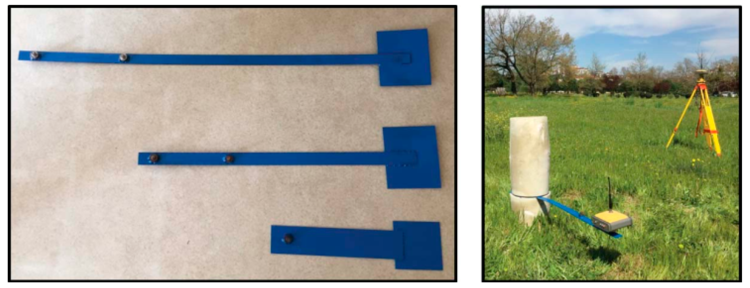
| Validation of performance of real-time kinematic PPP for deformation monitoring | Displacement monitoring test measured by telescopic pole | Martín et al. [60] | |
| PPP sliding window algorithm for deformation monitoring | Simulation data and earthquake data | Song et al. [61] | |
| Precise dynamic displacements detection | Field experiments | Different processing scenarios | Paziewski et al. [62] |
| High-rate PPP for detecting dynamic vertical displacement | ContT & RTK | Bar experiment | Yigit et al. [57,63] |
| PPP assessment of PPP accuracy for displacement waveforms | Acc & RTK | Experiment based on oscillator | Moschas et al. [64] |
| Epoch-wise station displacement | GPS seismology | Rapture model | Shi et al. [65] |
| Response analyses of Greece’s earthquake based on GNSS-PPP | GPS seismology | Frequency domain analysis | Kaloop et al. [66] |
| Aim | Experimental Scene | Application Domain | Method | Verification Scheme | Literature |
|---|---|---|---|---|---|
| Real-time GPS seismology with a stand-alone receiver | Simulation data and real earthquake data | GPS seismology | VADASE | Colosimo et al. [67] | |
| Exploiting the VADASE algorithm | Earthquake data of GPS and accelerometer | Accelerometer | Benedetti et al. [68] | ||
| Near real-time, tsunami early warning system | Earthquake data from IGS sites | PPP and differential positioning | Branzanti et al. [69] | ||
| High-rate multi-GNSS observations for real-time capture of seismic waves | GPS and BDS data of an earthquake | Postprocessed GPS PPP and strong motion data | Geng et al. [71] | ||
| Performance evaluation of VADASE using very high-rate GPS | Moderate and large earthquakes | Postprocessed GPS PPP | Shu et al. [72] | ||
| GPS seismology for a moderate magnitude earthquake | High-rate GPS data of an earthquake | PPP, differential positioning, VADASE | Strong motion accelerometer | Hung et al. [70] | |
| VADASE enhancement | GPS data of an earthquake | Improved VADASE | PPP | Fratarcangeli et al. [73] | |
| VADASE onboard a stand-alone GNSS receiver | Static tests and controlled dynamic tests | Structural monitoring | VADASE | ASHCROFT et al. [74] | |
| Different low-cost sensors for small amplitude oscillatory motion monitoring | One-direction vibrating table | High-speed, high-resolution camera | Benedetti et al. [76] |
| VADASE | PRM | SPM | |
|---|---|---|---|
| Need reference station | No | Yes | Yes |
| GNSS receiver type | Single frequency Multi-frequency Multi-GNSS | Single frequency Multi-frequency Multi-GNSS | Single frequency Multi-frequency Multi-GNSS |
| Receiver sampling frequency requirement | High-rate | High-rate | High-rate |
| observations | Carrier phase | Double-differenced phase | Double-differenced phase |
| Principle | Difference between epochs | Select the phase residuals of two special satellites | Difference between epochs |
| Number of satellites | At least four common satellites in consecutive epochs | Two satellites in two special directions | At least four common satellites in consecutive epochs |
| Denoising or detrending | Yes | Yes | Yes |
| Aim | Experimental Scene | Verification Scheme | Measurement Method | Literature |
|---|---|---|---|---|
| Single frequency GPS deformation monitoring | A bridge deformation monitoring network with four stations and another more complicated network in the southwest of USA | Single frequency RTK | Huang et al. [83] | |
| Verify the feasibility of using single-frequency GPS-RTK for bridge deformation and vibration monitoring. | Zero baseline trials and field bridge trials | Dual frequency RTK | Cosser et al. [87] | |
| Real-time PPP method of single frequency receiver based on CORS network | CORS network in Shanxi Province and Hubei Province, China | Dual frequency positioning result calculated by using GAMIT | Jiang et al. [84] | |
| Verify the feasibility of single-frequency PPP-RTK | GPS Network Perth in Australia | The high-grade dual-frequency positioning result | Single-frequency PPP-RTK | Odijk et al. [85] |
| Method | Pos mea | Ref stat | Research status | Pros | Cons | |
|---|---|---|---|---|---|---|
| RTK | RTK | ✓ | ✓ | Applications [25,26,27,47,48] | Mature technology | Limited coverage The problem that the reference station is also in the deformation area |
| Network RTK | Early-stage research [43] | Wide coverage Reliable | Needs service providers | |||
| Single frequency RTK | Research [83,87] | Low-cost | Needs ionospheric corrections from reference stations | |||
| PPP | PPP | ✓ | ✕ | Applications [56,66] | No reference station required | Real-time data stream is needed Long initialization time |
| Single frequency PPP | Research [84,85] | Low-cost | ||||
| GNSS & Accelerometer | ✓ | Applications [32,45,89,90,91,92,93] | Robust Complementary advantages | Data processing is relatively complex | ||
| Displacement Measurement | VADASE | ✕ | ✕ | Applications [67,68,69,70,71,72,73,74,75,94] | The integration of multi-GNSS systems is easier | Absence of absolute position, drifts |
| PRM | ✓ | Applications [77,78,79,80,81,82,95] | ||||
| SPM | ✓ | Research [62] | ||||
| Aim | Sample Rate | Method | Experimental Scene | Verification Scheme | Literature |
|---|---|---|---|---|---|
| Noise characteristics of short-duration, GPS-records | 10 Hz | Correlation analysis and spectral analysis of displacement time-series | Static observation | Moschasa et al. [114,119] | |
| Noise characteristics and implications for monitoring networks | 2–50 Hz | RTK | Genrich et al. [118] | ||
| PLL bandwidth and noise in GPS measurements | 100 Hz | Correlation analysis and spectral analysis of displacement time-series | Moschas et al. [113] | ||
| Epoch-wise station displacement | 1 Hz | PPP | GPS seismology | Rapture model | Shi et al. [65] |
| Broadband displacements | 1 Hz | Loose integration | Acc | Bock et al. [90] | |
| Evaluation of the variometric approach | 1 Hz, 50 Hz | VADASE | PPP | Shu et al. [72] | |
| Assessment of high-rate GPS for seismology | 100 Hz | Correlation analysis of position | Shake table | ContT | Häberling et al. [117] |
| High-rate PPP for detecting dynamic vertical displacement | 10 Hz | PPP | Bar experiment | ContT & RTK | Yigit et al. [57] |
| Precise dynamic displacements detection | 50 Hz | PPP, RTK, SPM | Static observation | Paziewski et al. [62] | |
| Measure seismic wave motions | 10–50 Hz | PPP | GPS data and IMU data from shake table | IMU | Xu et al. [56] |
| Assessment of PPP accuracy for displacement waveforms | 10 Hz | PPP | Experiment based on oscillator | Acc & DGPS | Moschas et al. [64] |
| Structural deflection monitoring | 10 Hz, 50 Hz | RTK | Bridge | Acc | Roberts et al. [29] |
| Assessment of high-rate GPS receivers for deformation monitoring of bridges | 50 Hz, 100 Hz | RTK | Bridge | Acc, FEM | Yi et al. [115] |
| Experimental Scene | Fusion Method | Detail | Limitations | Literature |
|---|---|---|---|---|
| Bridge monitoring | AF | Acceleration aided the AF approach to isolate relative movements of the bridge | Detectable frequency is limited by the original GPS | Meng. [32] |
| Motion simulation table tests and super high-rise building monitoring data | Method based on AF and EMD | Enhanced the measurement of static and dynamic accuracy | Algorithm implementation is complicated | Chan et al. [93] |
| Dynamic displacement of steel pedestrian footbridge | A multi-step filtering procedure | Accelerometer was used to constrain and assess the filtering procedure | Accelerometer information is not fully utilized | Moschas et al. [45] |
| Aim | Experimental Scene | State Variables | Measurement | Literature |
|---|---|---|---|---|
| Multi-rate Kalman filtering for the data fusion | Simulation | Displacement and velocity | Displacement from GPS measurement | Smyth et al. [92] |
| Providing a broadband record of ground displacements | Shake table experiments and earthquake data | Bock et al. [90] | ||
| Load response on a large suspension bridge by GPS and accelerometers | A highway suspension bridge excited by marathon runners | Kogan et al. [91] | ||
| Low-cost RTK-GPS sensor and a force feedback accelerometer for infrastructure monitoring | Lab-scale vibration tests and field suspension bridge tests with a passing train | Displacement, velocity and acceleration | Displacement measurements from RTK-GPS | Koo et al. [89] |
| Aim | Experimental Scene | Roles | Literature |
|---|---|---|---|
| GPS–accelerometer data integration for deformation monitoring | Motion simulation table tests | Decomposing the time history of GPS for final residuals. Decomposing the accelerator-measured dynamic displacement time history to extract high-frequency components. | Chan et al. [93] |
| Analysis and denoising of GPS Data | Simulation data and field GPS data | Denoising the white and colored noise | Baykut et al. [170] |
| Mine surveying of complex field conditions | field GPS/PLs data | Extracting the un-modeled systematic errors | Chao et al. [149] |
| Deformation monitoring based on the GPS/Pseudolites technology in open-pit mine | Simulation data and field GPS/PLs data | Jianpeng et al. [157] | |
| Mining subsidence monitoring | Field GPS RTK | Chao et al. [155] | |
| Reducing GPS carrier phase errors for precise static positioning | Field GPS data | Wang et al. [150] | |
| GPS multipath effect Mitigation | A calibration test | Mitigating multipath effect | Chen et al. [166] |
| Multipath mitigation for GPS dynamic deformation monitoring | Simulation data and field GPS data | Dai et al. [167] | |
| Assessing methods of RTK-GPS/accelerometer integration to monitor the displacement of structures | Field test data with reference from another sensor | Filtering of the acceleration data | Hwang et al. [168] |
| Extracting white noise statistics in GPS coordinate time series | Both simulated GPS coordinate time series and real data | Extracting White Noise Statistics | Montillet et al. [169] |
| Denoising GPS-based Structure monitoring data | Simulation data and field GPS data | Decomposing displacement for further processing | Ke. [151] |
© 2019 by the authors. Licensee MDPI, Basel, Switzerland. This article is an open access article distributed under the terms and conditions of the Creative Commons Attribution (CC BY) license (http://creativecommons.org/licenses/by/4.0/).
Share and Cite
Shen, N.; Chen, L.; Liu, J.; Wang, L.; Tao, T.; Wu, D.; Chen, R. A Review of Global Navigation Satellite System (GNSS)-Based Dynamic Monitoring Technologies for Structural Health Monitoring. Remote Sens. 2019, 11, 1001. https://doi.org/10.3390/rs11091001
Shen N, Chen L, Liu J, Wang L, Tao T, Wu D, Chen R. A Review of Global Navigation Satellite System (GNSS)-Based Dynamic Monitoring Technologies for Structural Health Monitoring. Remote Sensing. 2019; 11(9):1001. https://doi.org/10.3390/rs11091001
Chicago/Turabian StyleShen, Nan, Liang Chen, Jingbin Liu, Lei Wang, Tingye Tao, Dewen Wu, and Ruizhi Chen. 2019. "A Review of Global Navigation Satellite System (GNSS)-Based Dynamic Monitoring Technologies for Structural Health Monitoring" Remote Sensing 11, no. 9: 1001. https://doi.org/10.3390/rs11091001