UAV Multispectral Imagery Combined with the FAO-56 Dual Approach for Maize Evapotranspiration Mapping in the North China Plain

1
College of Water Resources and Architectural Engineering, Northwest A&F University, Yangling 712100, China
2
Key Laboratory of Agricultural Soil and Water Engineering in Arid and Semiarid Areas, Ministry of Education, Northwest A&F University, Yangling 712100, China
3
Institute of Soil and Water Conservation, Northwest A&F University, Yangling 712100, China
4
College of Mechanical and Electronic Engineering, Northwest A&F University, Yangling 712100, China
*
Author to whom correspondence should be addressed.
Remote Sens. 2019, 11(21), 2519; https://doi.org/10.3390/rs11212519
Submission received: 3 September 2019
/
Revised: 21 October 2019
/
Accepted: 23 October 2019
/
Published: 28 October 2019
(This article belongs to the Section Remote Sensing in Agriculture and Vegetation)
Abstract
:As the key principle of precision farming, variation of actual crop evapotranspiration (ET) within the field serves as the basis for crop management. Although the estimation of evapotranspiration has achieved great progress through the combination of different remote sensing data and the FAO-56 crop coefficient (Kc) method, lack of the accurate crop water stress coefficient (Ks) at different space–time scales still hinder its operational application to farmer practices. This work aims to explore the potential of multispectral images taken from unmanned aerial vehicles (UAVs) for estimating the temporal and spatial variability of Ks under the water stress condition and mapping the variability of field maize ET combined with the FAO-56 Kc model. To search for an optimal estimation method, the performance of several models was compared including models based on Ks either derived from the crop water stress index (CWSI) or calculated by the canopy temperature ratio (Tc ratio), and combined with the basal crop coefficient (Kcb) based on the normalized difference vegetation index (NDVI). Compared with the Ks derived from the Tc ratio, the CWSI-based Ks responded well to water stress and had strong applicability and convenience. The results of the comparison show that ET derived from the Ks-CWSI had a higher correlation with the modified FAO-56 method, with an R2 = 0.81, root mean square error (RMSE) = 0.95 mm/d, and d = 0.94. In contrast, ET derived from the Ks-Tc ratio had a relatively lower correlation with an R2 = 0.68 and RMSE = 1.25 mm/d. To obtain the evapotranspiration status of the whole maize field and formulate reasonable irrigation schedules, the CWSI obtained by a handheld infrared thermometer was inverted by the renormalized difference vegetation index (RDVI) and the transformed chlorophyll absorption in reflectance index (TCARI). Then, the whole map of Ks can be derived from the VIs by the relationship between CWSI and Ks and can be taken as the basic input for ET estimation at the field scale. The final ET results based on multispectral UAV interpolation measurements can well reflect the crop ET status under different irrigation levels, and greatly help to improve irrigation scheduling through more precise management of deficit irrigation.

1. Introduction
In semiarid regions, the climate is characterized by long periods of drought and strong interannual variability in rainfall amounts and distribution, leading to high year-to-year variability in agricultural development and production [1]. The North China Plain is one of the most important agricultural regions because it accounts for about one-fifth of national food production. In this area, rainfall cannot meet the crop water requirements, and the overexploitation of groundwater aggravates water scarcity, reduces the groundwater table, and threatens sustainable agriculture [2]. Irrigation is then necessary to prevent water stress and ensure profitable yields. To determine the optimal irrigation scheduling and adopt such strategies efficiently, it is necessary to have reliable methods of providing information about the temporal and spatial variability of crop evapotranspiration (ET) within the field scale [3].
The direct ET measured methods consist of the use of a lysimeter, eddy covariance, Bowen ratio, and soil water balance. However, they face important limitations due to expensive techniques and low spatial representativeness of measurements, particularly in agricultural fields characterized by a high level of heterogeneity in terms of crops and water status [4]. The indirect form can be made from empirical equations that use agronomic, biophysical, and meteorological elements as input variables [5]. As the most widely used method for the determination of ET, the FAO-56 dual crop coefficient (Kc) approach, published by the Food and Agriculture Organization in Irrigation and Drainage Paper No. 56 [6], has received favorable acceptance and application worldwide [5,7]. The dual Kc approach describes the relationship between the daily evapotranspiration of a given crop and the reference evapotranspiration (ET0) by separating the single crop coefficient into the basal crop coefficient (Kcb), soil water evaporation (Ke) coefficient, and water stress coefficient (Ks). Although simple in design and construction, the dual Kc method successfully incorporates a number of consistent and compensating factors that distinguishes the ET of any unique crop from that of the reference ET [7]. However, the method is mainly used for the ET estimation based on stationary measurements and cannot provide a fine estimation due to inconsistent crop growth.
To explore the distribution of crop ET within the field scale, remote sensing technology provides a dependable basis [8]. The crop coefficient generated from remote sensing based on canopy reflectance responds to the actual crop condition, captures the variability among different local atmosphere conditions and field spatial variability [9], and reflects the heterogeneity of plant development in large irrigated fields [10,11,12,13,14]. Studies have established different inversion models between vegetation indices (VIs) and Kcb [15,16,17,18]. For decades, satellite remote sensing images have been the main data sources to integrate the FAO-56 for the estimation of crop ET. For example, Bellvert et al. [19] used a dataset of the vegetation index (NDVI) derived from Landsat-8 to facilitate the estimation of the Kcb, and potential crop water use. However, the low spatial and temporal resolution of satellite data limits its further application in estimating ET within the field scale. At the same time, cloud cover remains a significant challenge in satellite-based remote sensing [20].
As one of the most important emerging remote-sensing platforms, unmanned aerial vehicles (UAVs) have been gradually employed in precise agriculture. Soon, UAVs will be vital tools for growers as they can cover large areas, and take advantage of new sensing, mapping, and data analytical technologies [21,22,23]. Real time mapping and rapid image analysis also provide the early detection of plant water status for timely irrigation scheduling [24]. Based on these advantages, UAVs have broad application prospects for more sophisticated ET management within the field scale. When dealing with the estimation of ET based on a combination of UAV and the dual Kc method under water stress conditions, four parameters are required: ET0, Kcb, Ke, and Ks. ET0 can be estimated using the FAO Penman–Monteith formula and the collected meteorological data [25]. Ke is clearly correlated with foliage cover and irrigation/rainfall event, and becomes negligible when the crop completely covers the soil [26]. Many studies have validated that Kcb has a strong correlation with NDVI and foliage cover, and applied to practical water requirement monitoring [16,27]. For instance, Han et al. [28] studied the feasibility of UAV multispectral remote sensing in the estimation of maize crop coefficients at different growth stages. The results showed a strong relationship between UAV-measured NDVI and Kcb, with an R2 value of 0.82. Although the assimilation of FAO-56 and remote sensing data has made such great progress, discrepancies between the measured and simulated ET remained when water stress occurred.
The accurate estimation of Ks is the key to accurately estimate crop ET using UAV remote sensing data under water stress conditions. Specifically, Ks represents the fraction of potential transpiration rate, with a value from 1 to 0, according to the level of water stress, which is directly related to the water content in the root zone. Less attention has been paid on determining the water stress coefficient Ks from the remote sensing data because there are difficulties in estimating soil and root zone moisture (or root zone depletion) from remote sensing data [29]. It is necessary to use a new indictor, which is easy to obtain and can respond to real-time plant-water status. Studies [30,31] have proven that canopy temperature (Tc) is closely related to soil water content, actual transpiration, and crop water stress status. Therefore, Ks and canopy temperature are definitely related to each other. Olivera et al. [32] used the vegetation and soil temperatures retrieved from LST (land surface temperature) data derived from the eddy covariance system to estimate the Ks. This method is based on the polygon defined in the LST–VI space, which needs a large amount of temperature data and has a complex analysis procedure. Recently, studies have evaluated indices based on Tc that require less information for detecting crop water stress and have shown that Ks is related to several crop water stress indices. For instance, Bausch et al. [18] successfully used a ratio of canopy temperature as a substitute for the soil moisture based Ks. The ET difference between the two deficit irrigation treatments for the 25-day investigative period calculated by Tc ratio and water balance techniques was 21 mm and 4 mm. Kullberg et al. [33] observed that using an appropriate Ks method had the potential to improve irrigation scheduling to properly manage stress and ensure optimum crop yield under a limited irrigation water supply. A noted advantage of non-dimensional crop indices such as CWSI (crop water stress index) is that they are typically considered to be scalable to Ks for ET estimation (i.e., Ks = 1 − CWSI). This is also the basis behind the Tc ratio approach, although it has dimensionality restrictions [34]. For the estimation of Ks based on water stress indices, most studies have used handled or stationary infrared thermometers [33,34,35]. A ground-based platform is still time consuming and labor intensive. Additionally, like the estimation by counting root zone depletion, it is impractical to estimate ET by combining the Kcb of large image pixels with Ks based on ground-point measurements due to the heterogeneities of the crop and soil status.
With the development of agricultural technology, high-resolution thermal imagery acquired by UAVs has been used to map plant water stress indices such as the CWSI, and water deficit index (WDI). However, when Kcb and Ks are obtained from different sensors (i.e., multispectral and thermal sensors), the problem of data fusion and matching will be obstacles to ET estimation with the UAV system. For example, as the image resolution obtained by the two sensors is different, image matching with different resolutions requires a complicated process. Most importantly, the biggest effect is not only on the pixel mixing due to the downscale, but on the georectification and co-registration of the images, therefore, the asynchronous time and space of the Ks and Kcb may influence the acquisition of maize ET. Previous studies have indicated that multispectral VIs have significantly high correlation with water stress indicators. For example, Samuel et al. [36] summarized the common spectral vegetation indices (VIs) that have been correlated to plant water stress. Studies [37,38,39] suggested that the renormalized difference vegetation index (RDVI) and transformed chlorophyll absorption in reflectance index (TCARI) are useful in plant stress monitoring. Therefore, the synchronized acquisition of Kcb and Ks using one sensor (i.e., a multispectral camera) should be explored.
This study aimed to estimate more accurate ET maps with UAV-based multispectral images over maize in the semiarid region of the North China Plain by applying the FAO-56 dual Kc approach. More specifically, we first compared the ET derived from water stress indices (CWSI and Tc ratio) and NDVI to that calculated with the modified FAO-56 dual Kc method by evaluating the suitable water stress indicator for local maize ET estimation. Next, we investigated the potential of assimilating ET estimation with VIs data (multispectral UAV) through the retrieve relation between the water stress index and VIs to eliminate discrepancies caused by using data at different scales and obtain a high resolution (4.7 cm) spatial-temporal ET map.
2. Materials and Methods
2.1. Study Site and Experimental Design
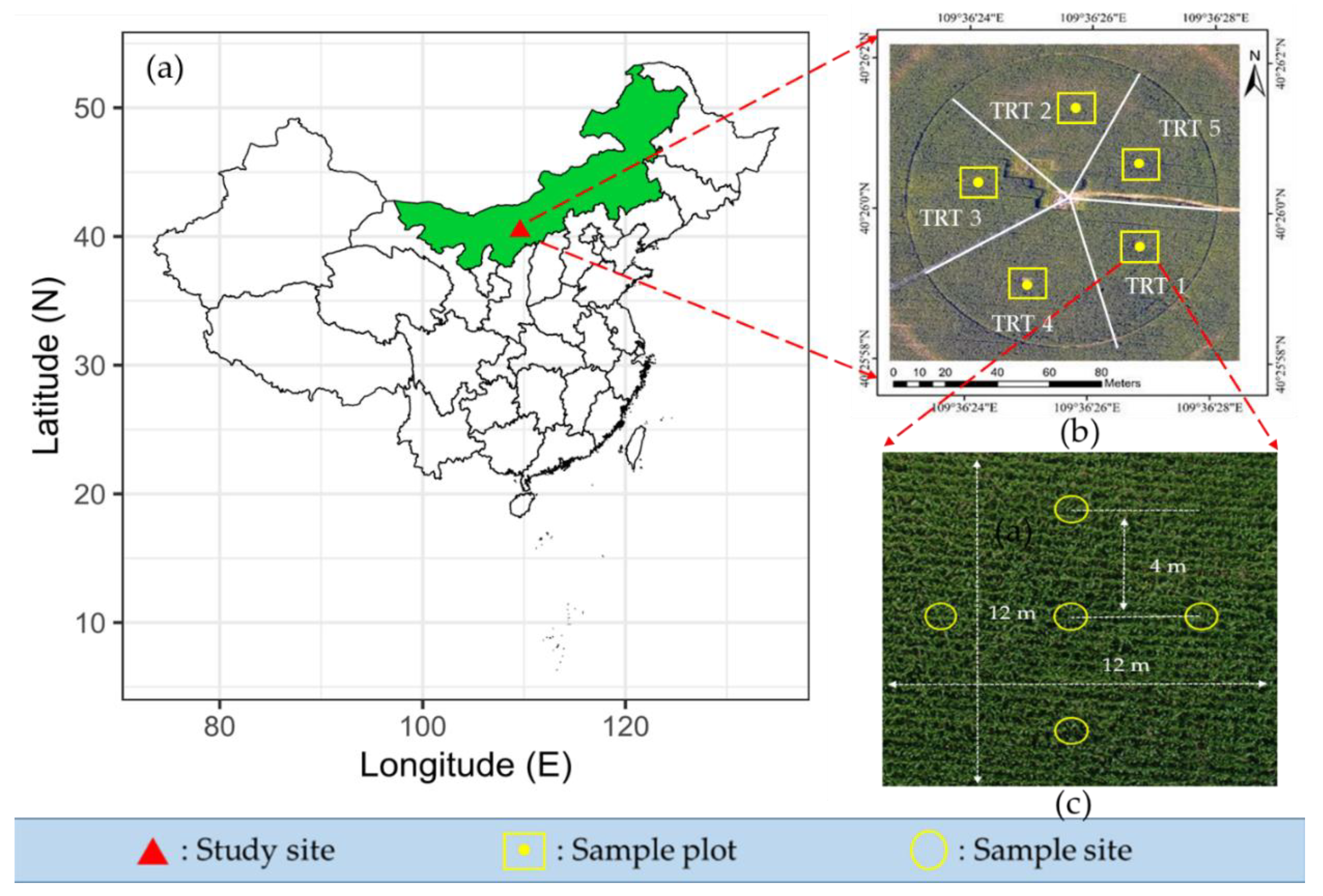
A 1.13 ha research field located in Zhaojun Town, Dalate Banner, Ordos, Inner Mongolia, China (40°26’0.29”N, 109°36’25.99”E, Elev. 1010 m; Figure 1a) was chosen to conduct the study. Maize (Junkai 918) was planted on 20 May 2017 with a 0.58 m row spacing and 0.25 m plant spacing, and the row direction was east–west. The maize emerged on 1 June, headed on 20 July, and was harvested on 7 September (silage), with a 110-day lifespan.
The study field was divided into five treatment (TRT) zones (Figure 1b) with three different levels of irrigation at the vegetative, reproductive, and maturation growth stages. Each treatment zone had one sample plot (Figure 1b), and each sample plot had five sample sites (Figure 1c). The five water treatments are given in Table 1. The total crop water requirement of the full watered maize field during the late vegetative, reproductive, and maturation stages was 407 mm, which was close to the total applied water (402 mm) of the control treatment zone (TRT 1). Water for other TRTs was applied proportionally to that for TRT 1. Since TRTs 1, 2, and 3 represented the three levels of irrigation, only these zones were taken for the analysis. Irrigation water was applied during the growing season by using a centered pivot irrigation system (Valmont Industries Inc., USA), with the coefficient of uniformity of the first span (research field) of 82.7% with a speed of 20%, or at 88.3% with a speed of 40%, as calculated by the modified formula of Heermann and Hein [40] by using R3000 sprinklers. The amount of water applied to each treatment was measured and recorded by MIK-2000H flow meters (Meacon Automation Technology Co. Ltd., Hangzhou, China), and the accuracy of the flow meters was better than 1%. The actual amount of irrigation and rainfall at each growth stage are shown in Table 1. The soil type is a loamy sand according to the soil taxonomy of the United States Department of Agriculture. More detailed information about the soil characteristics are listed in Table 2. To eliminate the interference of nutritional stress and weeds, fertilizer and herbicide were applied according to the planting experience.
2.2. Framework and Parameters for Assimilating Remote Sensing Data into FAO-56 Crop Coefficient Method
Figure 2 shows the assimilation of remote sensing data into the FAO-56 dual crop coefficient method for the estimation of evapotranspiration in this study. Unlike the traditional FAO-56 single crop coefficient method, canopy reflectance was used to reflect crop growth and water stress, and then the dual crop coefficient was obtained based on the UAV-measured spectral data. Finally, point-scale evapotranspiration was extended to the whole field through the UAV multispectral images under different irrigation levels. Table 2 shows the soil characteristics and parameters used in the modified FAO-56 dual crop coefficient assimilation procedure for maize.
2.2.1. Meteorological Factors and Soil Water Content
The weather data were obtained from an automated weather station located on a grass reference surface (0.95 ha) that was 1000 meters away from the research field, with observations of rainfall, air temperature (Ta), humidity, net solar radiation (Rn), and wind speed (2 m above the reference surface). Except for rainfall, the data acquisition interval was 30 minutes.
Soil water content (SWC) was measured two or three times each week on the day before or after irrigation within each sampling plot by the traditional gravimetric method [43]. At each sampling plot, three sampling sites were randomly chosen around the center. The samples were collected by soil augers at depths of 30 cm, 60 cm, 90 cm, and 120 cm. Soil samples were put in aluminum boxes to avoid the influence of evaporation. Basically, the gravimetric method involves taking soil samples, weighing, oven-drying, and reweighing them, then expressing the moisture content (i.e., loss in weight) as a percentage of the oven-dry weight. This is the weight or mass basis of expressing soil moisture content. Then, by multiplying the bulk density, the results can be expressed in terms of volume [44]. The average SWC (θ) was estimated by interpolating the soil moisture observations of the different depths belonging to the root-zone of maize.
2.2.2. Measurement of Maize Parameters
Maize canopy temperature (Tc) and UAV multispectral data were synchronously collected under clear sky at solar noon. Tc was collected during the full foliage cover period (6–29 August 2017 including the reproductive and maturation stages). A handheld infrared thermometer (Raytek ST60+, Raytek Inc., Santa Cruz, CA, USA) was used to measure Tc with a measurement error of ±1 °C or ±1% of the reading. The larger values were adopted in the practical application. The temperature and spectral ranges of the Raytek ST60+ are −32–600 °C and 8–14 μm, respectively. The emissivity value was set to 0.97 [45]. To avoid the interference of soil, the thermometer was used to sweep the canopy (about 120°) perpendicular to the row, 30 cm above the canopy, and at a 15° horizontal angle. At each sample site, three measurements were made to obtain the Tc. The values averaged over one sampling site or over one plot (yellow circle in Figure 1c) were taken to represent their status.
The main plant parameters needed to run the modified FAO-56 model (see Section 2.2.3) are canopy height (h) and leaf area index (LAI). A random sampling method was used to collect the LAI and plant height of maize. An LAI-2200C canopy analyzer (LI-COR Biosciences, Lincoln, NE, USA) was used to measure the LAI of maize; 10 sampling points were randomly selected for each plot and the average value was obtained. For each plot plant height of maize, 15 representative maize plants were randomly selected and measured by tape measure. Cubic spline interpolation is a piecewise regression approach that uses third-order polynomials for interpolation between a series of paired data points [14]. Thus, cubic spline was used to process the measured LAI and plant height data, and then the daily sequence of maize LAI and plant height data were obtained.
2.2.3. The Modified FAO-56 Dual Crop Coefficient Method
In FAO-56, the actual ET is defined as the product of crop coefficient (Kc) and reference evapotranspiration (ET0) [26]. In the dual Kc model, Kc is split into two factors that separately describe the evaporation (Ke) and transpiration (Kcb) components. The method has been widely used in scheduling irrigation and improving agricultural production [46]. FAO-56 ET is estimated as follows:
where ET is in mm/d; Ke is the evaporation coefficient of the bare soil fraction; Kcb is the basal crop coefficient; Ks is the water stress coefficient; and ET0 is the grass reference evapotranspiration in mm/d. The stages of canopy temperature acquisition and ET estimation were in the period of high coverage (i.e., vegetation cover ranging from 0.79 to 0.84 as estimated by an empirical equation based on NDVI [47]). With Ke = 0.25 × (1 − fc) [26], it had a minor influence on total ET and was ignored.
The ET0 of this reference surface was estimated according to the following Penman–Monteith equation:
where Rn is the net radiation at the crop surface; G is the soil heat flux density (as the magnitude of the 1-day or 10-day soil heat flux beneath the grass reference surface is relatively small, it may be ignored, thus Gday = 0 [26]); T is the mean daily air temperature at 2 m height; u2 is the wind speed at 2 m height; es is the saturation vapor pressure; ea is the actual vapor pressure; ∆ is the slope vapor pressure curve; and γ is a psychrometric constant.
The basal crop coefficient, Kcb, is generally obtained from the guidelines of FAO-56 by looking-up the tabulated value at every growth stage and then linearly interpolating it to obtain the daily values. The approach from the original FAO-56 dual Kc procedures cannot calculate the daily actual value of Kcb [42]. Feng et al. [48] modified Kcb with LAI through eddy covariance systems near the experimentation site, which illustrated that the modified dual crop coefficient method could estimate maize ET accurately on the North China Plain. Therefore, in order to evaluate the dynamic changes of ET in the maize field more accurately, the canopy height and LAI were used to modify the dynamic Kcb. The modified FAO-56 Kcb value can be calculated by Equations (3) and (4):
where Kc,min is the minimum for bare soil (0.15); Kcb,full is the estimated basal Kcb for vegetation having full ground cover; Kc,max is the maximum Kc (1.2); RHmin is the minimum relative humidity (%); and k is the canopy attenuation coefficient of radiation, and the value of k is listed in Table 2.
The crop water stress coefficient Ks related to the actual root zone water content is a key parameter for calculating and simulating soil water conditions. Several linear and curvilinear functions have been proposed to adjust for the effects of decreasing available water on ET or for the Ks used in Equation (1). The simple linear model for estimating Ks as described in FAO-33 is commonly used and calculated by Equation (5) ,which is an equivalent expression to the FAO-56 Ks procedure [49].
where θ is the mean volumetric soil water in the crop root zone and θj is the threshold water content, where transpiration decreases linearly due to water stress. Ks = 1 for θ ≥ θj. p is the fraction of available soil water that can be deleted from the root zone before moisture stress. The θfc is the field capacity, and θwp is the permanent wilting point. All θ (m3 m−3) represent averages over the effective root zone (Zr). The rooting depth Zr (m) is assumed to vary between a minimum value (maintained during the initial crop growth stage at 0.1 m) and a maximum value (that reached 1 m at the beginning of the mid-season stage). The maximum value was measured in the field and was equal to 1 m, according to FAO-56 [6]. When the θ was lower than θj, the crop begins to reach the stress period (Ks < 1), and if θ is less than θwp, the crop does not absorb water from the root zone (Ks = 0). Values for Equations (5) and (6) are listed in Table 2.
2.2.4. UAV (Unmanned Aerial Vehicle) Multispectral System, Data Collection, and VI (Vegetation Index) Calculation
In this study, a hexacopter UAV multispectral remote sensing system (Figure 3) was developed with a Pixhawk autopilot (CUAV, Guangzhou, China), a RedEdge multispectral camera (MicaSense, Inc., USA), and a MOY brushless gimbal (Moyouzhijia, Huizhou, China). Its maximum load was 5 kg, and the maximum flight duration was 30 minutes. The RedEdge multispectral camera has a focal length of 5.5 mm, a field-of-view angle of 47.2°, and an image resolution of 1280 × 960 pixels. The bandwidths and central wavelengths for the 5-band RedEdge are 20 nm at 475 nm (blue), 20 nm at 560 nm (green), 10 nm at 668 nm (red), 10 nm at 717 nm (red edge), and 40 nm at 840 nm (near infrared). The camera was equipped with a light intensity sensor and two 3 m × 3 m gray plates (Group 8 Technology, Provo, UT, USA). The light intensity sensor can correct the influence of external light changes on spectral images during aerial photography. The gray plate has fixed reflectivity; it can correct the reflectivity of multispectral images, generate reflectivity images, and extract the VI. The multispectral images of the gray plate (reflectivity 58%) collected simultaneously at the same height were used to perform radiometric correction. In Pix4DMapper a vignetting polynomial was used for radiometric correction. Then, the spectral reflectance of the objects was obtained. Flight planning was conducted with Mission Planner ground control station software, which allows the user to generate a route of waypoints as a function of the sensor field of view (FOV), the degree of overlap between images, and the ground resolution needed.
During the study period (20 June to 29 August 2017), 11 UAV flights were conducted on sunny days between 11:00 and 13:00 local time (Chinese standard time, 11:44–13:44) with the RedEdge camera lens vertically downward, and an 80% heading and side overlap. The flight height, speed, and pixel resolution were 70 m (relative flying height), 5 m/s, and 4.7 cm, respectively. A total of 2185 images (five bands) were collected during a single flight and Pix4DMapper software was used for image mosaicking.
To establish the regression models between UAV-based multispectral VIs and crop coefficients (NDVI vs. Kcb and TRCAI/RDVI vs. Ks), three VIs were selected: NDVI [50], transformed chlorophyll absorption in reflectance index (TCARI) [51], and the renormalized difference vegetation index (RDVI) [52]. In addition, cubic spline interpolation was used to determine the VI values between two flight overpasses. Their calculation equations are as follows:
where ρnir, ρred, ρrededge, and ρgreen are the reflectance values of ground objects in the near-infrared, red, red-edge, and green bands, respectively.
2.2.5. Crop Coefficient Estimation Using Reflectance Data
Reflectance-based basal crop coefficient (Kcb) methods have been used to improve the irrigation scheduling of maize. NDVI is one of the most widely used indices for estimating crop parameters. This index is highly sensitive to variations of LAI and the fraction of the ground that is covered by vegetation, (fc). The NDVI has a linear relationship with fc along the whole range of vegetation cover [47]. Accordingly in this study, Equation (10) was used for fc estimation. In this study, one 12 m × 12 m area was selected as the spectral sampling plot in each treatment (yellow box in Figure 1b). Studies [53,54] showed that Kcb can be estimated from fc.
where NDVImin and NDVImax are the minimum and the maximum values of the NDVI associated with bare soil and dense vegetation, respectively. Once fc has been obtained through Equation (10), the Kcb can be estimated as:
The two different Ks obtained from CWSI and Tc ratio were derived from the handheld infrared thermometer, with daily values taken around local times between 11:00 and 13:00 (local time), which are approximate times of peak stress.
Jackson et al. [30] showed that CWSI is inversely related to the water use of the crop under consideration; Ks can also be calculated from CWSI by:
One of the widely used methods for estimating CWSI is based on measured canopy temperature [30,55]. The CWSI is defined in Equation (13).
where dTm, dTLL, and dTUL are the actual measurement, lower limit, and upper limit of the canopy–air temperature difference (Tc−Ta), respectively. More detailed information about local CWSI measurements can be found in Zhang et al. [39]. CWSI = 0 indicates no water stress, while CWSI = 1 indicates the most severe stress.
Zhang et al. [39] established linear regression models (R2 = 0.80, p < 0.001) between TRCAI/RDVI and CWSI (Equation (14)). The local calibration of CWSI performed in [39] was also retained here. Thus, we could integrate the remote sensing data into the Ks model by establishing a stable relationship between VIs and CWSI. According to the relationship between Ks and CWSI (i.e., Ks = 1 − CWSI) and to rescale the Ks value between 0 and 1, the linear regression models can been shown as per Equation (15):
An alternative method to evaluate water stress that only requires the crop canopy temperature was proposed by Bausch et al. [35]. The relationship between Ks and Tc ratio is as follows:
where Tc ratio is a stress coefficient proposed as a surrogate for the water stress coefficient Ks from FAO-56. Tc is the canopy temperature and TcNS is the temperature of a fully irrigated, non-stressed canopy, which was chosen as the lowest canopy temperature observed at the given timestamp including all treatments [34]. This temperature ratio was found to be capable of quantitatively monitoring water stress and can potentially be used in the place of the water stress coefficient when soil water measurements are not available.
2.2.6. Evapotranspiration Comparison and Statistical Analysis
Due to the lack of validation information from an eddy covariance tower or lysimeter, the ET estimated by the modified dual Kc method [42,48] was used to validate the model. Ding et al. [42] found good agreement between the predicted ET and transpiration using the modified model and the measurements through the lysimeter for maize in 2010, with a slope of linear regression of 0.99 (R2 = 0.90) and 1.01 (R2 = 0.92). Feng et al. [48] also obtained similar results and suggested that the modified dual crop coefficient method was suitable for calculating the actual daily ET of the main crops across the North China Plain. Studies [56,57] also used the local ET estimated by the FAO-56 Kc method to validate the derived ET from their model. Thus, employing the ET data estimated by the modified FAO-56 dual Kc method as the validation set had certain accuracy in this study. The simulated daily ET of the maize derived from the two Ks methods and NDVI-based Kcb methods (ET-CWSI and ET-ratio) were compared with the values obtained from the modified FAO-56 dual crop coefficient method. The ET-CWSI, ET-ratio, and ET-FAO values were compared by using a linear regression analysis and the statistical parameters of the coefficient of determination (R2), root mean square error (RMSE), and index of agreement (d) were used as a relative measure of the difference among variables. Perfect agreement would exist between the observed and modeled values if d = 1.
Finally, we compared the cumulative evapotranspiration (CET) obtained by the VI method with the water balance approach to evaluate the ability of ET determination by UAV. Cumulative ET obtained by the soil–water balance [58] was used as the reference ET, and a relatively simple relation is expressed as:
where Pr is the effective precipitation; I is the irrigation depth; U is the ground water replenishment; RO is the runoff from the soil surface; and DP is the deep percolation of water moving out of the root zone. ΔSW is the change between the first and last measurements of soil water storage within the root zone. All terms are expressed in mm. As soil water content sensors buried at different depths in the field showed that the soil moisture at 1.2 m changed little during the study period and the terrain inclination was <5%, the U, RO, and DP were also considered as zero. Based on the soil–water balance (Equation (17)) and the above criteria, the CET was determined as follows:
3. Results
3.1. Meteorological Conditions and Maize Status
The temporal evolution of ET0, daily average air temperature (ATa), and canopy temperature (Tc) of three different treatments for different growth periods are shown in Figure 4. The ATa and other meteorological data for the ET0 calculation were obtained from an automatic weather station. Observations showed the three parameters decreased as the maize growth period progressed. Driven by the ATa, ET0 presented a similar pattern to ATa, which conformed to the standard Penman–Monteith equation. The highest ATa and ET0 reached 28 °C and 9.69 mm during the studied period. Although higher air temperatures may increase ET0, it can also influence Tc and affect crop transpiration when Tc exceeds the suitable canopy temperature for maize growth. The Tc of three different water treatments used for calculating the water stress index (CWSI and Tc ratio) showed a certain numeric gradient from 6 to 29 August 2017. Overall, Tc increased with the degree of water deficit. Average Tc of TRTs 1 (full irrigation), 2 (severe deficit irrigation), and 3 (light deficit irrigation) were 26.4 °C, 28.3 °C, and 26.5 °C, respectively. The highest Tc in TRT 2 reached 34 °C.
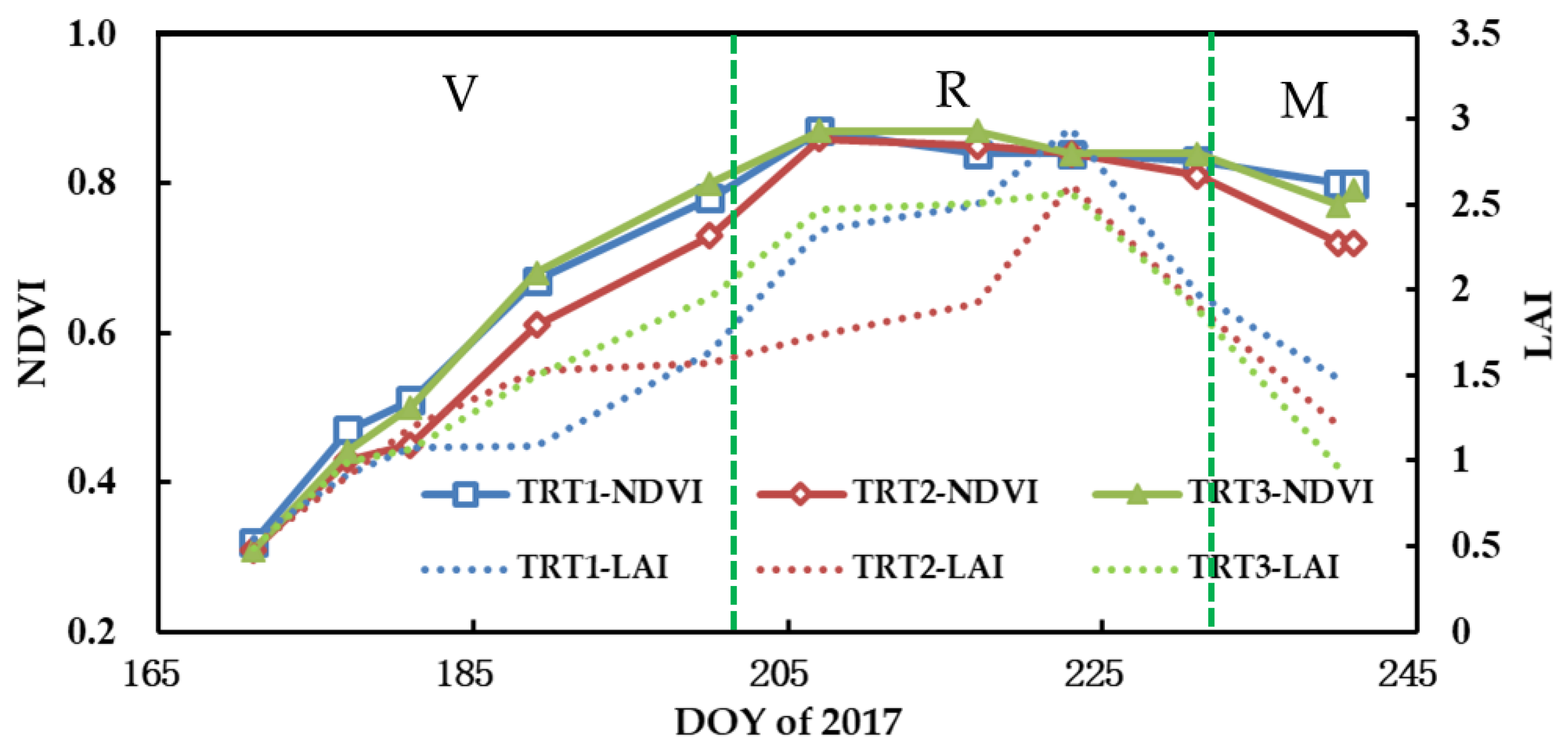
LAI is closely related to canopy structure, leaf number, and size, and has a strong effect on crop transpiration. When the crop is under water stress, leaf growth is affected (i.e., curl). Variation in the LAI can also influence canopy spectral information such as the NDVI. Figure 5 shows the changes of the NDVI and LAI from the vegetative to maturation stages (20 June to 29 August 2017) under three different irrigation treatments. The growth variables, NDVI and LAI, exhibited comparable seasonal patterns (i.e., first increased, and then decreased from early crop development to maturation). Due to the saturation of the NDVI, the maximum value of NDVI appeared faster than that of the LAI. The NDVI reached its maximum value of 0.84 in the late vegetative stage (DOY 207), while the LAI was still increasing up until the late reproductive stage (DOY 223). The average NDVI values for TRT 1, TRT 2, and TRT 3 were 0.69, 0.67, and 0.70 from the late vegetative to maturation stages, respectively, which was in line with the water stress levels. The NDVIs of TRT 1 and TRT 3 were approximately the same during the study stages, even though TRT 3 experienced light drought. The maximum difference between TRT 1 and TRT 3 was 0.03 on DOY 177. Furthermore, responses of different crop growth stages to crop water stress ere also different. The differences in the NDVI among the three treatments during the reproductive stage were smaller than those during the vegetative and maturation stages. For example, the differences between the NDVIs of TRT 1 and TRT 2 for the vegetation, reproductive, and maturation stages were 0.06, 0.01, and 0.08, respectively. The LAI patterns of the different treatments presented larger differences than those of the NDVI. Especially from the middle vegetative to middle reproductive stages, the maximum difference between the LAIs of TRT 2 and TRT 3 was 0.73 on DOY 207, illustrating that the LAI is more sensitive to water stress than the NDVI. On the other hand, the above facts show that it is not feasible to estimate ET only from the NDVI under water stress condition.
3.2. Kcb and Ks Calculated by Different Methosd
The basal crop coefficient, Kcb-Tab, calculated by the modified FAO-56 method (Equations (3) and (4)), was used to assess the capability of the reflectance-based basal coefficient model to provide accurate estimates of ET over the maize field under three treatments. According to the results computed by two methods in Figure 6, Kcb derived from UAV multispectral measurements closely tracked modified Kcb-Tab over the crop cycle and two Kcb responded well to the LAI (Figure 5) in different grown stages. They increased fast in the vegetative stage and then entered an asymptotic regime when the surface was almost covered by leaves (80%) in the reproductive stage. During the late reproductive stage, the Kcb values began to decline and the slope of the decrease in TRTs 2 and 3 were higher than TRT 1 due to the water stress. The Kcb-Tab and Kcb-NDVI in the three treatments also showed certain value differences. In general, the Kcb values increased with the irrigation levels. For instance, the average observed Kcb-NDVI were 0.86, 0.81, and 0.84 for TRT 1, 2, and 3, respectively.
Kcb only accounts for the potential evapotranspiration and the actual ET should be modified with Ks for crops undergoing deficit-irrigation. Two Ks obtained by the water stress indices CWSI and Tc ratio, which were calculated in turn by Tc, Ta, and Tc NS derived from the measurements of the handheld infrared thermometer, were used to evaluate the effects of water deficit on crop ET. Figure 7 shows the daily values of irrigation/rainfall events and different Ks values from various approaches for TRT 1 (Figure 7a), TRT 2 (Figure 7b), and TRT 3 (Figure 7c). The three Ks values increased after irrigation/rainfall and decreased with no irrigation/rainfall, responding well to irrigation/rainfall events. The Ks values for different levels of deficit irrigation in the reproductive and maturation stages had a clear numerical gradient. As TRT 1 was in the full irrigation area, the Ks calculated by the soil water content data (Equations (5) and (6)) was equal to 1, but a considerable part of the Ks calculated by the water stress indices was less than 1 (see Figure 7a). It is probable that even a well-watered crop could have a high canopy temperature because of very hot day. TRT 2 presented the lowest Ks values when compared with TRTs 1 and 3. The averaged Ks-CWSI, Ks-Tc ratio, and Ks-FAO were 0.94, 0.89, and 1 for TRT 1; 0.72, 0.81, and 0.66 for TRT 2; and 0.91, 0.88, and 0.88 for TRT 3 (see Table 3), respectively, indicating that TRTs 1 and 3 had less water stress than TRT 2. The daily changes of Ks calculated by different methods showed similar patterns, as depicted in Figure 7, while the sensitivity of different methods to water deficit was different, and the specific values between the three methods displayed relatively large differences in this study. On the whole, Ks-CWSI and Ks-FAO had greater variability than Ks-Tc ratio under water stress conditions, and the minimum Ks-FAO was as low as 0.38, while Ks-Tc ratio was 0.63 in the three treatments. Due to the drought resistance of crops, a reduction of water in the root zone does not immediately lead to crop stress. Thus, the canopy temperature may be a more realistic parameter than soil water content to represent the stress coefficient due to the complicated physiological processes that plants undergo as they encounter water stress and compensate for this stress.
3.3. Model Selection for Estimating Crop ET
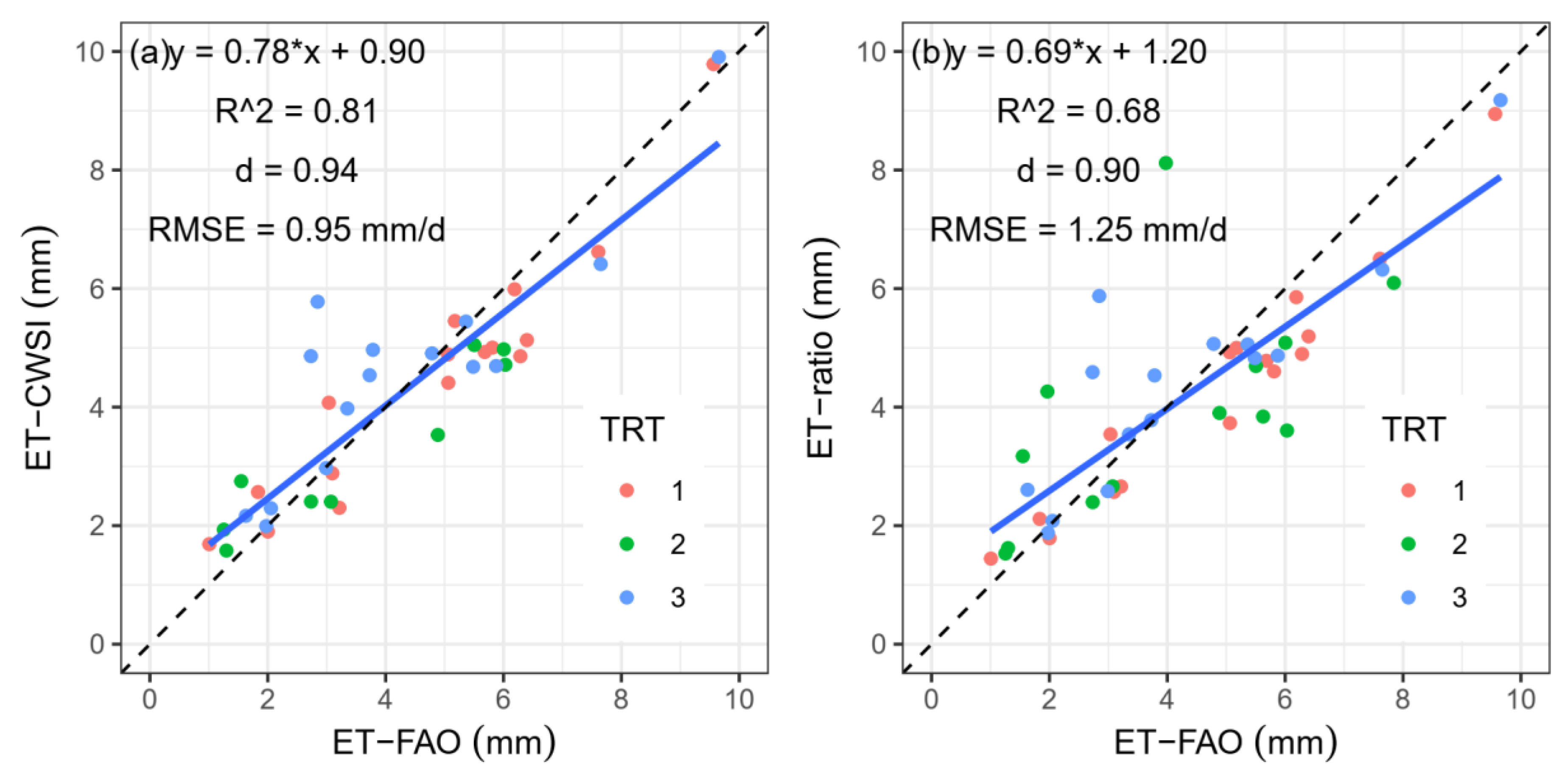
Maize ET for the three irrigation treatments during 6–29 August 2017 was calculated by various techniques. As the canopy temperature and soil water content (θ) acquisition were in the period of high coverage, and two or three days after the irrigation and precipitation. Thus, the minor influence of evaporation on total ET was ignored. The derived ET from the combination of two water stress indices and the combined NDVI-based Kcb (i.e., ET-CWSI and ET-ratio) were validated at the field scale using the modified FAO-56 ET (ET-FAO) by using three performance measure criteria (i.e., coefficient of determination (R2), root mean square error (RMSE), and index of agreement (d)). The value of d, which is presented in Figure 8a,b, was greater than 0.9 which indicates that ET based on water stress had a strong fit for the ET-FAO. However, ET-CWSI showed the least bias with an acceptable accuracy with an R2 = 0.81 and RMSE of about 0.95 mm/day (NRMSE = 11.1%), while the ET-ratio had an overall slightly lower correlation than the CWSI with a lower R2 = 0.68 and RMSE about 1.26 mm/day (NRMSE = 14.6%). Thus, the validation results from the R2 and RMSE viewpoints demonstrated that the CWSI method was better than the Tc ratio and could be used as a quantitative index to calculate maize evapotranspiration in this study.
3.4. Maize Evapotranspiration Maps Based on UAV Multispectral Remote Sensing Imagery
We retrieved the maize evapotranspiration map by combining the Ks map based on UAV TCARI/RDVI (Equation (15)) with the Kcb map based on the NDVI, according to the FAO-56 dual crop coefficient method. Figure 9 and Table 4 show the results of ET on DOY 217, 221, 231, and 241 during the reproductive and maturation stages. ET was seen to decrease with decreasing irrigation among the three different irrigation levels. On DOY 217, the highest value of ET in the study field reached approximately 8 mm because of the previous day’s rainfall. In addition, different treatments presented similar mean ET on DOY 217. On DOY 231 and 241, there were relatively less ET because of higher temperature and less irrigation or rainfall, with maximum values of approximately 5 mm, and 4 mm, respectively. On DOY 221, 231 and 241, the minimum ET can be found in TRT 2. In these three days, the mean ET of TRT 2 was 5.72 mm, 4.23 mm and 1.33 mm, respectively. Especially on DOY 241, most of the maize was in a state of almost no transpiration due to a long-term lack of irrigation/rainfall.
The different soil texture and soil heterogeneity led to different water, fertilizer, gas, and heat conditions and different crop growth status. We could even observe the differences of ET in the same treatment through the high spatial resolution (4.7 cm) multispectral images. Table 4 shows the treatment values of CV (coefficient of variation) and mean ET. The different water treatments in spatial variations of field ET capacity from the reproductive to maturation stage were distinct. On the whole, CV increased with decreased ET and increased water stress. In addition, CV increased over the maize growth period in TRTs 2 and 3, which illustrated that the prolonged water stress distinctly detected spatial fluctuations in field soil heterogeneity via its influences on maize evapotranspiration condition. For instance, in the deficit irrigation treatment TRTs 2 and 3, CVs increased from 9% to 34% and 8% to 18% with the accumulation of water stress. On the other hand, a higher CV in TRT 2 demonstrated that the dual effect of soil heterogeneity and water stress could severely affect maize ET.
Next, the cumulative daily values of ET from 6 to 29 August 2017 for the three irrigation treatments were calculated by two techniques. (1) The VIs (the average value of the entire treatment zone) method, where daily crop water requirement (ET) was calculated by multiplying the daily crop coefficients of daily ET0 (Equation (1)). As above-mentioned, crop coefficients were derived through the relationships between Kcb and NDVI, and between Ks and TRCAI/RDVI. In addition, a cubic interpolation was used to determine the values of VIs (NDVI, TRCAI, and RDVI) between two UAV flights. (2) The water balance approach (Equation (18)). As presented in Table 5, the total water consumption of the three treatments for the study period were 75 mm, 53 mm, and 67 mm, respectively. The difference between the cumulative ET calculated by the VIs method and water balance approach were 2.6 mm, 8.9 mm, and 5 mm, respectively. Note that the retrieved ET were similar to the crop water consumption.
4. Discussion
Daily ET represents the most important process for the determination of the surface and mass-energy interaction for both water resource management and agricultural practices. At present, there are mainly two types of models for ET assessment. The first involves models using thermal band based energy-balance approaches (SEB) [59,60]. The second method utilizes the empirical VI model. Though the surface energy balance models are able to estimate ET with fine accuracy. Deficiencies in the current suite of thermal data sources (e.g., plenty of data requirements, biases, inaccurate calibration, poor spatial or temporal resolution) can strongly limit the applicability of such procedures for the continuous monitoring of ET at a high spatiotemporal resolution [61]. Due to the longstanding familiarity and widespread use within the irrigation community of crop coefficient approaches and their relative operational simplicity, reflectance-based crop coefficients might elicit a successful and far-reaching approach for improving irrigation management [12]. Multispectral VIs calculated from canopy reflectance can be used to simulate real-time Kcb. Figure 6 shows that there was a strong similarity between the Kcb-NDVI and Kcb-Table. With the help of UAVs, we can provide more sophisticated Kcb information for irrigation management. Studies [29,62] showed that the VI-Kcb model can perform well under well irrigation conditions, but that it could be difficult to capture actual ET under the water stress condition. Water stress evaluation (Ks) based on soil water storage in the root zone is the traditional and common method, but is costly and there is a shortage of representation. For instance, Er-Raki et al. [29] reported that the original FAO-56 model may overestimate eddy covariance measurements because of the misrepresentation of the soil stress factor.
To deal with these defects, Ks estimation is mainly divided into direct and indirect methods. In indirect methods, they usually need to first obtain the potential ET (PET) and actual ET, and then calculate Ks through the soil–water balance. It is difficult to obtain the actual ET because sophisticated and costly instruments such as eddy covariance and lysimeters are generally limited. On the other hand, estimating Ks through the indirect method is not only laborious, but is also not time-effective. Diarra et al. [63] highlighted the uncertainty of indirect assessment in detecting crop water stress in light of the decision making process for irrigation planning. Therefore, the direct calculation of Ks is very important for the application of the FAO-56 dual Kc method. Some studies have employed water stress indices derived from temperature data as the proxy. For instance, Kullberg et al. [33] used four canopy temperature–based methods (CWSI, degrees above non-stressed (DANS), degrees above canopy threshold (DACT), and Tc ratio derived from infrared thermal radiometer) to calculate Ks and estimate ET in a deficit irrigation experiment of corn. A similar observation was made by this study when estimating Ks for maize with the CWSI. Figure 9 shows that the Ks derived CWSI was useful to estimate ET, with an acceptable accuracy of R2 = 0.81 and RMSE about 0.95 mm/day when compared with the modified FAO-56 Kc method. Bausch et al. [35] also obtained similar results using Tc ratio. The applicability of the water stress index may be different in different areas and cultivation conditions, so it is necessary to choose the local appropriate water stress index. Furthermore, the water stress indices based on canopy temperature may be a more realistic parameter than soil–water content to represent the stress coefficient due to the complicated physiological processes that plants undergo as they encounter water stress [35]. In Figure 7, we can see that the Ks values calculated by CWSI are not 1, as are the FAO-56 Ks in full-irrigation TRT 1. It is probable that even a well-watered crop could have a high canopy temperature because of other changes in microclimate such as air temperature and vapor pressure deficit (VPD) [64]. The change in the air temperature surrounding the leaf will change the leaf temperature and directly affect the gradient of water vapor between the leaf and the atmosphere. Water deficit stress and heat stress may be induced by changes in available water, VPD, and increased ambient air temperature [65].
Stationary infrared thermometers were mainly used for validating the relationship between water stress indictors and Ks [33,35], which can be greatly constrained by transport and operator costs and it can be difficult to obtain large area images of crop. These shortcomings may cause significant errors due to the difficulty of achieving a spatially-homogenous, targeted soil, or plant water status. More importantly, it is difficult to obtain Kcb and Ks on a large area at the same time. Kcb and Ks from different platforms and scales will inevitably lead to errors in estimating ET, especially with the high heterogeneities of soil and crops. Several studies [36,66,67] have revealed the feasibility of mapping crop water conditions using spectral vegetation indices, taking advantage of the high spatial resolution capabilities that are more difficult in the thermal region. The RDVI and TCARI were developed to reduce the variability of the photosynthetically active radiation due to the presence of diverse non-photosynthetic materials and are useful in plant stress monitoring to capture the changes in canopy structures caused by water stress [36,68]. Compared to the Ks calculated by on-site measurements, the Ks based on VI-Ks regression models could better reflect the water stress conditions of maize at the field scale. Taking DOY 231 as an example, the mean ET could well reflect TRT 2 (69%) and TRT 1 (100%) in the reproductive stage, with the corresponding values of 5.05 mm and 4.23 mm, respectively. Table 5 confirmed the utility of VIs to help constrain the ET components under three different water treatments. Cumulative estimated ET differed from the observed by only 2.6 mm, 8.9 mm, and 5 mm for TRTs 1, 2, and 3, respectively. The result during the 24-day investigative period confirmed that the model may be suitable for clearly distinguishing the different irrigation schemes. In addition, we could obtain accurate ET only through the meteorological and UAV multispectral images.
Previous studies have reported on combining the FAO-56 Kc model with Landsat [13,57,69], SPOT [25,70], and Sentinel 2 [71] data to estimate the crop coefficient and map crop water consumption. However, with satellite remote sensing, a pixel represents a large area. It is difficult to observe the variability in crop status on the field scale and to formulate precise irrigation plans. In addition, newly higher resolution observation platforms may be too costly for crop monitoring. In contrast, UAVs can monitor field ET information scale up information from the leaf to canopy/field levels and maybe suitable technology for actual problem scouting within the field scale. From the ET maps (Figure 9), we can observe that the evapotranspiration of crops varied even with the same treatment. Table 4 shows the mean and CV values of different treatments due to the different soil texture and soil heterogeneity in the field. Explicitly, because of the dual effect of soil heterogeneity and water stress, the CV of ET reached 34% on DOY 241. Acquiring such data for planning is probably the role most people envisage when they think of UAV remote sensing for precision agriculture. For example, Shi et al. [72] proposed a decision support system for variable rate irrigation through field ET maps acquired by multispectral UAV images, which were inputs to the fuzzy inference system and were successful in providing a duty-cycle control map for a central pivot variable rate irrigation system. Compared with satellite remote sensing data, using UAV for field information management has unique advantages, but there are still challenges in its application. UAV remote sensing images usually need to be acquired on-site by researchers, which may lead to problems if the research area is remote and difficult to reach, and the UAV cannot take long-distance photographs due to battery power limitations, so there are certain limitations in wider-range crop monitoring. Moreover, using UAVs for planning has high costs for data acquisition and analysis. To make monitoring economically worthwhile for farmers, new methods of analysis are needed to bring costs down. Even so, UAV technology is now available to give farmers the data products they have long been requesting from remote sensing [73]. In sum, this study demonstrates the feasibility of mapping maize crop ET under the water stress condition and monitor its spatial variability at a field scale by using UAV-based VI-Kcb and VI-Ks regression models.
5. Conclusions
As the most widely used approach for calculating crop evapotranspiration (ET), the FAO-56 dual Kc method has been increasingly used and improved with remote sensing data. However, the accurate estimation of the temporal and spatial variability of crop ET within the field scale is still a challenge, especially when water stress occurs. To better monitor water requirements under water stress and provide a simpler and more maneuverable method for farming practices, this study investigated whether an UAV-based multispectral remote sensing system could map the evapotranspiration of maize under different levels of deficit irrigation at the field scale as a supplement to the dual crop coefficient model. We confirmed that CWSI can be a better index assimilated into local maize ET estimation under deficit irrigation. The comparison results show that the ET derived from Ks-CWSI had a higher correlation with the modified FAO-56 Kc method, with a coefficient of determination value of 0.81, root mean square error value of 0.96 mm/d, and index of agreement value of 0.94. Based on which, a stable relationship between VIs and crop coefficients (Kcb and Ks) can be assimilated into the FAO-56 dual Kc method for field maize ET estimation. Thanks to the UAV system, we could obtain high-resolution images with higher frequencies for finer irrigation management. In summary, this study demonstrates the feasibility of mapping maize crop evapotranspiration and monitoring its spatial variability within the field scale by using UAV-based multispectral images under the water stress condition. Future experiments will incorporate the ground validation (eddy covariance or lysimeter) of ET to provide an independent assessment of model accuracy and use more convenient and reliable water stress indices to evaluate crop stress and quantify crop evapotranspiration over a longer crop growth period.
Author Contributions
Conceptualization, J.T. and W.H.; methodology, J.T. and L.Z.; software, J.T.; validation, W.H.; formal analysis, J.T.; investigation, J.T. and L.Z.; writing—original draft preparation, J.T.; writing—review and editing, L.Z.; visualization, J.T.; supervision, W.H; project administration, W.H.; funding acquisition, W.H.; All authors read and approved the final version.
Funding
This study was supported by the 13th Five-Year Plan for the Chinese National Key R&D Project (2017YFC0403203), the 111 Project (No. B12007) and the Major Project of Industry–Education–Research Cooperative Innovation in Yangling Demonstration Zone in China (2018CXY-23).
Acknowledgments
We are grateful to Guomin Shao for the data collection.
Conflicts of Interest
The authors declare no conflicts of interest.
References
- Belaqziz, S.; Khabba, S.; Er-Raki, S.; Jarlan, L.; Le Page, M.; Kharrou, M.H.; Adnani, M.E.; Chehbouni, A. A new irrigation priority index based on remote sensing data for assessing the networks irrigation scheduling. Agric. Water Manag. 2013, 119, 1–9. [Google Scholar] [CrossRef]
- Xu, X.; Zhang, M.; Li, J.; Liu, Z.; Zhao, Z.; Zhang, Y.; Zhou, S.; Wang, Z. Improving water use efficiency and grain yield of winter wheat by optimizing irrigations in the North China Plain. Field Crops Res. 2018, 221, 219–227. [Google Scholar] [CrossRef]
- Ferreira, M. Stress Coefficients for Soil Water Balance Combined with Water Stress Indicators for Irrigation Scheduling of Woody Crops. Horticulturae 2017, 3. [Google Scholar] [CrossRef]
- Allen, R.G.; Pereira, L.S.; Howell, T.A.; Jensen, M.E. Evapotranspiration information reporting: I. Factors governing measurement accuracy. Agric. Water Manag. 2011, 98, 899–920. [Google Scholar] [CrossRef] [Green Version]
- De Oliveira, L.A.; Casaroli, D.; Junior, J.A.; Pego Evangelista, A.W. Evapotranspiration: A scientometric analysis. Cientifica 2019, 47, 8–14. [Google Scholar] [CrossRef] [Green Version]
- Allen, R.; Pereira, L.; Raes, D.; Smith, M. FAO Irrigation and drainage paper No. 56. Rome Food Agric. Organ. U. N. 1998, 56, 26–40. [Google Scholar]
- Pereira, L.; Allen, R.; Smith, M.; Raes, D. Crop evapotranspiration estimation with FAO56: Past and future. Agric. Water Manag. 2015, 147, 4–20. [Google Scholar] [CrossRef]
- Kilic, A.; Allen, R.; Kjaersgaard, J.; Huntington, J.; Kamble, B.; Trezza, R.; Ratcliffe, I. Operational Remote Sensing of ET and Challenges. Evapotranspiration—Remote Sens. Model. 2012. [Google Scholar] [CrossRef] [Green Version]
- Gontia, N.K.; Tiwari, K.N. Estimation of Crop Coefficient and Evapotranspiration of Wheat (Triticum aestivum) in an Irrigation Command Using Remote Sensing and GIS. Water Resour. Manag. 2009, 24, 1399–1414. [Google Scholar] [CrossRef]
- Bezerra, B.G.; Da Silva, B.B.; Bezerra, J.R.C.; Sofiatti, V.; Dos Santos, C.A.C. Evapotranspiration and crop coefficient for sprinkler-irrigated cotton crop in Apodi Plateau semiarid lands of Brazil. Agric. Water Manag. 2012, 107, 86–93. [Google Scholar] [CrossRef]
- Bausch, W.C.; Neale, C. Crop Coefficients Derived from Reflected Canopy Radiation: A Concept. Trans. ASAE 1987, 30, 703–709. [Google Scholar] [CrossRef]
- Hunsaker, D.; Barnes, E.; Clarke, T.R.; Fitzgerald, G.; Pinter, P.J., Jr. Cotton irrigation scheduling using remotely sensed and FAO-S6 basal crop coefficients. Trans. ASAE 2005, 48, 1395–1407. [Google Scholar] [CrossRef]
- Campos, I.; Balbontín, C.; González-Piqueras, J.; González-Dugo, M.P.; Neale, C.M.U.; Calera, A. Combining a water balance model with evapotranspiration measurements to estimate total available soil water in irrigated and rainfed vineyards. Agric. Water Manag. 2016, 165, 141–152. [Google Scholar] [CrossRef]
- Sadler, E.J.; Bauer, P.J.; Busscher, W.J. Site-Specific Analysis of a Droughted Corn Crop: I. Growth and Grain Yield. Agron. J. 2000, 92, 395–402. [Google Scholar] [CrossRef]
- Campos, I.; Neale, C.M.U.; Calera, A.; Balbontín, C.; González-Piqueras, J. Assessing satellite-based basal crop coefficients for irrigated grapes (Vitis vinifera L.). Agric. Water Manag. 2010, 98, 45–54. [Google Scholar] [CrossRef]
- Er-Raki, S.; Chehbouni, A.; Guemouria, N.; Duchemin, B.; Ezzahar, J.; Hadria, R. Combining FAO-56 model and ground-based remote sensing to estimate water consumptions of wheat crops in a semi-arid region. Agric. Water Manag. 2007, 87, 41–54. [Google Scholar] [CrossRef] [Green Version]
- Choudhury, B.; Ahmed, N.; Idso, S.; Reginato, R.; Daughtry, C. Relations between evaporation coefficients and vegetation indices studied by model simulations. Remote Sens. Environ 1994, 50, 1–17. [Google Scholar] [CrossRef]
- Hunsaker, D.J.; Pinter, P.J.; Kimball, B.A. Wheat basal crop coefficients determined by normalized difference vegetation index. Irrig. Sci. 2005, 24, 1–14. [Google Scholar] [CrossRef]
- Bellvert, J.; Adeline, K.; Baram, S.; Pierce, L.; Sanden, B.; Smart, D. Monitoring Crop Evapotranspiration and Crop Coefficients over an Almond and Pistachio Orchard Throughout Remote Sensing. Remote Sens. 2018, 10. [Google Scholar] [CrossRef]
- Mulla, D.J. Twenty five years of remote sensing in precision agriculture: Key advances and remaining knowledge gaps. Biosyst. Eng. 2013, 114, 358–371. [Google Scholar] [CrossRef]
- Anderson, K.; Gaston, K.J. Lightweight unmanned aerial vehicles will revolutionize spatial ecology. Front. Ecol. Environ. 2013, 11, 138–146. [Google Scholar] [CrossRef] [Green Version]
- Zhang, C.; Walters, D.; Kovacs, J.M. Applications of Low Altitude Remote Sensing in Agriculture upon Farmers’ Requests—A Case Study in Northeastern Ontario, Canada. PLoS ONE 2014, 9, e112894. [Google Scholar] [CrossRef] [PubMed]
- Zhang, C.; Kovacs, J.M. The application of small unmanned aerial systems for precision agriculture: A review. Precis. Agric. 2012, 13, 693–712. [Google Scholar] [CrossRef]
- Gago, J.; Douthe, C.; Coopman, R.E.; Gallego, P.P.; Ribas-Carbo, M.; Flexas, J.; Escalona, J.; Medrano, H. UAVs challenge to assess water stress for sustainable agriculture. Agric. Water Manag. 2015, 153, 9–19. [Google Scholar] [CrossRef]
- Er-Raki, S.; Chehbouni, A.; Duchemin, B. Combining Satellite Remote Sensing Data with the FAO-56 Dual Approach for Water Use Mapping In Irrigated Wheat Fields of a Semi-Arid Region. Remote Sens. 2010, 2. [Google Scholar] [CrossRef]
- Allan, R.G.; Pereira, L.; Raes, D.; Smith, M. Crop evapotranspiration-Guidelines for computing crop water requirements-FAO Irrigation and drainage paper 56. Fao Rome 1998, 300, D05109. [Google Scholar]
- Tasumi, M.; Allen, R.G.A.; Duchemin, B. Satellite-based ET mapping to assess variation in ET with timing of crop development. Agric. Water Manag. 2007, 88, 54–62. [Google Scholar] [CrossRef]
- Han, W.; Shao, G.; Ma, D.; Zhang, H.; Wang, Y.; Niu, Y. Estimating Method of Crop Coefficient of Maize Based on UAV Multispectral Remote Sensing. Nongye Jixie Xuebao/Trans. Chin. Soc. Agric. Mach. 2018, 49, 134–143. [Google Scholar] [CrossRef]
- Er-Raki, S.; Chehbouni, A.; Hoedjes, J.; Ezzahar, J.; Duchemin, B.; Jacob, F. Improvement of FAO-56 method for olive orchards through sequential assimilation of thermal infrared-based estimates of ET. Agric. Water Manag. 2008, 95, 309–321. [Google Scholar] [CrossRef]
- Jackson, R.D.; Idso, S.B.R.J.; Reginato, R.J.; Pinter, P. Canopy Temperature as a Crop Water Stress Indicator. Water Resour. Res. 1981, 17, 1133–1138. [Google Scholar] [CrossRef]
- Li, L.; Nielsen, D.C.; Yu, Q.; Ma, L.; Ahuja, L. Evaluating the Crop Water Stress Index and its correlation with latent heat and CO2 fluxes over winter wheat and maize in the North China plain. Agric. Water Manag. 2010, 97, 1146–1155. [Google Scholar] [CrossRef]
- Olivera-Guerra, L.; Merlin, O.; Er-Raki, S.; Khabba, S.; Escorihuela, M.J. Estimating the water budget components of irrigated crops: Combining the FAO-56 dual crop coefficient with surface temperature and vegetation index data. Agric. Water Manag. 2018, 208, 120–131. [Google Scholar] [CrossRef] [Green Version]
- Kullberg, E.G.; DeJonge, K.C.; Chávez, J.L. Evaluation of thermal remote sensing indices to estimate crop evapotranspiration coefficients. Agric. Water Manag. 2017, 179, 64–73. [Google Scholar] [CrossRef]
- DeJonge, K.C.; Taghvaeian, S.; Trout, T.J.; Comas, L.H. Comparison of canopy temperature-based water stress indices for maize. Agric. Water Manag. 2015, 156, 51–62. [Google Scholar] [CrossRef]
- Bausch, W.; Trout, T.; Buchleiter, G. Evapotranspiration adjustments for deficit-irrigated corn using canopy temperature: A concept. Irrig. Drain. 2011, 60, 682–693. [Google Scholar] [CrossRef]
- Ihuoma, S.O.; Madramootoo, C.A. Recent advances in crop water stress detection. Comput. Electron. Agric. 2017, 141, 267–275. [Google Scholar] [CrossRef]
- Baluja, J.; Diago, M.P.; Balda, P.; Zorer, R.; Meggio, F.; Morales, F.; Tardaguila, J. Assessment of vineyard water status variability by thermal and multispectral imagery using an unmanned aerial vehicle (UAV). Irrig. Sci. 2012, 30, 511–522. [Google Scholar] [CrossRef]
- Roujean, J.-L.; Breon, F.-M. Estimating PAR absorbed by vegetation from bidirectional reflectance measurements. Remote Sens. Environ. 1995, 51, 375–384. [Google Scholar] [CrossRef]
- Zhang, L.; Zhang, H.; Niu, Y.; Han, W. Mapping Maize Water Stress Based on UAV Multispectral Remote Sensing. Remote Sens. 2019, 11. [Google Scholar] [CrossRef]
- Heermann, D.F.; Hein, P.R. Performance characteristics of self-propelled center-pivot sprinkler irrigation system. Trans. ASAE 1968, 11, 11–15. [Google Scholar]
- Zhao, N.-N.; Liu, Y.; Cai, J.-B. Calculation of crop coefficient and water consumption of summer maize. Shuili Xuebao/J. Hydraul. Eng. 2010, 41, 953–959. [Google Scholar]
- Ding, R.; Kang, S.; Zhang, Y.; Hao, X.; Tong, L.; Du, T. Partitioning evapotranspiration into soil evaporation and transpiration using a modified dual crop coefficient model in irrigated maize field with ground-mulching. Agric. Water Manag. 2013, 127, 85–96. [Google Scholar] [CrossRef]
- Lv, Y.; Li, B. Soil Science; China Agriculture Press: Beijing, China, 2006. [Google Scholar]
- Reynolds, S.G. The gravimetric method of soil moisture determination Part I A study of equipment, and methodological problems. J. Hydrol. 1970, 11, 258–273. [Google Scholar] [CrossRef]
- Idso, S.; Jackson, R.; Ehrler, W.; Mitchell, S. A Method for Determination of Infrared Emittance of Leaves. Ecology 1969, 50, 899. [Google Scholar] [CrossRef]
- Allen, R. Using the FAO-56 dual crop coefficient method over an irrigated region as part of an evapotranspiration intercomparison study. J. Hydrol. 2000, 229, 27–41. [Google Scholar] [CrossRef]
- González-Dugo, M.P.; Mateos, L. Spectral vegetation indices for benchmarking water productivity of irrigated cotton and sugarbeet crops. Agric. Water Manag. 2008, 95, 48–58. [Google Scholar] [CrossRef]
- Feng, Y.; Cui, N.; Gong, D.; Wang, H.; Hao, W.; Mei, X. Estimating rainfed spring maize evapotranspiration using modified dual crop coefficient approach based on leaf area index. Nongye Gongcheng Xuebao/Trans. Chin. Soc. Agric. Eng. 2016, 32, 90–98. [Google Scholar] [CrossRef]
- Jensen, M.; Allen, R. Evaporation, Evapotranspiration, and Irrigation Water Requirements; American Society of Civil Engineers: Reston, WV, USA, 2016; Volume 2016, pp. 1–744. [Google Scholar]
- Rouse, J.W. Monitoring vegetation systems in the great plains with ERTS. In Proceedings of the Third ERTS Symposium, NASA, Washington, DC, USA, 10–14 December 1973; Volume 1, pp. 309–317. [Google Scholar]
- Haboudane, D. Integrated narrow-band vegetation indices for prediction of crop chlorophyll content for application to precision agriculture. Remote Sens. Environ. 2002, 81, 416–426. [Google Scholar] [CrossRef]
- Zarco-Tejada, P.J.; González-Dugo, V.; Williams, L.E.; Suárez, L.; Berni, J.A.; Goldhamer, D.; Fereres, E. A PRI-based water stress index combining structural and chlorophyll effects: Assessment using diurnal narrow-band airborne imagery and the CWSI thermal index. Remote Sens. Environ. 2013, 138, 38–50. [Google Scholar] [CrossRef]
- Trout, T.; Johnson, L.; Gartung, J. Remote Sensing of Canopy Cover in Horticultural Crops. HortScience 2008, 43. [Google Scholar] [CrossRef]
- Johnson, L.F.; Trout, T.J. Satellite NDVI Assisted Monitoring of Vegetable Crop Evapotranspiration in California’s San Joaquin Valley. Remote Sens. 2012, 4. [Google Scholar] [CrossRef]
- Idso, S.B.; Jackson, R.D.; Pinter, P.J.; Reginato, R.J.; Hatfield, J.L. Normalizing the stress-degree-day parameter for environmental variability. Agric. Meteorol. 1981, 24, 45–55. [Google Scholar] [CrossRef]
- Elnmer, A.; Khadr, M.; Kanae, S.; Tawfik, A. Mapping daily and seasonally evapotranspiration using remote sensing techniques over the Nile delta. Agric. Water Manag. 2019, 213, 682–692. [Google Scholar] [CrossRef]
- French, N.A.; Hunsaker, J.D.; Bounoua, L.; Karnieli, A.; Luckett, E.W.; Strand, R. Remote Sensing of Evapotranspiration over the Central Arizona Irrigation and Drainage District, USA. Agronomy 2018, 8. [Google Scholar] [CrossRef]
- Rana, G.; Katerji, N. Measurement and estimation of actual evapotranspiration in the field under Mediterranean climate: A review. Eur. J. Agron. 2000, 13, 125–153. [Google Scholar] [CrossRef]
- Bastiaanssen, W.G.M.; Menenti, M.; Feddes, R.A.; Holtslag, A.A.M. A remote sensing surface energy balance algorithm for land (SEBAL). 1. Formulation. J. Hydrol. 1998, 212, 198–212. [Google Scholar] [CrossRef]
- Norman, J.M.; Kustas, W.P.; Humes, K.S. Source approach for estimating soil and vegetation energy fluxes in observations of directional radiometric surface temperature. Agric. For. Meteorol. 1995, 77, 263–293. [Google Scholar] [CrossRef]
- Cammalleri, C.; Anderson, M.C.; Gao, F.; Hain, C.R.; Kustas, W.P. Mapping daily evapotranspiration at field scales over rainfed and irrigated agricultural areas using remote sensing data fusion. Agric. For. Meteorol. 2014, 186, 1–11. [Google Scholar] [CrossRef]
- Glenn, E.; Neale, C.; Hunsaker, D.; Nagler, P. Vegetation Index-Based Crop Coefficients to Estimate Evapotranspiration by Remote Sensing in Agricultural and Natural Ecosystems. Hydrol. Process. 2011, 25, 4050–4062. [Google Scholar] [CrossRef]
- Diarra, A.; Jarlan, L.; Er-Raki, S.; Le Page, M.; Aouade, G.; Tavernier, A.; Boulet, G.; Ezzahar, J.; Merlin, O.; Khabba, S. Performance of the two-source energy budget (TSEB) model for the monitoring of evapotranspiration over irrigated annual crops in North Africa. Agric. Water Manag. 2017, 193, 71–88. [Google Scholar] [CrossRef]
- Allen, L.H.; Pan, D.; Boote, K.J.; Pickering, N.B.; Jones, J.W. Carbon Dioxide and Temperature Effects on Evapotranspiration and Water Use Efficiency of Soybean. Agron. J. 2003, 95, 1071–1081. [Google Scholar] [CrossRef]
- Hatfield, J.L.; Dold, C. Water-Use Efficiency: Advances and Challenges in a Changing Climate. Front. Plant Sci. 2019, 10, 103. [Google Scholar] [CrossRef] [Green Version]
- Behmann, J.; Steinrücken, J.; Plümer, L. Detection of early plant stress responses in hyperspectral images. ISPRS J. Photogramm. Remote Sens. 2014, 93, 98–111. [Google Scholar] [CrossRef]
- Wang, X.; Zhao, C.; Guo, N.; Li, Y.; Jian, S.; Yu, K. Determining the Canopy Water Stress for Spring Wheat Using Canopy Hyperspectral Reflectance Data in Loess Plateau Semiarid Regions. Spectrosc. Lett. 2015, 48, 492–498. [Google Scholar] [CrossRef]
- Zarco-Tejada, P.J.; González-Dugo, V.; Berni, J.A.J. Fluorescence, temperature and narrow-band indices acquired from a UAV platform for water stress detection using a micro-hyperspectral imager and a thermal camera. Remote Sens. Environ. 2012, 117, 322–337. [Google Scholar] [CrossRef]
- Mokhtari, A.; Noory, H.; Vazifedoust, M.; Bahrami, M. Estimating net irrigation requirement of winter wheat using model- and satellite-based single and basal crop coefficients. Agric. Water Manag. 2018, 208, 95–106. [Google Scholar] [CrossRef]
- Cammalleri, C.; Ciraolo, G.; Minacapilli, M.; Rallo, G. Evapotranspiration from an Olive Orchard using Remote Sensing-Based Dual Crop Coefficient Approach. Water Resour. Manag. 2013, 27, 4877–4895. [Google Scholar] [CrossRef]
- Vanino, S.; Nino, P.; De Michele, C.; Falanga Bolognesi, S.; D’Urso, G.; Di Bene, C.; Pennelli, B.; Vuolo, F.; Farina, R.; Pulighe, G.; et al. Capability of Sentinel-2 data for estimating maximum evapotranspiration and irrigation requirements for tomato crop in Central Italy. Remote Sens. Environ. 2018, 215, 452–470. [Google Scholar] [CrossRef]
- Shi, X.; Han, W.; Zhao, T.; Tang, J. Decision Support System for Variable Rate Irrigation Based on UAV Multispectral Remote Sensing. Sensors 2019, 19. [Google Scholar] [CrossRef]
- Hunt, E.R.; Daughtry, C.S.T. What good are unmanned aircraft systems for agricultural remote sensing and precision agriculture? Int. J. Remote Sens. 2018, 39, 5345–5376. [Google Scholar] [CrossRef]
Figure 1.
Location and treatment division of research field: (a) location of research field in China; (b) treatment zones and locations of sampling plots, and (c) sampling sites in a plot. Each treatment zone had one sample plot and each sample plot had five sample sites.
Figure 1.
Location and treatment division of research field: (a) location of research field in China; (b) treatment zones and locations of sampling plots, and (c) sampling sites in a plot. Each treatment zone had one sample plot and each sample plot had five sample sites.

Figure 2.
Hierarchical framework integrating the data obtained from an unmanned aerial vehicle (UAV) remote sensing system and ground measurements into the FAO-56 dual crop coefficient method. LAI, leaf area index; CWSI, crop water stress index; NDVI, normalized difference vegetation index; Kcb, basal crop coefficient; Ks, water stress coefficient; CET, cumulative evapotranspiration; VIs, vegetation indices; WB, soil–water balance.

Figure 3.
Schematic diagram of the UAV multispectral remote sensing system developed in this study.

Figure 4.
Daily reference evapotranspiration (ET0), average daily air temperature (Ta), and canopy temperature (Tc) during the studied period.
Figure 4.
Daily reference evapotranspiration (ET0), average daily air temperature (Ta), and canopy temperature (Tc) during the studied period.

Figure 5.
Seasonal variation of NDVI (normalized difference vegetation index) and LAI (leaf area index) under different treatments during the vegetation to early maturation stages. V, R, and M represent the vegetative, reproductive, and maturation stages, respectively.
Figure 5.
Seasonal variation of NDVI (normalized difference vegetation index) and LAI (leaf area index) under different treatments during the vegetation to early maturation stages. V, R, and M represent the vegetative, reproductive, and maturation stages, respectively.

Figure 6.
Comparison of the Kcb values calculated by using two methods in three different treatments: TRT 1 (a), TRT 2 (b) and TRT 3 (c). The Kcb-NDVI values were retrieved from regression model (Equations (10) and (11)) of Kcb vs. NDVI, and Kcb-Tab were calculated by the modified FAO-56 method (Equations (4) and (5)).

Figure 7.
Ks obtained by using CWSI, Tc ratio, and soil moisture data for (a) TRT 1, (b) TRT 2, and (c) TRT 3 from 6 to 29 August 2017. The depths (mm) of individual irrigation (I) and precipitation (P) events are plotted as vertical bars.
Figure 7.
Ks obtained by using CWSI, Tc ratio, and soil moisture data for (a) TRT 1, (b) TRT 2, and (c) TRT 3 from 6 to 29 August 2017. The depths (mm) of individual irrigation (I) and precipitation (P) events are plotted as vertical bars.

Figure 8.
Scatterplots of ET obtained using two stress coefficient methods vs. ET obtained by modified FAO-56 dual crop coefficient method in three treatments from 6 to 29 August 2017. Methods include CWSI (a), Tc ratio (b). Black dotted line is the 1:1 line. The regression relation, coefficient of determination (R2), root mean square error (RMSE), and index of agreement (d) are also shown.

Figure 9.
Maize evapotranspiration maps retrieved by combining CWSI-TCARI/RDVI (Equation (14) and (15)) and Kcb-NDVI (Equation (10) and (11)) regression models. (a) and (b) are evapotranspiration maps for the reproductive (DOY 217 and DOY221) stages. (c) and (d) are the evapotranspiration maps for the maturation (DOY231 and DOY241) stages.


Table 1.
Total applied water depth for each experimental treatment in the late vegetative, reproductive, and maturation stages where (07.04–07.28), (07.29–08.20), and (08.21–09.07) are the dates of the different growth stages. The water amount includes that of irrigation and precipitation, and the percentage of full treatment is shown in parentheses.
| Treatment | Applied Water Depth/mm | |||
|---|---|---|---|---|
| Late Vegetative (07.04–07.28) | Reproductive (07.29–08.20) | Maturation (08.21–09.07) | Total | |
| TRT 1 | 188 (100%) | 132 (100%) | 82 (100%) | 402 |
| TRT 2 | 158 (84%) | 91 (69%) | 23 (28%) | 272 |
| TRT 3 | 158 (84%) | 125 (95%) | 43 (52%) | 326 |
| TRT 4 | 158 (84%) | 128 (97%) | 43 (52%) | 329 |
| TRT 5 | 158 (84%) | 124 (94%) | 82 (100%) | 365 |
Table 2.
Soil characteristics and parameters used in the modified FAO-56 dual crop coefficient assimilation procedure for maize.
Table 2.
Soil characteristics and parameters used in the modified FAO-56 dual crop coefficient assimilation procedure for maize.
| Parameters | Value | Source | |
|---|---|---|---|
| Soil texture | sand | 80.7% | observed |
| powder | 13.7% | observed | |
| clay | 5.6% | observed | |
| Average field hold capacity (θfc) | 0.13 m3/m−3 | observed | |
| Average permanent wilting point (θwp) | 0.056 m3m−3 | observed | |
| Average soil bulk density | 1.56 g/m3 | observed | |
| Maximum crop height | 2.73 m | observed | |
| Maximum effective root depth (Zr, max) | 0.1 m | FAO-56 [6] | |
| Minimum effective root depth (Zr, min) | 1 m | FAO-56 [2] | |
| The fraction of available soil water (p) | 0.65 | Zhao et al. [41] | |
| The threshold water content (θj) | 0.084 m3m−3 | observed | |
| canopy extinction coefficient for solar radiation (k) | 0.7 | Ding et al. [42] | |
| NDVImax (maximum NDVI value at full vegetation cover) | 0.87 | observed | |
| NDVImin (minimum NDVI value of bare soil) | 0.07 | observed | |
Table 3.
Mean values of Ks-CWSI, Ks-Tc ratio, and Ks-FAO for each irrigation treatment from 6 to 29 August 2017.
Table 3.
Mean values of Ks-CWSI, Ks-Tc ratio, and Ks-FAO for each irrigation treatment from 6 to 29 August 2017.
| Treatment | Ks-CWSI | Ks-Tc ratio | Ks-FAO |
|---|---|---|---|
| TRT 1 | 0.94 | 0.89 | 1 |
| TRT 2 | 0.72 | 0.81 | 0.66 |
| TRT 3 | 0.90 | 0.88 | 0.88 |
Table 4.
Coefficient of variation (CV; %) and mean ET over each sample area under different water treatments on DOY 217, 221, 231, and 241.
Table 4.
Coefficient of variation (CV; %) and mean ET over each sample area under different water treatments on DOY 217, 221, 231, and 241.
| Time | TRT 1 | TRT 2 | TRT 3 | |||
|---|---|---|---|---|---|---|
| Mean(mm) | CV (%) | Mean (mm) | CV (%) | Mean (mm) | CV (%) | |
| DOY 217 | 6.72 | 10 | 6.91 | 8 | 7.20 | 8 |
| DOY 221 | 6.41 | 8 | 5.72 | 12 | 6.68 | 7 |
| DOY 231 | 5.05 | 11 | 4.23 | 16 | 4.94 | 10 |
| DOY 241 | 2.59 | 13 | 1.33 | 34 | 2.12 | 18 |
Table 5.
Cumulative ET from the 6–29 August 2017 investigative period calculated by the VI (vegetation index) method and water balance approach for the three irrigation treatments.
Table 5.
Cumulative ET from the 6–29 August 2017 investigative period calculated by the VI (vegetation index) method and water balance approach for the three irrigation treatments.
| Treatment | VIs (mm) | WB (mm) |
|---|---|---|
| TRT1 | 72.4 | 75 |
| TRT2 | 61.9 | 53 |
| TRT3 | 72 | 67 |
© 2019 by the authors. Licensee MDPI, Basel, Switzerland. This article is an open access article distributed under the terms and conditions of the Creative Commons Attribution (CC BY) license (http://creativecommons.org/licenses/by/4.0/).
Share and Cite
MDPI and ACS Style
Tang, J.; Han, W.; Zhang, L. UAV Multispectral Imagery Combined with the FAO-56 Dual Approach for Maize Evapotranspiration Mapping in the North China Plain. Remote Sens. 2019, 11, 2519. https://doi.org/10.3390/rs11212519
AMA Style
Tang J, Han W, Zhang L. UAV Multispectral Imagery Combined with the FAO-56 Dual Approach for Maize Evapotranspiration Mapping in the North China Plain. Remote Sensing. 2019; 11(21):2519. https://doi.org/10.3390/rs11212519
Chicago/Turabian StyleTang, Jiandong, Wenting Han, and Liyuan Zhang. 2019. "UAV Multispectral Imagery Combined with the FAO-56 Dual Approach for Maize Evapotranspiration Mapping in the North China Plain" Remote Sensing 11, no. 21: 2519. https://doi.org/10.3390/rs11212519
Note that from the first issue of 2016, this journal uses article numbers instead of page numbers. See further details here.