Country-Scale Analysis of Methane Emissions with a High-Resolution Inverse Model Using GOSAT and Surface Observations

Janardanan, Rajesh; Maksyutov, Shamil; Tsuruta, Aki; Wang, Fenjuan; Tiwari, Yogesh K.; Valsala, Vinu; Ito, Akihiko; Yoshida, Yukio; Kaiser, Johannes W.; Janssens-Maenhout, Greet; Arshinov, Mikhail; Sasakawa, Motoki; Tohjima, Yasunori; Worthy, Douglas E. J.; Dlugokencky, Edward J.; Ramonet, Michel; Arduini, Jgor; Lavric, Jost V.; Piacentino, Salvatore; Krummel, Paul B.; Langenfelds, Ray L.; Mammarella, Ivan; Matsunaga, Tsuneo

doi:10.3390/rs12030375

Open AccessArticle

Country-Scale Analysis of Methane Emissions with a High-Resolution Inverse Model Using GOSAT and Surface Observations

by

Rajesh Janardanan

^1,*

,

Shamil Maksyutov

¹

,

Aki Tsuruta

²

,

Fenjuan Wang

^1,3,

Yogesh K. Tiwari

⁴

,

Vinu Valsala

⁴,

Akihiko Ito

⁵,

Yukio Yoshida

¹

,

Johannes W. Kaiser

⁶,

Greet Janssens-Maenhout

⁷,

Mikhail Arshinov

⁸

,

Motoki Sasakawa

⁵,

Yasunori Tohjima

⁹,

Douglas E. J. Worthy

¹⁰,

Edward J. Dlugokencky

¹¹,

Michel Ramonet

¹²

,

Jgor Arduini

¹³

,

Jost V. Lavric

¹⁴

,

Salvatore Piacentino

¹⁵,

Paul B. Krummel

¹⁶

,

Ray L. Langenfelds

¹⁶,

Ivan Mammarella

¹⁷

and

Tsuneo Matsunaga

¹

Show full author list Hide full author list

¹

Satellite Observation Center, Center for Global Environmental Research, National Institute for Environmental Studies, Tsukuba 305-8506, Japan

²

Climate System Research, Finnish Meteorological Institute, 00560 Helsinki, Finland

³

Department of Climate Change, National Climate Center, Beijing 100081, China

⁴

Indian Institute of Tropical Meteorology, Dr. Homi Bhabha Road, Pashan, Pune 411 008, Maharashtra, India

⁵

Center for Global Environmental Research, National Institute for Environmental Studies, Tsukuba 305-8506, Japan

⁶

Deutscher Wetterdienst, 63067 Offenbach, Germany

⁷

European Commission Joint Research Centre, 21027 Ispra, Italy

⁸

V.E. Zuev Institute of Atmospheric Optics, SB RAS, Tomsk 634055, Russia

⁹

Center for Environmental Measurement and Analysis, National Institute for Environmental Studies, Tsukuba 305-8506, Japan

¹⁰

Environment and Climate Change Canada, 4905 Dufferin Street, Toronto, ON M3H 5T4, Canada

¹¹

Earth System Research Laboratory, NOAA, Boulder, CO 80305-3328, USA

¹²

Laboratoire des Sciences du Climat et de l’Environnement, LSCE-IPSL (CEA-CNRS-UVSQ), Université Paris-Saclay, 91191 Gif-sur-Yvette, France

¹³

Dipartimento di Scienze Pure ed Applicate, Università degli Studi di Urbino, piazza Rinascimento 6, 61029 Urbino, Italy

¹⁴

Max Planck Institute for Biogeochemistry, Hans-Knoell-Str. 10, 07745 Jena, Germany

¹⁵

ENEA, Laboratory for Observations and Measurements for Environment and Climate, Via Principe di Granatelli 24, 90139 Palermo, Italy

¹⁶

Climate Science Centre, CSIRO Oceans and Atmosphere, Aspendale, Victoria 3195, Australia

¹⁷

Institute for Atmospheric and Earth System Research/Physics, Faculty of Sciences, University of Helsinki, 00014 Helsinki, Finland

Show full affiliation list

Hide full affiliation list

^*

Author to whom correspondence should be addressed.

Remote Sens. 2020, 12(3), 375; https://doi.org/10.3390/rs12030375

Submission received: 24 December 2019 / Revised: 16 January 2020 / Accepted: 21 January 2020 / Published: 24 January 2020

(This article belongs to the Special Issue Remote Sensing of Carbon Dioxide and Methane in Earth’s Atmosphere)

Download

Browse Figures

Versions Notes

Abstract

:

We employed a global high-resolution inverse model to optimize the CH₄ emission using Greenhouse gas Observing Satellite (GOSAT) and surface observation data for a period from 2011–2017 for the two main source categories of anthropogenic and natural emissions. We used the Emission Database for Global Atmospheric Research (EDGAR v4.3.2) for anthropogenic methane emission and scaled them by country to match the national inventories reported to the United Nations Framework Convention on Climate Change (UNFCCC). Wetland and soil sink prior fluxes were simulated using the Vegetation Integrative Simulator of Trace gases (VISIT) model. Biomass burning prior fluxes were provided by the Global Fire Assimilation System (GFAS). We estimated a global total anthropogenic and natural methane emissions of 340.9 Tg CH₄ yr⁻¹ and 232.5 Tg CH₄ yr⁻¹, respectively. Country-scale analysis of the estimated anthropogenic emissions showed that all the top-emitting countries showed differences with their respective inventories to be within the uncertainty range of the inventories, confirming that the posterior anthropogenic emissions did not deviate from nationally reported values. Large countries, such as China, Russia, and the United States, had the mean estimated emission of 45.7 ± 8.6, 31.9 ± 7.8, and 29.8 ± 7.8 Tg CH₄ yr⁻¹, respectively. For natural wetland emissions, we estimated large emissions for Brazil (39.8 ± 12.4 Tg CH₄ yr⁻¹), the United States (25.9 ± 8.3 Tg CH₄ yr⁻¹), Russia (13.2 ± 9.3 Tg CH₄ yr⁻¹), India (12.3 ± 6.4 Tg CH₄ yr⁻¹), and Canada (12.2 ± 5.1 Tg CH₄ yr⁻¹). In both emission categories, the major emitting countries all had the model corrections to emissions within the uncertainty range of inventories. The advantages of the approach used in this study were: (1) use of high-resolution transport, useful for simulations near emission hotspots, (2) prior anthropogenic emissions adjusted to the UNFCCC reports, (3) combining surface and satellite observations, which improves the estimation of both natural and anthropogenic methane emissions over spatial scale of countries.

Keywords:

inverse model; GOSAT; methane emission; anthropogenic; UNFCCC; wetland

Graphical Abstract

1. Introduction

Climate change, a matter of global concern, is driven by the increasing anthropogenic emissions of greenhouse gases (GHGs), currently, in particular, from developing countries. Methane (CH₄), a major greenhouse gas, has the global warming potential of about 28 times (over a time span of 100 years) higher than carbon dioxide (CO₂) [1] and a tropospheric lifetime of about 8–11 years. The anthropogenic sources of CH₄ are almost 50% larger than the natural sources and are estimated to be around 360 (334–375) Tg yr⁻¹ during 2008–2017 [2]. Methane is oxidized by photochemical reactions to carbon monoxide (CO), carbon dioxide (CO₂), water (H₂O), and formaldehyde (CH₂O). These reactions consume the hydroxyl radical (^•OH) and are the biggest sink of methane in the atmosphere. The reaction involves a set of several other trace gases, including ozone (O₃) (see, for example, Dzyuba et al. 2012 [3]). Atmospheric methane affects the earth’s radiative balance in several ways. Its oxidation produces other important greenhouse gases (such as CO₂ and H₂O), it contributes to global warming through its infrared absorption spectrum, and it controls the lifetime of many other climate-relevant gases, such as ozone. Methane is also a precursor of tropospheric ozone, which itself is a short-lived greenhouse gas and a pollutant having adverse impacts on human health (e.g., [4]) and ecosystem productivity [5]. Therefore, reducing methane emissions brings, besides supporting climate change mitigation, added safety and health and energy-related benefits (e.g., [4]). For constituting an effective strategy for mitigation, it is essential to independently verify the national emission reports, the accuracy of which has been widely debated [6]. One way of accomplishing this is by analyzing the variations in atmospheric concentrations of methane and link them to emissions. Due to a heterogeneous network of surface observations, missing in some key regions, satellite observations have been widely used in such studies (e.g., [7,8]), owing to the advantage of the global coverage high-frequency observation.

On the country level, the CH₄ budget depends on the ecosystem types and socio-economic development of a country. Methane is emitted into the atmosphere from a variety of individual sources, whose intensity varies largely with space and time (e.g., rice fields, enteric fermentation of livestock, manure, wetlands, crop residue burning, coal production, waste disposal, etc.). Methane is mainly emitted by anthropogenic activities and natural biogenic processes, followed by minor contributions from other natural sources—biomass burning, oceans, inland water bodies, and geological reservoirs. The prime anthropogenic sources are fugitive emission from solid fuels, leaks from gas extraction and distribution facilities, agriculture, and waste management. During the period 2000–2007, the atmospheric growth rate of CH₄ was nearly stalled, implying a balance between the sources and sinks. However, since 2007, the growth rate has become positive again ([9,10,11]). Methane has been growing after 2014 at an unprecedented rate (e.g., 12.7 ± 0.5 ppb yr⁻¹) since the 1980s ([12]). The reasons for the observed atmospheric CH₄ trend are highly debated (e.g., [13]).

Recently, significant developments of inverse modeling methods have improved our understanding of the spatial and temporal distributions of CH₄ sources and sinks (e.g., [14,15,16,17]). Inverse models are able to reproduce the observed atmospheric CH₄ trends and variability within the uncertainty of the processes involved (e.g., [18,19,20]). However, further reduction in the posterior emission uncertainty of inverse modeling results depends on a better quantification of the errors in the prior emissions and sinks and on error reductions in forward modeled atmospheric transport.

Bottom-up inventories, which are often used as a priori information on emission in inverse modeling, also have several uncertainties. The statistical data on activities, causing emissions, emission factors, and emission measurements, all have associated uncertainties. Thus, the uncertainty of an emission inventory varies as a function of the uncertainties in each of these factors. It is preferable, as far as possible, to distinguish between uncertainties in activity data and emission factors in order to obtain an assessment as accurate as possible, and at a later stage be able to seek specific inventory improvements. The verification of national GHG emission inventories is necessary for building confidence in the emission estimates and trends. Verification techniques include quality checks, inter-comparison of inventories and their error estimates, comparison with activity data, comparison with concentration/source measurements, and transport modeling studies. Currently, efforts to compare the national inventories to inverse model estimates are relying upon inverse models using regional high-resolution Lagrangian transport models ([21,22]). The major reason to use high-resolution transport models for analyzing anthropogenic methane emissions is the need to resolve high concentration events associated with emission plumes, which lower resolution models resolve less well and thus underestimate. Here, we reported the results of our analysis using a high-resolution global Eulerian–Lagrangian coupled inverse model of methane using national reports of anthropogenic methane emissions to the United Nations Framework Convention on Climate Change (UNFCCC) ([23]) as prior anthropogenic fluxes and evaluated the posterior emissions optimized in two emission categories of natural and anthropogenic on a country scale. This study is an extension to one by Wang et al. (2019) [24], where they compared methane emissions for 2010–2012 for large regions with UNFCCC reports using either Emission Database for Global Atmospheric Research (EDGAR) or UNFCCC reported values as prior, whereas, in this study, we reported results for country-scale analysis of methane emissions for 2011–2017, with more detailed discussion and use of independent validation for India using optimized forward simulations of aircraft CH₄ observations.

2. Materials and Methods

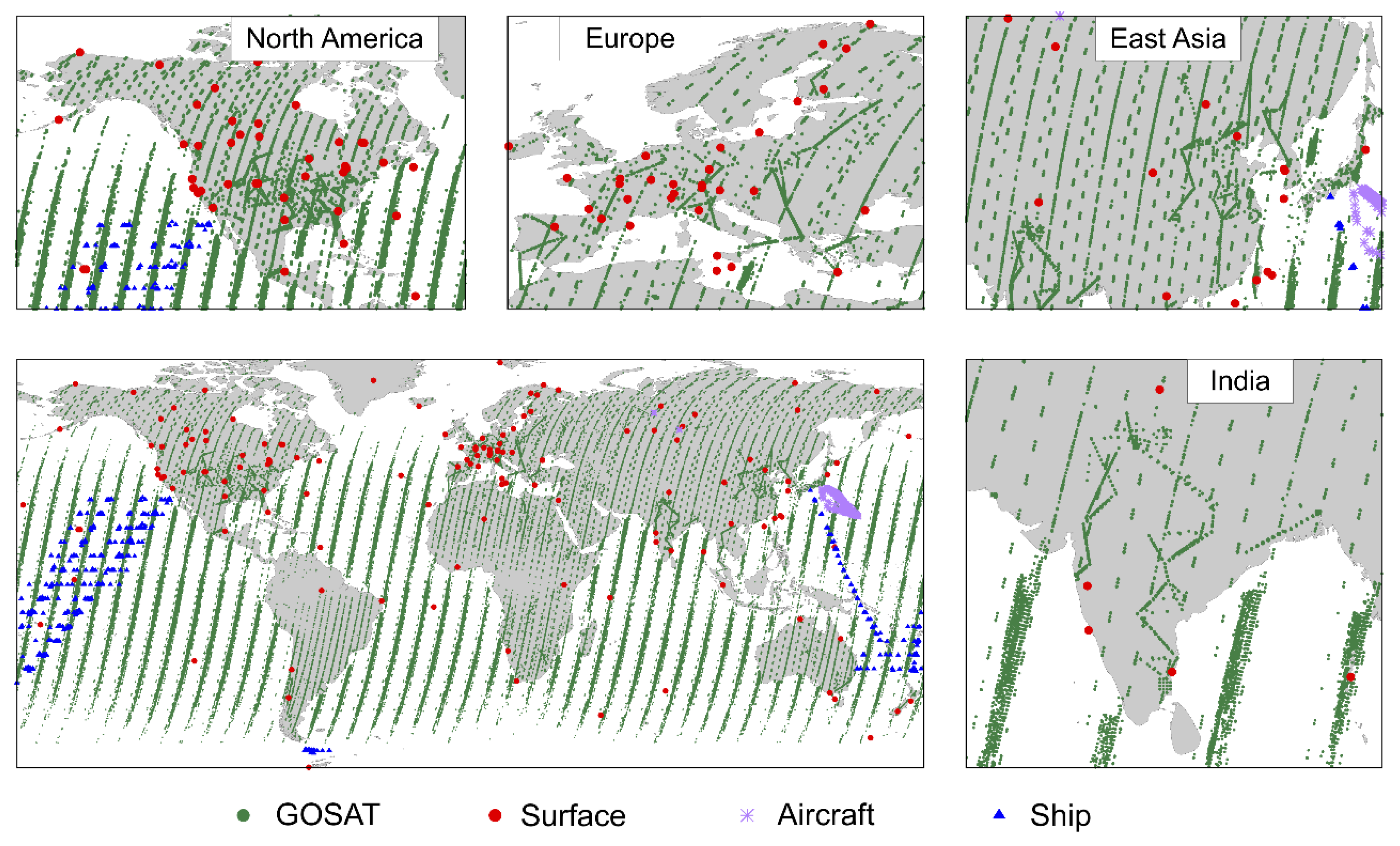
2.1. Data

In this analysis, we used methane observations from the surface observation network and satellite. The details are described in the following sections.

2.1.1. Greenhouse Gas Observing Satellite (GOSAT) Observations

The Greenhouse gases Observing Satellite (GOSAT) is a sun-synchronous satellite that observes column-averaged dry-air mole fractions of methane in the shortwave infrared band (SWIR) ([25,26]). Observations are made around 13:00 local time with a surface footprint diameter of about 10 km. In the default observation mode, it has a repeat cycle of every three days, and in the target mode, special observations are made over regions of interest. GOSAT is providing observations since June 2009 with no significant degradation of data quality ([27]). In this study, we used XCH₄ retrieved from the GOSAT at the National Institute for Environmental Studies, Japan (NIES Level 2 product, v.02.72; [28]) for the period 2011–2017 to constrain methane emissions. Data uncertainty for the GOSAT retrievals were set to 60 ppb, with the rejection threshold of 30 ppb. Such a large data uncertainty was applied to the GOSAT retrievals due to the volume of GOSAT observations being much larger than that of ground-based observations. Using a smaller uncertainty could result in an over-fit to the GOSAT data, although measurement precision is higher for the ground-based observations. The averaging kernel of GOSAT retrievals was not applied in this study because it did not affect the results in sensitivity tests.

2.1.2. Surface, Aircraft, and Ship Observations

Along with the GOSAT XCH₄ observations, ground-based weekly or continuous atmospheric CH₄ observations from a global network of stationary stations (Figure 1), aircraft and ship tracks were used in the inversions. In order to increase the representativeness of the measurements by using observations during well-mixed atmospheric conditions, the continuous observations were averaged to daily values using 12:00–16:00 local time. For mountain sites, 00:00–04:00 local time was instead used for the effects of upslope transport of local emissions due to daytime heating. For the observations from surface sites, data uncertainties were defined based on the root mean squared error (RMSE) with its prior forward simulations. A minimum threshold value of 6 ppb was set in order to allow more freedom for the inversion in the Southern Hemisphere. The rejection criteria for the surface, aircraft, and ship observations were decided based on the variance in the data (double its magnitude). Details of the data used are given in Table A1.

2.1.3. Aircraft Observations over India for Validation

Airborne CH₄ measurements were performed during Cloud Aerosol Interaction and Precipitation Enhancement Experiment (CAIPEEX) airplane campaigns around two urban areas in India ([29,30]). The measurements were done by deploying in an airplane an online in-situ cavity ring-down spectroscopy (CRDS) technique-based analyzer (G2401-m; Picarro Inc., USA). For calibration of the measurements against the World Meteorological Organization (WMO) (X2004A) scale, we measured prior to take-off three working secondary standard gasses (provided by National Oceanic and Atmospheric Administration (NOAA), Boulder, CO, USA) for 20 min each. The analyzer was monitored for pressure stability during vertical sounding. Details of the analyzer are similar to the ones reported in Chen et al. (2010) [31]. More details of observation methods could be found in Tiwari et al. 2019 [32].

2.1.4. Prior Fluxes

Prior methane fluxes used in the model included anthropogenic emissions, natural emissions from wetlands, soil sink, emissions from biomass burning, and other natural sources from the ocean, geological reservoirs, and termites. Annual anthropogenic emission was from the Emissions Database for Global Atmospheric Research (EDGAR v4.3.2) at a spatial resolution of 0.1°×0.1° ([33]) scaled to match the country reports to the UNFCCC. The scaling was applied on each grid cell based on the fractional difference in country total emissions between EDGAR and UNFCCC. The top fifteen emitting countries based on EDGAR v4.3.2 estimate for 2012 and other four countries Germany, France, United Kingdom, and Japan were selected to adjust the inventory according to UNFCCC reports (see Table A2). These nineteen countries emit 66% of the global total methane for the year 2012 ([24]). The new gridded prior emission based on the UNFCCC reports was produced by scaling the annual total to EDGAR v4.3.2 values. Beyond 2012, we used the EDGAR values for 2012. More details on the data preparation could be found in [24]. Monthly variability was incorporated using the emission seasonality data available for one year for 2010 from EDGAR. Emissions from rice cultivation were taken from EDGAR.

Emission from wetland and soil sink were estimated by Vegetation Integrative Simulator of Trace gases (VISIT, [34]) terrestrial ecosystem model simulation at 0.5°, which uses Global Lakes and Wetlands Database (GLWD; [35]) wetland area with corrections to the inundated area based on analyzed rainfall and temperature. These data were remapped from 0.5° to the model grid of 0.1° using GLWD globally, and for India using PROBA-V 100 m wetland area map from Copernicus Global Land Service ([36]), since we found several wetlands with small areal extent were missing in GLWD wetland fraction when comparing to the Indian Space Research Organization wetland atlas ([37]). Soil sink data were remapped to 0.1° resolution using the gross primary productivity (GPP) maps by MODIS MOD17 GPP product ([38]).

Emission from biomass burning was taken from Copernicus Atmosphere Monitoring Service (CAMS) Global Fire Assimilation System (GFASv1.2, [39]) daily data at 0.1° resolution. GFAS assimilates fire radiative power (FRP) observations from satellite-based sensors to produce daily estimates of biomass burning emissions. It has been extended to include information about injection heights derived from fire observations and meteorological information from the operational weather forecasts of the European Centre for Medium-Range Weather Forecasts (ECMWF). FRP observations currently assimilated in GFAS are the National Aeronautics and Space Administration (NASA) Terra and Aqua Moderate Resolution Imaging Spectroradiometer (MODIS) active fire products (http://modis-fire.umd.edu/). Data are available globally on a regular latitude-longitude grid with a horizontal resolution of 0.1 degrees.

Other emissions included annual oceanic, geological, and termite emissions. The emission from termites was from Fung et al. (1991) [40]. The emissions due to oceanic exchange were distributed over the coastal region ([41]), and mud volcano emissions were based upon Etiope and Milkov (2004) [42].

The meteorological data used for the transport model, which is described in Section 2.2.1, were obtained from the Japanese Meteorological Agency (JMA) Climate Data Assimilation System (JCDAS; [43,44]), which provides the required parameters, such as three-dimensional wind fields, temperature and humidity at 1.25°×1.25° spatial resolution, 40 vertical hybrid sigma-pressure levels, and a temporal resolution of 6 h.

2.2. Methods

2.2.1. NIES-TM-FLEXPART-VAR (NTFVAR) Inverse Modeling System

This study utilized a global Eulerian–Lagrangian coupled model NTFVAR that consists of the National Institute for Environmental Studies (NIES) model as a Eulerian three-dimensional transport model, and FLEXPART (FLEXible PARTicle dispersion model) [45] as the Lagrangian particle dispersion model (LPDM). The forward transport model and model development were reported by Ganshin et al. (2012) [46] and Belikov et al. (2016) [47]. Our transport model was a modified version of the one described in [47]. The coupled model combines NIES-TM v08.1i with a horizontal resolution of 2.5° and 32 hybrid-isentropic vertical levels described by Belikov et al. (2013) [48], and FLEXPART model v.8.0 ([45]) run in backward mode with surface flux resolution of 0.1° (resolution of available surface fluxes limits resolution of the Lagrangian model). The changes in the current version with respect to the study by [47] include revision in the transport matrix, indexing and sorting algorithms to allow efficient memory usage for handling large matrixes of Lagrangian responses to surface fluxes required when using GOSAT data in the inversion. More details could be found in [24].

2.2.2. The Inverse Modeling Scheme

We used a high-resolution version of the transport model and its adjoint described by Belikov et al. (2016) [47], which was combined with the optimization scheme proposed by Meirink et al. (2008) [49] and Basu et al. (2013) [50]. Following the approach by [49], flux corrections were estimated independently for two categories of emissions viz. anthropogenic and natural. Variational optimization was applied to obtain flux corrections as two sets of scaling factors to monthly varying prior uncertainty fields at 0.1°×0.1° resolution separately for anthropogenic and natural wetland emissions with a bi-weekly time step. Corrections to the anthropogenic emission were according to the monthly climatology of emissions provided by EDGAR, and wetland emissions were proportional to the monthly climatology of wetland emissions by the VISIT model, both given as prior uncertainty fields. The grid-scale flux uncertainty was defined as 30% of EDGAR climatology for the anthropogenic flux category and 50% of VISIT climatological emissions for the wetland emission category. No optimization was applied to other natural flux categories, such as emissions from biomass burning, geological sources, termites, and soil sink, as their amplitude is an order of magnitude less than that of wetlands. A spatial correlation length of 500 km and a temporal correlation of two weeks were used to provide smoothness on the scaling factors. The inverse modeling problem was formulated ([49,51]) as the solution for the optimal value of

x

– vectors of corrections to prior fluxes at the minimum of a cost function

J (x)

:

J (x) = \frac{1}{2} {(H \cdot x - r)}^{T} \cdot R^{- 1} \cdot (H \cdot x - r) + \frac{1}{2} x^{T} \cdot B^{- 1} \cdot x

(1)

where H is the atmospheric transport operator, r is the difference between observed concentration and forward simulation made with prior fluxes without correction, R is the covariance matrix of observations, and B is the covariance matrix of fluxes. In the B matrix design, we followed [49] in representing B matrix as multiple of non-dimensional covariance matrix C and the diagonal flux uncertainty D as

B = D^{T} \cdot C \cdot D

(2)

C matrix is commonly implemented as a band matrix with non-diagonal elements declining as

~ \exp (- l^{2} / d^{2})

with distance l between the grid cells and d the correlation distance. The optimal solution, as the minimum of the cost function J, was calculated iteratively with an efficient Broyden–Fletcher–Goldfarb–Shanno (BFGS) algorithm, as implemented by [52]. More details on the implementation could be found in [24,53].

2.2.3. Posterior Uncertainties

Posterior flux uncertainties were calculated from a set of five simulations by randomly perturbing the observations and the prior fluxes, as in the method described by [54]. Pseudo-observations were prepared by perturbing the observations with its uncertainty at each site. Also, prior monthly EDGAR and VISIT fluxes were prepared, applying random scaling factors separately for each global carbon project (GCP) region and month. Inversions were carried out using the perturbed pseudo-observations and the perturbed fluxes (perturbed EDGAR and VISIT combined with non-perturbed soil sink, biomass burning, and other natural emissions from the ocean, geological sources, and termites) as the prior fluxes and calculating the standard deviation of the inversion results.

3. Results

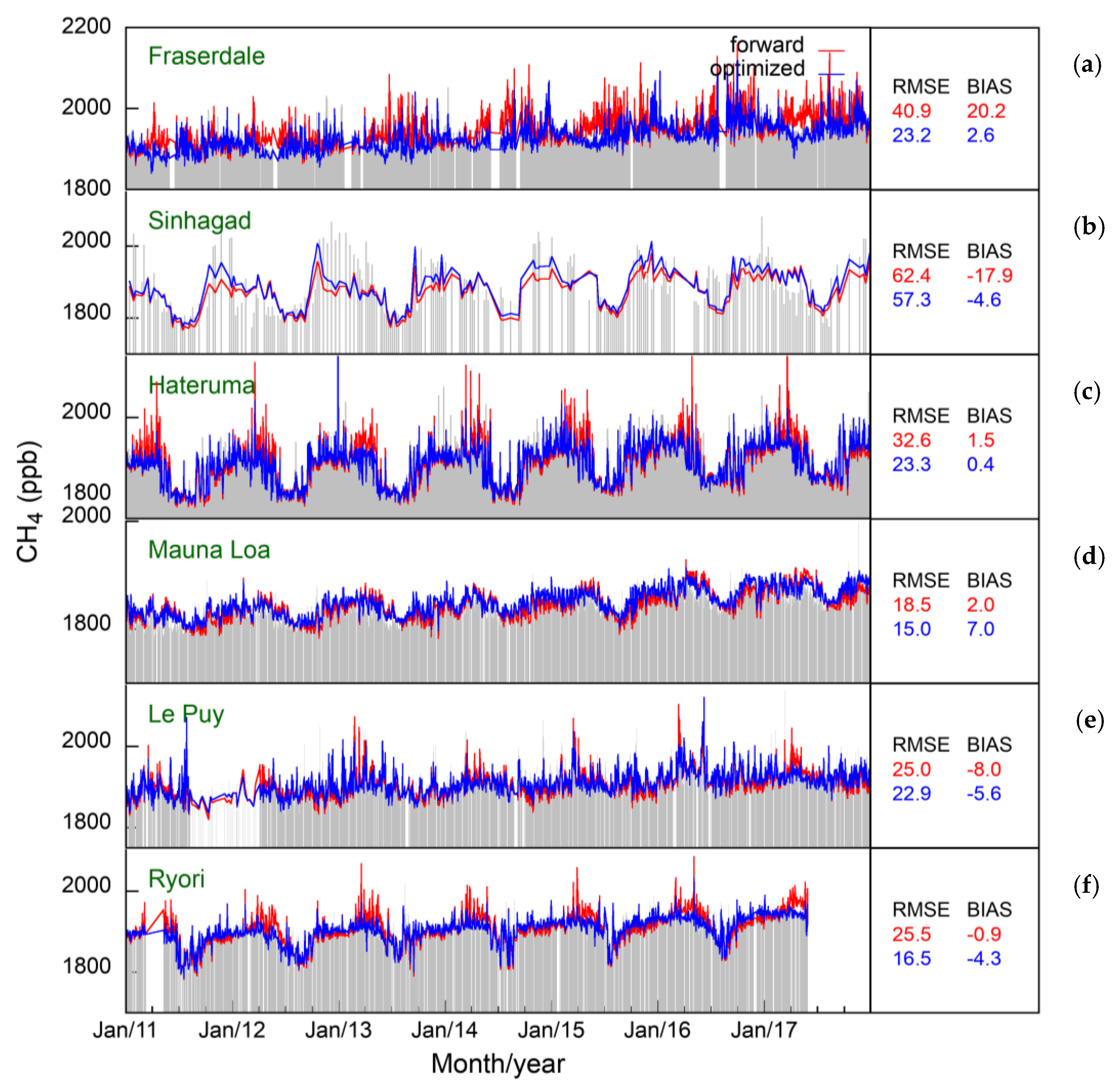
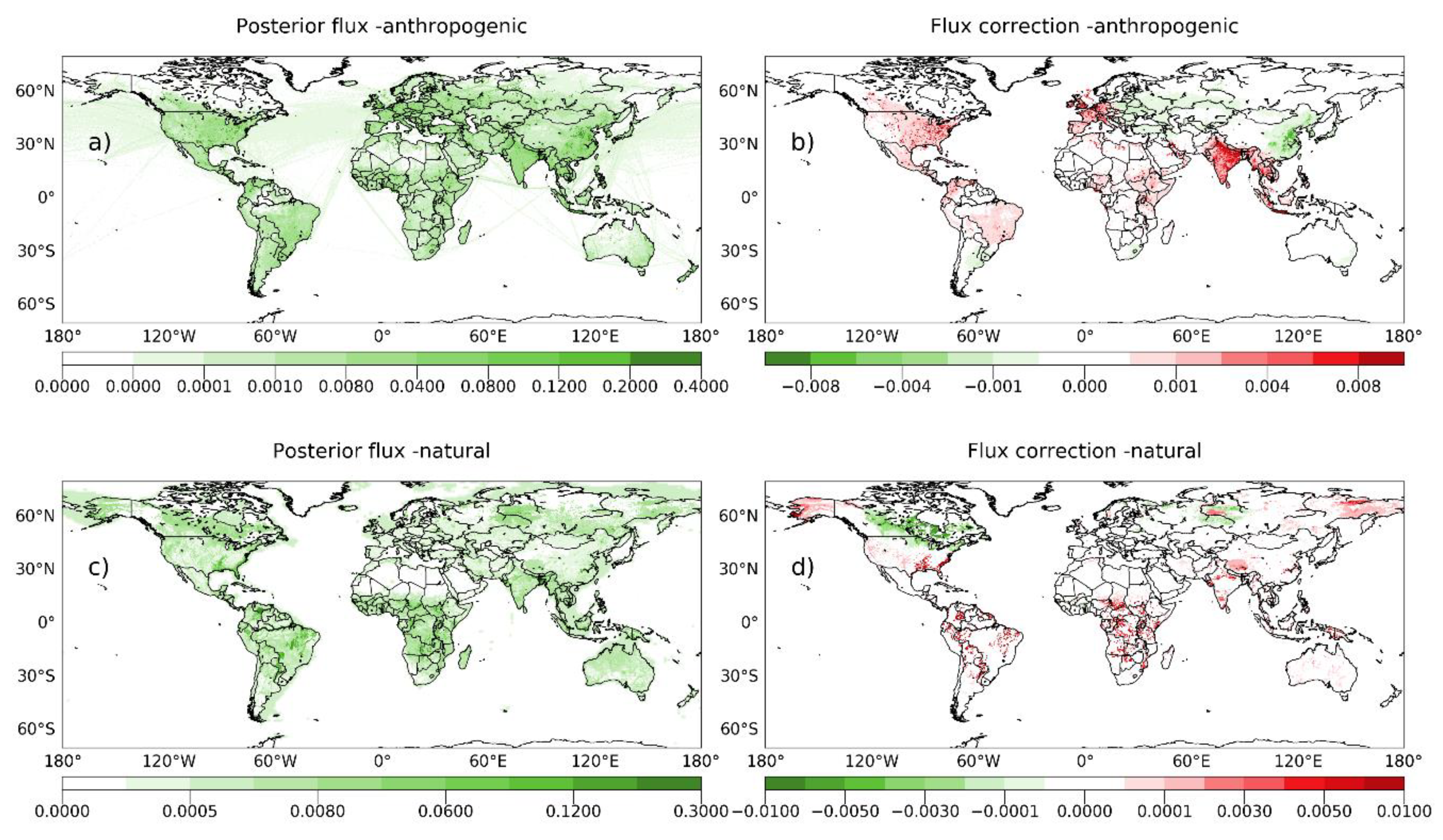
3.1. Posterior Fluxes and Flux Corrections

In this study, two categories of fluxes, viz. natural and anthropogenic, were optimized by the inverse model. The annual mean (for the entire study period) global total natural prior was 209.15 Tg CH₄ yr⁻¹, and the posterior estimated was 232.49 Tg CH₄ yr⁻¹. This was in close agreement with top-down estimates reported in Saunois et al. (2016) [55] (234 Tg), but higher than Saunois et al. (2019) [2] (215 Tg). In the case of anthropogenic emissions, the prior was 342.57 Tg CH₄ yr⁻¹, and the posterior was 340.92 Tg CH₄ yr⁻¹_, which was between 319 and 357 Tg estimated by [55] and [2], respectively. The global total methane emission prior and posterior were 551.73 and 573.40 Tg CH₄ yr⁻¹, respectively; the total posterior emission was close to the estimate of 572 Tg by [2]. Figure 2 presents the comparison of surface methane observations, prior forward simulation and optimized forward for six surface measurement sites, including Fraserdale (Canada), Sinhagad (India), Hateruma (Japan), Mauna Loa (United States), Le Puy (France), and Ryori (Japan). Fraserdale is a continental site with large CH₄ variability due to local wetland emissions. Sinhagad is a mountain site, whose CH₄ concentration is influenced by maritime air in summer and inland emissions during winter due to seasonal reversal of wind patterns. Mauna Loa is considered as a global background station, and Hateruma and Ryori are influenced by emissions from East Asia. The inversion optimized fluxes brought down the RMSE and bias compared to the prior forward simulations.

On a regional scale, anthropogenic emissions were found to increase in posterior compared to the prior over North America, tropical South America, Western Europe, tropical Africa, and Southeast Asia. Reductions were observed mainly over eastern Europe, China, Middle East countries, Japan, temperate South America, and southern parts of Southern Africa. These were in conformity with some studies, for example, the overestimation of Chinese coal emissions and the oil and gas sector in the Middle East in EDGAR ([56]), although we did not attribute these differences to any source sectors. The posterior fluxes in the natural emission category increased over tropical South America, contiguous and central North America, Southern Africa, parts of India, China, and Southeast Asia, and eastern parts of Russia. Amazonia is the largest natural tropical source of methane, still have large uncertainty in the emission ([57]), and some studies have reported upward revision in the inverse analysis (e.g., [58]). Tropical Africa is also a natural methane emitter (12% of global wetland emission, [59]) where the sources are wetlands, flood plain, riverine ecosystems, etc. Due to the seasonal migration of the intertropical convergence zone (ITCZ), the inundation extent is highly variable in these water bodies, and thus there is significant variability in the estimates of methane emission in this region ([60]) and difficulty in models to capture the wetland emissions. Significant reductions were observed over boreal North America and Russia (Figure 3). It should be noted that the administrative boundaries shown in Figure 3 and Figure 4 are approximate and might deviate from areas for which national emissions are reported or the national boundaries defined by the countries. Detailed analysis on the country scale is described in the following section.

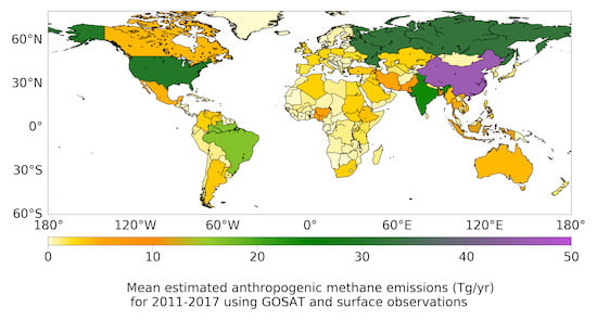
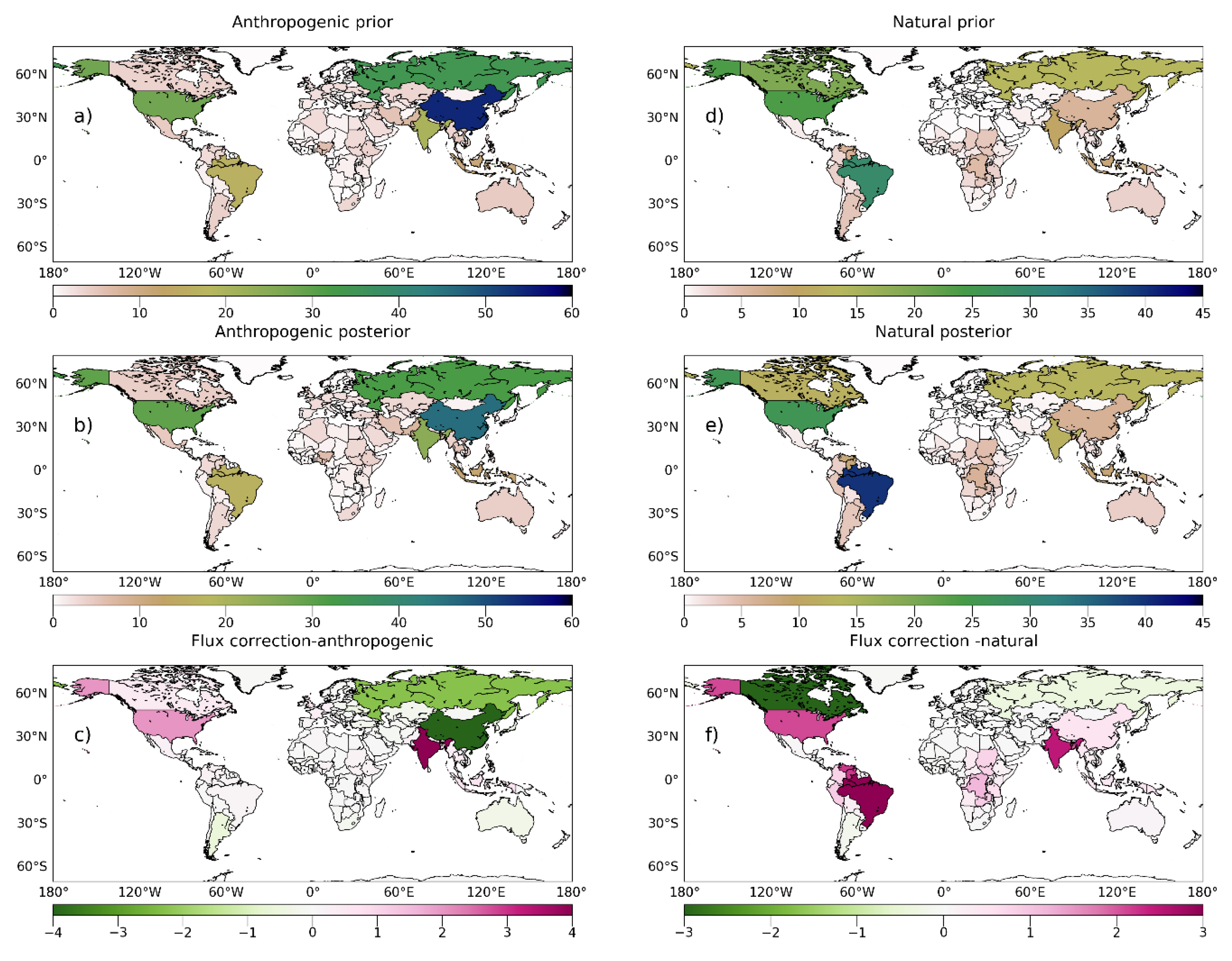
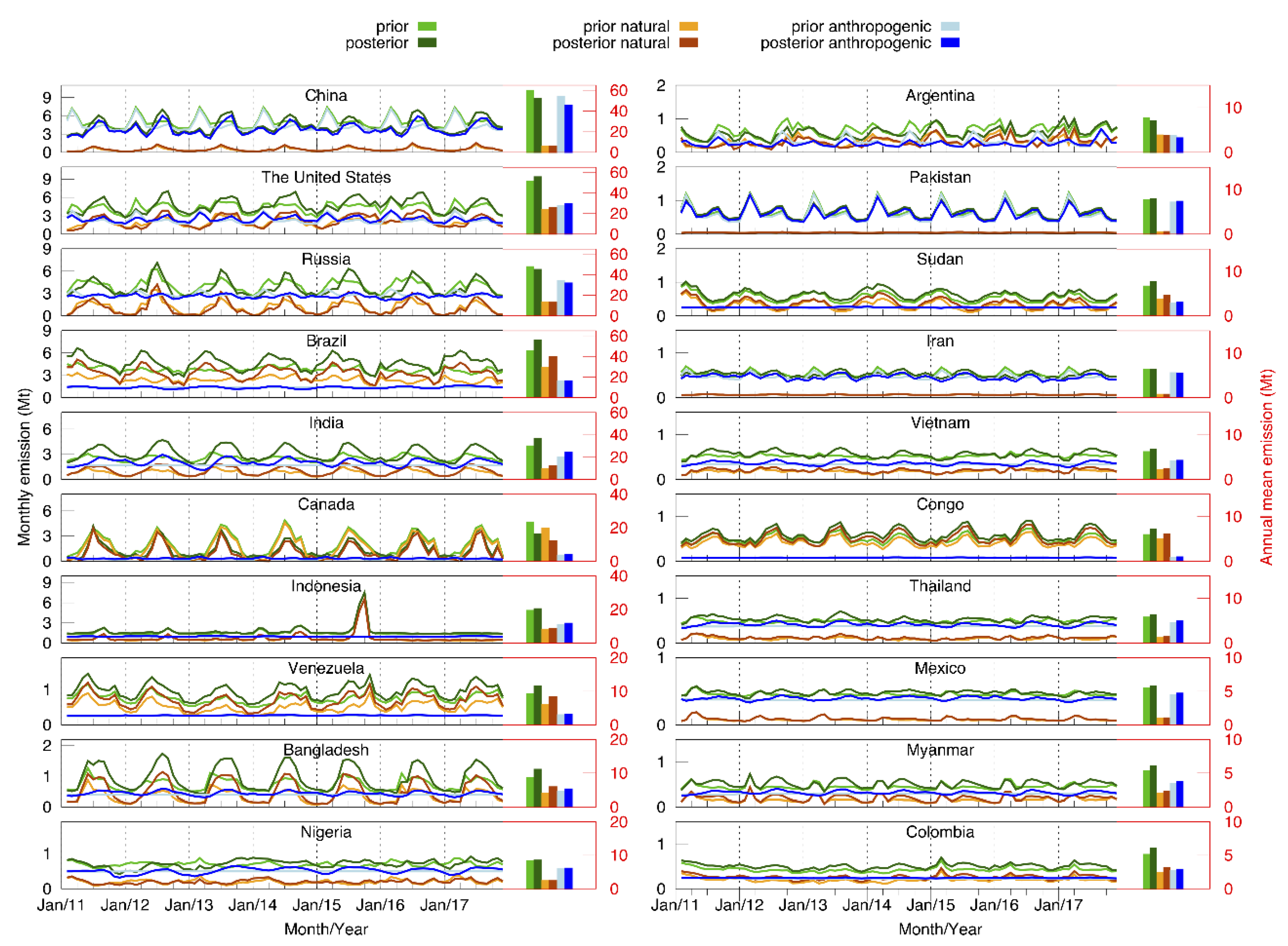
3.2. Country Total Emissions

3.2.1. Emission from Anthropogenic Sources

We analyzed the prior and posterior emissions for anthropogenic and natural categories and their flux corrections by the inverse model on a country scale (Figure 4). For the anthropogenic category, emission totals calculated from EDGAR prior were highest for China (54.3 Tg CH₄ yr⁻¹), Russia (34.2 Tg CH₄ yr⁻¹), United States (27.8 Tg CH₄ yr⁻¹), India (20.1 Tg CH₄ yr⁻¹), and Brazil (16.4 Tg CH₄ yr⁻¹). The inverse model corrected the prior emission upward for India 24.18 ± 5.3 Tg CH₄ yr⁻¹ (difference: 4.1 Tg; 20.4%) and United States 29.76 ± 7.8 Tg CH₄ yr⁻¹ (2 Tg; 7.2%), while reduction in posterior emissions found over China 45.73 ± 8.6 Tg CH₄ yr⁻¹ (8.6 Tg; 15.8%), Russia 31.91 ± 7.8 Tg CH₄ yr⁻¹ (2.25 Tg; 6.6%). Among countries having large anthropogenic emissions, emission from Brazil was having the least correction (0.1 Tg CH₄ yr⁻¹; 0.61%). Anthropogenic prior total emission in Indonesia was 11.17 Tg CH₄ yr⁻¹, which was found to have a 5.8% upward correction of 0.65 Tg so that the posterior emission was 11.82 ± 2.5 Tg. The prior, posterior, and percentage difference in posterior for natural, anthropogenic, and total emissions for selected countries is shown in Table 1. Considering the posterior uncertainty for each country, most of the large emitting countries were found to have the inverse model corrections within the model uncertainty range, which was calculated, as mentioned in Section 2.2.3. Though in the case of India, the optimized emission was higher than the anthropogenic prior, the difference was within the inverse model uncertainty (4.1 Tg against 5.3 Tg uncertainty).

3.2.2. Emission from Natural Sources

In our study, though we optimized only for wetland emissions, the discussions were on total natural emissions, including other natural sources. In the case of emissions from natural sources, the largest upward corrections were for northern South American countries, such as Venezuela (2.22 Tg CH₄ yr⁻¹; 36.27%), Colombia (0.78 Tg CH₄ yr⁻¹; 32.77%), and Brazil (10.5 Tg CH₄ yr⁻¹; 36%) and a lower posterior emissions in Argentina (0.14 Tg CH₄ yr⁻¹; 3.5%) in South America. Other South American countries, such as Peru and Bolivia, also had a more than 20% increase in the posterior emissions compared to prior. Thus, there is a general tendency that the northern South American countries have lower emissions from natural sources in the prior. While the United States had 2.1 Tg CH₄ yr⁻¹ increase, which was 8.8% of the natural prior, posterior emissions in Canada was 7.4 Tg CH₄ yr⁻¹ (37.8%) less than prior, which was still within the uncertainty range of the prior emissions. In Asia, for India and Bangladesh, there are large positive corrections to emissions (2.48 Tg CH₄ yr⁻¹; 25% and 1.89 Tg CH₄ yr⁻¹; 46.9%, respectively), followed by a less but positive correction in China mainland (0.45 Tg CH₄ yr⁻¹; 7.7%). The inverse model suggested an overall underestimation in the prior for equatorial African countries (Figure 4f), such as Uganda, Tanzania, Sudan, and Kenya, though the annual emissions were lower for these countries. A recent study ([60]) using GOSAT XCH₄ observations in their inversion reported overall larger emissions compared to prior over Africa with strong exceptions in the Congo basin. However, in our analysis, we found a slight increase in our posterior emissions over the Democratic Republic of Congo. They attributed the increase in the CH₄ emissions during 2010–2015 to increase the wetland extent during this period in some regions of Sudan (Sudd wetland). Tootchi et al. (2019) [61] presented the details of the disparity in the spatial extent among different wetland datasets over this region (Figure 10 therein). In their study, the Baroste floodplain in southern tropical Africa had a wetland extent ten times that during the dry season minimum. Thus, there was potentially an underestimation in our prior wetland model over this area. More details of emission from these countries could be found in Table 1.

4. Discussion

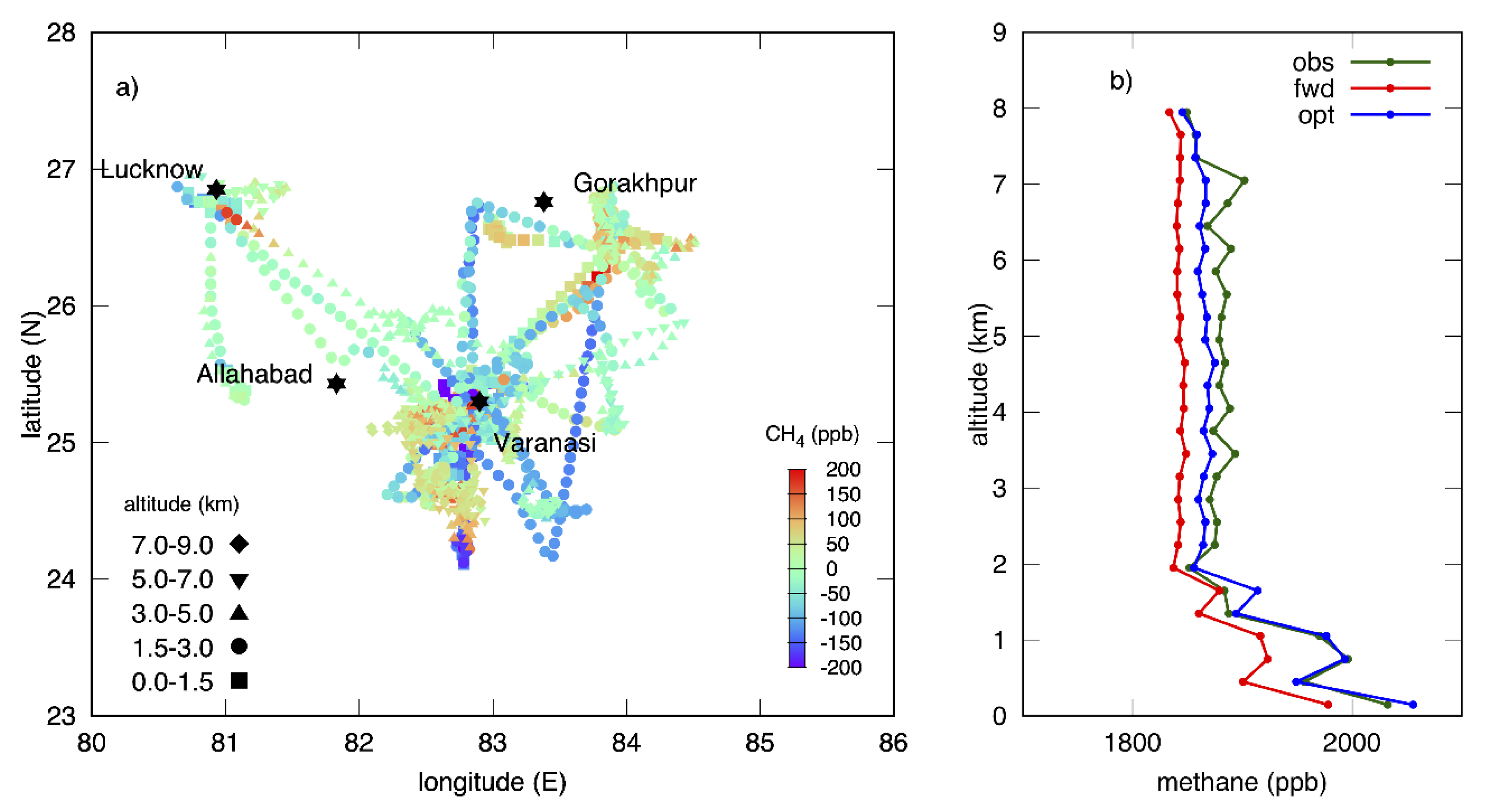
4.1. Case of India

As far as the methane emission from India is concerned, there are large differences in the total wetland area in different wetland area databases. For example, Adam et al. (2010) [62] addressed the issue of disparity between GLWD wetland areas and satellite-based estimation of naturally inundated areas (NIA). Their study showed that the difference between GLWD and NIA in India and Southeast Asia (among other regions in their study) covered a significant area. Though satellite-based inundation extent might be overestimated in areas where wet soils could be interpreted as inundated, in the Indian subcontinent, they showed that GLWD might be missing some waterbodies. Therefore, there is a possibility that the wetland methane emissions in India may be underestimated in the prior (as suggested by increasing the wetland emissions by optimization), and this may influence the posterior estimate of anthropogenic emissions due to the lack of freedom to increase wetland emissions because of underestimated wetland area fraction in the region. In our analysis, we found that in India, some wetlands with small areal extent were not captured in GLWD dataset, and we merged it with the PROBA-V 100 m wetland area fraction to redistribute spatially the 0.5° wetland methane emissions from VISIT model, keeping the total India wetland emissions unchanged.

Moreover, the anthropogenic emissions for India in EDGAR v4.3.2 is around 65% higher than the UNFCCC reported data (for example, in 2010, the EDGAR estimate is 32.6 Tg, while the emission reported to UNFCCC is 19.7 Tg in first Biennial Update Report to the UNFCCC by the Government of India ([63]) and 21 Tg in 2008 by [64]). Some of the recent studies, focusing on the region, covering some of the years in this analysis, found emission estimates between UNFCCC reports and the recent EDGAR updates. For example, Miller et al., (2019) [7] estimated lower anthropogenic emission for India than EDGAR 4.3.2 but higher annual emissions than Ganesan et al., (2017) [65]. Both the studies used GOSAT observations, and [65] also included surface and aircraft observations of methane in India in their inversion. Here, in our analysis, to constrain the emissions in the region, observations from four surface stations (Sinhagad; SNG [66], Cape Rama; CRI [67], Port Blair; PBL, and Pondicherry; PON [68]) in the Indian subcontinent were included in the inversion. The RMSE and bias for all four stations were reduced after the optimization by the inverse model. The RMSE for SNG was reduced to 57.4 in optimized simulation from 62.5 of prior forward and the bias from −17.9 to −4.6. Similarly, for CRI station (RMSE from 50.9 to 37.9 and bias from −23.4 to −9.4), PBL (RMSE from 40.9 to 34.8 and bias from −14.6 to −5.5), and PON (RMSE from 50.4 to 39.4 and bias from −32 to −16.7).

As a validation to the inverse model estimates, we prepared an independent check with aircraft observations of methane during few months for 2014 (September to November) and 2015 (July). This aircraft observation campaign was conducted by the Indian Institute of Tropical Meteorology, India (Section 2.1.3). These observations were not included in our inversion itself, but prior forward and optimized forward simulations were carried out for one-minute averaged CH₄ observations. Figure 5a shows the tracks of aircraft observations centered around the Indian city of Varanasi and the difference between the observations and simulation with fluxes optimized by the inverse model. Flight tracks of the observations around the city of Pune, which were also used in the profile averaging presented in Figure 5b, were not shown here. The vertical profiles of the aircraft CH₄ observations averaged for 300 m altitude is shown in Figure 5b. The total methane emission, both anthropogenic and natural, in India, was corrected upwards by the optimization. It could be seen in Figure 5b that the prior forward simulation showed low mixing ratios at all mean vertical levels, and the simulations with posterior emissions agreed well in the boundary layer and to a less degree above it. Overall, the validation with the surface stations was used in the inversion and the aircraft observations used for validation only, and the posterior simulations showed a better fit to the observations than the prior forward model.

4.2. Seasonal Variability in Emission

Besides the annual country’s total emissions, we analyzed the monthly variation of the fluxes for selected countries (having total emission greater than 5 Tg yr⁻¹), as presented in Figure 6. In the case of China, the peak anthropogenic emission during the spring season was reduced, and the posterior emissions peaked during the summer months. The relatively lower natural methane emissions had not been altered by the inverse model. Anthropogenic prior for India showed a very weak seasonal cycle (similar to the analysis by [65]), while the inverse model brought out the more significant seasonal cycle with peaks during the southwest monsoon season (June to September). This was due to the fact that agricultural practices are dependent on rainy season (e.g., ~40% of rice production in low-lying rainfed land, [69]), and a slight phase shift with natural sources was found with the emission from natural sources (Figure 6), which indicates sources other than in natural emission category. Waterlogged areas increased nearly threefold during the southwest monsoon season, resulting in increased wetland CH₄ emissions ([70]). During this season, the natural emission also increased in the posterior (e.g., [71]), both contributing to the summer peak in the total methane emission in India. Bangladesh had a very clear seasonal cycle (further enhanced by the optimization), which was mainly modulated by the methane emission from the natural sources. Pakistan had a peculiar scenario, having very small emission from natural sources with the total methane emission having distinct double peaks, a dominant one in spring and another one in summer. Most of the methane emission in Pakistan was from the agricultural sector (4 Tg in 2012, [72]). Iran also showed large influence from anthropogenic sources, and the inverse model offset the emission peak to summer months from spring. The natural methane emission in Russia was almost half of the total anthropogenic emissions, but the amplitude of the monthly variation was large compared to anthropogenic emissions, and thus the seasonality in total methane emission was modulated by natural emissions.

In the Southeast Asian countries, emission from natural sources is mainly influenced by water availability due to summer monsoon (e.g., [73]). Although the anthropogenic emission is larger than the emission from natural sources in Indonesia, there are strong signals of natural emissions due to major fire events in Indonesia (e.g., anomalous peak in 2015). Total methane emission in Myanmar has two peaks in monthly emissions, one in spring and another prominent peak in summer monsoon season. Myanmar is a country influenced by southwest monsoon rainfall and is a land of rice production both irrigated and rainfed ([74]), of which the majority of CH₄ emission (65%) is from irrigated or deep-water rice fields. Thus, the seasonality in CH₄ emissions is mainly modulated by wetland emissions. Variability in total emission follows mainly the variability in natural emissions. Methane emission in Thailand is, on the other hand, influenced mainly by anthropogenic emissions. So is the case with Vietnam, the optimization embeds a stronger annual peak during the monsoon season.

For the United States, these two categories are nearly equal in magnitude, but peaks at different seasons in the year-−natural emissions in summer and anthropogenic in winter. The main anthropogenic source of methane in the United States is from livestock and manure management. The seasonality in methane emission in Canada is driven mainly by natural emissions, which has a larger magnitude than the anthropogenic emissions [75]. The seasonal cycle in the total methane emission in Mexico is mainly contributed by the anthropogenic emissions, with more than four times the emission from natural sources. In Brazil, the seasonality in the total methane emission is mainly driven by variability in methane emissions from natural sources, and in the posterior, we found substantial upward correction in the natural emission category and thereby total methane emissions. Besides Brazil, Venezuela also is mainly contributed by emission from natural sources with a distinct peak during summer months. While seasonality in the methane emission in Colombia is influenced mainly by natural sources, the seasonal cycle in total emission in Argentina is equally modulated by natural and anthropogenic categories.

In the African continent, Nigeria, Sudan, and the Democratic Republic of Congo are the main methane emitters. Though anthropogenic emission is the major category of emission and has clear seasonality in Nigeria, the total emissions do not have a discernible seasonal pattern in emission. On the contrary, Sudan and Congo have a clear seasonal cycle due to the greater contribution from natural sources.

4.3. Desirable Future Improvements

The deficiencies of the inversion system, with respect to the application for comparison of estimated emissions with national emission reports, to be addressed in future studies include the following. The inverse model optimizes the emissions on a coarser spatial resolution than the transport defined on 0.1° because of smoothing in the flux corrections applied to the prior emissions, which is dependent on both the smoothness constraint and the number of iterations. Thus, more research is needed to find an optimal balance between the smoothness of the solution and the amount of detail in retrieved fluxes. It would potentially improve the estimated emissions for countries and regions with lower emissions. Another improvement should be the use of high-resolution meteorological fields for transport, in place of currently used data at 1.25° spatial resolution and 6 h temporal intervals ([76,77]). Improved mapping of natural (and anthropogenic) emissions is necessary as we have identified deficiencies in the spatial distribution of wetland emissions, for example, over India, as discussed in Section 4.1. Some of the transport model biases, such as reduced vertical mixing and higher inter-hemispheric transport rate in the Eulerian transport model, used in this study were discussed in a multi-model intercomparison study by Krol et al. (2018) [78]. Currently, there is less evidence on the size of the biases and their impact on inversion results; more details would emerge after analysis of the data of GCP methane intercomparison ([2]), where multiple models could be compared to each other, including the one used in this study, and the correlations between transport model properties and reconstructed emissions could be established. Unaccounted biases in the satellite observations, especially over regions where ground-based observations are missing, also might influence the results. Incorporating more ground-based observations in the inversion might help reducing biases over regions with a sparse observation network.

5. Conclusions

We carried out inversion of methane fluxes for seven years using GOSAT satellite observations and surface observations using a high-resolution inverse model NIES-TM-FLEXPART-VAR (NTFVAR) that couples a Lagrangian particle dispersion model FLEXPART with a global Eulerian model NIES-TM. Optimization was applied to natural (wetland only) and anthropogenic emissions on a bi-weekly time step, and the results were analyzed on a global country scale. In order to evaluate the inverse model estimates of methane emissions on a country scale, we used EDGAR anthropogenic methane emission inventory scaled to match the national reports to the UNFCCC. Our results showed that largest correction to the wetland emissions were for Bangladesh having an upward revision of around 46.9% (1.89 Tg CH₄ yr⁻¹) of its prior, followed by Venezuela (2.2 Tg CH₄ yr⁻¹; 36.3%), Brazil (10.5 Tg CH₄ yr⁻¹; 36.1%), and India (2.4 Tg CH₄ yr⁻¹; 25.2%), while there was 37.8% (7.5 Tg CH₄ yr⁻¹) reduction for Canada. On the other hand, anthropogenic emission was found to differ from national reports for the United States by 2 Tg CH₄ yr⁻¹ (7.2%), China (8.6 Tg CH₄ yr⁻¹; 15.8%), India (4.1 Tg CH₄ yr⁻¹; 20.4%), Russia (2.3 Tg CH₄ yr⁻¹; 6.6%), Canada (0.5 Tg CH₄ yr⁻¹; 12.4%), Bangladesh (0.6 Tg CH₄ yr⁻¹; 13.7%, and Argentina (0.6 Tg CH₄ yr⁻¹; 14.7%), with all differences being within emission uncertainty range. The inversion results for India were validated against aircraft data over two north Indian urban regions, and the posterior fit to the observations showed a clear improvement, especially in the boundary layer. The application of an inversion system based on high-resolution transport using prior anthropogenic emission field adjusted to the UNFCCC emission reports, and with the combination of surface and satellite observations, enabled us to study the natural and anthropogenic methane emissions over a spatial scale of countries and to compare with the national methane emission reports. However, improvements in the resolution of the model and meteorological fields, fixing source allocations in emission sources used as priors, refinements to reduce model and observation biases, and inclusion of more observations are desirable targets for future improvement.

Author Contributions

Study design, R.J. and S.M.; methodology, S.M., R.J., A.T. and F.W.; software, S.M.,A.T. and R.J.; simulations, R.J., A.T., and F.W.; validation, R.J. and S.M.; formal analysis, R.J.; investigation, R.J. and S.M.; resources, T.M.; data curation, Y.K.T., A.I., J.W.K., G.J.-M., M.A., M.S., Y.T., E.J.D., D.E.J.W., M.R., J.A., J.V.L., S.P., P.B.K., R.L.L., Y.Y., I.M., and T.M.; writing—original draft preparation, R.J.; writing—review and editing, R.J., S.M., F.W., A.T., V.V., Y.K.T., I.M., J.V.L., and D.E.J.W.; visualization, R.J.; supervision, S.M.; project administration, T.M.; funding acquisition, T.M. All authors have read and agreed to the published version of the manuscript.

Funding

This research was supported by the GOSAT project at the National Institute for Environmental Studies, Japan.

Acknowledgments

We thank all the people and institutes who procured and provided the observation data used in this study. We are grateful to Emilio Cuevas, Juha Hatakka, Petri Keronen, Elena Kozlova, Tuomas Laurila, Zoe Loh, Nikolaos Mihalopoulos, Simon O’Doherty, Ray Wang, Damiano Sferlazzo, and other contributors making the methane observations and data available for the Global Carbon Project. We thank the Ministry of the Environment, Japan, for the financial support for the GOSAT project. The simulations were carried out using the Supercomputer System of the National Institute for Environmental Studies (NIES). We thank Dr. Thara Prabhakaran, CAIPEEX Project Head, and team of scientists involved in this project for supporting GHGs monitoring during the airplane campaign. The CAIPEEX project is funded by the Ministry of Earth Sciences, Government of India.

Conflicts of Interest

The authors declare no conflict of interest.

Appendix A

Table A1. List of observations used in this inversion. The details are Station (country), site ID, institute conducting observations, observation type, and sampling method.

Station	Observation ID	Lab	Observation Type	Sampling Type
Abbotsford (Canada)	abb006	ECCC	Station	Continuous
Arembepe (Brazil)	abp001	NOAA	Station	Discrete
Alert (Canada)	alt006	ECCC	Station	Continuous
Alert (Canada)	alt001	NOAA	Station	Discrete
Amsterdam Island (France)	ams011	LSCE	Station	Discrete/Continuous
Argyle (US)	amt001	NOAA	Station	Discrete
Anmyeon-do (Republic of Korea)	amy061	KMA	Station	Continuous
Aircraft (Western North Pacific) (Japan)	aoa019	JMA	Aircraft	Discrete (aircraft)
Arrival Heights (New Zealand)	arh015	NIWA	Station	Discrete
Ascension Island (United Kingdom)	asc001	NOAA	Station	Discrete
Assekrem (Algeria)	ask001	NOAA	Station	Discrete
Amazon Tall Tower Observatory (Brazil)	ato045	MPI-BGC	Station	Continuous
Serreta (Portugal)	azr001	NOAA	Station	Discrete
Azovo (Russia)	azv	NIES	Station	Continuous
Baltic Sea (Poland)	bal001	NOAA	Station	Discrete
Boulder (US)	bao001	NOAA	Station	Discrete
Behchoko (Canada)	beh006	ECCC	Station	Continuous
Begur (Spain)	bgu011	LSCE	Station	Discrete
Baring Head (New Zealand)	bhd001	NOAA	Station	Discrete
Biscarrosse (France)	bis011	LSCE	Station	Continuous
Bukit Kototabang (Indonesia)	bkt105	EMPA	Station	Continuous
Bukit Kototabang (Indonesia)	bkt001	NOAA	Station	Discrete
St. David’s Head (United Kingdom)	bme001	NOAA	Station	Discrete
Tudor Hill (Bermuda) (United Kingdom)	bmw001	NOAA	Station	Discrete
Bratt’s Lake (Canada)	brl006	ECCC	Station	Continuous
Barrow (US)	brw001	NOAA	Station	Discrete
Berezorechka (Russia)	brz	NIES	Station	Continuous
Constanta (Black Sea) (Romania)	bsc001	NOAA	Station	Discrete
Pacific Ocean (New Zealand)	bsl015	NIWA	Ship	Discrete
Cambridge Bay (Canada)	cab006	ECCC	Station	Continuous
Cold Bay (US)	cba001	NOAA	Station	Discrete
Cabauw (Netherlands)	cbw196	RUG	Station	Continuous
Cape Ferguson (Australia)	cfa002	CSIRO	Station	Discrete
Cape Grim (Australia)	cgo001	NOAA	Station	Discrete
Cape Grim (Australia)	cgo043	AGAGE	Station	Continuous
Chapais (Canada)	cha006	ECCC	Station	Continuous
Chibougamau (Canada)	chi006	ECCC	Station	Continuous
Christmas Island (Kiribati)	chr001	NOAA	Station	Discrete
Cherskii (Russia)	chs001	NOAA	Station	Discrete
Churchill (Canada)	chu006	ECCC	Station	Continuous
Valladolid (Spain)	cib001	NOAA	Station	Discrete
Monte Cimone (Italy)	cmn106	UNIURB/ISAC	Station	Discrete
Cape Ochiishi (Japan)	coi020	NIES	Station	Continuous
Cape Point (South Africa)	cpt036	SAWS	Station	Continuous
Cape Point (South Africa)	cpt001	NOAA	Station	Discrete
Cape Rama (India)	cri002	CSIRO	Station	Discrete
Crozet (France)	crz001	NOAA	Station	Discrete
Casey (Australia)	cya002	CSIRO	Station	Discrete
Demyanskoe (Russia)	dem020	NIES	Station	Continuous
Downsview (Canada)	dow006	ECCC	Station	Continuous
Drake Passage (US)	drp001	NOAA	Ship	Discrete
Dongsha Island (Taiwan)	dsi001	NOAA	Station	Discrete
Egbert (Canada)	egb006	ECCC	Station	Continuous
Easter Island (Chile)	eic001	NOAA	Station	Discrete
CONTRAIL (Japan)	eom010	MRI	Aircraft	Discrete (aircraft)
Estevan Point (Canada)	esp006	ECCC	Station	Continuous
Esther (Canada)	est006	ECCC	Station	Continuous
East Trout Lake (Canada)	etl006	ECCC	Station	Continuous
Finokalia (Greece)	fik011	LSCE	Station	Discrete
Fraserdale (Canada)	fsd006	ECCC	Station	Continuous
Gif-sur-Yvette (France)	gif011	LSCE	Station	Continuous
Giordan Lighthouse (Malta)	glh209	UMIT	Station	Continuous
Guam (US)	gmi001	NOAA	Station	Discrete
Gunn Point (Australia)	gpa002	CSIRO	Station	Discrete
Gosan (Republic of Korea)	gsn	NIER	Station	Continuous
Hateruma Island (Japan)	hat020	NIES	Station	Continuous
Halley (United Kingdom)	hba001	NOAA	Station	Discrete
Hanle (India)	hle011	LSCE	Station	Discrete
Hohenpeissenberg (Germany)	hpb001	NOAA	Station	Discrete
Hegyhatsal (Hungary)	hun001	NOAA	Station	Discrete
Storhofdi (Iceland)	ice001	NOAA	Station	Discrete
Igrim (Russia)	igr020	NIES	Station	Continuous
Inuvik (Canada)	inu006	ECCC	Station	Continuous
Izaña (Spain)	izo001	NOAA	Station	Discrete
Izaña (Spain)	izo027	AEMET	Station	Continuous
Jungfraujoch (Switzerland)	jfj005	EMPA	Station	Continuous
Key Biscane (US)	key001	NOAA	Station	Discrete
Kollumerwaard (Netherlands)	kmw196	RIVM	Station	Continuous
Karasevoe (Russia)	krs020	NIES	Station	Continuous
Cape Kumukahi (US)	kum001	NOAA	Station	Discrete
Sary Taukum (Kazakhstan)	kzd001	NOAA	Station	Discrete
Plateau Assy (Kazakhstan)	kzm001	NOAA	Station	Discrete
Lauder (New Zealand)	lau015	NIWA	Station	Discrete/Continuous
Park Falls (US)	lef001	NOAA	Station	Discrete
Lac La Biche (Canada)	llb006	ECCC	Station	Continuous
Lac La Biche (Canada)	llb001	NOAA	Station	Discrete
Lulin (Taiwan)	lln001	NOAA	Station	Discrete
Lampedusa (Italy)	lmp001	NOAA	Station	Discrete
Lampedusa (Italy)	lmp028	ENEA	Station	Discrete
Ile Grande (France)	lpo011	LSCE	Station	Discrete
Lamto (Côte d’Ivoire)	lto011	LSCE	Station	Continuous
Mawson (Australia)	maa002	CSIRO	Station	Discrete
Mex High Altitude Global Climate Observation Center (Mexico)	mex001	NOAA	Station	Discrete
Mace Head (Ireland)	mhd001	NOAA	Station	Discrete
Mace Head (Ireland)	mhd043	AGAGE	Station	Continuous
Sand Island (US)	mid001	NOAA	Station	Discrete
Mt. Kenya (Kenya)	mkn001	NOAA	Station	Discrete
Mauna Loa (US)	mlo001	NOAA	Station	Discrete/Continuous
Minamitorishima (Japan)	mnm019	JMA	Station	Continuous
Macquarie Island (Australia)	mqa002	CSIRO	Station	Discrete
Mt. Wilson Observatory (US)	mwo001	NOAA	Station	Discrete
Natal (Brazil)	nat001	NOAA	Station	Discrete
Neuglobsow (Germany)	ngl025	UBA-Germany	Station	Continuous
Gobabeb (Namibia)	nmb001	NOAA	Station	Discrete
Novosibirsk (Russia)	nov004-070	NIES	Aircraft	Discrete (aircraft)
Noyabrsk (Russia)	noy	NIES	Station	Continuous
Niwot Ridge - T-van (US)	nwr001	NOAA	Station	Discrete
Observatoire Pérenne de l’Environnement (France)	ope011	LSCE	Station	Discrete/Continuous
Otway (Australia)	ota002	CSIRO	Station	Discrete
Ochsenkopf (Germany)	oxk001	NOAA	Station	Discrete
Pallas (Finland)	pal001	NOAA	Station	Discrete
Pallas (Finland)	pal030	FMI	Station	Continuous
Port Blair (India)	pbl011	LSCE	Station	Discrete
Pic du Midi (France)	pdm011	LSCE	Station	Discrete
Off the coast of Sendai Plain (Japan)	pip008	TU	Aircraft	Discrete (aircraft)
Pacific Ocean (US)	poc000-s35	NOAA	Ship	Discrete
Pondicherry (India)	pon011	LSCE	Station	Discrete
Plateau Rosa (Italy)	prs021	RSE	Station	Continuous
Palmer Station (US)	psa001	NOAA	Station	Discrete
Point Arena (US)	pta001	NOAA	Station	Discrete
Puy de Dôme (France)	puy011	LSCE	Station	Discrete
Ragged Point (Barbados)	rpb001	NOAA	Station	Discrete
Ragged Point (Barbados)	rpb043	AGAGE	Station	Continuous
Ryori (Japan)	ryo019	JMA	Station	Continuous
Beech Island (US)	sct001	NOAA	Station	Discrete
Shangdianzi (China)	sdz001	NOAA	Station	Discrete
Mahé (Seychelles)	sey001	NOAA	Station	Discrete
Southern Great Plains (US)	sgp001	NOAA	Station	Discrete
Shemya Island (US)	shm001	NOAA	Station	Discrete
Samoa (US)	smo001	NOAA	Station	Discrete
Samoa (US)	smo043	AGAGE	Station	Continuous
Hyytiala (Finland)	smr421	UHELS	Station	Continuous
Sonnblick (Austria)	snb211	EAA	Station	Continuous
Sinhagad (India)	sng	IITM	Station	Discrete
Sodankylä (Finland)	sod030	FMI	Station	Continuous
South Pole (US)	spo001	NOAA	Station	Discrete
Schauinsland (Germany)	ssl025	UBA-Germany	Station	Continuous
Sutro Tower (US)	str001	NOAA	Station	Discrete
Summit (Denmark)	sum001	NOAA	Station	Discrete
Surgut (Russia)	sur005-070	NIES	Aircraft	Discrete (aircraft)
Syowa (Japan)	syo001	NOAA	Station	Discrete
Tae-ahn Peninsula (Republic of Korea)	tap001	NOAA	Station	Discrete
over Japan between Sendai and Fukuoka (Japan)	tda008	TU	Aircraft	Discrete (aircraft)
Teriberka (Russia)	ter055	MGO	Station	Discrete
Trinidad Head (US)	thd001	NOAA	Station	Discrete
Trinidad Head (US)	thd043	AGAGE	Station	Continuous
Tiksi (Russia)	tik001	MGO	Station	Discrete
Trainou (France)	tr3011	LSCE	Station	Discrete
Turkey Point (Canada)	tup006	ECCC	Station	Continuous
Ushuaia (Argentina)	ush001	NOAA	Station	Discrete
Wendover (US)	uta001	NOAA	Station	Discrete
Uto (Finland)	uto030	FMI	Station	Continuous
Ulaan Uul (Mongolia)	uum001	NOAA	Station	Discrete
Vaganovo (Russia)	vgn	NIES	Station	Continuous
West Branch (US)	wbi001	NOAA	Station	Discrete
Walnut Grove (US)	wgc001	NOAA	Station	Discrete
Sede Boker (Israel)	wis001	NOAA	Station	Discrete
Moody (US)	wkt001	NOAA	Station	Discrete
Mt. Waliguan (China)	wlg001	NOAA	Station	Discrete
Mt. Waliguan (China)	wlg033	CMA/NOAA	Station	Discrete
Western Pacific (US)	wpc001	NOAA	Ship	Discrete
Western Pacific (Japan)	wpsEQ0-S35	NIES	Ship	Discrete
Sable Island (Canada)	wsa006	ECCC	Station	Discrete/Continuous
Yakutsk (Russia)	yak010-030	NIES	Station/Aircraft	Continuous/Discrete
Yonagunijima (Japan)	yon019	JMA	Station	Continuous
Zeppelin Mountain (Norway)	zep001	NOAA	Station	Discrete
Zotino (Russia)	zot045	MPI-BGC	Station	Discrete/Continuous
Zugspitze (Germany)	zsf025	UBA-Germany	Station	Continuous

Table A2. List of country codes used in this paper and their respective names. The nineteen countries used for scaling the EDGAR using UNFCCC reports are listed in bold letters.

Country Code	Country Name
CHN	China
USA	United States
RUS	Russia
BRA	Brazil
IND	India
CAN	Canada
IDN	Indonesia
BGD	Bangladesh
NGA	Nigeria
PAK	Pakistan
FRA	France
AUS	Australia
DEU	Germany
GBR	United Kingdom
JPN	Japan
THA	Thailand
MEX	Mexico
IRN	Iran
ARG	Argentina
VEN	Venezuela
SDN	Sudan
VNM	Vietnam
COD	Democratic Republic of the Congo
MMR	Myanmar
COL	Colombia
ETH	Ethiopia
PRY	Paraguay
TZA	Tanzania
TUR	Turkey
KAZ	Kazakhstan
PER	Peru
TCD	Chad
ZMB	Zambia
ZAF	South Africa
IRQ	Iraq
DZA	Algeria
KEN	Kenya
PNG	Papua New Guinea
SAU	Saudi Arabia
UKR	Ukraine
PHL	Philippines
POL	Poland
AGO	Angola

References

Myhre, G.; Shindell, D.; Bréon, F.-M.; Collins, W.; Fuglestvedt, J.; Huang, J.; Koch, D.; Lamarque, J.-F.; Lee, D.; Mendoza, B.; et al. Anthropogenic and natural radiative forcing. In Anthropogenic and Natural Radiative Forcing, Climate Change 2013: The Physical Science Basis. Contribution of Working Group I to the Fifth Assessment Report of the Intergovernmental Panel on Climate Change; Stocker, T.F., Qin, D., Plattner, G.-K., Tignor, M., Allen, S.K., Boschung, J., Nauels, A., Xia, Y., Bex, V., Midgley, P.M., Eds.; Cambridge University Press: Cambridge, UK, 2013; pp. 659–740. ISBN 978-1-107-41532-4. [Google Scholar]
Saunois, M.; Stavert, A.R.; Poulter, B.; Bousquet, P.; Canadell, J.G.; Jackson, R.B.; Raymond, P.A.; Dlugokencky, E.J.; Houweling, S.; Patra, P.K.; et al. The Global Methane Budget 2000–2017. Earth Syst. Sci. Data Discuss. 2019. [Google Scholar] [CrossRef]
Dzyuba, A.V.; Eliseev, A.V.; Mokhov, I.I. Estimates of changes in the rate of methane sink from the atmosphere under climate warming. Izv.—Atmos. Ocean Phys. 2012, 48, 332–342. [Google Scholar] [CrossRef]
Smith, K.R.; Jerrett, M.; Anderson, H.R.; Burnett, R.T.; Stone, V.; Derwent, R.; Atkinson, R.W.; Cohen, A.; Shonkoff, S.B.; Krewski, D.; et al. Public health benefits of strategies to reduce greenhouse-gas emissions: Health implications of short-lived greenhouse pollutants. Lancet 2009, 374, 2091–2103. [Google Scholar] [CrossRef] [Green Version]
Ren, W.; Tian, H.; Liu, M.; Zhang, C.; Chen, G.; Pan, S.; Felzer, B.; Xu, X. Effects of tropospheric ozone pollution on net primary productivity and carbon storage in terrestrial ecosystems of China. J. Geophys. Res. Atmos. 2007, 112, D22S09. [Google Scholar] [CrossRef]
Milne, A.E.; Glendining, M.J.; Lark, R.M.; Perryman, S.A.M.; Gordon, T.; Whitmore, A.P. Communicating the uncertainty in estimated greenhouse gas emissions from agriculture. J. Environ. Manag. 2015, 160, 139–153. [Google Scholar] [CrossRef] [Green Version]
Miller, S.M.; Michalak, A.M.; Detmers, R.G.; Hasekamp, O.P.; Bruhwiler, L.M.P.; Schwietzke, S. China’s coal mine methane regulations have not curbed growing emissions. Nat. Commun. 2019, 10, 303. [Google Scholar] [CrossRef] [Green Version]
Turner, A.J.; Jacob, D.J.; Wecht, K.J.; Maasakkers, J.D.; Lundgren, E.; Andrews, A.E.; Biraud, S.C.; Boesch, H.; Bowman, K.W.; Deutscher, N.M.; et al. Estimating global and North American methane emissions with high spatial resolution using GOSAT satellite data. Atmos. Chem. Phys. 2015, 15, 7049–7069. [Google Scholar] [CrossRef] [Green Version]
Dlugokencky, E.J.; Nisbet, E.G.; Fisher, R.; Lowry, D. Global atmospheric methane: Budget, changes and dangers. Philos. Trans. R. Soc. Math. Phys. Eng. Sci. 2011, 369, 2058–2072. [Google Scholar] [CrossRef] [Green Version]
Nisbet, E.G.; Dlugokencky, E.J.; Manning, M.R.; Lowry, D.; Fisher, R.E.; France, J.L.; Michel, S.E.; Miller, J.B.; White, J.W.C.; Vaughn, B.; et al. Rising atmospheric methane: 2007–2014 growth and isotopic shift. Glob. Biogeochem. Cycles 2016, 30, 1356–1370. [Google Scholar] [CrossRef] [Green Version]
Rigby, M.; Prinn, R.G.; Fraser, P.J.; Simmonds, P.G.; Langenfelds, R.L.; Huang, J.; Cunnold, D.M.; Steele, L.P.; Krummel, P.B.; Weiss, R.F.; et al. Renewed growth of atmospheric methane. Geophys. Res. Lett. 2008, 35, L22805. [Google Scholar] [CrossRef] [Green Version]
Nisbet, E.G.; Manning, M.R.; Dlugokencky, E.J.; Fisher, R.E.; Lowry, D.; Michel, S.E.; Myhre, C.L.; Platt, S.M.; Allen, G.; Bousquet, P.; et al. Very Strong Atmospheric Methane Growth in the 4 Years 2014–2017: Implications for the Paris Agreement. Glob. Biogeochem. Cycles 2019, 33, 318–342. [Google Scholar] [CrossRef]
Turner, A.J.; Frankenberg, C.; Wennberg, P.O.; Jacob, D.J. Ambiguity in the causes for decadal trends in atmospheric methane and hydroxyl. Proc. Natl. Acad. Sci. USA 2017, 114, 5367–5372. [Google Scholar] [CrossRef] [PubMed] [Green Version]
Houweling, S.; Bergamaschi, P.; Chevallier, F.; Heimann, M.; Kaminski, T.; Krol, M.; Michalak, A.M.; Patra, P. Global inverse modeling of CH₄ sources and sinks: An overview of methods. Atmos. Chem. Phys. 2017, 17, 235–256. [Google Scholar] [CrossRef] [Green Version]
Patra, P.K.; Houweling, S.; Krol, M.; Bousquet, P.; Belikov, D.; Bergmann, D.; Bian, H.; Cameron-Smith, P.; Chipperfield, M.P.; Corbin, K.; et al. TransCom model simulations of CH₄ and related species: Linking transport, surface flux and chemical loss with CH₄ variability in the troposphere and lower stratosphere. Atmos. Chem. Phys. 2011, 11, 12813–12837. [Google Scholar] [CrossRef] [Green Version]
Ishizawa, M.; Chan, D.; Worthy, D.; Chan, E.; Vogel, F.; Maksyutov, S. Analysis of atmospheric CH₄ in Canadian Arctic and estimation of the regional CH₄ fluxes. Atmos. Chem. Phys. 2019, 19, 4637–4658. [Google Scholar] [CrossRef] [Green Version]
Bergamaschi, P.; Danila, A.; Weiss, R.F.; Ciais, P.; Thompson, R.L.; Brunner, D.; Levin, I.; Meijer, Y.; Chevallier, F.; Janssens-Maenhout, G.; et al. Atmospheric Monitoring and Inverse Modelling for Verification of Greenhouse Gas Inventories; EUR 29276 EN; Publications Office of the European Union: Luxembourg, 2018; ISBN 978-92-79-88938-7.
Thompson, R.L.; Patra, P.K.; Chevallier, F.; Maksyutov, S.; Law, R.M.; Ziehn, T.; van der Laan-Luijkx, I.T.; Peters, W.; Ganshin, A.; Zhuravlev, R.; et al. Top-down assessment of the Asian carbon budget since the mid 1990s. Nat. Commun. 2016, 7, 10724. [Google Scholar] [CrossRef] [Green Version]
Patra, P.K.; Canadell, J.G.; Houghton, R.A.; Piao, S.L.; Oh, N.H.; Ciais, P.; Manjunath, K.R.; Chhabra, A.; Wang, T.; Bhattacharya, T.; et al. The carbon budget of South Asia. Biogeosciences 2013, 10, 513–527. [Google Scholar] [CrossRef] [Green Version]
Patra, P.K.; Saeki, T.; Dlugokencky, E.J.; Ishijima, K.; Umezawa, T.; Ito, A.; Aoki, S.; Morimoto, S.; Kort, E.A.; Crotwell, A.; et al. Regional Methane Emission Estimation Based on Observed Atmospheric Concentrations (2002–2012). J. Meteorol. Soc. Jpn. 2016, 94, 91–113. [Google Scholar] [CrossRef] [Green Version]
Henne, S.; Brunner, D.; Oney, B.; Leuenberger, M.; Eugster, W.; Bamberger, I.; Meinhardt, F.; Steinbacher, M.; Emmenegger, L. Validation of the Swiss methane emission inventory by atmospheric observations and inverse modelling. Atmos. Chem. Phys. 2016, 16, 3683–3710. [Google Scholar] [CrossRef] [Green Version]
Manning, A.J.; O’Doherty, S.; Jones, A.R.; Simmonds, P.G.; Derwent, R.G. Estimating UK methane and nitrous oxide emissions from 1990 to 2007 using an inversion modeling approach. J. Geophys. Res. Atmos. 2011, 116, D02305. [Google Scholar] [CrossRef]
UNFCCC. Greenhouse Gas Inventory Data; Available online: https://unfccc.int/process-and-meetings/transparency-and-reporting/greenhouse-gas-data/ghg-data-unfccc/ghg-data-from-unfccc (accessed on 20 November 2018).
Wang, F.; Maksyutov, S.; Tsuruta, A.; Janardanan, R.; Ito, A.; Sasakawa, M.; Machida, T.; Morino, I.; Yoshida, Y.; Kaiser, J.W.; et al. Methane emission estimates by the global high-resolution inverse model using national inventories. Remote Sens. 2019, 11, 2489. [Google Scholar] [CrossRef] [Green Version]
Kuze, A.; Suto, H.; Nakajima, M.; Hamazaki, T. Thermal and near infrared sensor for carbon observation Fourier-transform spectrometer on the Greenhouse Gases Observing Satellite for greenhouse gases monitoring. Appl. Opt. 2009, 48, 6716–6733. [Google Scholar] [CrossRef] [PubMed]
Yokota, T.; Yoshida, Y.; Eguchi, N.; Ota, Y.; Tanaka, T.; Watanabe, H.; Maksyutov, S. Global Concentrations of CO₂ and CH₄ Retrieved from GOSAT: First Preliminary Results. Sola 2009, 5, 160–163. [Google Scholar] [CrossRef] [Green Version]
Kuze, A.; Suto, H.; Shiomi, K.; Kawakami, S.; Tanaka, M.; Ueda, Y.; Deguchi, A.; Yoshida, J.; Yamamoto, Y.; Kataoka, F.; et al. Update on GOSAT TANSO-FTS performance, operations, and data products after more than 6 years in space. Atmos. Meas. Tech. 2016, 9, 2445–2461. [Google Scholar] [CrossRef] [Green Version]
Yoshida, Y.; Kikuchi, N.; Morino, I.; Uchino, O.; Oshchepkov, S.; Bril, A.; Saeki, T.; Schutgens, N.; Toon, G.C.; Wunch, D.; et al. Improvement of the retrieval algorithm for GOSAT SWIR XCO₂ and XCH₄ and their validation using TCCON data. Atmos. Meas. Tech. 2013, 6, 1533–1547. [Google Scholar] [CrossRef]
Kulkarni, J.R.; Maheskumar, R.S.; Morwal, S.B.; Padma Kumari, B.; Konwar, M.; Deshpande, C.G.; Joshi, R.R.; Bhalwankar, R.V.; Pandithurai, G.; Safai, P.D.; et al. The cloud aerosol interaction and precipitation enhancement experiment (CAIPEEX): Overview and preliminary results. Curr. Sci. 2012, 102, 413–425. [Google Scholar]
Bera, S.; Prabha, T.V.; Malap, N.; Patade, S.; Konwar, M.; Murugavel, P.; Axisa, D. Thermodynamics and Microphysics Relation During CAIPEEX-I. Pure Appl. Geophys. 2019, 176, 371–388. [Google Scholar] [CrossRef]
Chen, H.; Winderlich, J.; Gerbig, C.; Hoefer, A.; Rella, C.W.; Crosson, E.R.; Van Pelt, A.D.; Steinbach, J.; Kolle, O.; Beck, V.; et al. High-accuracy continuous airborne measurements of greenhouse gases (CO₂ and CH₄) using the cavity ring-down spectroscopy (CRDS) technique. Atmos. Meas. Tech. 2010, 3, 375–386. [Google Scholar] [CrossRef] [Green Version]
Tiwari, Y.K.; Valsala, V.; Gupta, S.; Pillai, P.; Ramonet, M.; Lin, X.; Prabhakaran, T.; Murugavel, P. Aircraft observed vertical distributions of atmospheric methane concentration over India. Sci. Rep. 2020. in preparation. [Google Scholar]
Janssens-Maenhout, G.; Crippa, M.; Guizzardi, D.; Muntean, M.; Schaaf, E.; Dentener, F.; Bergamaschi, P.; Pagliari, V.; Olivier, J.G.J.; Peters, J.A.H.W.; et al. EDGAR v4.3.2 Global Atlas of the three major greenhouse gas emissions for the period 1970–2012. Earth Syst. Sci. Data 2019, 11, 959–1002. [Google Scholar] [CrossRef] [Green Version]
Ito, A.; Inatomi, M. Use of a process-based model for assessing the methane budgets of global terrestrial ecosystems and evaluation of uncertainty. Biogeosciences 2012, 9, 759–773. [Google Scholar] [CrossRef] [Green Version]
Lehner, B.; Döll, P. Development and validation of a global database of lakes, reservoirs and wetlands. J. Hydrol. 2004, 296, 1–22. [Google Scholar] [CrossRef]
Dierckx, W.; Sterckx, S.; Benhadj, I.; Livens, S.; Duhoux, G.; Van Achteren, T.; Francois, M.; Mellab, K.; Saint, G. PROBA-V mission for global vegetation monitoring: Standard products and image quality. Int. J. Remote Sens. 2014, 35, 2589–2614. [Google Scholar] [CrossRef]
Murthy, T.V.R.; Patel, J.G.; Panigrahy, S.; Parihar, J.S. National Wetland Atlas: Wetlands of International Importance Under Ramsar Convention; Space Applications Centre, ISRO: Ahmedabad, India, 2013; ISBN SAC/EPSA/ABHG/NWIA/ATLAS/38/2013.
Running, S.W.; Nemani, R.R.; Heinsch, F.A.; Zhao, M.; Reeves, M.; Hashimoto, H. A Continuous Satellite-Derived Measure of Global Terrestrial Primary Production. BioScience 2004, 54, 547–560. [Google Scholar] [CrossRef]
Kaiser, J.W.; Heil, A.; Andreae, M.O.; Benedetti, A.; Chubarova, N.; Jones, L.; Morcrette, J.-J.; Razinger, M.; Schultz, M.G.; Suttie, M.; et al. Biomass burning emissions estimated with a global fire assimilation system based on observed fire radiative power. Biogeosciences 2012, 9, 527–554. [Google Scholar] [CrossRef] [Green Version]
Fung, I.; John, J.; Lerner, J.; Matthews, E.; Prather, M.; Steele, L.P.; Fraser, P.J. Three-dimensional model synthesis of the global methane cycle. J. Geophys. Res. 1991, 96, 13033–13065. [Google Scholar] [CrossRef]
Lambert, G.; Schmidt, S. Reevaluation of the oceanic flux of methane: Uncertainties and long term variations. Chemosphere 1993, 26, 579–589. [Google Scholar] [CrossRef]
Etiope, G.; Milkov, A.V. A new estimate of global methane flux from onshore and shallow submarine mud volcanoes to the atmosphere. Environ. Geol. 2004, 46, 997–1002. [Google Scholar] [CrossRef]
Onogi, K.; Tsutsui, J.; Koide, H.; Sakamoto, M.; kobayashi, S.; Hatsushika, H.; Matsumoto, T.; Yamazaki, N.; Kamahori, H.; Takahashi, K.; et al. The JRA-25 Reanalysis. J. Meteorol. Soc. Jpn. 2007, 85, 369–432. [Google Scholar] [CrossRef] [Green Version]
Kobayashi, S.; Ota, Y.; Harada, Y.; Ebita, A.; Moriya, M.; Onoda, H.; Onogi, K.; Kamahori, H.; Kobayashi, C.; Endo, H.; et al. The JRA-55 reanalysis: General specifications and basic characteristics. J. Meteorol. Soc. Jpn. 2015, 93, 5–48. [Google Scholar] [CrossRef] [Green Version]
Stohl, A.; Forster, C.; Frank, A.; Seibert, P.; Wotawa, G. Technical note: The Lagrangian particle dispersion model FLEXPART version 6.2. Atmos. Chem. Phys. 2005, 5, 2461–2474. [Google Scholar] [CrossRef] [Green Version]
Ganshin, A.; Oda, T.; Saito, M.; Maksyutov, S.; Valsala, V.; Andres, R.J.; Fisher, R.E.; Lowry, D.; Lukyanov, A.; Matsueda, H.; et al. A global coupled Eulerian-Lagrangian model and 1×1 km CO₂ surface flux dataset for high-resolution atmospheric CO₂ transport simulations. Geosci. Model Dev. 2012, 5, 231–243. [Google Scholar] [CrossRef] [Green Version]
Belikov, D.A.; Maksyutov, S.; Yaremchuk, A.; Ganshin, A.; Kaminski, T.; Blessing, S.; Sasakawa, M.J.; Gomez-Pelaez, A.; Starchenko, A. Adjoint of the global Eulerian-Lagrangian coupled atmospheric transport model (A-GELCA v1.0): Development and validation. Geosci. Model Dev. 2016, 9, 749–764. [Google Scholar] [CrossRef] [Green Version]
Belikov, D.A.; Maksyutov, S.; Sherlock, V.; Aoki, S.; Deutscher, N.M.; Dohe, S.; Griffith, D.; Kyro, E.; Morino, I.; Nakazawa, T.; et al. Simulations of column-averaged CO₂ and CH₄ using the NIES TM with a hybrid sigma-isentropic (σ-θ) vertical coordinate. Atmos. Chem. Phys. 2013, 13, 1713–1732. [Google Scholar] [CrossRef] [Green Version]
Meirink, J.F.; Bergamaschi, P.; Krol, M.C. Four-dimensional variational data assimilation for inverse modelling of atmospheric methane emissions: Method and comparison with synthesis inversion. Atmos. Chem. Phys. 2008, 8, 6341–6353. [Google Scholar] [CrossRef] [Green Version]
Basu, S.; Guerlet, S.; Butz, A.; Houweling, S.; Hasekamp, O.; Aben, I.; Krummel, P.; Steele, P.; Langenfelds, R.; Torn, M.; et al. Global CO₂ fluxes estimated from GOSAT retrievals of total column CO₂. Atmos. Chem. Phys. 2013, 13, 8695–8717. [Google Scholar] [CrossRef] [Green Version]
Tarantola, A. Inverse Problem Theory and Methods for Model Parameter Estimation; Society for Industrial and Applied Mathematics: Philadelphia, PA, USA, 2005; ISBN 0-89871-572-5. [Google Scholar]
Gilbert, J.C.; Lemaréchal, C. Some numerical experiments with variable-storage quasi-Newton algorithms. Math. Program. 1989, 45, 407–435. [Google Scholar] [CrossRef] [Green Version]
Maksyutov, S.; Oda, T.; Saito, M.; Janardanan, R.; Belikov, D.; Kaiser, J.W.; Zhuravlev, R.; Ganshin, A.; Valsala, V. Technical note: High resolution inverse modelling technique for estimating surface CO₂ fluxes based on coupled NIES-TM—Flexpart transport model and its adjoint. Atmos. Chem. Phys. Discuss 2020. in preparation. [Google Scholar]
Chevallier, F.; Bréon, F.M.; Rayner, P.J. Contribution of the Orbiting Carbon Observatory to the estimation of CO₂ sources and sinks: Theoretical study in a variational data assimilation framework. J. Geophys. Res. Atmos. 2007, 112, D09307. [Google Scholar] [CrossRef]
Saunois, M.; Bousquet, P.; Poulter, B.; Peregon, A.; Ciais, P.; Canadell, J.G.; Dlugokencky, E.J.; Etiope, G.; Bastviken, D.; Houweling, S.; et al. The Global Methane Budget: 2000–2012. Earth Syst. Sci. Data 2016, 8, 697–751. [Google Scholar] [CrossRef] [Green Version]
Maasakkers, J.D.; Jacob, D.J.; Sulprizio, M.P.; Scarpelli, T.R.; Nesser, H.; Sheng, J.-X.; Zhang, Y.; Hersher, M.; Bloom, A.A.; Bowman, K.W.; et al. Global distribution of methane emissions, emission trends, and OH concentrations and trends inferred from an inversion of GOSAT satellite data for 2010–2015. Atmos. Chem. Phys. 2019, 19, 7859–7881. [Google Scholar] [CrossRef] [Green Version]
Pangala, S.R.; Enrich-prast, A.; Basso, L.S.; Peixoto, R.B.; Bastviken, D.; Marotta, H.; Silva, L.; Calazans, B.; Hornibrook, E.R.C.; Luciana, V.; et al. Large emissions from floodplain trees close the Amazon methane budget. Nature 2017, 552, 230–234. [Google Scholar] [CrossRef] [PubMed]
Wilson, C.; Gloor, M.; Gatti, L.V.; Miller, J.B.; Monks, S.A.; McNorton, J.; Bloom, A.A.; Basso, L.S.; Chipperfield, M.P. Contribution of regional sources to atmospheric methane over the Amazon Basin in 2010 and 2011. Glob. Biogeochem. Cycles 2016, 30, 400–420. [Google Scholar] [CrossRef] [Green Version]
Anthony Bloom, A.; Bowman, W.K.; Lee, M.; Turner, J.A.; Schroeder, R.; Worden, R.J.; Weidner, R.; McDonald, C.K.; Jacob, J.D. A global wetland methane emissions and uncertainty dataset for atmospheric chemical transport models (WetCHARTs version 1.0). Geosci. Model Dev. 2017, 10, 2141–2156. [Google Scholar] [CrossRef] [Green Version]
Lunt, M.F.; Palmer, P.I.; Feng, L.; Taylor, C.M.; Boesch, H.; Parker, R.J. An increase in methane emissions from tropical Africa between 2010 and 2016 inferred from satellite data. Atmos. Chem. Phys. 2019, 19, 14721–14740. [Google Scholar] [CrossRef] [Green Version]
Tootchi, A.; Jost, A.; Ducharne, A. Multi-source global wetland maps combining surface water imagery and groundwater constraints. Earth Syst. Sci. Data 2019, 11, 189–220. [Google Scholar] [CrossRef] [Green Version]
Adam, L.; Döll, P.; Prigent, C.; Papa, F. Global-scale analysis of satellite-derived time series of naturally inundated areas as a basis for floodplain modeling. Adv. Geosci. 2010, 27, 45–50. [Google Scholar] [CrossRef] [Green Version]
MoEFCC. India: First Biennial Update Report to the UNFCCC; MoEFCC: New Delhi, India, 2015; ISBN 91-1-124695-2.
Garg, A.; Kankal, B.; Shukla, P.R. Methane emissions in India: Sub-regional and sectoral trends. Atmos. Environ. 2011, 45, 4922–4929. [Google Scholar] [CrossRef]
Ganesan, A.L.; Rigby, M.; Lunt, M.F.; Parker, R.J.; Boesch, H.; Goulding, N.; Umezawa, T.; Zahn, A.; Chatterjee, A.; Prinn, R.G.; et al. Atmospheric observations show accurate reporting and little growth in India’s methane emissions. Nat. Commun. 2017, 8, 836. [Google Scholar] [CrossRef] [Green Version]
Tiwari, Y.K.; Vellore, R.K.; Ravi Kumar, K.; van der Schoot, M.; Cho, C.H. Influence of monsoons on atmospheric CO₂ spatial variability and ground-based monitoring over India. Sci. Total Environ. 2014, 490, 570–578. [Google Scholar] [CrossRef]
Tiwari, Y.K.; Patra, P.K.; Chevallier, F.; Francey, R.J.; Krummel, P.B. Carbon dioxide observations at Cape Rama, India for the period of 1993–2002: Implications for constraining Indian emissions. Curr. Sci. 2011, 101, 1562–1568. [Google Scholar]
Lin, X.; Indira, N.K.; Ramonet, M.; Delmotte, M.; Ciais, P.; Bhatt, B.C.; Reddy, M.V.; Angchuk, D.; Balakrishnan, S.; Jorphail, S.; et al. Long-lived atmospheric trace gases measurements in flask samples from three stations in India. Atmos. Chem. Phys. 2015, 15, 9819–9849. [Google Scholar] [CrossRef] [Green Version]
MoEFCC. India: Second Biennial Update Report to the UNFCCC; MoEFCC: New Delhi, India, 2018; ISBN 978-81-938531-2-2.
Agarwal, R.; Garg, J.K. Methane emission modeling from wetlands and waterlogged areas using MODIS data. Curr. Sci. 2009, 96, 36–40. [Google Scholar]
Baker, A.K.; Schuck, T.J.; Brenninkmeijer, C.A.M.; Rauthe-Schöch, A.; Slemr, F.; Van Velthoven, P.F.J.; Lelieveld, J. Estimating the contribution of monsoon-related biogenic production to methane emissions from South Asia using CARIBIC observations. Geophys. Res. Lett. 2012, 39, L10813. [Google Scholar] [CrossRef]
Mir, K.A.; Ijaz, M. Greenhouse Gas Emission Inventory of Pakistan for the Year 2011–2012; Global Change Impact Studies Centre, Ministry of Climate Change: Islamabad, Pakistan, 2016; ISBN 978-969-9395-20-8.
Hayashida, S.; Ono, A.; Yoshizaki, S.; Frankenberg, C.; Takeuchi, W.; Yan, X. Methane concentrations over Monsoon Asia as observed by SCIAMACHY: Signals of methane emission from rice cultivation. Remote Sens. Environ. 2013, 139, 246–256. [Google Scholar] [CrossRef]
MoECF. Myanmar’s Initial National Communication under The United Nations Framework Convention of Climate Change (UNFCCC); Environmental Division, Planning and Statistics Department, Ministry of Environmental Conservation and Forestry: NayPyiTaw, Myanmar, 2012.
Peltola, O.; Vesala, T.; Gao, Y.; Räty, O.; Alekseychik, P.; Aurela, M.; Chojnicki, B.; Desai, A.R.; Dolman, A.J.; Euskirchen, E.S.; et al. Monthly gridded data product of northern wetland methane emissions based on upscaling eddy covariance observations. Earth Syst. Sci. Data 2019, 11, 1263–1289. [Google Scholar] [CrossRef] [Green Version]
Bowman, K.P.; Lin, J.C.; Stohl, A.; Draxler, R.; Konopka, P.; Andrews, A.; Brunner, D. Input data requirements for Lagrangian trajectory models. Bull. Am. Meteorol. Soc. 2013, 94, 1051–1058. [Google Scholar] [CrossRef]
Ware, J.; Kort, E.A.; Duren, R.; Mueller, K.L.; Verhulst, K.; Yadav, V. Detecting Urban Emissions Changes and Events With a Near-Real-Time-Capable Inversion System. J. Geophys. Res. Atmos. 2019, 124, 5117–5130. [Google Scholar] [CrossRef]
Krol, M.; De Bruine, M.; Killaars, L.; Ouwersloot, H.; Pozzer, A.; Yin, Y.; Chevallier, F.; Bousquet, P.; Patra, P.; Belikov, D.; et al. Age of air as a diagnostic for transport timescales in global models. Geosci. Model Dev. 2018, 11, 3109–3130. [Google Scholar] [CrossRef] [Green Version]

Figure 1. Locations of the methane observations used in the inversion. Greenhouse gas Observing Satellite (GOSAT) (green), surface station (red), aircraft (purple), and ship observations (blue) are shown. The top row and right columns are regionally zoomed from the bottom left panel.

Figure 2. The observed (grey impulses), prior forward (red), and optimized (blue) CH₄ concentrations at six sites, (a) Fraserdale, (b) Sinhagad, (c) Hateruma, (d) Maunaloa, (e) Le Puy, and (f) Ryori. The root mean squared error (RMSE, in ppb) and the bias (BIAS, in ppb) for the prior and posterior are shown (red and blue, respectively).

Figure 3. Posterior fluxes (a and c) and the corresponding flux corrections (b and d) by inverse model, averaged for 2011–2017, for natural (bottom panel) and anthropogenic (upper panel) categories. The units are in g CH₄ m⁻² d⁻¹. Note that the administrative boundaries depicted in the figure may not reflect the actual political boundaries.

Figure 4. The mean annual total emissions aggregated (2011–2017) for each country for anthropogenic (left panels) and natural (right panels) categories. (a) and (d) (upper panel) Prior, (b) and (e) (middle panel) posterior, and (c) and (f) (bottom panel) correction fluxes in Tg CH₄ yr⁻¹ units are given.

Figure 5. (a) Track of aircraft observation of methane over the Indian domain, where the colors show the difference between optimized forward and observations. To facilitate visual clarity, not all observations are shown. The black stars represent cities around the region. Names of the cities are labeled in black. Observations at different altitudes are shown with different symbols, as shown in the legend. (b) The vertical profile of 300 m averaged aircraft observations against prior forward and optimized forward simulations.

Figure 6. Time series of prior (light colors) and posterior (darker shades) fluxes for anthropogenic and natural categories and the total, for selected countries for the period from 2011 to 2017. The histograms show the mean annual total (Tg CH₄ yr⁻¹) for these categories. Units for series are on the left vertical axis, and for histograms are on the right, where the axis scales are different for each country.

Table 1. List of countries with annual emission (natural or anthropogenic) greater than 2.5 Tg CH₄. Annual prior and posterior emission for total, natural, and anthropogenic categories and their percentage difference after optimization are given. The final row corresponds to global values. Country codes are listed against country names in the appendix, Table A2.

Country Code	Total Prior	Total Posterior	Percentage Difference	Natural Prior	Natural Posterior	Percentage Difference	Anthropogenic Prior	Anthropogenic Posterior	Percentage Difference	Posterior-Prior (Anthropogenic)	Uncertainty (Tg)
CHN	60.1	52.0	−13.5	5.8	6.3	7.7	54.3	45.7	−15.8	−8.6	8.6
USA	51.6	55.7	7.9	23.8	25.9	8.8	27.8	29.8	7.2	2.0	7.8
RUS	47.8	45.2	−5.5	13.6	13.2	−2.7	34.2	31.9	−6.6	−2.3	7.8
BRA	45.6	56.2	23.3	29.2	39.8	36.1	16.4	16.5	0.6	0.1	10.0
IND	29.9	36.5	21.9	9.9	12.3	25.2	20.1	24.2	20.4	4.1	5.3
CAN	23.4	16.4	−29.8	19.7	12.2	−37.8	3.7	4.2	12.4	0.5	4.5
IDN	19.5	20.6	5.5	8.3	8.7	5.1	11.2	11.8	5.8	0.7	2.5
VEN	9.2	11.6	26.0	6.1	8.3	36.3	3.1	3.2	5.3	0.2	2.0
BGD	8.6	11.1	29.1	4.0	5.9	46.9	4.6	5.2	13.7	0.6	1.7
NGA	8.3	8.5	2.2	2.4	2.4	0.8	5.9	6.1	2.7	0.2	1.5
PAK	7.7	8.0	3.0	0.6	0.6	3.6	7.2	7.4	2.9	0.2	1.0
ARG	7.7	7.0	−9.2	3.9	3.8	−3.6	3.8	3.3	−14.7	−0.6	1.2
SDN	6.7	7.7	14.5	3.8	4.6	20.8	2.9	3.1	5.5	0.2	1.5
IRN	6.4	6.3	−1.6	0.8	0.8	0.0	5.6	5.5	−1.8	−0.1	0.8
VNM	6.2	6.7	8.2	2.1	2.4	14.0	4.1	4.3	5.2	0.2	1.1
COD	6.0	7.2	19.9	5.0	6.2	23.0	1.0	1.0	4.1	0.0	0.9
THA	5.8	6.4	10.0	1.2	1.4	17.1	4.6	5.0	8.1	0.4	1.0
MEX	5.5	5.8	5.3	1.0	1.1	6.1	4.5	4.7	5.4	0.2	0.9
MMR	5.4	6.1	13.3	2.0	2.3	19.5	3.4	3.8	10.0	0.3	0.8
COL	5.1	6.1	18.8	2.4	3.2	32.8	2.7	2.9	6.6	0.2	1.1
ETH	4.5	4.8	7.4	0.9	1.0	16.9	3.6	3.8	5.0	0.2	0.8
PRY	4.5	4.6	3.6	3.6	3.8	5.2	0.8	0.8	−3.7	0.0	0.9
TZA	4.3	5.0	14.8	2.8	3.4	20.3	1.5	1.6	4.6	0.1	0.6
TUR	3.8	3.6	−4.8	0.1	0.1	0.0	3.6	3.4	−5.0	−0.2	0.5
KAZ	3.8	3.6	−6.3	0.5	0.5	0.0	3.3	3.1	−7.2	−0.2	0.6
PER	3.8	4.7	23.0	2.9	3.7	29.5	0.9	0.9	2.2	0.0	0.6
TCD	3.8	4.1	9.5	3.2	3.5	10.6	0.6	0.6	3.5	0.0	0.9
ZMB	3.8	4.7	23.4	3.4	4.3	26.0	0.4	0.4	2.4	0.0	0.6
ZAF	3.4	3.2	−4.7	0.3	0.3	0.0	3.1	2.9	−5.2	−0.2	0.4
IRQ	2.9	2.9	−1.4	0.1	0.1	0.0	2.9	2.8	−1.4	0.0	0.4
DZA	2.9	3.0	2.4	0.1	0.1	8.3	2.8	2.9	2.5	0.1	0.4
KEN	2.9	3.2	11.8	1.1	1.4	22.3	1.8	1.9	5.7	0.1	0.4
PNG	2.9	3.4	14.3	2.8	3.3	14.8	0.1	0.1	0.0	0.0	0.7
SAU	2.8	2.9	1.8	0.0	0.0	0.0	2.8	2.8	1.8	0.1	0.4
UKR	2.8	2.4	−14.5	0.2	0.2	−4.4	2.6	2.2	−15.8	−0.4	0.4
PHL	2.8	2.8	1.5	0.2	0.2	4.6	2.5	2.6	1.2	0.0	0.4
POL	2.7	2.5	−5.3	0.0	0.0	0.0	2.6	2.5	−5.3	−0.1	0.4
AGO	2.7	3.1	12.9	2.1	2.5	16.0	0.6	0.6	1.7	0.0	0.3
FRA	2.5	2.8	11.2	0.1	0.1	0.0	2.4	2.7	11.2	0.3	0.4
Global	551.7	573.4	3.9	209.2	232.5	11.2	342.6	340.9	−0.5	−1.7	22.6

© 2020 by the authors. Licensee MDPI, Basel, Switzerland. This article is an open access article distributed under the terms and conditions of the Creative Commons Attribution (CC BY) license (http://creativecommons.org/licenses/by/4.0/).

Share and Cite

MDPI and ACS Style

Janardanan, R.; Maksyutov, S.; Tsuruta, A.; Wang, F.; Tiwari, Y.K.; Valsala, V.; Ito, A.; Yoshida, Y.; Kaiser, J.W.; Janssens-Maenhout, G.; et al. Country-Scale Analysis of Methane Emissions with a High-Resolution Inverse Model Using GOSAT and Surface Observations. Remote Sens. 2020, 12, 375. https://doi.org/10.3390/rs12030375

AMA Style

Janardanan R, Maksyutov S, Tsuruta A, Wang F, Tiwari YK, Valsala V, Ito A, Yoshida Y, Kaiser JW, Janssens-Maenhout G, et al. Country-Scale Analysis of Methane Emissions with a High-Resolution Inverse Model Using GOSAT and Surface Observations. Remote Sensing. 2020; 12(3):375. https://doi.org/10.3390/rs12030375

Chicago/Turabian Style

Janardanan, Rajesh, Shamil Maksyutov, Aki Tsuruta, Fenjuan Wang, Yogesh K. Tiwari, Vinu Valsala, Akihiko Ito, Yukio Yoshida, Johannes W. Kaiser, Greet Janssens-Maenhout, and et al. 2020. "Country-Scale Analysis of Methane Emissions with a High-Resolution Inverse Model Using GOSAT and Surface Observations" Remote Sensing 12, no. 3: 375. https://doi.org/10.3390/rs12030375

Note that from the first issue of 2016, this journal uses article numbers instead of page numbers. See further details here.

Article Menu

Country-Scale Analysis of Methane Emissions with a High-Resolution Inverse Model Using GOSAT and Surface Observations

Abstract

1. Introduction

2. Materials and Methods

2.1. Data

2.1.1. Greenhouse Gas Observing Satellite (GOSAT) Observations

2.1.2. Surface, Aircraft, and Ship Observations

2.1.3. Aircraft Observations over India for Validation

2.1.4. Prior Fluxes

2.2. Methods

2.2.1. NIES-TM-FLEXPART-VAR (NTFVAR) Inverse Modeling System

2.2.2. The Inverse Modeling Scheme

2.2.3. Posterior Uncertainties

3. Results

3.1. Posterior Fluxes and Flux Corrections

3.2. Country Total Emissions

3.2.1. Emission from Anthropogenic Sources

3.2.2. Emission from Natural Sources

4. Discussion

4.1. Case of India

4.2. Seasonal Variability in Emission

4.3. Desirable Future Improvements

5. Conclusions

Author Contributions

Funding

Acknowledgments

Conflicts of Interest

Appendix A

References

Share and Cite

Article Metrics

Article Access Statistics

Further Information

Guidelines

MDPI Initiatives

Follow MDPI