Automated Plantation Mapping in Southeast Asia Using MODIS Data and Imperfect Visual Annotations

 , , , ,
Abstract
:
1. Introduction
2. Dataset and Study Region
2.1. MODIS Data
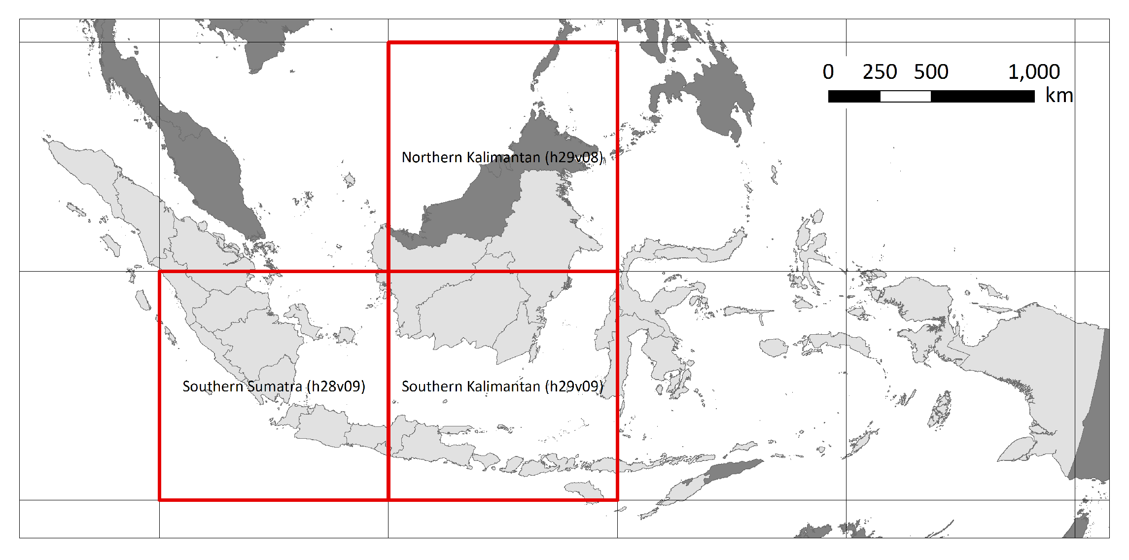
2.2. Study Region
2.3. Training Data
2.3.1. Tree Plantation Dataset
2.3.2. RSPO Dataset
3. Method
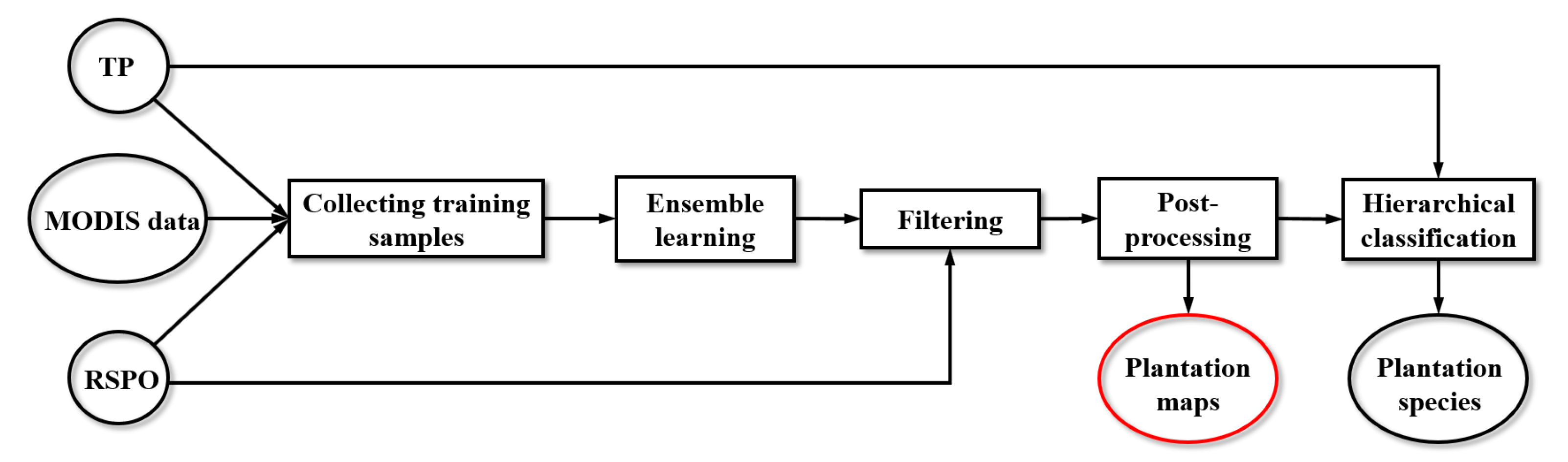
3.1. PALM Framework
3.1.1. Ensemble Learning Method
3.1.2. Collecting Training Samples
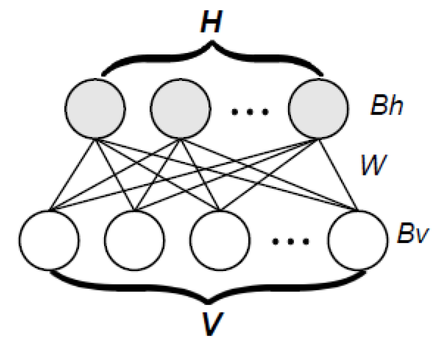
3.1.3. Learning Model
3.1.4. Filtering
3.1.5. Post-Processing
3.1.6. Hierarchical Classification
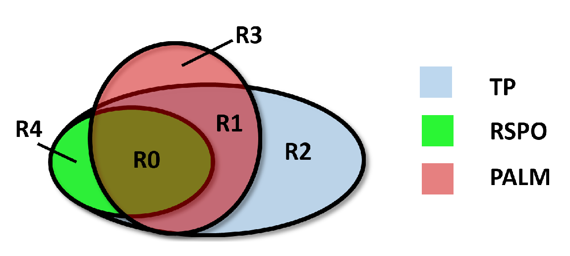
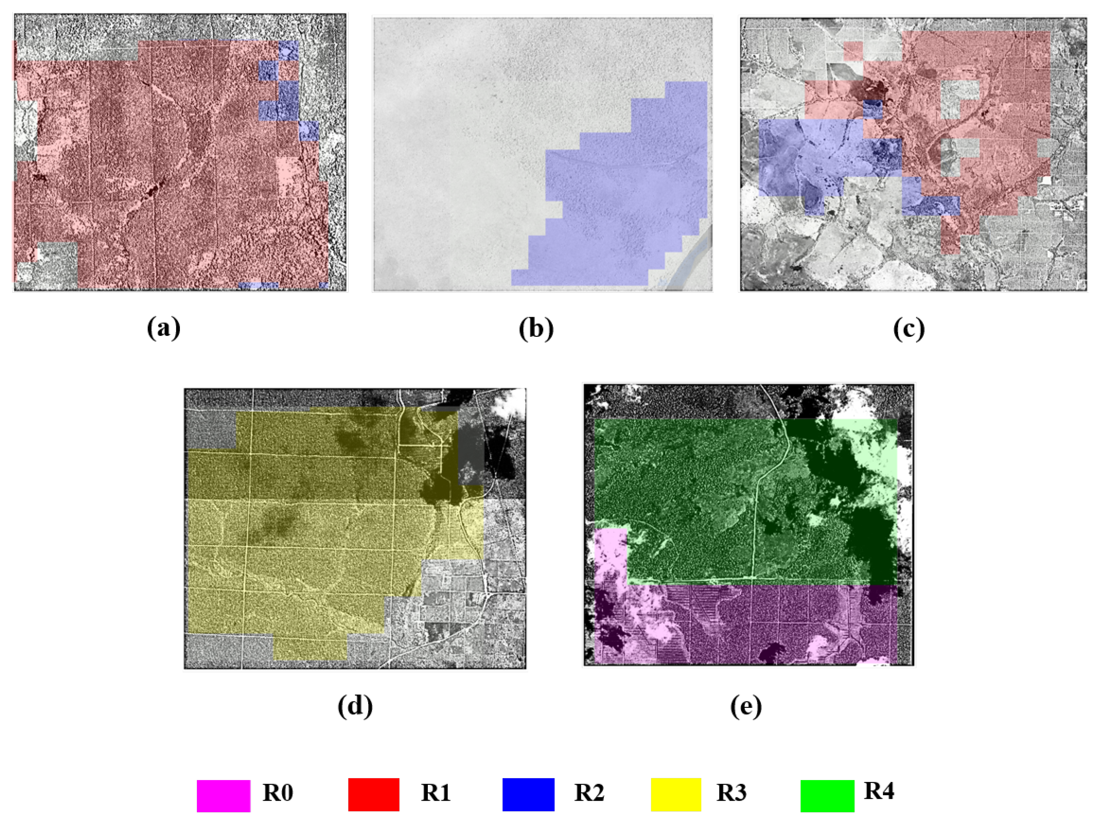
3.2. Validation of Plantation Maps
- R0—locations labeled as plantations by PALM, TP, and RSPO.
- R1—locations labeled as plantations by PALM and TP, but not by RSPO.
- R2—locations labeled as plantations by TP, but not by PALM and RSPO.
- R3—locations labeled as plantations by PALM, but not by TP. This includes both the locations detected by RSPO and the locations not detected by RSPO. Only a few locations in R3 are detected by RSPO.
- R4—locations labeled as plantations by RSPO, but not by PALM. This includes both the locations detected by TP and the locations not detected by TP.
4. Results
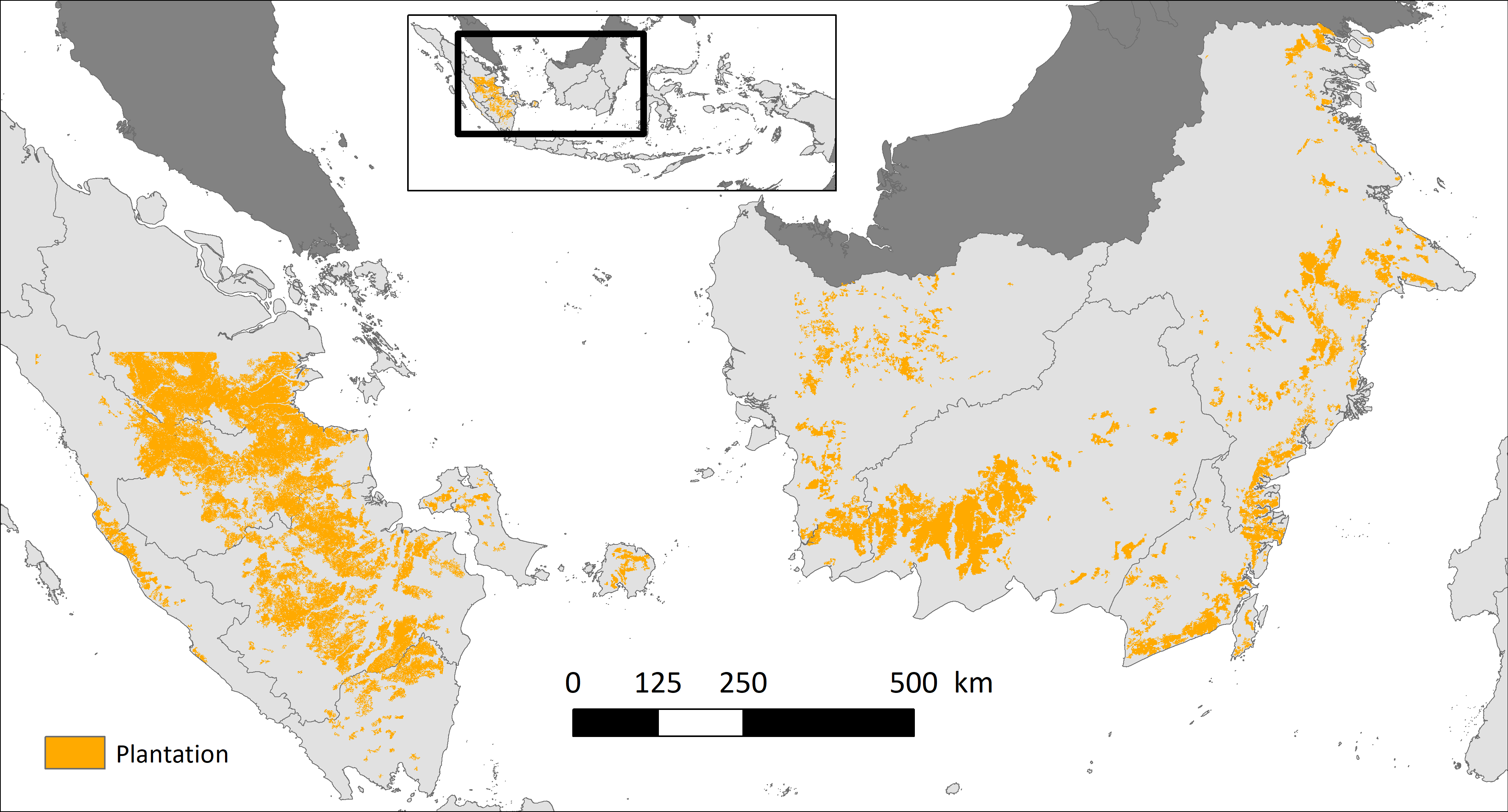
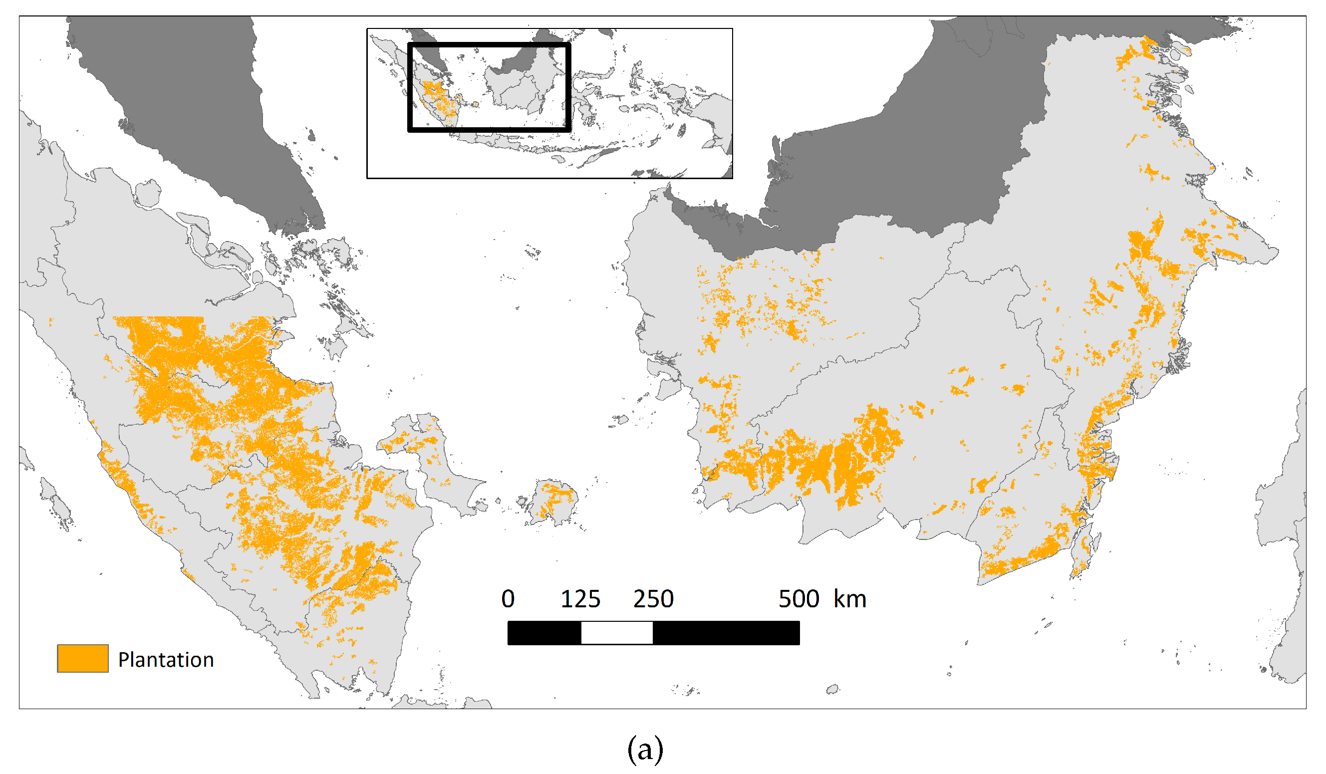
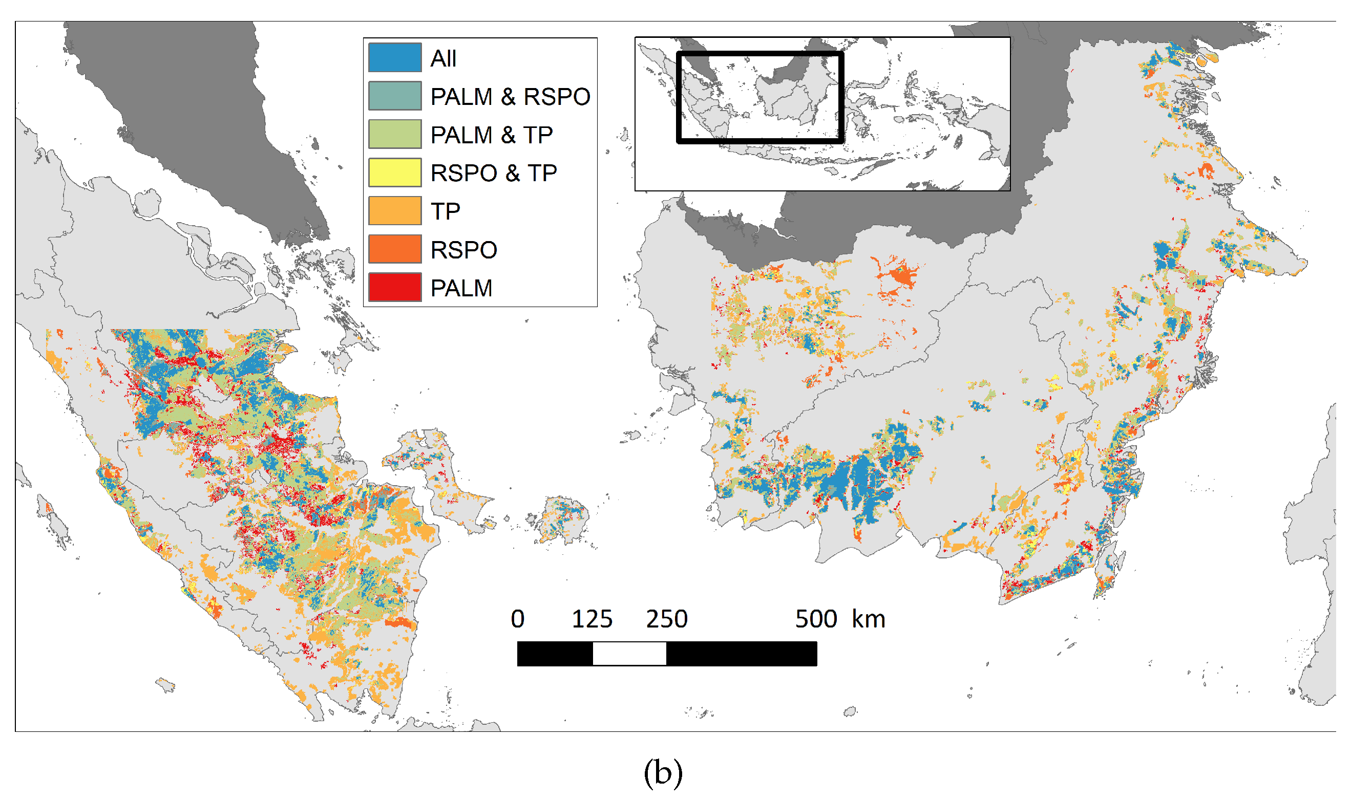
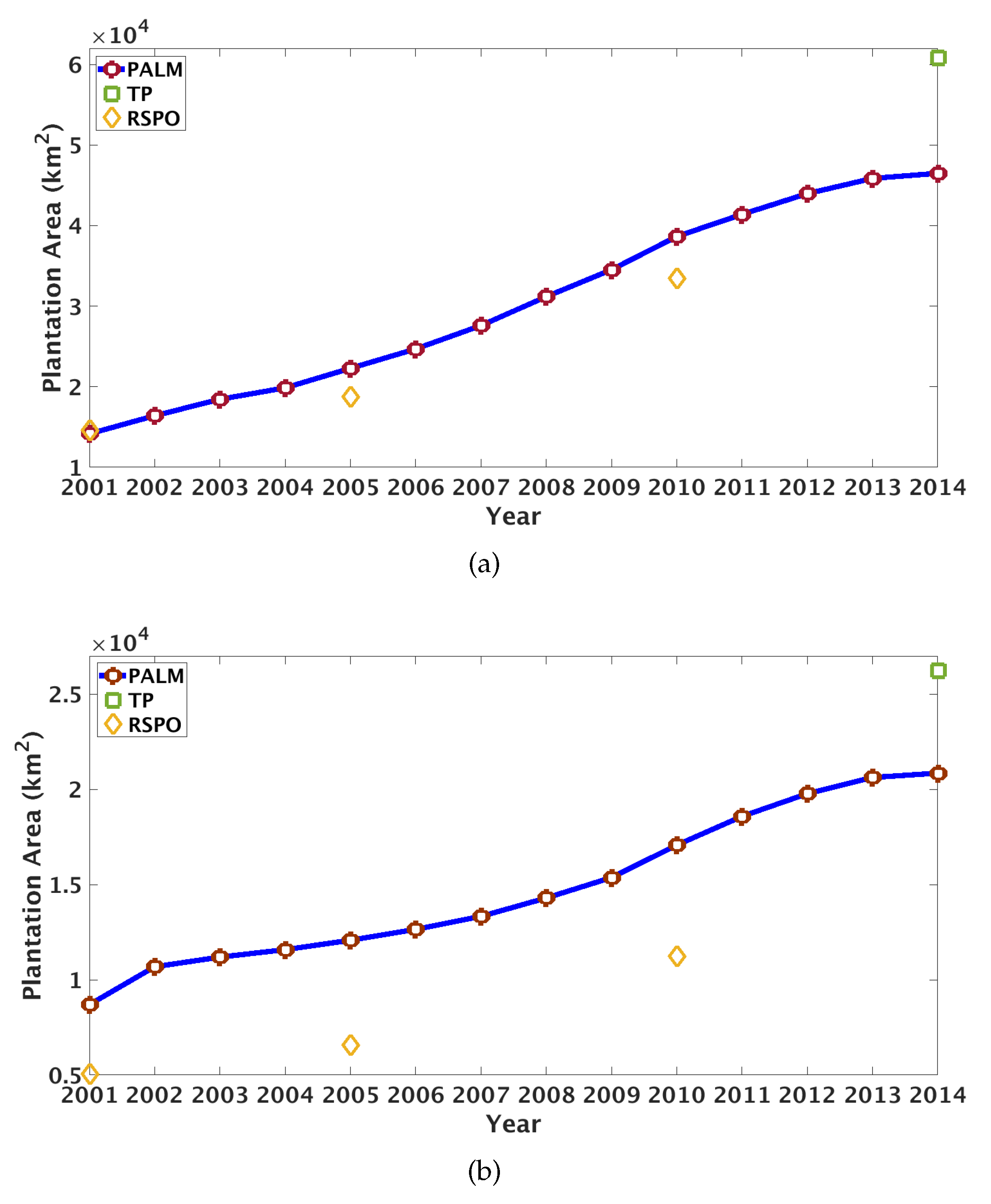
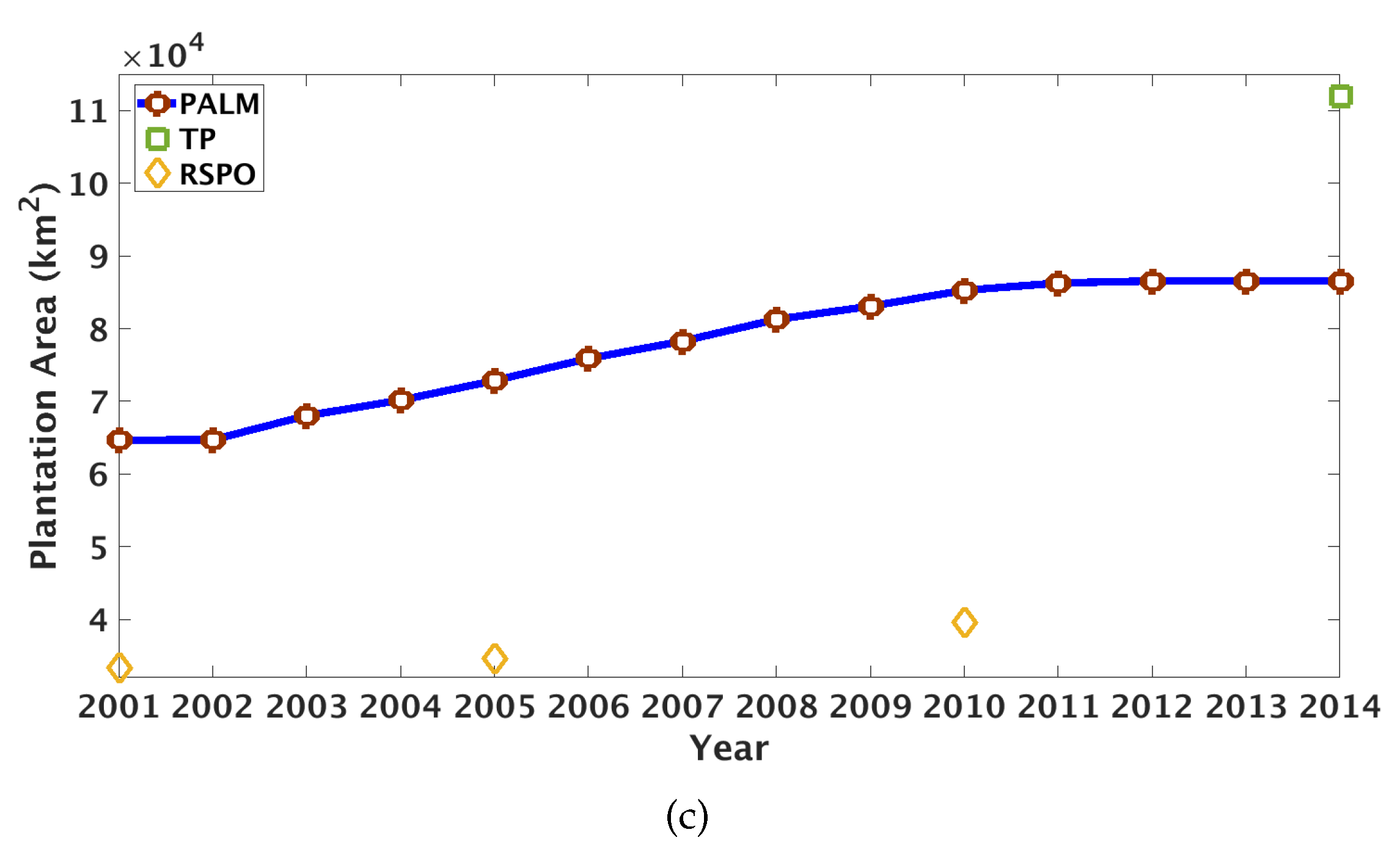
4.1. Plantation Map and Basic Statistics
4.2. Validation Using High-Resolution Images
4.2.1. Validation for Producer’s Accuracy
4.2.2. Validation for User’s Accuracy
4.2.3. Overall Accuracy
4.2.4. Case Studies of Model Performance
5. Discussion
5.1. Smallholder Tree Plantations
5.2. Tree Plantation Species-Specific Mapping
5.3. Classification Model
5.4. Limitations
6. Conclusions
Author Contributions
Funding
Acknowledgments
Conflicts of Interest
References
- Gaveau, D.L.; Sheil, D.; Salim, M.A.; Arjasakusuma, S.; Ancrenaz, M.; Pacheco, P.; Meijaard, E. Rapid conversions and avoided deforestation: Examining four decades of industrial plantation expansion in Borneo. Sci. Rep. 2016, 6, 1–13. [Google Scholar] [CrossRef] [PubMed]
- Ziegler, A.D.; Fox, J.M.; Xu, J. The rubber juggernaut. Science 2009, 324, 1024–1025. [Google Scholar] [CrossRef] [PubMed]
- Carlson, K.M.; Curran, L.M.; Asner, G.P.; Pittman, A.M.; Trigg, S.N.; Adeney, J.M. Carbon emissions from forest conversion by Kalimantan oil palm plantations. Nat. Clim. Chang. 2013, 3, 283. [Google Scholar] [CrossRef]
- Carlson, K.M.; Gerber, J.S.; Mueller, N.D.; Herrero, M.; MacDonald, G.K.; Brauman, K.A.; Havlik, P.; O’Connell, C.S.; Johnson, J.A.; Saatchi, S.; et al. Greenhouse gas emissions intensity of global croplands. Nat. Clim. Chang. 2017, 7, 63. [Google Scholar] [CrossRef]
- Wilcove, D.S.; Koh, L.P. Addressing the threats to biodiversity from oil-palm agriculture. Biodivers. Conserv. 2010, 19, 999–1007. [Google Scholar] [CrossRef]
- Carlson, K.M.; Curran, L.M.; Ponette-González, A.G.; Ratnasari, D.; Lisnawati, N.; Purwanto, Y.; Brauman, K.A.; Raymond, P.A. Influence of watershed-climate interactions on stream temperature, sediment yield, and metabolism along a land use intensity gradient in Indonesian Borneo. J. Geophys. Res. Biogeosci. 2014, 119, 1110–1128. [Google Scholar] [CrossRef]
- Samberg, L.H.; Gerber, J.S.; Ramankutty, N.; Herrero, M.; West, P.C. Subnational distribution of average farm size and smallholder contributions to global food production. Environ. Res. Lett. 2016, 11, 124010. [Google Scholar] [CrossRef]
- West, P.C.; Gibbs, H.K.; Monfreda, C.; Wagner, J.; Barford, C.C.; Carpenter, S.R.; Foley, J.A. Trading carbon for food: Global comparison of carbon stocks vs. crop yields on agricultural land. Proc. Natl. Acad. Sci. USA 2010, 107, 19645–19648. [Google Scholar] [CrossRef] [Green Version]
- Scarlat, N.; Dallemand, J.F. Recent developments of biofuels/bioenergy sustainability certification: A global overview. Energy Policy 2011, 39, 1630–1646. [Google Scholar] [CrossRef]
- Lambin, E.F.; Gibbs, H.K.; Heilmayr, R.; Carlson, K.M.; Fleck, L.C.; Garrett, R.D.; de Waroux, Y.l.P.; McDermott, C.L.; McLaughlin, D.; Newton, P.; et al. The role of supply-chain initiatives in reducing deforestation. Nat. Clim. Chang. 2018, 8, 109–116. [Google Scholar] [CrossRef]
- Schouten, G.; Glasbergen, P. Creating legitimacy in global private governance: The case of the Roundtable on Sustainable Palm Oil. Ecol. Econ. 2011, 70, 1891–1899. [Google Scholar] [CrossRef]
- Gunarso, P.; Hartoyo, M.E.; Agus, F.; Killeen, J.T.; Goon, J. Roundtable on Sustainable Palm Oil, Kuala Lumpur, Malaysia; Reports from the Technical Panels of the 2nd Greenhouse Gas Working Group of the Roundtable on Sustainable Palm Oil; 2013; Available online: https://rspo.org/publications/download/a2ac85181ed4501 (accessed on 1 February 2018).
- Moser, C.; Hildebrandt, T.; Bailis, R. International sustainability standards and certification. In Sustainable Development of Biofuels in Latin America and the Caribbean; Springer: New York, NY, USA, 2014; pp. 27–69. [Google Scholar]
- Sloan, S. Indonesia’s moratorium on new forest licenses: An update. Land Use Policy 2014, 38, 37–40. [Google Scholar] [CrossRef]
- Carlson, K.M.; Heilmayr, R.; Gibbs, H.K.; Noojipady, P.; Burns, D.N.; Morton, D.C.; Walker, N.F.; Paoli, G.D.; Kremen, C. Effect of oil palm sustainability certification on deforestation and fire in Indonesia. Proc. Natl. Acad. Sci. USA 2018, 115, 121–126. [Google Scholar] [CrossRef] [PubMed] [Green Version]
- Program, W.C.S.I. Oil Palm, Biodiversity and Indonesian Law; WCS Indonesia Programme: Bogor, Indonesia, 2010. [Google Scholar]
- Wakker, E.; Asia, A. Indonesia: Illegalities in Forest Clearance for Large-Scale Commercial Plantations; Forest Trends: Washington, DC, USA; Aidenvironment: Amsterdam, The Netherlands, 2014. [Google Scholar]
- Hansen, M.C.; Potapov, P.V.; Moore, R.; Hancher, M.; Turubanova, S.; Tyukavina, A.; Thau, D.; Stehman, S.; Goetz, S.; Loveland, T.; et al. High-resolution global maps of 21st-century forest cover change. Science 2013, 342, 850–853. [Google Scholar] [CrossRef] [Green Version]
- Hansen, M.C.; Stehman, S.V.; Potapov, P.V.; Loveland, T.R.; Townshend, J.R.; DeFries, R.S.; Pittman, K.W.; Arunarwati, B.; Stolle, F.; Steininger, M.K.; et al. Humid tropical forest clearing from 2000 to 2005 quantified by using multitemporal and multiresolution remotely sensed data. Proc. Natl. Acad. Sci. USA 2008, 105, 9439–9444. [Google Scholar] [CrossRef] [Green Version]
- Margono, B.A.; Turubanova, S.; Zhuravleva, I.; Potapov, P.; Tyukavina, A.; Baccini, A.; Goetz, S.; Hansen, M.C. Mapping and monitoring deforestation and forest degradation in Sumatra (Indonesia) using Landsat time series data sets from 1990 to 2010. Environ. Res. Lett. 2012, 7, 034010. [Google Scholar] [CrossRef]
- Rudorff, B.F.T.; Aguiar, D.A.; Silva, W.F.; Sugawara, L.M.; Adami, M.; Moreira, M.A. Studies on the rapid expansion of sugarcane for ethanol production in São Paulo State (Brazil) using Landsat data. Remote Sens. 2010, 2, 1057–1076. [Google Scholar] [CrossRef] [Green Version]
- Rudorff, B.F.T.; Adami, M.; Aguiar, D.A.; Moreira, M.A.; Mello, M.P.; Fabiani, L.; Amaral, D.F.; Pires, B.M. The soy moratorium in the Amazon biome monitored by remote sensing images. Remote Sens. 2011, 3, 185–202. [Google Scholar] [CrossRef] [Green Version]
- Fan, H.; Fu, X.; Zhang, Z.; Wu, Q. Phenology-based vegetation index differencing for mapping of rubber plantations using Landsat OLI data. Remote Sens. 2015, 7, 6041–6058. [Google Scholar] [CrossRef] [Green Version]
- Morel, A.C.; Saatchi, S.S.; Malhi, Y.; Berry, N.J.; Banin, L.; Burslem, D.; Nilus, R.; Ong, R.C. Estimating aboveground biomass in forest and oil palm plantation in Sabah, Malaysian Borneo using ALOS PALSAR data. For. Ecol. Manag. 2011, 262, 1786–1798. [Google Scholar] [CrossRef]
- Tropek, R.; Sedláček, O.; Beck, J.; Keil, P.; Musilová, Z.; Šímová, I.; Storch, D. Comment on “High-resolution global maps of 21st-century forest cover change”. Science 2014, 344, 981. [Google Scholar] [CrossRef] [PubMed] [Green Version]
- Koh, L.P.; Miettinen, J.; Liew, S.C.; Ghazoul, J. Remotely sensed evidence of tropical peatland conversion to oil palm. Proc. Natl. Acad. Sci. USA 2011, 108, 5127–5132. [Google Scholar] [CrossRef] [PubMed] [Green Version]
- Miettinen, J.; Hooijer, A.; Shi, C.; Tollenaar, D.; Vernimmen, R.; Liew, S.C.; Malins, C.; Page, S.E. Extent of industrial plantations on Southeast Asian peatlands in 2010 with analysis of historical expansion and future projections. Gcb Bioenergy 2012, 4, 908–918. [Google Scholar] [CrossRef] [Green Version]
- Miettinen, J.; Shi, C.; Tan, W.J.; Liew, S.C. 2010 land cover map of insular Southeast Asia in 250-m spatial resolution. Remote Sens. Lett. 2012, 3, 11–20. [Google Scholar] [CrossRef]
- Petersen, R.; Goldman, E.; Harris, N.; Sargent, S.; Aksenov, D.; Manisha, A.; Esipova, E.; Shevade, V.; Loboda, T.; Kuksina, N.; et al. Mapping Tree Plantations with Multispectral Imagery: Preliminary Results for Seven Tropical COUNTRIES; World Resources Institute: Washington, DC, USA, 2016. [Google Scholar]
- Miettinen, J.; Shi, C.; Liew, S.C. Land cover distribution in the peatlands of Peninsular Malaysia, Sumatra and Borneo in 2015 with changes since 1990. Glob. Ecol. Conserv. 2016, 6, 67–78. [Google Scholar] [CrossRef] [Green Version]
- Margono, B.A.; Usman, A.B.; Sugardiman, R.A. Indonesia’s forest resource monitoring. Indones. J. Geogr. 2016, 48, 7. [Google Scholar] [CrossRef]
- Jia, X.; Khandelwal, A.; Gerber, J.; Carlson, K.; West, P.; Kumar, V. Learning large-scale plantation mapping from imperfect annotators. In Proceedings of the IEEE International Conference on Big Data (Big Data), Washington, DC, USA, 5–8 December 2016; pp. 1192–1201. [Google Scholar]
- Gutiérrez-Vélez, V.H.; DeFries, R. Annual multi-resolution detection of land cover conversion to oil palm in the Peruvian Amazon. Remote Sens. Environ. 2013, 129, 154–167. [Google Scholar] [CrossRef]
- Dong, J.; Xiao, X.; Sheldon, S.; Biradar, C.; Xie, G. Mapping tropical forests and rubber plantations in complex landscapes by integrating PALSAR and MODIS imagery. Isprs J. Photogramm. Remote. Sens. 2012, 74, 20–33. [Google Scholar] [CrossRef]
- Tabassian, M.; Ghaderi, R.; Ebrahimpour, R. Combination of multiple diverse classifiers using belief functions for handling data with imperfect labels. Expert Syst. Appl. 2012, 39, 1698–1707. [Google Scholar] [CrossRef]
- Li, Z.; Fox, J.M. Mapping rubber tree growth in mainland Southeast Asia using time-series MODIS 250 m NDVI and statistical data. Appl. Geogr. 2012, 32, 420–432. [Google Scholar] [CrossRef]
- Friedman, J.H. On bias, variance, 0/1—loss, and the curse-of-dimensionality. Data Min. Knowl. Discov. 1997, 1, 55–77. [Google Scholar] [CrossRef]
- Jia, X.; Li, S.; Zhao, H.; Kim, S.; Kumar, V. Towards Robust and Discriminative Sequential Data Learning: When and How to Perform Adversarial Training? In Proceedings of the 25th ACM SIGKDD International Conference on Knowledge Discovery & Data Mining, Anchorage, AK, USA, 4–8 August 2019. [Google Scholar]
- Melgani, F.; Bruzzone, L. Classification of hyperspectral remote sensing images with support vector machines. IEEE Trans. Geosci. Remote Sens. 2004, 42, 1778–1790. [Google Scholar] [CrossRef] [Green Version]
- Bargiel, D. A new method for crop classification combining time series of radar images and crop phenology information. Remote Sens. Environ. 2017, 198, 369–383. [Google Scholar] [CrossRef]
- Jakimow, B.; Griffiths, P.; van der Linden, S.; Hostert, P. Mapping pasture management in the Brazilian Amazon from dense Landsat time series. Remote Sens. Environ. 2017. [Google Scholar] [CrossRef]
- Peuquet, D.J. Making space for time: Issues in space-time data representation. Geoinformatica 2001, 5, 11–32. [Google Scholar] [CrossRef]
- Ahlqvist, O. Extending post-classification change detection using semantic similarity metrics to overcome class heterogeneity: A study of 1992 and 2001 US National Land Cover Database changes. Remote Sens. Environ. 2008, 112, 1226–1241. [Google Scholar] [CrossRef]
- Zhu, Z.; Yang, L.; Stehman, S.V.; Czaplewski, R.L. Accuracy assessment for the US Geological Survey regional land-cover mapping program: New York and New Jersey region. Photogramm. Eng. Remote Sens. 2000, 66, 1425–1438. [Google Scholar]
- Ka, Z.; Olson, C. Using Multi-dimensional Scaling Technique To Examine The Similarity Among Land Cover Types. In Proceedings of the 10th Annual International Symposium on Geoscience and Remote Sensing, College Park, MD, USA, 20–24 May 1990; pp. 925–928. [Google Scholar]
- Karpatne, A.; Khandelwal, A.; Boriah, S.; Kumar, V. Predictive learning in the presence of heterogeneity and limited training data. In Proceedings of the 2014 SIAM International Conference on Data Mining, Philadelphia, PA, USA, 24–26 April 2014; pp. 253–261. [Google Scholar]
- Karpatne, A.; Jiang, Z.; Vatsavai, R.R.; Shekhar, S.; Kumar, V. Monitoring land-cover changes: A machine-learning perspective. IEEE Geosci. Remote Sens. Mag. 2016, 4, 8–21. [Google Scholar] [CrossRef]
- Vermote, E.; Kotchenova, S.; Ray, J. MODIS Land Surface Reflectance Science Computing Facility, MODIS Surface Reflectance User’s Guide, version 1.4; NASA: Greenbelt, MD, USA, 2015. [Google Scholar]
- Data Pool, LP DAAC, NASA Land Data Products and Services. Available online: https://lpdaac.usgs.gov/data_access/data_pool (accessed on 1 February 2018).
- Statistics Indonesia. Available online: https://www.bps.go.id/dynamictable/2015/09/04%2000\protect\kern+.2222em\relax00\protect\kern+.2222em\relax00/838/luas-tanaman-perkebunan-menurutpropinsi-dan-jenis-tanaman-indonesia-000-ha-2011-2016-.html (accessed on 7 July 2018).
- Abood, S.A.; Lee, J.S.H.; Burivalova, Z.; Garcia-Ulloa, J.; Koh, L.P. Relative contributions of the logging, fiber, oil palm, and mining industries to forest loss in Indonesia. Conserv. Lett. 2015, 8, 58–67. [Google Scholar] [CrossRef] [Green Version]
- Sagi, O.; Rokach, L. Ensemble learning: A survey. Wiley Interdiscip. Rev. Data Min. Knowl. Discov. 2018, 8. [Google Scholar] [CrossRef]
- Karpatne, A.; Kumar, V. Building Predictive Models for Noisy and Heterogeneous Data: An Application in Global Monitoring of Inland Water Dynamics. In Proceedings of the 2015 IEEE International Conference on Data Mining Workshop (ICDMW), Atlantic City, NJ, USA, 14–17 November 2015; pp. 1530–1531. [Google Scholar]
- Rodriguez-Galiano, V.F.; Ghimire, B.; Rogan, J.; Chica-Olmo, M.; Rigol-Sanchez, J.P. An assessment of the effectiveness of a random forest classifier for land-cover classification. ISPRS J. Photogramm. Remote Sens. 2012, 67, 93–104. [Google Scholar] [CrossRef]
- Chen, Y.; Lin, Z.; Zhao, X.; Wang, G.; Gu, Y. Deep learning-based classification of hyperspectral data. IEEE J. Sel. Top. Appl. Earth Obs. Remote Sens. 2014, 7, 2094–2107. [Google Scholar] [CrossRef]
- Glorot, X.; Bordes, A.; Bengio, Y. Domain adaptation for large-scale sentiment classification: A deep learning approach. In Proceedings of the 28th international conference on machine learning (ICML-11), Bellevue, DC, USA, 28 June 2011; pp. 513–520. [Google Scholar]
- Jia, X.; Willard, J.; Karpatne, A.; Read, J.; Zwart, J.; Steinbach, M.; Kumar, V. Physics guided RNNs for modeling dynamical systems: A case study in simulating lake temperature profiles. In Proceedings of the 2019 SIAM International Conference on Data Mining, Calgary, AL, Canada, 2–4 May 2019; pp. 558–566. [Google Scholar]
- Jia, X.; Khandelwal, A.; Nayak, G.; Gerber, J.; Carlson, K.; West, P.; Kumar, V. Incremental dual-memory lstm in land cover prediction. In Proceedings of the 23rd ACM SIGKDD International Conference on Knowledge Discovery and Data Mining, ACM, Halifax, NS, Canada, 13–17 August 2017; pp. 867–876. [Google Scholar]
- Jia, X.; Khandelwal, A.; Nayak, G.; Gerber, J.; Carlson, K.; West, P.; Kumar, V. Predict land covers with transition modeling and incremental learning. In Proceedings of the 2017 SIAM International Conference on Data Mining, Houston, FL, USA, 27–29 April 2017; pp. 171–179. [Google Scholar]
- Bengio, Y.; Lamblin, P.; Popovici, D.; Larochelle, H. Greedy layer-wise training of deep networks. In Proceedings of the Advances in Neural Information Processing Systems, Vancouver, BC, Canada, 3 December 2007; pp. 153–160. [Google Scholar]
- Read, J.S.; Jia, X.; Willard, J.; Appling, A.P.; Zwart, J.A.; Oliver, S.K.; Karpatne, A.; Hansen, G.J.; Hanson, P.C.; Watkins, W.; et al. Process-guided deep learning predictions of lake water temperature. Water Resour. Res. 2019, 55, 9173–9190. [Google Scholar] [CrossRef] [Green Version]
- Jia, X.; Khandelwal, A.; Carlson, K.; Gerber, J.S.; West, P.C.; Kumar, V. Plantation mapping in Southeast Asia. Front. Big Data 2019, 2, 46. [Google Scholar] [CrossRef] [Green Version]
- Nasrabadi, N.M. Pattern recognition and machine learning. J. Electron. Imag. 2007, 16, 049901. [Google Scholar]
- Sun, Y.; Wong, A.K.; Kamel, M.S. Classification of imbalanced data: A review. Int. J. Pattern Recognit. Artif. Intell. 2009, 23, 687–719. [Google Scholar] [CrossRef]
- Hinton, G.E. A practical Guide to training restricted Boltzmann machines. In Neural Networks: Tricks of the Trade; Springer: Berlin/Heidelberg, Germany, 2012; pp. 599–619. [Google Scholar]
- Hinton, G.E.; Osindero, S.; Teh, Y.W. A fast learning algorithm for deep belief nets. Neural Comput. 2006, 18, 1527–1554. [Google Scholar] [CrossRef]
- Welch, L.R. Hidden Markov models and the Baum-Welch algorithm. IEEE Inf. Theory Soc. Newsl. 2003, 53, 10–13. [Google Scholar]
- Forney, G.D. The viterbi algorithm. Proc. IEEE 1973, 61, 268–278. [Google Scholar] [CrossRef]
- Garrett, R.D.; Carlson, K.M.; Rueda, X.; Noojipady, P. Assessing the potential additionality of certification by the Round table on Responsible Soybeans and the Roundtable on Sustainable Palm Oil. Environ. Res. Lett. 2016, 11, 045003. [Google Scholar] [CrossRef]
- Padilla, M.; Stehman, S.V.; Chuvieco, E. Validation of the 2008 MODIS-MCD45 global burned area product using stratified random sampling. Remote Sens. Environ. 2014, 144, 187–196. [Google Scholar] [CrossRef]
- Indonesia Kicks off Scheme for Palm Oil Farmers to Meet New Sustainability Standards. Available online: http://www.undp.org/content/undp/en/home/presscenter/pressreleases/2015/02/24/indonesia-kicks-off-scheme-for-palm-oil-farmers-to-meet-new-sustainability-standards.html (accessed on 13 May 2018).
- Indonesia, Central Bureau of Statistics (BPS), The Abdul Latif Jameel Poverty Action Lab. Available online: https://www.povertyactionlab.org/partners/indonesia-central-bureau-statistics-bps (accessed on 13 May 2018).
- Commodity Prices–Price Charts, Data, and News–IndexMundi. Available online: https://www.indexmundi.com/commodities/ (accessed on 13 May 2018).
- Pohl, C. Mapping Palm Oil Expansion Using SAR to Study the IMPACT on the CO2 Cycle; IOP Publishing: Bristol, UK, 2014; Volume 20, p. 012012. [Google Scholar]
- Hu, J.; Mou, L.; Schmitt, A.; Zhu, X.X. FusioNet: A two-stream convolutional neural network for urban scene classification using PolSAR and hyperspectral data. In Proceedings of the 2017 Joint Urban Remote Sensing Event (JURSE), Dubai, UAE, 6–8 March 2017; pp. 1–4. [Google Scholar]
- LeCun, Y.; Bengio, Y.; Hinton, G. Deep learning. Nature 2015, 521, 436. [Google Scholar] [CrossRef] [PubMed]
- Liaw, A.; Wiener, M. Classification and regression by randomForest. News 2002, 2, 18–22. [Google Scholar]
- Freund, Y.; Schapire, R.; Abe, N. A short introduction to boosting. J. Jpn. Soc. Artif. Intell. 1999, 14, 1612. [Google Scholar]
- Heaton, J. An empirical analysis of feature engineering for predictive modeling. In Proceedings of the SoutheastCon 2016, Norfolk, VA, USA, 30 March–3 April 2016; pp. 1–6. [Google Scholar]
- Long, P.M.; Servedio, R.A. Random classification noise defeats all convex potential boosters. Mach. Learn. 2010, 78, 287–304. [Google Scholar] [CrossRef] [Green Version]
- Long, J.; Shelhamer, E.; Darrell, T. Fully convolutional networks for semantic segmentation. In Proceedings of the IEEE conference on computer vision and pattern recognition, Araucano Park, Chile, 11–18 December 2015; pp. 3431–3440. [Google Scholar]
- Noh, H.; Hong, S.; Han, B. Learning deconvolution network for semantic segmentation. In Proceedings of the IEEE International Conference on Computer Vision, Araucano Park, Chile, 11–18 December 2015; pp. 1520–1528. [Google Scholar]
- Timelapse–Google Earth Engine. Available online: https://earthengine.google.com/timelapse/ (accessed on 20 May 2018).


| Tile | Region | Study Area (km2) | MODIS Pixels |
|---|---|---|---|
| h29v09 | Southern Kalimantan | 328,028 | 1,312,112 |
| h29v08 | Northern Kalimantan | 262,386 | 1,049,546 |
| h28v09 | Southern Sumatra | 309,474 | 1,237,895 |
| Aggregated | High-Level Class | RSPO Land Cover Type | Description |
|---|---|---|---|
| Plantation | Oil palm | Oil Palm Plantation | Large industrial estates planted with oil palm |
| Plantation | Timber plantation | Timber Plantation | Large industrial estates planted to timber or pulp species |
| Plantation | Agriculture | Rubber Plantation | Large/medium sized industrial estates planted to rubber |
| Other | Agriculture | Coastal Fish Pond | Permanently flooded open areas |
| Other | Agriculture | Dry Cultivated Land | Herbaceous vegetation managed for row crops/pasture |
| Other | Agriculture | Mixed Tree Crops | Mosaic of cultivated and fallow land |
| Other | Agriculture | Rice Fields | Rice paddy with seasonal or permanent inundation |
| Other | Built-up | Settlements | Villages, urban areas, industrial areas, open mining |
| Other | Mining | Mining | Open area with surface mining activities |
| Other | Bare soil | Upland Grassland | Open vegetation dominated by grasses |
| Other | Bare soil | Upland Shrub land | Open woody vegetation, including forest and grassland |
| Other | Bare soil | Swamp Grassland | Extensive cover of herbaceous plants with shrubs/trees |
| Other | Bare soil | Swamp Shrub land | Open woody vegetation on poorly drained soils |
| Other | Water body | Water Bodies | Rivers, streams and lakes |
| Other | Disturbed forest | Disturbed Mangrove | Forest of mangrove species with evidence of clearing |
| Other | Disturbed forest | Disturbed Swamp Forest | Swamp forest with evidence of logging and clearings |
| Forest | Disturbed forest | Disturbed Upland Forest | Basal area reduced significantly due to logging |
| Forest | Undisturbed forest | Undisturbed Upland Forest | Natural forest, highly diverse species and high basal area |
| Forest | Undisturbed forest | Undisturbed Swamp Forest | Natural forest with temporary or permanent inundation |
| Full Name | Land Cover | 2000 | 2005 | 2010 | A2000 | A2005 | A2010 |
|---|---|---|---|---|---|---|---|
| Coastal Fish Pond | CFP | 5120 | 5159 | 6324 | 1.28 | 1.29 | 1.58 |
| Rubber Plantation | CPL | 18398 | 19813 | 19741 | 4.60 | 4.95 | 4.94 |
| Dry Cultivated Land | DCL | 44640 | 57555 | 86230 | 11.16 | 14.39 | 21.56 |
| Disturbed Upland Forest | DIF | 413561 | 404786 | 386326 | 103.39 | 101.20 | 96.58 |
| Disturbed Mangrove | DIM | 6731 | 6731 | 6500 | 1.68 | 1.68 | 1.63 |
| Disturbed Swamp Forest | DSF | 81790 | 83001 | 66836 | 20.45 | 20.75 | 16.71 |
| Upland Grassland | GRS | 14772 | 12026 | 12273 | 3.69 | 3.01 | 3.07 |
| Mining | MIN | 1249 | 2308 | 4168 | 0.31 | 0.58 | 1.04 |
| Mixed Tree Crops | MTC | 6944 | 7657 | 7995 | 1.74 | 1.91 | 2.00 |
| Oil Palm Plantation | OPL | 27948 | 42572 | 101806 | 6.99 | 10.64 | 25.45 |
| Rice Fields | RCF | 28697 | 29416 | 30419 | 7.17 | 7.35 | 7.60 |
| Upland Shrub land | SCH | 288002 | 294930 | 258922 | 72.00 | 73.73 | 64.73 |
| Settlements | SET | 2776 | 2839 | 2840 | 0.69 | 0.71 | 0.71 |
| Swamp Grassland | SGR | 16713 | 13887 | 13525 | 4.18 | 3.47 | 33.8 |
| Swamp Shrub land | SSH | 98669 | 103509 | 108240 | 24.67 | 25.88 | 27.06 |
| Timber Plantation | TPL | 12008 | 12531 | 12117 | 3.00 | 3.13 | 3.03 |
| Undisturbed Upland Forest | UDF | 136217 | 115656 | 97007 | 34.05 | 28.91 | 24.25 |
| Undisturbed Swamp Forest | USF | 88069 | 77928 | 71035 | 22.02 | 19.48 | 17.76 |
| Water Bodies | WAB | 19808 | 19808 | 19808 | 4.95 | 4.95 | 4.95 |
| Species | 2001 | 2002 | 2003 | 2004 | 2005 | 2006 | 2007 | 2008 | 2009 | 2010 | 2011 | 2012 | 2013 | 2014 |
|---|---|---|---|---|---|---|---|---|---|---|---|---|---|---|
| Acacia | 2.96 | 2.96 | 3.95 | 4.46 | 5.20 | 5.87 | 6.62 | 7.33 | 7.97 | 8.46 | 8.91 | 9.26 | 9.62 | 9.62 |
| Rubber | 0.41 | 0.41 | 0.66 | 0.84 | 1.04 | 1.23 | 1.50 | 1.95 | 2.42 | 2.92 | 3.53 | 3.78 | 4.24 | 4.24 |
| Oil Palm | 4.76 | 5.38 | 7.24 | 8.48 | 10.45 | 12.42 | 14.78 | 17.78 | 20.63 | 23.87 | 26.29 | 27.89 | 30.04 | 31.05 |
| Species | 2001 | 2002 | 2003 | 2004 | 2005 | 2006 | 2007 | 2008 | 2009 | 2010 | 2011 | 2012 | 2013 | 2014 |
|---|---|---|---|---|---|---|---|---|---|---|---|---|---|---|
| Oil Palm | 8.19 | 10.18 | 10.69 | 11.08 | 12.05 | 12.61 | 13.32 | 14.29 | 15.26 | 17.07 | 18.08 | 19.17 | 20.12 | 20.44 |
| Species | 2001 | 2002 | 2003 | 2004 | 2005 | 2006 | 2007 | 2008 | 2009 | 2010 | 2011 | 2012 | 2013 | 2014 |
|---|---|---|---|---|---|---|---|---|---|---|---|---|---|---|
| Acacia | 9.30 | 9.32 | 9.91 | 10.37 | 11.01 | 11.78 | 12.31 | 12.70 | 13.14 | 13.75 | 14.07 | 14.19 | 14.19 | 14.19 |
| Coconut | 9.54 | 9.54 | 9.85 | 10.06 | 10.27 | 10.50 | 10.64 | 10.82 | 10.97 | 11.13 | 11.21 | 11.23 | 11.23 | 11.23 |
| Rubber | 17.24 | 17.24 | 18.24 | 18.69 | 19.14 | 19.79 | 20.47 | 21.65 | 21.98 | 22.34 | 22.53 | 22.49 | 22.54 | 22.55 |
| Oil Palm | 28.58 | 28.59 | 30.03 | 31.03 | 32.40 | 33.80 | 34.84 | 36.09 | 36.98 | 38.05 | 38.46 | 38.59 | 38.59 | 38.60 |
| Region | Sampled Locations | True Plantations | PALM Plantations | TP Plantations | RSPO Plantations |
|---|---|---|---|---|---|
| Southern Kalimantan | 1116 | 951 | 890 (93.59%) | 864 (90.85%) | 751 (78.97%) |
| Northern Kalimantan | 1004 | 724 | 578 (79.83%) | 626 (86.46%) | 388 (53.59%) |
| Southern Sumatra | 1030 | 872 | 702 (80.50%) | 744 (85.32%) | 221 (25.34%) |
| Metric | R0 | R1 | R2 | R3 | R4 |
|---|---|---|---|---|---|
| number of pixels | 85,539 | 71,801 | 77,916 | 25,790 | 13,471 |
| confidence | 100% | 81.87% | 39.00% | 42.86% | 41.90% |
| Metric | R0 | R1 | R2 | R3 | R4 |
|---|---|---|---|---|---|
| number of pixels | 20,984 | 31,220 | 48,567 | 11,408 | 4948 |
| confidence | 100% | 81.65% | 26.37% | 58.33% | 37.40% |
| Metric | R0 | R1 | R2 | R3 | R4 |
|---|---|---|---|---|---|
| number of pixels | 60,488 | 210,037 | 169,565 | 67,795 | 16,256 |
| confidence | 100% | 84.16% | 31.98% | 53.77% | 48.33% |
| MODIS Tile | Region | PALM | TP | RSPO |
|---|---|---|---|---|
| h29v09 | Southern Kalimantan | 85.53% | 72.51% | 92.10% |
| h29v08 | Northern Kalimantan | 85.93% | 57.83% | 88.04% |
| h28v09 | Southern Sumatra | 82.59% | 65.59% | 89.06% |
| MODIS Tile | Region | PALM | TP | RSPO |
|---|---|---|---|---|
| h29v09 | Southern Kalimantan | 97.15% | 93.04% | 96.48% |
| h29v08 | Northern Kalimantan | 97.70% | 94.22% | 95.77% |
| h28v09 | Southern Sumatra | 88.35% | 81.31% | 60.88% |
| - | Entire study region | 94.29% | 89.35% | 84.03% |
| MODIS Tile | Region | PALM | TP | RSPO |
|---|---|---|---|---|
| h29v09 | Southern Kalimantan | 0.9616 | 0.8948 | 0.9547 |
| h29v08 | Northern Kalimantan | 0.9738 | 0.9126 | 0.9521 |
| h28v09 | Southern Sumatra | 0.7236 | 0.4472 | −0.0275 |
| - | Entire study region | 0.9149 | 0.8220 | 0.7622 |
© 2020 by the authors. Licensee MDPI, Basel, Switzerland. This article is an open access article distributed under the terms and conditions of the Creative Commons Attribution (CC BY) license (http://creativecommons.org/licenses/by/4.0/).
Share and Cite
Jia, X.; Khandelwal, A.; Carlson, K.M.; Gerber, J.S.; West, P.C.; Samberg, L.H.; Kumar, V. Automated Plantation Mapping in Southeast Asia Using MODIS Data and Imperfect Visual Annotations. Remote Sens. 2020, 12, 636. https://doi.org/10.3390/rs12040636
Jia X, Khandelwal A, Carlson KM, Gerber JS, West PC, Samberg LH, Kumar V. Automated Plantation Mapping in Southeast Asia Using MODIS Data and Imperfect Visual Annotations. Remote Sensing. 2020; 12(4):636. https://doi.org/10.3390/rs12040636
Chicago/Turabian StyleJia, Xiaowei, Ankush Khandelwal, Kimberly M. Carlson, James S. Gerber, Paul C. West, Leah H. Samberg, and Vipin Kumar. 2020. "Automated Plantation Mapping in Southeast Asia Using MODIS Data and Imperfect Visual Annotations" Remote Sensing 12, no. 4: 636. https://doi.org/10.3390/rs12040636