Extending Landsat 8: Retrieval of an Orange contra-Band for Inland Water Quality Applications
by
 , , , , and
Alexandre Castagna
1,* ,
,
Stefan Simis
2 ,
,
Heidi Dierssen
3 ,
,
Quinten Vanhellemont
4,
Koen Sabbe
1 and
Wim Vyverman
1 1
Protistology and Aquatic Ecology, Ghent University, Krijgslaan 281, 9000 Gent, Belgium
2
Plymouth Marine Laboratory, Prospect Place, The Hoe, Plymouth PL1 3DH, UK
3
Department of Marine Science, University of Connecticut, Groton, CT 06340, USA
4
Royal Belgian Institute of Natural Sciences, Operational Directorate Natural Environments, Vautierstraat 29, 1000 Brussels, Belgium
*
Author to whom correspondence should be addressed.
Remote Sens. 2020, 12(4), 637; https://doi.org/10.3390/rs12040637
Submission received: 17 January 2020
/
Revised: 11 February 2020
/
Accepted: 12 February 2020
/
Published: 14 February 2020
(This article belongs to the Special Issue Lake Remote Sensing)
Abstract
:The Operational Land Imager (OLI) onboard Landsat 8 has found successful application in inland and coastal water remote sensing. Its radiometric specification and high spatial resolution allows quantification of water-leaving radiance while resolving small water bodies. However, its limited multispectral band set restricts the range of water quality parameters that can be retrieved. Identification of cyanobacteria biomass has been demonstrated for sensors with a band centered near 620 nm, the absorption peak of the diagnostic pigment phycocyanin. While OLI lacks such a band in the orange region, superposition of the available multispectral and panchromatic bands suggests that it can be calculated by a scaled difference. A set of 428 in situ spectra acquired in diverse lakes in Belgium and The Netherlands was used to develop and test an orange contra-band retrieval algorithm, achieving a mean absolute percentage error of 5.39% and a bias of −0.88% in the presence of sensor noise. Atmospheric compensation error propagated to the orange contra-band was observed to maintain about the same magnitude (13% higher) observed for the red band and thus results in minimal additional effects for possible base line subtraction or band ratio algorithms for phycocyanin estimation. Generality of the algorithm for different reflectance shapes was tested against a set of published average coastal and inland Optical Water Types, showing robust retrieval for all but relatively clear water types (Secchi disk depth > 6 m and chlorophyll a mg m). The algorithm was further validated with 79 matchups against the Ocean and Land Colour Imager (OLCI) orange band for 10 globally distributed lakes. The retrieved band is shown to convey information independent from the adjacent bands under variable phycocyanin concentrations. An example application using Landsat 8 imagery is provided for a known cyanobacterial bloom in Lake Erie, US. The method is distributed in the ACOLITE atmospheric correction code. The contra-band approach is generic and can be applied to other sensors with overlapping bands. Recommendations are also provided for development of future sensors with broad spectral bands with the objective to maximize the accuracy of possible spectral enhancements.
1. Introduction
The typical spatial resolution of 250 m to 1 km offered by dedicated polar orbiting Ocean Colour (OC) sensors is often insufficient to fully resolve processes occurring in coastal, transitional and inland waters [1,2,3]. For inland waters, underrepresentation of small or narrow water bodies is substantial, with most systems unresolved at those moderate resolutions [1,4,5]. The requirement of higher spatial resolution has led to the development of water applications for sensors originally designed for terrestrial remote sensing [6,7,8], the most relevant of which are the Landsat and Sentinel-2 series. The sensors on those platforms offer global coverage at high spatial resolution (10–60 m) and feature near infrared (NIR) and shortwave infrared (SWIR) bands appropriate for atmospheric correction over turbid waters [7,9]. However, they feature fewer and broader multispectral (MS) bands in the visible range than the standard OC sensors, limiting the variety of algorithms that can be applied, and hence the water quality parameters that can be retrieved.
The Operational Land Imager (OLI) on Landsat 8 resolves four visible bands covering the deep-blue (435–451 nm), blue (452–512 nm), green (533–590 nm) and red (636–673 nm) and has found successful application for remote sensing of water quality (e.g., transparency, dissolved organic carbon and algal biomass [10,11,12]). This waveband configuration, however, does not allow retrieval of direct information related to phycocyanin (PC) abundance, a diagnostic pigment for the presence of cyanobacteria which are a major concern in eutrophic inland waters. Cyanobacterial blooms are an increasingly frequent phenomenon, and can produce noxious and toxic compounds that cause health risks to wildlife and humans, as well as taste and odor problems in drinking water [13,14]. The presence of an orange band (∼620 nm) covering the PC absorption peak has allowed specific semi-empirical and semi-analytical algorithms to be developed for cyanobacteria detection [15]. Recent examples are the algorithms developed for the OC sensor Medium Resolution Imaging Spectrometer (MERIS) [16,17,18,19] and its follow-on, the Ocean and Land Colour Instrument (OLCI). At present, high spatial resolution orange bands are only available on commercial sensors, notably the imagers on WorldView-2 and -3 (DigitalGlobe) and on the SuperDove constellation (Planet Labs Inc.).
Previous studies have found a high level of redundancy in the spectral information of the water leaving signal [20,21,22] and have shown that reconstruction of hyperspectral data is possible from a small number of narrow wavebands (typically 5–15) using multilinear regression. This spectral redundancy in a setting of broad adjacent wavebands could result that information in the orange spectral region is redundant for the OLI band set, being completely contained in the adjacent green and red MS bands. However, for an accurate and site-transferable prediction of spectral data, the wavebands must be located at key central wavelengths in order to capture most of the independent spectral information (e.g., [23]). Therefore, this method may not be appropriate for the orange spectral region over water bodies that can experience cyanobacterial blooms. PC shows no universal correlation with other major pigments [17] and its absorption shape shows minimal superposition with the adjacent green and red OLI bands [24]. As a consequence, orange band spectral reconstruction and indirect PC retrievals with OLI will depend on local correlations that may not be transferable to other sites or hold in time [25]. Indeed, the presence of independent information in the orange spectral region in environments experiencing cyanobacterial blooms led to the recent recommendations of inclusion of an orange band for future satellite missions of water quality [1,2].
In addition to the visible bands, OLI features a high spatial resolution (15 m) panchromatic (Pan) band spanning green to red wavelengths (503–676 nm). Pan bands are commonly used in remote sensing applications to resolve features at higher spatial resolution than provided in the MS channels, made possible due to the wider spectral integration. The high spatial information of the Pan band is merged with the spectral information of the MS bands in a process referred to as Pan sharpening, producing a final image with the highest possible spatial resolution [26]. Considering that the Pan band covers the full spectral range of the green and red MS bands, we propose to use the Pan band not to enhance spatial information, but to enhance spectral information. The objective is to extract a virtual orange (590–635 nm) band—or contra-band—from the Pan band, offsetting its signal against the green and red MS bands. This approach can potentially extract additional spectral information not captured in the correlation structure with neighboring bands. To our knowledge, this is the first application of the Pan band to derive a new virtual spectral channel. We hypothesize that the orange contra-band has potential to significantly expand the application of OLI/Landsat 8 in water quality research [1,2]. Routine retrieval of this band through implementation in atmospheric correction software can provide an unprecedented open-access global dataset of orange reflectance at high spatial resolution. Additionally, the theoretical basis and general framework of contra-band algorithms is developed to support application to other sensors and provide guidance on how to maximize its retrieval accuracy and potential independent information content in the design of future sensors.
2. Theory
The normalized spectral response function (SRF) of band x, , describes the spectral integration performed by the sensor assembly of spectral radiance, , into the discrete waveband radiance . Mathematically, this integration can be decomposed into a sum of the integrals of n component spectral subregions:
where is the wavelength range of waveband x, and the wavelength subsets of each i spectral subregion. Equation (1a) is valid as long as the regions do not overlap and their collection completely covers the original SRF spectral range. We can take advantage of this decomposition to extract additional spectral information from a system of overlapping bands.
We can apply this concept to OLI, by dividing the Pan band into four regions, delimited by the boundaries of the Full Width at Half Maximum (FWHM) of the green and red MS bands (Figure 1B). As a consequence of this definition, the scaled radiances from Regions 2 and 4 are approximately equal to the radiance from the green and red MS bands, respectively. Therefore, a contra-band containing the combined radiance from regions 1 (turquoise, 503–533 nm) and 3 (orange, 590–635 nm) can be retrieved analytically by:
where the analytical scaling coefficients S are found by solving Equation (2b). The derivation of Equation (2) and its generalization for a system of n bands is provided in Appendix A. The analytical retrieval results in negligible error (Section S1 of Supplementary Materials), related to small differences in the spectral weighting profile between the MS bands and the equivalent Pan regions. The retrieved composite band, however, combines spectral information of different optically active water constituents and optical processes. For example, Region 1 receives stronger influence from detrital and dissolved organic absorption than Region 3. It is therefore necessary to isolate the information of those two regions.
The superposition of the defined regions with the spectral mass specific in vivo absorption coefficient of pigment groups, , the mass specific absorption coefficient of Non-Algal Particles (NAP), , and a relative magnitude of absorption coefficient by chromophoric dissolved organic matter (CDOM), , is presented in Figure 1B. It shows that Region 1 is in the green gap of chlorophyll (Chl) pigments, dominated by carotenoids, while Region 3 includes the PC peak, the smaller red Chl a absorption peak and Chl c. It can be expected that Region 3 will present larger independent variation from Regions 2 (green) and 4 (red) than Region 1, in particular for turbid inland waters, where different phytoplankton groups may have strong presence of accessory photosynthetic pigments. Region 1 is not strongly affected by pigments but will be correlated with signals from adjacent bands due to particle scattering in addition to carotenoids, inorganic and organic absorption (particulate and dissolved). If this correlation is sufficiently high, signal from the turquoise region can be accounted for within acceptable errors, allowing for robust isolation of the orange signal.
Based on the correlation structure with the adjacent MS bands, the signal from the turquoise region can be accounted for explicitly, by using spectral reconstruction [20] to estimate and adding a turquoise term to Equation (2a). The turquoise signal can also be accounted for implicitly, maintaining the structural relation of Equation (2a), but solving directly for by substituting the analytical scaling coefficients with empirical ones calculated by multilinear regression. The explicit and implicit approaches are similar provided that the same MS bands are used, but the single step algorithm of the implicit approach will have a gain in statistical performance by incorporating the Pan band directly into the regression.
To gain the covariance necessary to estimate and remove the signal from the turquoise region, the variable atmospheric and surface signals are removed by specifying the generic radiances to be the water-leaving radiances defined immediately above the water surface, . Further increase in covariance is achieved with the normalization of the by the downwelling plane irradiance, . Those normalized radiances are commonly referred to as remote sensing reflectance, (sr). The theory leading to Equation (2b) is only approximate in reflectance space (cf. Appendix A), but the gain in covariance by using reflectances when the turquoise signal estimation is necessary outweighs the added uncertainty of the approximation. By substitution and algebraic simplification of Equation (2a), the implicit approach is functionally described by:
where the coefficients carry information on the scaling and proportionality of the MS and Pan bands and the orange signal contained in the Pan band.
3. Data and Methods
3.1. Analysis
The validity of the proposed relation between Pan and MS bands and subsequent retrieval of the orange contra-band was evaluated with a diverse in situ dataset of 428 hyperspectral collected over Dutch and Belgian lakes. In situ hyperspectral data were converted into equivalent OLI wavebands, as described in Section 3.2. Regression analysis of Equation (3) was performed with Ordinary Least Squares (OLS) based on a random subsample of half the in situ dataset, and validated with the complementary set. To retrieve a robust set of coefficients and performance statistics, and describe their uncertainties, the procedure was repeated 10,000 times over unique random subsets of the dataset. We further evaluated the error propagation of sensor noise using the OLI average signal to noise ratio (SNR) and top of atmosphere (TOA) radiances over water targets [29,30]. Average clear skies , described below, were used to convert radiance noise into equivalent noise. Independent random deviates from Gaussian noise distributions of each band were generated for each spectrum and the procedure repeated 10,000 times to evaluate retrieval performance.
Clear skies were calculated with a combination of the transmittance for the direct component [31] and the model of Zibordi and Voss [32] for the diffuse component and are described elsewhere [33]. The model was run for Sun zenith angles of 20–70 in steps of 10 and for wavelengths between 350 and 750 nm in steps of 10 nm. The range of Sun zenith angles was chosen to match the Sun zenith angles range of the average OLI TOA radiances described by [29]. The optical properties of four standard aerosol models were retrieved for three levels of relative humidity (50%, 80% and 95%) and two aerosol loads representing an aerosol optical thickness at 550 nm, , of 0.1 and 0.2. The surface reflectivity used for the sky radiance distribution calculation was modeled as a combination of Fresnel reflectance for an isotropic incident radiance over a flat surface and a Lambertian water-leaving reflectance representing mesotrophic waters. For all simulations, the molecular atmosphere composition was set to 2.5 cm of precipitable water, 300 DU of ozone, 450 ppm of CO and a surface pressure of 101.25 KPa. The average of the 168 simulations was used as average clear sky .
The error propagation of spectrally correlated error caused by imperfect atmospheric compensation (AC) [34] was also evaluated. The AC additive error is dependent on local atmospheric and surface conditions, illumination and observation geometry, availability of bands and the specific algorithm used for AC. Therefore, for a realistic simulation of AC error propagation, measured AC errors for OLI processed with the ACOLITE AC code [6,9,35,36] were used (Figure 2). Those AC errors were taken from Vanhellemont [36], calculated by contrasting 98 matchups between OLI-ACOLITE estimated with in situ observations from 14 coastal and 2 lacustrine AERONET-OC sites [37], the majority of which are located in the US and Europe. OLI scenes were processed with the Dark Spectrum Fitting (DSF) algorithm and compared against Level 2.0 AERONET-OC observations. ACOLITE was chosen to implement AC for the Pan band and provide an application demonstration (described below). The error for OLI-ACOLITE in the sites studied by Vanhellemont [36] ranged from −0.0054 sr to 0.0046 sr, with a median of 0.0005 sr. Those additive errors represent 0.14% to 759.7% of the red band signal of our in situ data, with a median of 7.47%. Since the Pan band AC error is not available, it was calculated as the average of the red and green band errors. The matchups between OLI-ACOLITE and AERONET-OC are provided in the Supplementary Materials.
To evaluate the generality of the coefficients fitted with the in situ dataset, the retrieval was applied to the standardized spectra of the Optical Water Types (OWT) cluster averages [38]. The OWT clusters were based on the LIMNADES dataset and representative of inland and coastal waters in a wide geographical set [38]. Specifically, the nine coastal (C) and thirteen inland (I) waters cluster averages were used.
To further evaluate the algorithm performance under realistic conditions and for different lakes, the OLI orange contra-band was compared with the OLCI orange band for a set of 10 globally distributed lakes (Table 1). These lakes were chosen based on online reports of occasional cyanobacterial blooms (e.g., CyanoTRACKER [39]) and for their geographical distribution. The comparison of the absolute magnitude between OLI and OLCI requires that atmospheric effects are removed and that AC errors be equal for both sensors. Therefore, the AC scheme was specifically designed to force the same median AC errors for each matchup, by assuming that the atmosphere is spatially constant over the scene at each acquisition time and that the pixel scale is constant in the time difference between the sensors acquisitions. Compensation for atmosphere effects is challenging over turbid inland waters in the absence of SWIR bands, thus OLI processed with ACOLITE was taken as reference for the multispectral bands other than the orange. OLCI imagery was first partially compensated for Rayleigh effects only with SeaDAS [40] (version 7.5.3) and then subtracted by the scene median difference to OLI multispectral bands. The OLCI orange band (620 nm) was subtracted by the spline interpolated median difference from green and red bands. Before the median difference calculation, OLI imagery was aggregated to 300 m and linear regressions based on in situ data were used to bandshift OLI to equivalent OLCI signal. The process results in zero scene median difference between bandshifted OLI and OLCI in the multispectral bands other than the orange, while observed median differences in between the sensors will reflect real differences between the bands. In total, 133 matchups over the period of three years (mid 2016–2019) were used for the cross-validation. Only scenes with low fractional coverage of clouds, Sun zenith angle lower than 65 and observed within 1 h difference between the sensors were used. To ensure that the assumptions of spatially constant atmosphere and spatiotemporally constant reflectance were met to a good approximation, pixels with a reflectance ratio at 442 nm % of the median value were masked and matchups only processed if at least 10% of water pixels were not masked. The 442 nm band is suitable because its relative SRF is nearly equivalent for both sensors. This criterion will remove regions with significant atmospheric heterogeneity and constrain the influence of moving cloud shadows, advection and changes in the vertical profile of cyanobacteria occurring in the time between the overpasses. This quality control step yielded 79 matchups (Table 1).
The presence of new information in the orange band, that is, information not already present in the correlation structure of the adjacent MS bands, was evaluated by comparing the residuals of the contra-band algorithm with those of an empirical spectral reconstruction based on multilinear regression to the green and red MS bands (). This empirical algorithm does not include a Pan band and represents an explicit assumption that all information in the orange region is contained in the adjacent spectral regions. Only the adjacent green and red MS bands were included, as would be recommended in real applications to prevent propagation of AC errors in the blue bands and adjacency effects in the NIR. The residuals of both algorithms were then regressed against the PC to Chl a ratio to explore possible bias. Finally, the potential application of the orange contra-band for water quality studies was demonstrated for an OLI scene acquired in western Lake Erie. A schematic representation of the analysis provided in the main text is presented in Figure 3. Statistics of performance were the coefficient of determination (), the Root Mean Squared Error (RMSE), the Mean Absolute Percentage Error (MAPE) and the bias, calculated as the mean percentage error. All analysis were performed in R version 3.3.3 [41].
3.2. In Situ Dataset
The inland water datasets used for algorithm development are described below. Application of the algorithm to additional oceanic and coastal spectra are presented in Section S2 of the Supplementary Materials.
3.2.1. Dutch Lakes
Measurements in Dutch lakes were performed throughout 2003 (Lake Loosdrecht) and during the growth season in 2004–2005 (Lake IJsselmeer) with detailed methodology described in [16,17]. Lake Loosdrecht (5.063E, 52.192N) is a shallow eutrophic lake, with a surface area of 9.8 km and average depth of 1.9 m. The lake is fully mixed with a prominent particulate detrital component and associated high turbidity (Secchi disk depth up to 0.5 m), favoring filamentous cyanobacteria which do not form surface accumulations, while Chl a concentrations reach 100 mg m. Lake IJsselmeer (5.338E, 52.812N) is the largest freshwater body in western Europe, with a surface area of 1190 km and an average depth of 4.4 m. The shallow depth and exposure to winds result in a typically well-mixed water column, albeit with marked horizontal gradients in turbidity and occasional resuspension of bottom sediments and surface accumulation of cyanobacteria. It is an eutrophic system, experiencing recurrent cyanobacterial blooms that peak towards the end of summer, with Chl a concentrations in near-surface accumulations reaching 300 mg m under calm conditions. The average Secchi disk depth is 0.8 m.
3.2.2. Belgian Lakes
Measurements in Belgian lakes were performed seasonally throughout 2017 (three lakes) and 2018 (four lakes), spanning a broad range of conditions. The Spuikom (2.953E, 51.227N) is a shallow coastal lagoon, with a surface area of 0.82 km and an average depth of 1.5 m. It experiences a cycle of diatom blooms in spring and transition to transparent waters in autumn, with extensive bottom coverage by macroalgae. It is subject to strong coastal winds that can cause sediment resuspension, adding bottom sediments and benthic diatoms to the water column. The Chl a concentration varies from 2 to 25 mg m, while Secchi disk depth ranges from 0.62 m to bottom. The Hazewinkel (4.392E, 51.066N) is a mesotrophic lake with an area of 0.66 km and a maximum depth of 20 m. It has a peak of phytoplankton abundance in spring, with Chl a reaching 20 mg m, after which the concentration stays fairly stable around 5 mg m. Secchi disk depth varies from 1 to 6 m. Submerged macrophytes are confined to near-shore locations due to a steep basin slope. The Donkmeer (3.980E, 51.037N) is the second largest lake in the Flanders region, with a surface area of 0.86 km and an average depth of 2 m. It experiences recurrent cyanobacterial blooms of Anabaena spp. and Planktothrix agardhii [42] from summer to autumn, reaching Chl a concentrations of 400 mg m and a Secchi disk depth of 0.2 m. Its northern and southern portions are connected through a narrow and shallow passage, with the northern portion experiencing a shorter period of cyanobacterial blooms due to management actions. The Dikkebus (2.844E, 50.818N; 0.36 km, 2.5 m deep) and Zillebeke (2.909E, 50.837N; 0.28 km, 2 m deep) are two lakes created in the 13th century for water supply, a function that remains to date along with recreational activities. Both lakes exhibit yearly blooms of Microcystis aeruginosa and Aphanizomenon flos-aquae [42], with Chl a varying from 10 to 105 mg m and Secchi disk depth from 0.5 to 2 m. Additional stations are included from four other lakes: the Bocht (4.389E, 51.073N; 0.35 km and 18 m deep), the Nieuwdonk (3.976E, 51.034N; 0.26 km and 22 m deep) and two unnamed adjacent lakes (4.028E, 51.101N; ≈0.16 km each and 10 m deep). All coordinates are relative to the WGS84 datum.
3.2.3. Radiometric Measurements
For both datasets, reflectances were calculated from radiances measured with portable, hand held spectrometers. For the campaigns in the Netherlands, a PR-650 (Photo Research, Inc., Chatsworth, CA, USA) with 1 Field of View (FOV) foreoptics was used. The instrument has 8 nm FWHM with a spectral sampling of 4 nm, covering the range from 380 to 780 nm. For the campaigns in Belgium, a HandHeld FieldSpec (Analytical Spectral Devices, Inc., Boulder, CO, USA) with 7.5 FOV foreoptics was used. The instrument has 3.6 nm FWHM and spectral sampling of 1.6 nm, covering the range from 325 to 1075 nm, but only data between 380 and 780 nm were used to match the wavelength range of the PR-650 spectrometer. For both datasets, was estimated from near-coincident measurements of the surface radiance of a Spectralon™ target, held parallel to the surface. In campaigns in the Netherlands, the classical above water approach was employed, where radiance from the water target was measured at 42 of nadir, with a relative azimuth of 90 to the Sun. Correction for the sky glint component was performed with a fixed surface reflectance factor of 0.029 applied to sky radiance measurement performed at 42 of zenith and equal relative azimuth [16,17]. For Belgian campaigns, reflectances were calculated with a variant of the sky-blocked approach (SBA) presented by Leeet al. [43], with detector foreoptics positioned 2.5 cm below the surface, 0.5 m from the inflatable boat and aligned in the Sun–boat plane. Platform and instrument shadowing correction were calculated with a Monte Carlo radiative transfer code (Castagna et al., in prep.). A sample of 20 spectra from each dataset is presented in Figure 4.
The corresponding OLI waveband were calculated using the average in band and out-of-band normalized SRF of OLI Focal Plane Modules [44], with waveband integration of spectral and as:
where the SRF is normalized such that its integral equals unity. Belgian campaigns used an uncalibrated radiometer, and, although calibration factors cancel out for reflectance calculation at full instrument resolution [45], when simulating another sensor band, the spectral calibration factors are inside the integrals of Equation (4) and strictly do not cancel out. To avoid introducing bias from the SRF weighting of the uncalibrated data (digital counts), the averaged simulated was used to calculate from the hyperspectral for OLI waveband calculation.
3.2.4. Pigment Concentration
Pigment data from the IJsselmeer were used to explore the sensitivity of different orange band retrievals to diagnostic cyanobacteria pigments. The dataset included High-Performance Liquid Chromatography (HPLC) following Rijstenbil [46] for organically soluble pigments and spectrophotometric analysis of phycobilipigments with a protocol modified from Sarada et al. [47]. Detailed information on pigment extraction methods is provided elsewhere [16,17]. In short, HPLC samples were concentrated on glass fiber filters, flash frozen in liquid nitrogen and stored at −80 C. Pigments were extracted in acetone using a bead beater and cleared by centrifugation. The HPLC used a reverse-phase column (Waters Nova-pak C18; Waters Millennium HPLC system) and detection was performed with fluorescence (Waters 474 Scanning Fluorescence Detector) and absorption (Waters 996 Photodiode Array Detector) detectors. Samples for phycobilipigments were concentrated by high-speed centrifugation, suspended in a phosphate buffer of pH 7.4, and frozen and thawed nine times at −20 C and room temperature (around 20 C), respectively, while kept in darkness. Phycobilipigment concentrations were quantified from the absorption spectra of supernatants of centrifuged samples, according to standard equations [48].
Pigment concentration of organically soluble pigments was also analyzed for Belgian lakes, with HPLC methods following Van Heukelem and Thomas [49]. Extraction was similar to the method used in the Dutch campaigns, except that sonication was used to break the cells and suspension was cleared by filtration through a 0.22 m syringe filter. The HPLC used a reverse-phase column (Eclipse XDB C) and detection was performed with spectral absorption (Agilent 1100 series, Diode Array Detector). The pigment analysis was used to describe the range of pigment concentration and their ratios (Table 2).
4. Results
4.1. Calibration and Validation of the Orange contra-Band Retrieval
The procedure of repeated analysis with different random subsets of data for calibration and validation allows using all available data for improved estimation of model parameters, while also providing insight into algorithm stability. The final retrieval algorithm, with slope coefficients calculated as the average of 10,000 fits and with their standard deviations (SD) reported in parentheses, was:
Similarly, the average and SD of the performance statistics were , % (%) and (±0.49%), for the RMSE, MAPE and bias, respectively. The application of the algorithm for the complete dataset is presented in Figure 5.
The dependency on the specific subsets of data used for calibration and validation is expressed through the SD and can be compared with the coefficient of variation (CV). For the Pan and green bands slope coefficients, CVs were %, while it reached 36% for the red band. This dependency is expected since the dataset was acquired over waters with variable levels of PC and Chl a, which share signals between the orange and red bands, providing variable relations depending on the concentration range of each random subsample of the dataset. Despite this variability, the RMSE and the MAPE showed not only small magnitudes but also were stable across the multiple subsets, with CVs %. Greater variability was observed for the bias with a CV of 52%, which was of little practical consequence due to its small magnitude (average −0.95%). The absence of an effect of the red band slope variability on the RSME and MAPE can be explained by the lower magnitude of the red reflectance and of the slope coefficient when compared to the other bands.
4.2. Sensitivity to Errors in the Input Data
While the small magnitude of the uncertainty statistics for the in situ data are encouraging, they are related to retrieval in a condition of negligible error in the input data when compared to data from spaceborne sensors. Even for accurately calibrated sensors, uncertainty is expected to arise from random sensor noise and spectrally correlated AC error.
The average values of over water targets are presented in Table 3, together with the SNR of the OLI sensor at average TOA radiance over water targets [30,50] and the calculated noise levels in equivalent units. When the independent random noise was added to the in situ data, the final performance as expressed by the RMSE, MAPE and bias were , and , respectively (Figure 6A).
Since AC errors are not inherent to the OLI sensor (in contrast to noise) or to the contra-band algorithm, propagation of AC error into the orange contra-band should be considered relative to AC errors in the MS bands. We chose the red band AC error to be used as a reference value for this comparison, since it is an adjacent band and for OLI-ACOLITE it presents the lowest average absolute AC error in the visible range. When the spectrally correlated errors from imperfect AC were applied, propagation of error into the orange contra-band was on average 13% higher than the respective error in the red MS band (Figure 6B). The relative AC error propagated in the orange contra-band is primarily a function of the red band AC error and secondarily a function of the spectral shape of the AC error in the green to red range, as evidenced by the green to red AC error difference, and can be described by .
4.3. Generality of the OLI Orange contra-Band Algorithm
The standardized OWT cluster averages used in this study are reproduced from Spyrakos et al. [38] in Figure 7A,B. The clustering of our in situ dataset with the OWT cluster averages showed that most inland water reflectance shapes were absent or underrepresented (Figure 7C). For coastal clusters, only Clusters C-4 and C-9 were represented. Despite the sub-optimal representation of global spectral shape diversity, application of the orange contra-band algorithm to the OWT averages results in a performance within algorithm uncertainty for eleven out of thirteen inland clusters and for three out of nine coastal clusters (Figure 7D). Larger than expected errors were found for Clusters I-3, I-13, C-1, C-2, C-3, C-6, C-7 and C-8, with Clusters I-3 and I-13 being approximately equivalent to Clusters C-6 and C-7, respectively. Those clusters represent relatively clear waters and blue-enhanced spectral shapes, with relatively high transparency (Secchi disk depth average > 6 m) and low Chl a concentration (average < 1.6 mg m [38]). The bias for those clusters arises from the empirical estimation of the turquoise signal from the reflectance in the green-red spectral region only, which is not able to accommodate all blue to green ratio range even when relatively blue-enhanced spectra are present in the calibration dataset (not shown). While a universal algorithm applicable to all spectral shapes is desirable, reflectance spectra in those clusters represent clear water conditions, to which the SNR of OLI is not adequate. Based on the spectral shapes of our in situ data and OWT cluster averages integrated with OLI normalized SRF, a blue to red band ratio > 2 must be used to flag input reflectance spectra for which significant bias is expected. This ratio is representative of the relative contribution of turquoise to orange signal in the Pan band. Additionally, based on and OLI , a sr threshold could be used to flag input reflectance spectra for which sensor random noise can be an important contributor to the recorded signal. The proposed algorithm threshold flags however will not capture optically shallow waters and errors will depend on the magnitude and shape of the benthic reflectance contribution to the water-leaving signal. Sections S2 and S3 of the Supplementary Materials further explore the suitability of the algorithm flags, the application of the current calibration of the OLI orange contra-band algorithm to blue-enhanced and optically shallow waters and the consequence of addition of the blue MS band together with blue-enhanced spectra in the calibration set. The proposed flags to identify spectra for which application is not recommended (blue-enhanced, low turbidity) are highlighted below:
4.4. Cross-Validation with OLCI/Sentinel-3 Imagery
The Sentinel-3 mission [51] was designed to provide quality optical data over water targets with the OLCI sensor, a medium resolution (300 m) multispectral sensor with 21 wavebands covering the visible to the NIR (388 to 1043 nm) and performing with SNR in the visible range under typical radiances over water targets [52]. The OLCI band set includes a 10 nm wide orange band centered at 620 nm that can be used for cross-validating the retrieved with the OLI orange contra-band and help to access the performance of the algorithm on spaceborne data over a diverse set of lakes.
The orange contra-band retrieval algorithm was implemented in the free and open source ACOLITE AC code [6,9,35,36] to provide its functionality in concert with atmospheric correction. The code was updated to include the AC of the OLI Pan band, allowing for the retrieval of and application of Equation (5). The OLCI AC scheme described in the methods is illustrated in Figure 8A and results in zero median difference of bandshifted and spatially aggregated OLI against OLCI in the multispectral bands other than the orange. The smooth atmospheric difference between Rayleigh corrected OLCI and ACOLITE-OLI is interpolated in the orange region with a spline function between the green and the red median differences. Since the OLCI is subtracted by an interpolated value, it is not forced to agree on its median value with the OLI orange contra-band and ratios on the processed data should represent real signal differences between the sensors. When data from all lakes were combined, the regression slope between the of OLCI and OLI was , with a MAPE of around the regression line (Figure 8B). A similar and consistent result was observed when the analysis was performed per lake (Figure 8C). The average ratio observed in the orbital imagery was consistent with expectations from the OWT cluster averages and our in situ data integrated with each waveband normalized SRFs. Due to the differences in waveband center wavelength and spectral width, the ratio of between the two sensors is expected to change depending on the spectral shape and was observed to vary between 0.85 and 0.99 in our in situ data (Figure 8D) and between 0.833 and 1.044 for the OWT cluster averages. Detailed analysis per lake and ancillary information are presented in Section S4 and Fugure S5 of the Supplementary Materials.
4.5. Contribution of New Information from the Orange contra-Band
The presence of independent information in the orange spectral region is the main justification to pursue an orange contra-band with OLI. In view of recent studies showing the redundancy of spectral information [21], quantifying the amount of independent waveband information is important, but not straightforward. It is expected that, for most spectra with pigment absorption dominated by Chl a and/or Chl c, the information content in the orange region will be completely contained in the red MS band. However, the increasing range of Chl b, PC and/or PE concentrations are expected to result in an increase of the amount of independent information contained in the orange region relative to the green and red bands (cf. Figure 1B).
The performance of an empirical spectral reconstruction algorithm that assumes that the orange information is contained in the adjacent green and red MS bands is shown in Figure 9A. It compared well with that of the contra-band algorithm retrieval (Figure 5). The variable auxiliary pigments concentration resulted in an increase of scatter, but with the MAPE for the in situ data increasing from ≈4% to only ≈6%. This result suggests that the correlation of the information content is high enough for on average accurate retrieval from MS bands alone. However, the average relation showed decreasing performance as the relative pigment composition of samples deviated from the average composition in the dataset. This behavior is clearly shown in Figure 9B, where residuals from both algorithms are regressed against the PC to Chl a ratio. When it is assumed that the information in the orange spectral region is redundant with green and red OLI MS bands, model residuals have larger variance and are more strongly anticorrelated with PC / Chl a. When PC is absent, larger under- or overestimation of can occur.
4.6. Example Application: Lake Erie Cyanobacteria Bloom
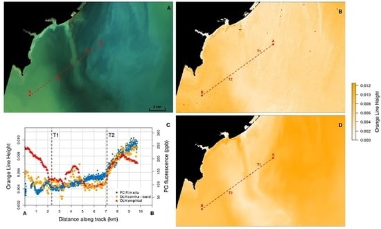
An OLI scene acquired in late August 2013 (23 August 2013 16:12:25Z) over west Lake Erie, US, shows high spatial heterogeneity in water color in the transition between the Maumee Bay (MB) waters and the Detroit River (DR) plume (Figure 10A). The scene was selected due to the availability of in situ data sampled one day before the image acquisition [53]. Bio-optical measurements, including PC fluorescence and particle scattering, were performed in a northeast to southwest transect with in water instrumentation [53] (Figure 10C). Cell counts from discrete samples show virtual absence of cyanobacteria in the DR waters but high abundance in MB.
The OLI image was processed to retrieve the orange reflectance line height (OLH) against a baseline calculated by linear interpolation of the green and red MS bands (Figure 10B,D). The OLH is a broadband application of the MERIS’ PC index (PCI) [54], a green–orange–red extension of the baseline algorithm proposed by Dekker [55]. The algorithm was designed to remove the influence of particle scattering and be proportional to PC concentration. Since proportionality with PC is site specific [15], our objective was to evaluate if the OLH calculated with the orange contra-band captures the spatial pattern of PC concentration. The OLH was retrieved both for the contra-band algorithm of Equation (5) (Figure 10B) and for the empirical spectral reconstruction algorithm that assumes that the information in the orange spectral range is contained in the adjacent green and red MS bands (Figure 10D). The OLH extracted for the transect line for both models is also shown in Figure 10C.
The comparison between the OLH retrieved with Equation (5) and the in situ PC fluorescence shows good qualitative agreement. Differences are mainly located within Kilometers 5–7 and were likely caused by the 24-h difference between in situ observation and imagery acquisition. The relative spread in the OLH transect and the granulated spatial texture are caused by the Pan band noise and possible spatial resampling artifacts, absent in the retrieval with the empirical spectral reconstruction algorithm, since it only includes the MS bands. However, this empirical algorithm underestimates the orange reflectance in the DR region, leading to overestimation of the OLH. The OLH magnitudes in the patch where field data show cyanobacteria to be absent are even higher than in the MB region, where the bloom was identified. This result shows in practice the large errors that can result if information in the orange spectral region is assumed to be contained in the adjacent bands.
5. Discussion
As presented in Section 2, additional spectral information can be obtained from any combination of overlapping bands. A purely analytical contra-band retrieval can be applied directly only if the set of conditions described in Appendix A are satisfied, at least to good approximation. OLI satisfies those conditions for the band set of green, red and Pan bands, and a composite band combining information from the turquoise and orange spectral regions can be retrieved with a MAPE of 0.4%, independent of spectral shape (Section S1, Supplementary Materials). If the short wavelength limit of the OLI Pan band more closely matched the short wavelength limit of the green MS band, an analytical retrieval of the orange contra-band would be possible with similar performance. While the conceptual analytical relation is kept, retrieval of the orange information is only possible if the turquoise signal is first estimated explicitly or implicitly, where the analytical scaling coefficients are substituted by empirical ones calculated with regression analysis. Under this condition, the MAPE of the retrieval in the absence of noise and AC error in the input data was 3.87%. When average noise levels expected over water targets are propagated through the algorithm, the average uncertainty increased to only 5.41%. Without the addition of the AC errors, this value can be compared with the Landsat 8 mission goal of maximum 3% uncertainty at TOA reflectances [56]. The lower performance stems particularly from the Pan band, with lower SNR than the MS bands and different spatial sampling. While the Pan band has double spatial resolution than the MS bands and in theory spatial aggregation necessary to match the resolution of the MS bands would lower the noise levels by half, possible resampling artifacts may compensate the gain in SNR. Those effects and their interaction were not included in the error propagation analysis.
Spectrally correlated errors from imperfect AC will further increase uncertainty, but our results show that, for realistic OLI-ACOLITE AC errors, the propagated error into the orange contra-band has the same direction and about the same magnitude (13% higher) as errors in the red MS band. This result is expected since the AC error in the Pan band will be approximately equal to the average of the errors in the green and red MS bands, compensating most of the spectral structure of the AC error. This is true as long as only the MS bands that overlap with the Pan band are included in the algorithm, as shown in practice with the Lake Erie example. When accounting for the turquoise signal, addition of the blue MS band can greatly improve performance for a larger set of OWTs (Section S3, Supplementary Materials). However, in the presence of random noise the propagated error increases due to the additional random error in the blue band. Even more important is the propagation of AC errors, with typical overestimation of (undercompensation of atmospheric effects) resulting in underestimation of . This result is an important example of the need to access algorithm performance in the presence of realistic sensor noise and AC error.
One component of uncertainty not directly addressed in this study, is the absolute calibration of the Pan band. Any bias in the Pan band calibration will be directly propagated to the orange contra-band. Pan band performance is periodically evaluated with standard methods also applied to the MS bands, including dark current, solar diffuser, calibration lamp and lunar readings [50]. Despite those efforts of performance evaluation, dedicated vicarious calibration efforts have shown that small adjustments are necessary to remove focal plane module dependent bias from MS bands [57]. Understandably, the Pan band was not included in those efforts due to the previous absence of its use for aquatic applications and the additional challenges of cross-calibrating it with concurrent ocean colour missions. However, recent per focal plane module gain factors calculated for the MS bands over water targets are lower than 1.5% [57] and it is reasonable to expect that maximum Pan bias will be at the same level. Indeed, the cross-validation exercise with OLCI imagery supports this expectation, with slope magnitude in the range observed for in situ data. We encourage future vicarious calibrations efforts to include the Pan band for evaluation.
Ultimately, the major source of uncertainty in the orange contra-band retrieval is related to the empirical dependency on the spectral shape of the to account for the turquoise signal. In our dataset, signals from the turquoise and orange spectral regions have approximately the same magnitude. Since the turquoise and orange spectral regions cover 16% and 26%, respectively, of the Pan band SRF area, the orange contribution to Pan signal will be higher than the turquoise contribution. Indeed, signal from the turquoise region represented of the Pan signal in our in situ data, while the signal from the orange region represented . It results that, for all except eight samples, the ratio of the orange to turquoise contribution for the Pan band signal was higher than 1, ranging from 0.86 to 4.11. This range overlaps in the higher end with the ratios for the OWT cluster averages (ranging from 0.03 to 4.32). It is worth noting that all OWT clusters averages for which we observed larger than predicted errors had a ratio lower than 1. The accuracy of the algorithm for different spectral shapes, however, is not directly dependent on those ratios.
As discussed in Section 4.2, it is possible to provide an accurate retrieval of for all average spectral shapes of the OWT clusters if the blue MS band is added to the algorithm together with calibration data including clear water spectra. Rather, the accuracy is dependent on the magnitude of the turquoise estimation error compared to the magnitude of the orange signal. With information only in the green to red spectral region it is not possible to provide a model for all the blue to red ratio variability in reflectance spectra of natural waters. Therefore, errors in the turquoise estimation will be acceptable only when a consistent subset of the blue to red spectral shapes are represented in the calibration dataset. The blue to red band ratio is the most representative ratio, considering the available MS bands, of the turquoise to orange relative contribution to the Pan band. While adding the blue MS band could provide the required free parameter for retrieval independent of spectral shape in an error free scenario, it will likewise increase the turquoise estimation error due to AC errors. Consequently, the current algorithm is a compromise between generality and accuracy. It includes only the overlapping bands to provide robustness to AC errors and includes only meso- to eutrophic waters in the calibration dataset to provide coefficients that are applicable to conditions when retrieval of an orange band is possible (SNR limitations) and desirable (possibility of cyanobacterial blooms). Application of the algorithm with the current coefficients is not recommended for relatively blue-enhanced waters (Section S2, Supplementary Materials), mostly represented by relatively low concentration of optically active components (e.g., Chl a< 1.6 mg m and Secchi disk depth > 6 m). The conditions where the algorithm is not expected to perform can be flagged by requiring a and possibly in combination with sr.
The empirical coefficients retrieved from our in situ dataset over lakes in Belgium and the Netherlands were directly applicable to most inland water spectral shapes represented in the LIMNADES dataset. This offers support that the orange contra-band can be used in algorithms for PC retrieval in a wide geographical and seasonal coverage. Additional support is offered by the matchup comparison between of OLI and OLCI spanning multiple lakes and seasonal stages, with variable turbidity and dominance of sediments or cyanobacteria. Nine out of ten lakes had ratios within the range expected from our in situ data (0.85–0.99). The exception was the Rybinsk Reservoir, with a ratio of 1.04. The observed MAPE of in the matchup analysis was larger than expected due to algorithm uncertainty and OLI noise alone. Although the AC method was proposed to remove AC error differences between the two sensors, residual pixel level AC error differences will be present since AC error were made equivalent in a scene-wide median sense. Spatiotemporal variability of water properties during the time between sensors overpass will also contribute to the variability within the 20% difference threshold at 442 nm. Other contributing sources are uncertainties associated with bandshifiting and spline interpolation of median atmosphere difference in the orange spectral region. The inclusion of a large number of matchups, from lakes of different geographical regions and over time, helps to ensure that those error sources will contribute mainly with random error in the analysis, leaving the deterministic component as an estimate of the average signal ratios between OLCI and OLI orange contra-band.
The utility of the orange contra-band retrieval resides in the fact that it contains additional information not already present in the adjacent red and green MS bands. This finding can be accommodated with recent studies that point to redundancy of spectral information when it is noted that spectral correlation is high to provide an appropriate retrieval on average. The correlation structure for the average condition, however, will result in errors under specific conditions, such as variable presence of PC, introducing bias. We have shown that model residuals are strongly correlated with PC to Chl a ratio when all information in the orange spectral region is assumed to be contained in the adjacent bands. This result does not change with the addition of all MS bands (not shown), which in general is not recommended due to error propagation of AC errors in the blue and especially in the NIR, when considering adjacency effects in small lakes. Accordingly, in the application of our approach to Landsat 8 imagery from Lake Erie, we found a large overestimation of PC proportional signal (OLH) in the absence of cyanobacteria when an empirical spectral reconstruction algorithm that assumes redundancy of information with the green and red MS bands was used.
Mathematically, there are no differences between the empirical orange contra-band possible for OLI and an empirical spectral reconstruction extended conceptually to include the Pan band (cf. Equation (3)). The conceptual extension is related to the inclusion of a broad band, that not only overlaps with the MS bands, but contains the information to be estimated. Under these circumstances, when only overlapping bands are involved, the approach has a solid foundation in physical principles on the extraction of spectral information from a system of overlapping bands (Appendix A) and does not represent a purely empirical relation. However, the contra-band approach in general is not an extension of the empirical spectral reconstruction, and analytical coefficients can be used directly if the conditions are appropriate, as for retrieval of a turquoise-orange composite band for OLI.
Retrieval of quantitative estimates of PC was beyond the scope of this study. It would require the development of new algorithms or tuning of existing algorithms (cf. [15,54]) to the band set of the OLI sensor. A possible direct application lies in the algorithm of Wang et al. [58], which would benefit from an orange band for OLI in the Gaussian fit to invert in vivo pigment absorption spectra. Our approach to demonstrate its potential use for water quality monitoring adapted the simple unscaled OLH, for a qualitative evaluation against field observations. While Pan noise or resampling artifacts can be observed in the data, relative agreement is high, with largest differences along the transect likely explained by the temporal mismatch of the observations. This provides further confidence in the retrieval algorithm. Conversely, the overestimation of the OLH in a region where cyanobacteria were not observed when using only the green and red MS bands, reinforces the conclusion that the proposed algorithm adds new and independent information to the OLI MS dataset.
6. Conclusions
In this paper, we propose a general framework for spectral enhancement that can be applied to sensors with overlapping wavebands. In general, this will be represented by a Pan band, but other configurations are possible. An analytical approach can be used when the following conditions are met, at least to a good approximation (Appendix A):
- The relative spectral profiles of the SRFs are equivalent within their overlapping regions.
- The spectrally narrower band(s) is(are) completely contained in the broader band.
- Measurements of the overlapping bands are collocated in space and time.
- There is no superposition between the narrower bands.
Additionally, it is desirable that the difference of the bands results in a single contiguous spectral region. Sensors that match those conditions, with exception of Condition 3, are rare. Two relevant examples are: (1) the Moderate Resolution Imaging Spectroradiometer (MODIS), for which an analytical contra-band can be retrieved from bands 1 and 13; and (2) the Visible Infrared Imaging Radiometer Suite (VIIRS), for which an analytical orange contra-band can be retrieved from bands M-5 and I-1. The addition of independent information for those sensors, however, still has to be demonstrated since their contra-bands represent ≈80% of the original broad band SRF area. While the coefficients of the analytical equation can be substituted by empirical ones for application to legacy or current sensors that do not match the conditions for analytical retrieval, those conditions should be taken into consideration for the development of future sensors with broad spectral bands. The analytical procedure would allow for higher accuracy of contra-band retrievals and make them independent of target spectral shape. Obvious candidates are the future Landsat missions, if a specific orange band is not included.
We have made an effort to realistically incorporate sensor noise and AC error into the evaluation of algorithm performance. This exercise proved essential to develop a robust algorithm in terms of precision and accuracy under realistic conditions. Similar efforts should be encouraged for future algorithms aimed at remote sensing applications. To facilitate those future efforts, Table 3 presents the average standard deviation of noise in units for all visible-NIR OLI bands and AC errors in OLI-ACOLITE matchups with AERONET-OC are provided in the SM2.
The specific retrieval algorithm is made available through the ACOLITE AC code. This makes high spatial resolution orange reflectance data available at unprecedented scale, due to the global coverage and open data policy of the Landsat 8 mission. While further studies are necessary to verify the Pan band calibration, we have shown that accurate retrievals can be performed for most spectral shapes observed in inland waters. Furthermore, the orange contra-band adds new information to the MS bands dataset and can be used in empirical or semi-analytical methods to retrieve optical properties and optically active components, potentially allowing for the detection of cyanobacteria and quantification of PC concentration.
The application to aquatic sciences in this study stems from the background of the authors and the recognized importance of information in the orange region for cyanobacteria detection and quantification. We foresee, however, that the retrieval of contra-bands in general, and analytical contra-bands in particular, can also be applied to terrestrial, atmospheric and cryospheric remote sensing.
Supplementary Materials
The following are available online at https://www.mdpi.com/2072-4292/12/4/637/s1, Section S1: Analytical composite contra-band retrieval, Figure S1: Performance of retrieval of the analytical composite band, Section S2: Application of the current OLI orange contra-band algorithm to clear waters, Figure S2: Performance of retrieval of the current OLI orange contra-band with clear waters, Section S3: Addition of the blue MS band in the contra-band retrieval, Figure S3: Performance of retrieval of the orange contra-band when the blue MS band is also included in the retrieval algorithm, Figure S4: Application of the orange contra-band, retrieved with the algorithm including the blue MS band, to calculate the OLH in west Lake Erie, Section S4: OLI to OLCI comparison per lake, Figure S5: Performance of retrieval of the orange contra-band against the OLCI orange band per lake, Table S1: Details on OLI and OLCI scenes matchup. OLI-ACOLITE AC error spectra against AERONET-OC stations from Vanhellemont [36] are provided as a CSV file.
Author Contributions
Conceptualization, A.C. and S.S.; Formal analysis, A.C.; Funding acquisition, Q.V., K.S. and W.V.; Investigation, A.C., S.S., H.D. and Q.V.; Resources, H.D., K.S. and W.V.; Software, Q.V.; Writing—original draft, A.C.; and Writing—review and editing, A.C., S.S., H.D., Q.V., K.S. and W.V. All authors have read and agreed to the published version of the manuscript.
Funding
This research was funded by BELSPO Stereo III projects PONDER (SR/00/325) and HYPERMAQ (SR/00/335).
Acknowledgments
H.D. acknowledges funding by NASA Ocean Biology and Biochemistry through the PACE project (NNX15AC32G). We are thankful to Vagelis Spyrakos, Timothy Moore and Nima Pahlevan for sharing data and to Kevin Ruddick for discussions on error propagation. We are also thankful to Renaat Dasseville, Ilse Daveloose and Tine Verstraete for their help in the field campaigns performed in Belgium. We thank three anonymous reviewers for their feedback on this paper, and three anonymous reviewers for a previous version of the manuscript. Landsat 8 data are courtesy of the US Geological Survey.
Conflicts of Interest
The authors declare no conflict of interest. The funders had no role in the design of the study; in the collection, analyses, or interpretation of data; in the writing of the manuscript, or in the decision to publish the results.
Abbreviations
The following abbreviations are used in this manuscript:
| AC | Atmospheric compensation |
| CA | Coastal/Aerosol (band 1 of OLI) |
| CDOM | Chromophoric dissolved organic |
| Chl | Chlorophyll |
| CV | Coefficient of variation |
| Diff. | Difference |
| DSF | Dark Spectrum Fitting |
| Equiv. | Equivalent |
| FWHM | Full Width at Half Maximum |
| MERIS | Medium Resolution Imaging Spectrometer |
| MS | Multispectral |
| NA | Not available |
| NAP | Non-Algal Particles |
| NIR | Near Infrared |
| OC | Ocean Colour |
| OLCI | Ocean and Land Colour Instrument |
| OLH | Orange line height |
| OLI | Operational Land Imager |
| OWT | Optical Water Types |
| Pan | Panchromatic |
| PC | Phycocyanin |
| PCI | Phycocyanin index |
| SD | Standard deviation |
| SNR | Signal to noise ratio |
| SRF | Spectral response function |
| SWIR | Shortwave Infrared |
| TOA | Top of atmosphere |
Appendix A. Generalization and Derivation of the contra-Band Analytical Algorithm
In Section 2, Equation (2) is introduced as an analytical retrieval algorithm of a contra-band in the specific case of a "turquoise-orange" waveband for OLI/Landsat 8 involving three bands. Here, we generalize and derive this equation for a system of n bands and describe the strict conditions under which the theoretical relation is valid. Real sensors, however, will only approximately meet those conditions. The validity of this algorithm when those conditions are met to good approximation can be further evaluated from the application of the analytical algorithm to retrieve a composite band for OLI (Section S1, Supplementary Materials).
Consider the case of a broader waveband B overlapping n narrower wavebands N, N, …, N. The spectral windows of bands B and N are and , respectively. The set is the union of all , from 1 to n. The interest is to show, under a specific set of conditions, that the radiance from a contra-band C, which has a spectral window equal to the difference of sets and , can be analytically retrieved from the radiance measured by wavebands B and N to N. We consider a simplifying situation where wavebands have a defined wavelength range, outside which the SRF is zero, and is an implicit consequence of Condition 4, presented below. We can then define the spectral windows of those bands as:
Condition 1. Consider the condition when the SRFs of wavebands B and N have the same spectral shape in their spectral region of overlap, . An implicit consequence of this condition is that the SRF limits of the narrower bands must be step functions, except when they match the shorter or longer wavelength limits of the broader band. This results that the SRFs in the regions of their overlap are scaled versions of a common spectral profile and is the scaling factor that relates both functions. Note that, because the spectral shapes of B and N are the same in , has no spectral dependency (is a constant) and can be treated outside the waveband spectral integration. We can then define:
Condition 2. Let us now consider the condition that is completely contained in . Equation (A2c) is then simplified to the integral of in the spectral region of overlap, because, under Condition 2, . This condition is also essential for the final contra-band analytical equation, as shown below. We can now write:
where Equation (A3b) is reached by substituting Equations (A3a) and (1b) into Equation (A2c). In Equation (A3a), is the complement set of .
Condition 3. Let us now add the condition that measurements from the different wavebands are collocated in space and time such that in subject to bands B and N is the same. In this case, the integral product of the SRF and in the range can be scaled between band N and the equivalent spectral region of band B. This sub-waveband radiance can be interpreted as the radiance contribution to band B from spectral region , as per Equation (1a). By using the notation to refer to the sub-waveband radiance in the spectral region of the broader waveband B overlapping the narrower waveband N, we can write:
Condition 4. Finally, we add the restriction that there is no overlap between the narrower bands N. Because from Condition 2 all narrower bands are completely contained within the broader band, this allows us to divide the broader band into n+1 regions defined by , , …, and , fulfilling the condition for Equation (1a) to be valid. We can now write the relation between the radiance from the contra-band spectral subregion to the radiance from the other spectral subregions of the broader waveband by substituting those spectral ranges into Equation (1a) and rearranging:
In arriving at Equation (A5b), we note that by definition of Equation (A1d), and Conditions 1–4 for bands B and N to , band C also fulfills Conditions 1–4, and thus Equation (A4) is valid and rearranged to scale to . Finally, by incorporating Equation (A4) into Equation (A5b), it is possible to describe the radiance from the contra-band as a function of the actually measured radiances, that is, from the broader waveband and the collection of narrower wavebands:
This is the generic equation for analytical retrieval of contra-bands when Conditions 1–4 are satisfied. In practice, Conditions 1–4 will only be approximately satisfied to varying degrees. For example, SRFs may not present a perfectly equal spectral shape profile in their spectral range of overlap, the limits of the in-band SRFs are not perfectly step functions and SRFs present residual out-of-band response. However, this equation will be appropriate when Conditions 1–4 are satisfied to a good approximation.
Finally, we note that the theory is only strictly valid in radiance space, since waveband radiance is equal to the SRF weighted average radiance within the band spectral region. Waveband reflectance, however, is not guaranteed to equal the spectral weighted average reflectance in the waveband spectral region and the theory becomes an approximation. Therefore, when an analytical solution is possible, it should be applied in radiance space. When an empirical fit of the coefficients is necessary, the gain in covariance in the input data by changing to reflectance space can outweigh the uncertainty arising from approximate theory, and lead to acceptable uncertainty, as we have demonstrated in this study for the OLI orange contra-band.
References
- CEOS. Feasibility Study for an Aquatic Ecosystem Earth Observing System; Technical Report; Commonwealth Scientific and Industrial Research Organisation (CSIRO): Canberra, Australia, 2018. [Google Scholar]
- IOCCG. Earth Observations in Support of Global Water Quality Monitoring; Technical Report; International Ocean-Colour Coordinating Group (IOCCG): Darmouth, NS, Canada, 2018. [Google Scholar]
- Muller-Karger, F.E.; Hestir, E.; Ade, C.; Turpie, K.; Roberts, D.A.; Siegel, D.; Miller, R.J.; Humm, D.; Izenberg, N.; Keller, M.; et al. Satellite sensor requirements for monitoring essential biodiversity variables of coastal ecosystems. Ecol. Appl. 2018, 28, 749–760. [Google Scholar] [CrossRef] [PubMed]
- Verpoorter, C.; Kutser, T.; Seekell, D.A.; Tranvik, L.J. A global inventory of lakes based on high-resolution satellite imagery. Geophys. Res. Lett. 2014, 41, 6396–6402. [Google Scholar] [CrossRef]
- Andreadis, K.M.; Schumann, G.J.; Pavelsky, T. A simple global river bankfull width and depth database. Water Resour. Res. 2013, 49, 7164–7168. [Google Scholar] [CrossRef]
- Vanhellemont, Q.; Ruddick, K.G. Turbid wakes associated with offshore wind turbines observed with Landsat 8. Remote Sens. Environ. 2014, 145, 105–115. [Google Scholar] [CrossRef] [Green Version]
- Franz, B.A.; Bailey, S.W.; Kuring, N.; Werdell, P.J. Ocean color measurements with the Operational Land Imager on Landsat-8: Implementation and evaluation in SeaDAS. J. Appl. Remote Sens. 2015, 9, 096070. [Google Scholar] [CrossRef]
- Trinh, R.C.; Fichot, C.G.; Gierach, M.M.; Holt, B.; Malakar, N.K.; Hulley, G.; Smith, J. Application of Landsat 8 for Monitoring Impacts of Wastewater Discharge on Coastal Water Quality. Front. Mar. Sci. 2017, 4, 329. [Google Scholar] [CrossRef] [Green Version]
- Vanhellemont, Q.; Ruddick, K.G. Advantages of high quality SWIR bands for ocean colour processing: Examples from Landsat-8. Remote Sens. Environ. 2015, 161, 89–106. [Google Scholar] [CrossRef] [Green Version]
- Lee, Z.; Shang, S.; Qi, L.; Yan, J.; Lin, G. A semi-analytical scheme to estimate Secchi-disk depth from Landsat-8 measurements. Remote Sens. Environ. 2016, 177, 101–106. [Google Scholar] [CrossRef]
- Ogashawara, I.; Li, L.; Moreno-Madriñán, M.J. Slope algorithm to map algal blooms in inland waters for Landsat 8/Operational Land Imager images. J. Appl. Remote Sens. 2016, 11, 012005. [Google Scholar] [CrossRef] [Green Version]
- Olmanson, L.G.; Brezonik, P.L.; Finlay, J.C.; Bauer, M.E. Comparison of Landsat 8 and Landsat 7 for regional measurements of CDOM and water clarity in lakes. Remote Sens. Environ. 2016, 185, 119–128. [Google Scholar] [CrossRef]
- Stumpf, R.P.; Wynne, T.T.; Baker, D.B.; Fahnenstiel, G.L. Interannual Variability of Cyanobacterial Blooms in Lake Erie. PLoS ONE 2012, 7, e42444. [Google Scholar] [CrossRef] [PubMed]
- Visser, P.M.; Verspagen, J.M.H.; Sandrini, G.; Stal, L.J.; Matthijs, H.C.P.; Davis, T.W.; Paerl, H.W.; Huisman, J. How rising CO2 and global warming may stimulate harmful cyanobacterial blooms. Harmful Algae 2016, 54, 145–159. [Google Scholar] [CrossRef] [PubMed] [Green Version]
- Li, L.; Song, K. Bio-optical Modeling of Phycocyanin. In Bio-optical Modeling and Remote Sensing of Inland Waters; Mishra, D.R., Ogashawara, I., Gitelson, A.A., Eds.; Elsevier: Chippenham, UK, 2017; Chapter 8; pp. 233–262. [Google Scholar] [CrossRef]
- Simis, S.G.H.; Peters, S.W.M.; Gons, H.J. Remote sensing of the cyanobacterial pigment phycocyanin in turbid inland water. Limnol. Oceanogr. 2005, 50, 237–245. [Google Scholar] [CrossRef]
- Simis, S.G.H.; Ruiz-Verdú, A.; Domínguez-Gómez, J.A.; Peña-Martinez, R.; Peters, S.W.; Gons, H.J. Influence of phytoplankton pigment composition on remote sensing of cyanobacterial biomass. Remote Sens. Environ. 2007, 106, 414–427. [Google Scholar] [CrossRef]
- Kutser, T.; Metsamaa, L.; Strömbeck, N.; Vahtmäe, E. Monitoring cyanobacterial blooms by satellite remote sensing. Estuarine Coast. Shelf Sci. 2006, 67, 303–312. [Google Scholar] [CrossRef]
- Matthews, M.W.; Bernard, S.; Robertson, L. An algorithm for detecting trophic status (chlorophyll-a), cyanobacterial-dominance, surface scums and floating vegetation in inland and coastal waters. Remote Sens. Environ. 2012, 124, 637–652. [Google Scholar] [CrossRef]
- Wernand, M.R.; Shimwell, S.J.; De Munck, J.C. A simple method of full spectrum reconstruction by a five-band approach for ocean colour applications. Int. J. Remote Sens. 1997, 18, 1977–1986. [Google Scholar] [CrossRef]
- Lee, Z.; Shang, S.; Hu, C.; Zibordi, G. Spectral interdependence of remote-sensing reflectance and its implications on the design of ocean color satellite sensors. Appl. Opt. 2014, 53, 3301. [Google Scholar] [CrossRef]
- Sun, D.; Hu, C.; Qiu, Z.; Wang, S. Reconstruction of hyperspectral reflectance for optically complex turbid inland lakes: Test of a new scheme and implications for inversion algorithms. Opt. Express 2015, 23, A718. [Google Scholar] [CrossRef]
- Sun, D.; Hu, C.; Qiu, Z.; Shi, K. Estimating phycocyanin pigment concentration in productive inland waters using Landsat measurements: A case study in Lake Dianchi. Opt. Express 2015, 23, 3055–3074. [Google Scholar] [CrossRef] [Green Version]
- Simis, S.G.H.; Kauko, H.M. In vivo mass-specific absorption spectra of phycobilipigments through selective bleaching. Limnol. Oceanogr. Methods 2012, 10, 214–226. [Google Scholar] [CrossRef]
- Beck, R.; Zhan, S.; Liu, H.; Tong, S.; Yang, B.; Xu, M.; Ye, Z.; Huang, Y.; Shu, S.; Wu, Q.; et al. Comparison of satellite reflectance algorithms for estimating chlorophyll-a in a temperate reservoir using coincident hyperspectral aircraft imagery and dense coincident surface observations. Remote Sens. Environ. 2016, 178, 15–30. [Google Scholar] [CrossRef] [Green Version]
- Nikolakopoulos, K.G. Comparison of Nine Fusion Techniques for Very High Resolution Data. Photogramm. Eng. Remote Sens. 2008, 74, 647–659. [Google Scholar] [CrossRef] [Green Version]
- Hoepffner, N.; Sathyendranath, S. Determination of the major groups of phytoplankton pigments from the absorption spectra of total particulate matter. J. Geophys. Res. 1993, 98, 22789. [Google Scholar] [CrossRef]
- Wang, G.; Lee, Z.; Mishra, D.R.; Ma, R. Retrieving absorption coefficients of multiple phytoplankton pigments from hyperspectral remote sensing reflectance measured over cyanobacteria bloom waters. Limnol. Oceanogr. Methods 2016, 14, 432–447. [Google Scholar] [CrossRef] [Green Version]
- Pahlevan, N.; Lee, Z.; Wei, J.; Schaaf, C.B.; Schott, J.R.; Berk, A. On-orbit radiometric characterization of OLI (Landsat-8) for applications in aquatic remote sensing. Remote Sens. Environ. 2014, 154, 272–284. [Google Scholar] [CrossRef]
- Pahlevan, N.; Sarkar, S.; Franz, B.A.; Balasubramanian, S.V.; He, J. Sentinel-2 MultiSpectral Instrument (MSI) data processing for aquatic science applications: Demonstrations and validations. Remote Sens. Environ. 2017, 201, 47–56. [Google Scholar] [CrossRef]
- Gregg, W.W.; Carder, K.L. A simple spectral solar irradiance model for cloudless maritime atmospheres. Limnol. Oceanogr. 1990, 35, 1657–1675. [Google Scholar] [CrossRef]
- Zibordi, G.; Voss, K.J. Geometrical and spectral distribution of sky radiance: Comparison between simulations and field measurements. Remote Sens. Environ. 1989, 27, 343–358. [Google Scholar] [CrossRef]
- Castagna, A.; Carol Johnson, B.; Voss, K.; Dierssen, H.M.; Patrick, H.; Germer, T.A.; Sabbe, K.; Vyverman, W. Uncertainty in global downwelling plane irradiance estimates from sintered polytetrafluoroethylene plaque radiance measurements. Appl. Opt. 2019, 58, 4497. [Google Scholar] [CrossRef]
- Hu, C.; Feng, L.; Lee, Z. Uncertainties of SeaWiFS and MODIS remote sensing reflectance: Implications from clear water measurements. Remote Sens. Environ. 2013, 133, 168–182. [Google Scholar] [CrossRef]
- Vanhellemont, Q.; Ruddick, K. Atmospheric correction of metre-scale optical satellite data for inland and coastal water applications. Remote Sens. Environ. 2018, 216, 586–597. [Google Scholar] [CrossRef]
- Vanhellemont, Q. Adaptation of the dark spectrum fitting atmospheric correction for aquatic applications of the Landsat and Sentinel-2 archive. Remote Sens. Environ. 2019, 225, 175–192. [Google Scholar] [CrossRef]
- Zibordi, G.; Mélin, F.; Berthon, J.F.; Holben, B.; Slutsker, I.; Giles, D.; D’Alimonte, D.; Vandemark, D.; Feng, H.; Schuster, G.; et al. AERONET-OC: A Network for the Validation of Ocean Color Primary Products. J. Atmos. Ocean. Technol. 2009, 26, 1634–1651. [Google Scholar] [CrossRef]
- Spyrakos, E.; O’Donnell, R.; Hunter, P.D.; Miller, C.; Scott, M.; Simis, S.G.H.; Neil, C.; Barbosa, C.C.F.; Binding, C.E.; Bradt, S.; et al. Optical types of inland and coastal waters. Limnol. Oceanogr. 2017, 63. [Google Scholar] [CrossRef] [Green Version]
- Scott, M.D.; Ramaswamy, L.; Lawson, V. CyanoTRACKER: A Citizen Science Project for Reporting Harmful Algal Blooms. In Proceedings of the 2016 IEEE 2nd International Conference on Collaboration and Internet Computing (CIC), Pittsburgh, PA, USA, 1–3 November 2016; pp. 391–397. [Google Scholar] [CrossRef]
- Fu, G.; Baith, K.S.; McClain, C.R. SeaDAS: The SeaWiFS Data Analysis System. In Proceedings of the Fourth Ocean Remote Sensing Conference, Qingdao, China, 28–31 July 1998; pp. 73–77. [Google Scholar]
- R Core Team. R: A Language and Environment for Statistical Computing; R Foundation for Statistical Computing: Vienna, Austria, 2017. [Google Scholar]
- Descy, J.P.; Pirlot, S.; Verniers, G.; Viroux, L.; Lara, Y.; Wilmotte, A.; Vyverman, W.; Vanormelingen, P.; Van Wichelen, J.; Van Gremberghe, I.; et al. B-BLOOMS 2-Cyanobacterial Blooms: Toxicity, Diversity, Modeling and Management; Technical Report; Belgian Science Policy: Brussels, Belgium, 2011.
- Lee, Z.; Pahlevan, N.; Ahn, Y.H.; Greb, S.; O’Donnell, D. Robust approach to directly measuring water-leaving radiance in the field. Appl. Opt. 2013, 52, 1693. [Google Scholar] [CrossRef] [PubMed]
- Barsi, J.; Lee, K.; Kvaran, G.; Markham, B.; Pedelty, J. The Spectral Response of the Landsat-8 Operational Land Imager. Remote Sens. 2014, 6, 10232–10251. [Google Scholar] [CrossRef] [Green Version]
- Mueller, J.L.; Morel, A.; Frouin, R.; Davis, C.; Arnone, R.; Carder, K.; Lee, Z.; Steward, R.G.; Hooker, S.; Mobley, C.D.; et al. Ocean Optics Protocols for Satellite Ocean Color Sensor Validation, Revision 4, Volume III: Radiometric Measurements and Data Analysis Protocols; Technical Report; NASA, Goddard Space Flight Space Center: Greenbelt, MD, USA, 2003.
- Rijstenbil, J.W. Effects of UVB radiation and salt stress on growth, pigments and antioxidative defence of the marine diatom Cylindrotheca closterium. Mar. Ecol. Prog. Ser. 2003, 254, 37–48. [Google Scholar] [CrossRef] [Green Version]
- Sarada, R.; Pillai, M.G.; Ravishankar, G.A. Phycocyanin from Spirulina sp: Influence of processing of biomass on phycocyanin yield, analysis of efficacy of extraction methods and stability studies on phycocyanin. Process Biochem. 1999, 34, 795–801. [Google Scholar] [CrossRef]
- Bennett, A.; Bogorad, A. Complementary chromatic adaptation in a filamentous blue-green alga. J. Cell Biol. 1973, 58, 419–435. [Google Scholar] [CrossRef] [PubMed]
- Van Heukelem, L.; Thomas, C.S. Computer-assisted high-performance liquid chromatography method development with applications to the isolation and analysis of phytoplankton pigments. J. Chromatogr. A 2001, 910, 31–49. [Google Scholar] [CrossRef]
- Morfitt, R.; Barsi, J.; Levy, R.; Markham, B.; Micijevic, E.; Ong, L.; Scaramuzza, P.; Vanderwerff, K. Landsat-8 Operational Land Imager (OLI) radiometric performance on-orbit. Remote Sens. 2015, 7, 2208–2237. [Google Scholar] [CrossRef] [Green Version]
- Donlon, C.; Berruti, B.; Buongiorno, A.; Ferreira, M.H.; Féménias, P.; Frerick, J.; Goryl, P.; Klein, U.; Laur, H.; Mavrocordatos, C.; et al. The Global Monitoring for Environment and Security (GMES) Sentinel-3 mission. Remote Sens. Environ. 2012, 120, 37–57. [Google Scholar] [CrossRef]
- OLCI Expert Support Laboratories. S3 OLCI Cyclic Performance Report; Technical Report 44; European Space Agency: Paris, France, 2019. [Google Scholar]
- Moore, T.S.; Mouw, C.B.; Sullivan, J.M.; Twardowski, M.S.; Burtner, A.M.; Ciochetto, A.B.; McFarland, M.N.; Nayak, A.R.; Paladino, D.; Stockley, N.D.; et al. Bio-optical Properties of Cyanobacteria Blooms in Western Lake Erie. Front. Mar. Sci. 2017, 4, 300. [Google Scholar] [CrossRef] [Green Version]
- Qi, L.; Hu, C.; Duan, H.; Cannizzaro, J.; Ma, R. A novel MERIS algorithm to derive cyanobacterial phycocyanin pigment concentrations in a eutrophic lake: Theoretical basis and practical considerations. Remote Sens. Environ. 2014, 154, 298–317. [Google Scholar] [CrossRef]
- Dekker, A.G. Detection of Optical Water Quality Parameters for Eutrophic Waters by High Resolution Remote Sensing. Ph.D. Thesis, Vrije University, Amsterdam, The Netherlands, 1993. [Google Scholar] [CrossRef]
- Irons, J.R.; Dwyer, J.L.; Barsi, J.A. The next Landsat satellite: The Landsat Data Continuity Mission. Remote Sens. Environ. 2012, 122, 11–21. [Google Scholar] [CrossRef] [Green Version]
- Pahlevan, N.; Schott, J.R.; Franz, B.A.; Zibordi, G.; Markham, B.; Bailey, S.; Schaaf, C.B.; Ondrusek, M.; Greb, S.; Strait, C.M. Landsat 8 remote sensing reflectance (R rs ) products: Evaluations, intercomparisons, and enhancements. Remote Sens. Environ. 2017, 190, 289–301. [Google Scholar] [CrossRef]
- Wang, G.; Lee, Z.; Mouw, C. Multi-Spectral Remote Sensing of Phytoplankton Pigment Absorption Properties in Cyanobacteria Bloom Waters: A Regional Example in the Western Basin of Lake Erie. Remote Sens. 2017, 9, 1309. [Google Scholar] [CrossRef] [Green Version]
Figure 1.
Relative SRFs for the OLI sensor: (A) relative SRFs for visible range MS bands and Pan; and (B) spectral subregions defined in the Pan band superimposed to [24,27,28], (Belgian inland waters, unpublished) and arbitrary magnitude of (Belgian inland waters, unpublished). is scaled by 300 for presentation. Spectral subregions were defined based on the FWHM limits of the green and red MS bands.

Figure 2.
Spectral shapes of atmospheric compensation (AC) error used to evaluate AC error propagation in the orange contra-band retrieval. To aid visualization, all shapes were offset such that the error in the red band equals 0.0005 sr. AC error shapes for OLI-ACOLITE taken from Vanhellemont [36].

Figure 3.
Schematic representation of the data and analysis presented in the main text. Dashed contour boxes contain data sources and processing steps and solid contour boxes contain main analysis. Numbers identify the subsections of the results where analyses are presented.
Figure 3.
Schematic representation of the data and analysis presented in the main text. Dashed contour boxes contain data sources and processing steps and solid contour boxes contain main analysis. Numbers identify the subsections of the results where analyses are presented.

Figure 4.
Sample spectra from the in situ dataset: (A) Belgian lakes; and (B) Dutch lakes. The defined Pan regions are shown in the background.
Figure 4.
Sample spectra from the in situ dataset: (A) Belgian lakes; and (B) Dutch lakes. The defined Pan regions are shown in the background.

Figure 5.
Evaluation of retrieval with the orange contra-band from OLI Pan and MS bands using Equation (5) with in situ data.
Figure 5.
Evaluation of retrieval with the orange contra-band from OLI Pan and MS bands using Equation (5) with in situ data.

Figure 6.
Error propagation to the orange contra-band with simulated OLI data based on in situ data: (A) uncertainty arising from spectrally independent random sensor noise; and (B) uncertainty arising from AC error propagated into the orange contra-band as a function of the AC error in the red MS band.

Figure 7.
Analysis of generality of Equation (5) to spectral shapes in the Optical Water Types: (A) the average spectra of the thirteen clusters of inland OWT; (B) the average spectra of the nine clusters of coastal OWT; (C) classification of in situ spectra used in this study with the inland OWT clusters; and (D) retrieval of orange contra-band for the average spectra of the OWT, with outliers indicated. Those outliers represent relatively clear waters (average Secchi disk depth > 6 m and average Chl a < 1.6 mg m). OWT reproduced from Spyrakos et al. [38].

Figure 8.
Cross-validation of the OLI orange contra-band with the OLCI orange band: (A) illustration of the AC process for OLCI; (B) OLI to OLCI comparison for all 81 matchups; (C) OLI to OLCI comparison per lake; and (D) OLI to OLCI comparison based on in situ data.
Figure 8.
Cross-validation of the OLI orange contra-band with the OLCI orange band: (A) illustration of the AC process for OLCI; (B) OLI to OLCI comparison for all 81 matchups; (C) OLI to OLCI comparison per lake; and (D) OLI to OLCI comparison based on in situ data.

Figure 9.
Analysis of the presence of independent information in the orange contra-band: (A) retrieval of orange reflectance performance with an empirical spectral reconstruction algorithm, using the green and red MS bands; and (B) correlation between residuals of the empirical reconstruction and contra-band algorithms against the PC to Chl a ratio.

Figure 10.
Application of the orange contra-band to calculate the OLH in west Lake Erie. Sampling transect starts in the Detroit River plume at Point A and ends at Point B in the Maumee Bay, passing through two transition points T1 and T2 [53]: (A) true color composite; (B) OLH calculated with the contra-band algorithm; (C) spatial gradient along the transect line for PC fluorescence and OLH calculated with the contra-band and empirical spectral reconstruction algorithms; and (D) OLH calculated with the empirical spectral reconstruction algorithm that assumes all information in the orange is contained in the green and red MS bands. (C) is adapted from Figure 11A in Moore et al. [53].


Table 1.
Geographical location and number of matchups between OLI and OLCI for each lake. The number of matchups passing the quality control is shown in parenthesis. Coordinates are relative to the WGS84 datum.
Table 1.
Geographical location and number of matchups between OLI and OLCI for each lake. The number of matchups passing the quality control is shown in parenthesis. Coordinates are relative to the WGS84 datum.
| Id | System | Region | Country | Coordinates | Matchups |
|---|---|---|---|---|---|
| 1 | Kremenchuk Reservoir | Eastern Europe | Ukraine | 24 (19) | |
| 2 | Rybinsk Reservoir | Eastern Europe | Russia | 7 (6) | |
| 3 | Tsimlyansk Reservoir | Eastern Europe | Russia | 17 (8) | |
| 4 | Somasila Reservoir | Asia | India | 10 (3) | |
| 5 | Lake Dianchi | Asia | China | 7 (6) | |
| 6 | Lake Burrumbeet | Oceania | Australia | 13 (5) | |
| 7 | Bloemhof Dam | Africa | South Africa | 21 (3) | |
| 8 | Laguna Mar Chiquita | South America | Argentina | 11 (11) | |
| 9 | Lake Ilopango | Central America | El Salvador | 18 (15) | |
| 10 | Lake Erie | North America | US and Canada | 4 (3) |
Table 2.
Pigment concentration and pigment ratios ranges in Dutch and Belgian campaigns. Median concentrations and ratios are provided in parenthesis. Two samples from the Spuikom during a unique and intense nanoflagelate bloom had very high concentrations of Chl c (28 mg m) and Carotenoids (110 mg m) and were excluded from the statistics below. NA, Not available; PE, phycoerythrin.
| Chl a | Chl b | Chl c | Carotenoids | PC | PE | |
|---|---|---|---|---|---|---|
| Concentration (mg m) | ||||||
| Netherlands | 1.90–334.18 (36.44) | 0.15–6.75 (2.51) | 0.00–8.82 (0.72) | 0.81–47.65 (11.38) | 0.01–329.41 (22.04) | 0.33–17.54 (4.16) |
| Belgium | 0.63–382.72 (12.98) | 0.00–11.33 (0.89) | 0.00–9.26 (0.47) | 0.26–39.37 (5.42) | NA | NA |
| Ratio to Chl a (unitless) | ||||||
| Netherlands | 1 | 0.00–0.16 (0.07) | 0.00–0.23 (0.02) | 0.14–0.78 (0.31) | 0.00–2.99 (0.68) | 0.02–1.61 (0.11) |
| Belgium | 1 | 0.00–0.44 (0.08) | 0.00–0.22 (0.05) | 0.06–0.94 (0.48) | NA | NA |
† Carotenoids here are represented by the sum of β-Carotene, Peridine, Alloxanthin, Canthaxanthin, Diadinoxanthin, Diatoxanthin, Fucoxanthin, Lutein, Neoxanthin, Violaxanthin, Zeaxanthin, 19’-but-Fucoxanthin and 19’-hex-Fucoxanthin.
Table 3.
The average standard deviation of at TOA noise, , in equivalent units, as used in the noise propagation analysis. CA (Coastal/Aerosol) is the first band of OLI (442 nm).
Table 3.
The average standard deviation of at TOA noise, , in equivalent units, as used in the noise propagation analysis. CA (Coastal/Aerosol) is the first band of OLI (442 nm).
| CA | Blue | Green | Red | NIR | Pan | |
|---|---|---|---|---|---|---|
(unitless) | 284 | 321 | 223 | 113 | 45 | 112 |
(W mm sr) | 51.2 | 36.6 | 21.1 | 9.1 | 2.8 | 15.1 |
(W mm) | 1167.4 | 1263.1 | 1125.5 | 1008.4 | 649.8 | 1086.7 |
(sr) |
© 2020 by the authors. Licensee MDPI, Basel, Switzerland. This article is an open access article distributed under the terms and conditions of the Creative Commons Attribution (CC BY) license (http://creativecommons.org/licenses/by/4.0/).
Share and Cite
MDPI and ACS Style
Castagna, A.; Simis, S.; Dierssen, H.; Vanhellemont, Q.; Sabbe, K.; Vyverman, W. Extending Landsat 8: Retrieval of an Orange contra-Band for Inland Water Quality Applications. Remote Sens. 2020, 12, 637. https://doi.org/10.3390/rs12040637
AMA Style
Castagna A, Simis S, Dierssen H, Vanhellemont Q, Sabbe K, Vyverman W. Extending Landsat 8: Retrieval of an Orange contra-Band for Inland Water Quality Applications. Remote Sensing. 2020; 12(4):637. https://doi.org/10.3390/rs12040637
Chicago/Turabian StyleCastagna, Alexandre, Stefan Simis, Heidi Dierssen, Quinten Vanhellemont, Koen Sabbe, and Wim Vyverman. 2020. "Extending Landsat 8: Retrieval of an Orange contra-Band for Inland Water Quality Applications" Remote Sensing 12, no. 4: 637. https://doi.org/10.3390/rs12040637
Note that from the first issue of 2016, this journal uses article numbers instead of page numbers. See further details here.