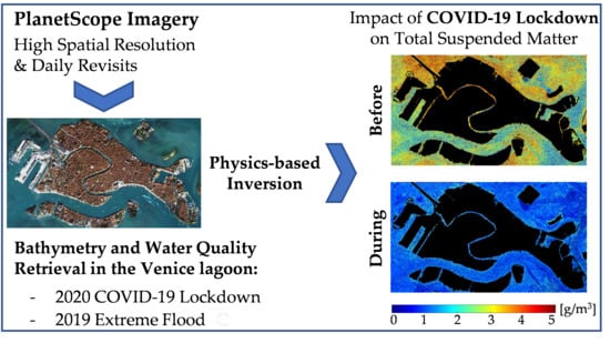
Physics-based Bathymetry and Water Quality Retrieval Using PlanetScope Imagery: Impacts of 2020 COVID-19 Lockdown and 2019 Extreme Flood in the Venice Lagoon

Abstract

The recent PlanetScope constellation (130+ satellites currently in orbit) has shifted the high spatial resolution imaging into a new era by capturing the Earth’s landmass including inland waters on a daily basis. However, studies on the aquatic-oriented applications of PlanetScope imagery are very sparse, and extensive research is still required to unlock the potentials of this new source of data. As a first fully physics-based investigation, we aim to assess the feasibility of retrieving bathymetric and water quality information from the PlanetScope imagery. The analyses are performed based on Water Color Simulator (WASI) processor in the context of a multitemporal analysis. The WASI-based radiative transfer inversion is adapted to process the PlanetScope imagery dealing with the low spectral resolution and atmospheric artifacts. The bathymetry and total suspended matter (TSM) are mapped in the relatively complex environment of Venice lagoon during two benchmark events: The coronavirus disease 2019 (COVID-19) lockdown and an extreme flood occurred in November 2019. The retrievals of TSM imply a remarkable reduction of the turbidity during the lockdown, due to the COVID-19 pandemic and capture the high values of TSM during the flood condition. The results suggest that sizable atmospheric and sun-glint artifacts should be mitigated through the physics-based inversion using the surface reflectance products of PlanetScope imagery. The physics-based inversion demonstrated high potentials in retrieving both bathymetry and TSM using the PlanetScope imagery.

1. Introduction

The PlanetScope constellation has bridged the long-lasting gap between the high spatial and the high temporal resolution of spaceborne imagers by means of more than 130 CubeSats (known also as Doves) currently in orbit [1,2]. The PlanetScope operated by Planet Labs, Inc. is the largest Earth-observing constellation of small satellites in the size of 10×10×30 cm³ carrying sensors with four or five bands [2]. This high number of CubeSat imagers allows for daily acquisitions over the entire land surface of the Earth and near-shore coastal environments at the spatial resolution of about 3 m. The availability of PlanetScope imagery opens up new opportunities for a wide range of Earth observation applications by providing insights into the changes of land-cover/use and biophysical attributes with spatiotemporal details never previously possible. In this context, PlanetScope constellation potentially offers a unique means of monitoring the dynamics of aquatic biophysical parameters, such as in-water constituents even for small bodies of inland water. The high revisit frequency, i.e., daily overpasses, significantly enhances the capability of capturing cloud-free imagery, which is a remarkable step toward near real-time monitoring of the inland/coastal waters [1,3,4].

The application of PlanetScope imagery into aquatic systems has yet been limited to very few studies [1,5,6]. This can be initially related to the fact that this constellation is new and its imaging capacity has been maximized only recently by about 130 satellites in orbit (early 2020 [2]). On the other hand, the variable radiometric quality, inconsistent radiometric calibration across multiple platforms, and relatively low spectral resolution are central challenges for aquatic applications [1,7,8]. The existing attempts to demonstrate potentials of the PlanetScope imagery in the area of aquatic remote sensing are mostly based upon empirical approaches. The empirical methods employ in-situ samples of the parameter of interest (e.g., bathymetry, turbidity, etc.) to infer a relation between image-derived features (e.g., single bands, band ratios, etc.) and the given parameter through a supervised regression analysis [9,10,11,12,13]. These methods are mainly employed for retrieval of individual biophysical parameters such as bathymetry [14,15,16] and in-water constituents like chlorophyll-a (Chl-a), total suspended matter (TSM), and colored dissolved organic matter (CDOM) [17,18]. In the context of exploiting PlanetScope imagery, the bathymetry of a coastal area in Greece is mapped using these images, by calibrating a regression model using in-situ measurements of water depths [1]. In a similar work, the bathymetry of a coastal area in Egypt is derived from PlanetScope imagery based on Lyzenga’s linear regression model [19] using blue and green bands [5]. A semi-empirical algorithm is employed to retrieve the turbidity in the San Francisco Bay (USA) and the coastal areas in the UK [20]. The PlanetScope imagery demonstrated potentials also in the classification of seagrass species in the Karimunjawa Islands (Indonesia), based on unmixing and object-based techniques without applying a water-column correction [6]. A high resolution (2 m) imagery from Pléiades satellite, with four bands similar to the PlanetScope data, are also used for estimation of turbidity through an empirical approach in an estuary environment [21]. Although the empirical (regression-based) methods are straightforward to apply, they require field data collection simultaneous with the image acquisition which limits their applications.

In this study, we aim at retrieving bathymetry and concentration of TSM using PlanetScope imagery based on a fully physics-based approach. The remote mapping of bathymetry using satellite data is of particular importance in a wide range of aquatic science and management applications. This is because traditional methods of bathymetric surveys, such as single/multi-beam echo sounders (SBES/MBES) or airborne lidar bathymetry are expensive and limited in both time and space. Bathymetry impacts the primary production in the aquatic systems as the absorption by pure water exponentially limits the penetration of the light into the water column. Furthermore, information on bathymetry is critical for navigation purposes and the spatial variations of the water depth can be considered as an indicator of bed topography [1]. TSM refers to organic and mineral solids suspended in the water column, which is closely linked with water transparency/turbidity and Secchi disk depth [22]. The monitoring of TSM can contribute to the assessment of water quality and studies on sediment transportation [22,23]. We examine the feasibility of a physics-based inversion of the PlanetScope radiometric data for retrieving bathymetry and TSM in a challenging shallow water environment. Unlike empirical methods, the physics-based methods rely on the radiative transfer modeling [24,25,26]. In this context, the physics-based inversion accounts for the absorption and backscattering properties of different media that light interacts with through its traveling path, i.e., atmosphere, water surface, and column as well as the bottom substrate in optically-shallow waters. The total-at-sensor signal is composed of several radiance components upwelling after interacting with these media. Considering the mixed radiance, observed by the sensor, only the component of radiance is the desired signal that contains the information about the parameter of interest. For instance, only bottom-reflected radiance contains bathymetric information. Therefore, water depth can be retrieved only in optically-shallow waters where the light can penetrate the entire water-column and travel back to the sensor after having an interaction with the substrate [27,28,29]. Other radiance components, such as the contributions of water column and surface can complicate depth retrieval particularly if they are spatially variable over the water body. Likewise, the bottom-reflected radiance and its variability can induce challenges into the estimation of in-water constituents. In general, the characteristic spectral feature of a given biophysical parameter is subject to degradation or interference in the presence of other radiance components, particularly if the desired component is not dominant [17,30,31,32]. The atmospheric effects also can contaminate the water-leaving signal to a large extent as water bodies may reflect only up to 10 % of the downwelling irradiance, due to the high attenuation of the light in pure water [10,17]. Therefore, the signal to noise ratio (SNR) is a critical factor in the aquatic applications of remote sensing. In this context, empirical techniques by incorporating relatively robust spectral features like band ratios and/or multiple features can mitigate the confounding atmospheric effects [9,15]. However, the absolute radiances at different wavelengths are not as important as they are for physics-based inversion. This is evident from some studies using top-of-atmosphere (TOA) data through the regression analysis for retrieving bathymetry or in-water constituents [10]. In contrast, the absolute radiances are of particular importance in physics-based inversion, which calls for an appropriate modeling of the atmospheric artifacts [26,33,34]. Moreover, the physics-based methods require knowledge about the inherent optical properties (IOPs) of the water-column and substrate types/compositions in optically-shallow waters. The physics-based methods such as Water Color Simulator (WASI) processor [25,35] allow for simultaneous retrieval of the variable parameters involved in the inversion such as bathymetry and in-water constituents.

We pursue the following objectives: the first one is to assess the feasibility of performing a physics-based inversion in an optically-shallow environment using the surface reflectance products of PlanetScope imagery. We aim to adapt the WASI processor for retrieving the bathymetry and TSM from PlanetScope imagery. WASI varies a set of parameters in a number of iterations to reduce the mismatch between an observed/image spectrum and radiative transfer simulations. The PlanetScope imagery provides a limited number of spectral bands, i.e., four or five bands spanning over visible and near-infrared (NIR) portion of the spectrum. In this context, the total number of variable (fitting) parameters through WASI inversion becomes relatively high compared to the number of spectral bands. This poses a challenge for processing the PlanetScope imagery by introducing spectral and mathematical ambiguities. The second objective is to demonstrate the application of multitemporal PlanetScope imagery in the context of bathymetry retrieval and assessing the impact of the coronavirus disease 2019 (COVID-19) lockdown as well as an extreme flooding (November 2019) on the turbidity of the Venice lagoon. The boat traffic that normally crowds the channels almost vanished due to the COVID-19 lockdown restrictions applied by the Italian government leading to water transparency indicated in several field reports [36,37]. The reduction of the water turbidity during the lockdown is mainly attributed to the settlement of the sediment at the bottom in the absence of water perturbations and waves shaped by the boat movements. We have also analyzed an opposite event when there was extreme flooding (November 2019) in Venice leading to a high level of turbidity. These two extreme events serve as benchmarks for evaluating the potentials of the newly available PlanetScope imagery regarding our research objectives.

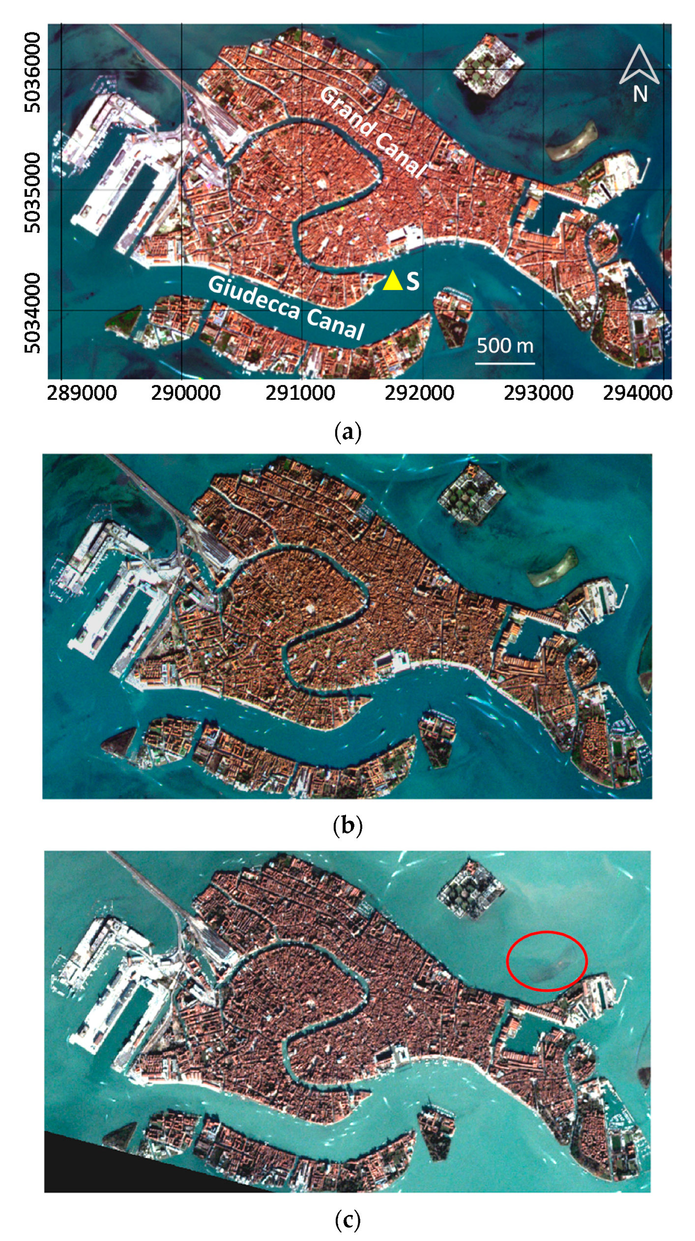
2. Study Area and Dataset

The Venice lagoon is a shallow basin located in northeast Italy and connected to the Adriatic Sea. The study area is selected within the lagoon, which contains the Venice city and surrounding water. The closest connection to the sea is the Lido inlet in the studied region. The hydrodynamics of the lagoon is affected by several factors, such as meteorological conditions (e.g., wind waves), fluvial inflows, and variations in tidal levels [38]. To assess the performance of WASI on the PlanetScope data, two extreme events are considered: (i) the COVID-19 lockdown in spring 2020, and (ii) a sequence of floods occurred in mid-November 2019 - unprecedented since 1969 - which were driven by a combination of extreme high tides, severe storms, and inland water inflows [39]. For the former event, we have analyzed three images acquired before (23 January, 15 and 28 February 2020) and three images captured during (19 March, 8 and 13 April 2020) the COVID-19 pandemic lockdown (Figure 1a,b). The significant reduction of the number of active ships due to the COVID-19 lockdown is evident in the main channels by visually comparing Figure 1a (about 9 ships) and Figure 1b (about 67 ships). For the latter case, we considered an image acquired in a cloud-free condition during the flood period (26 November 2019) to examine the physics-based inversion of PlanetScope imagery in a turbid-water condition (Figure 1c).

The PlanetScope images are acquired at 3.7 m pixel size (nadir viewing) and resampled to 3 m. The spectral resolution is limited to four bands (RGB-NIR) though newly launched CubeSats imagers also include an extra red-edge band (transition between red and NIR, around 700 nm). In our analyses, we considered 4-band imagery (455−515 nm, 500−590 nm, 590−670 nm, 780−860 nm) with a dynamic range of 12-bit. We process the surface reflectance images which are available as PlanetScope ortho scene products (level−3B). The atmospheric correction of this product is performed by the data provider based on 6S radiative transfer model by employing ancillary data derived from Moderate Resolution Imaging Spectroradiometer (MODIS) products (e.g., water vapor, ozone, and aerosol data) [2]. The level−3B imagery is orthorectified and geometrically corrected [2]. We also use in-situ data from a tide gauge in the study region for the relative assessment of the multitemporal bathymetry maps derived in different tidal levels. The tide levels are recorded at Punta della Salute (shown in Figure 1a).

3. Method

The core of our physics-based method is based on inverting a model that approximates the complex interaction between light and (i) the atmosphere, (ii) the air/water interface, (iii) the water column and (iv) the bottom substrates. The reflection, scattering, and absorption properties of these media are used to describe the contribution of these components on the total radiance observed by a satellite sensor. There are different methods for the physics-based estimation of bathymetry and in-water constituents [34,40]. Some of the methods, such as Case-2 Regional/Coast Colour (C2RCC) [41], are designed for processing optically-deep waters and specific for some pre-defined satellite sensors. Our analyses are based upon WASI, which is a publicly available processor [42], allowing for both forward and inverse radiative transfer modeling in optically deep and shallow waters, independent from the sensor [25,43]. The main equations used in WASI are briefly summarized in the following; for more details see the WASI manual [42,44].

3.1. Adaptation of WASI for Processing PlanetScope Imagery

Since atmospherically corrected PlanetScope data are given in units of reflectance, all calculations in WASI are also made in terms of reflectance. The measured reflectance $R_{rs}\left(\lambda \right)$ is the sum of a component from the water, called remote sensing reflectance [24,45] and a component caused by reflections at the water surface,

$$R_{rs}\left(\lambda \right)=\frac{\zeta ·r_{rs}\left(\lambda \right)}{1-\Gamma ·r_{rs}\left(\lambda \right)}+R_{rs}^{surf}\left(\lambda \right).$$

(1)

where $r_{rs}$ is the ratio of upwelling radiance to downwelling irradiance just below the water surface. $\zeta \approx$ 0.52 is the water-to-air radiance divergence factor; the denominator with $\Gamma \approx$ 1.6 accounts for reflection of upwelling radiance in the water at the water surface. The models of Albert [46,47] are used for simulating $r_{rs}\left(\lambda \right)$. It expresses $r_{rs}$ of optically deep water as follows,

$$\begin{gathered} r_{rs}^{deep}\left(\lambda \right)= \\ 0.0512·u\left(\lambda \right)·(1+4.6659·u\left(\lambda \right)-7.8387·u{\left(\lambda \right)}^2+5.4571·u{\left(\lambda \right)}^3) \\ \left(1+\frac{0.1098}{cos{\theta }_{sun}^{\prime }}\right)·\left(1+\frac{0.4021}{cos{\theta }_v^{\prime }}\right)·\left(1-0.0044v_w\right). \end{gathered}$$

(2)

where ${\theta }_{sun}^{\prime }$ is the solar zenith angle in water, ${\theta }_v^{\prime }$ the viewing zenith angle in water and $v_w$ the wind speed in units of [m s⁻¹]. As observation was close to nadir and wind speed has only a very small effect on $r_{rs}$, ${\theta }_v^{\prime }$ = 0 and $v_w$ = 0 are set. The wavelength-dependent function $u\left(\lambda \right)$ is given by:

$$u\left(\lambda \right)=\frac{b_b\left(\lambda \right)}{a\left(\lambda \right)+b_b\left(\lambda \right)}.$$

(3)

$\mathrm{where} a\left(\lambda \right)$ is the absorption coefficient of the water layer and $b_b\left(\lambda \right)$ its backscattering coefficient. Both are expressed as the sum of the individual optically active components:

$$a\left(\lambda \right)=a_w\left(\lambda \right)+a_{CDOM}\left({\lambda }_0\right)·exp\left\{-S·\left(\lambda -{\lambda }_0\right)\right\}+C_{phy}·a_{phy}^{*}\left(\lambda \right)+C_{NAP}·a_{NAP}^{*}\left({\lambda }_0\right)·\exp \left\{-S_{NAP}·\left(\lambda -{\lambda }_0\right)\right\},$$

(4)

$$b_b\left(\lambda \right)=b_{b,w}\left(\lambda \right)+C_{phy}·b_{b,phy}^{*}\left(\lambda \right)+C_{NAP}·b_{b,NAP}^{*}\left(\lambda \right).$$

(5)

$a_w\left(\lambda \right)$ and $b_{b,w}\left(\lambda \right)$ are the absorption [48,49] and backscattering [50] coefficients of pure water, respectively. Three types of water constituents are considered: Colored dissolved organic matter (CDOM), phytoplankton (phy), and non-algal particles (NAP). The absorption coefficient of CDOM at the wavelength ${\lambda }_0$ = 440 nm, $a_{CDOM}\left(440\right)$, and NAP concentration, $C_{NAP}$, are treated as unknowns during inverse modelling, whereas phytoplankton concentration $C_{phy}$ is kept constant since a pre-fit analysis of the used images has shown that changing $C_{phy}$ has minimal impacts on the retrieval of the target parameters bathymetry and TSM. The spectral slopes of CDOM and NAP absorption are set to standard values of $S$ = 0.014 nm⁻¹ [51,52] and $S_{NAP}$ = 0.011 nm⁻¹ [53]. Since diatoms are frequently the main phytoplankton species in the study area [54], the diatoms spectrum from the WASI database is used for the specific absorption coefficient of phytoplankton, $a_{phy}^{*}\left(\lambda \right)$. The specific absorption coefficient of NAP at ${\lambda }_0$ = 440 nm is set to $a_{NAP}^{*}\left(440\right)=$ 0.027 m² g⁻¹ [55], and the specific backscattering coefficient of NAP is treated as a wavelength-independent function with $b_{b,NAP}^{*}\left(\lambda \right)$ = 0.0086 m² g⁻¹ [56]. The concentration of total suspended matter is the sum of $C_{phy}$ and $C_{NAP}$:

$$C_{TSM}=C_{phy}+C_{NAP}\approx C_{NAP}.$$

(6)

$C_{NAP}$ is three orders of magnitude higher than $C_{phy}$ in the Venice lagoon (1–3 g m⁻³ vs. ~2 mg m⁻³), hence $C_{TSM}$ and $C_{NAP}$ are approximately equal.

For optically-shallow water $r_{rs}$ is calculated as follows [46,47]:

$$\begin{gathered} r_{rs}^{shallow}\left(\lambda \right)=r_{rs}^{deep}\left(\lambda \right)·\left[1-1.1576·exp\left\{-\left(K_d\left(\lambda \right)+k_{uW}\left(\lambda \right)\right)·z_B\right\}\right]+ \\ \frac{1.0389}{\pi }·f_B·a_B\left(\lambda \right)·exp\left\{-\left(K_d\left(\lambda \right)+k_{uB}\left(\lambda \right)\right)·z_B\right\}. \end{gathered}$$

(7)

The first term on the right-hand side is the reflectance of a water layer of thickness $z_B$, the second term is the contribution of the bottom. $K_d$ is the diffuse attenuation coefficient of downwelling irradiance, $k_{uW}$ the attenuation coefficient for upwelling radiance originating from the water layer, $k_{uB}$ the attenuation coefficient for upwelling radiance from the bottom, $z_B$ water depth, $a_B\left(\lambda \right)$ the albedo (irradiance reflectance) of the bottom substrate, and $f_B$ the brightness of the actual bottom substratum relative to the reference spectrum $a_B\left(\lambda \right)$. The attenuation coefficients are a function of $a\left(\lambda \right)$ and $b_b\left(\lambda \right)$; for details see [46,47].

The reflections at the water surface are simulated using the three-component model of Gege [35] for the sky radiance that is reflected in the viewing direction:

$$L_{sky}\left(\lambda \right)=g_{dd}{E}_{dd}\left(\lambda \right)+g_{dsr}{E}_{dsr}\left(\lambda \right)+g_{dsa}{E}_{dsa}\left(\lambda \right).$$

(8)

The three terms in Equation (8) describe sun glint and reflection by the blue and gray components of sky light caused by molecules and aerosols: $E_{dd}\left(\lambda \right)$ is the direct downwelling irradiance from the sun disk, $E_{dsr}\left(\lambda \right)$ is the diffuse downwelling irradiance caused by Rayleigh scattering, and $E_{dsa}\left(\lambda \right)$ is the diffuse downwelling irradiance caused by aerosol scattering. The parameterization of $E_{dd}\left(\lambda \right)$, $E_{dsr}\left(\lambda \right)$ and $E_{dsa}\left(\lambda \right)$ in terms of aerosols, water vapor, and ozone is described in [57], which is adapted from the model of Gregg and Carder [58].

The weights $g_{dd}$, $g_{dsr}$ and $g_{dsa}$ represent the intensity of each irradiance component that is reflected in sensor direction. They can differ from pixel to pixel if waves undulate the water surface. The fraction of sky radiance due to direct solar radiation, $g_{dd}$, is typically in the order of 0–0.03 sr⁻¹ outside the obvious sun-glint region of an image. A hypothetic isotropic sky is defined by fractions of sky radiance due to molecule and aerosol scattering of $g_{dsr}$ = $g_{dsa}$ = 1/$\pi$. The surface reflectance is given by,

$$R_{rs}^{surf}\left(\lambda \right)={\rho }_L\left({\theta }_v\right)\times \frac{L_{sky}\left(\lambda \right)}{E_{dd}\left(\lambda \right)+E_{dsr}\left(\lambda \right)+E_{dsa}\left(\lambda \right)}$$

(9)

where ${\rho }_L\left({\theta }_v\right)$ is the Fresnel reflection for a viewing angle of ${\theta }_v$ [59]; ${\rho }_L\left(0\right)$= 0.020 for nadir observation. This model is able to correct accurately surface reflections by treating $g_{dd}$, $g_{dsr}$ and $g_{dsa}$ as fit parameters [35,60].

As mentioned, WASI can perform both forward and inverse radiative transfer modeling. The inverse modeling of multi- and hyper-spectral images employed in this study is implemented in a module called WASI-2D [35]. Its flexibility in parametrization allows adaptation to a wide range of in-water optical conditions and processing of data from any passive optical sensor with bands in the spectral range from 380 to 1000 nm [35,61]. Inverse modeling is accomplished by simulating $R_{rs}\left(\lambda \right)$ using Equation (1) for different values of the unknown model parameters, called fit parameters. The goal of the repeated simulations is to find the best match with the observed image spectrum. A cost function assesses the correspondence between measured spectrum $R_{rs}^{measured}\left(\lambda \right)$ and simulated spectrum $R_{rs}^{simulated}\left(\lambda \right)$. Different cost functions are implemented in WASI. The Mean Absolute Percentage Difference (MAPD) provided the most consistent results across the image pixels:

$$\Delta =\frac{1}{N}{\displaystyle \sum }_{i=1}^N\left|1-\frac{R_{rs}^{simulated}\left({\lambda }_i\right)}{R_{rs}^{measured}\left({\lambda }_i\right)}\right|.$$

(10)

where ${\lambda }_i$ denotes the center wavelength of band number i. In the case of PlanetScope $i$ runs from 1 to $N$ = 4. The inversion algorithm makes use of the Downhill Simplex algorithm [62,63] to find the set of fit parameters, which minimizes the residual $\Delta$.

Data analysis by inverse modeling requires the initialization of various parameters defining the in-water and (in case of optically-shallow water) bottom optical conditions. Then, the inversion performs a series of iterations in order to converge to the values of parameters that show the best match between the simulated and image spectra. The fit parameters can be retrieved throughout the image by performing this procedure for every pixel individually. Although various parameters can be assigned as fit parameters, it is critical to maintain their number as limited as possible. This is necessary to minimize errors. introduced by spectral ambiguities, i.e., to reduce the number of parameters inducing similar spectral characteristics. Mathematically unambiguous solutions of the inversion problem require that the number of fit parameters is smaller or equal to the number of bands. Using more fit parameters than bands requires careful initialization and constraining the fit ranges, but can nevertheless introduce noise to the derived parameters which is associated with the remaining spectral ambiguities. The useful number of fit parameters is therefore small for processing images with low spectral resolution such as those of the PlanetScope constellation. The initialization of the fit parameters and their ranges can be done by fitting some representative image pixels repeatedly with varying fit settings or using pre-knowledge available about the study area. The choice of the fit parameters and adaptation of the WASI inversion to the challenging data processing of our case study are explained in the next subsection.

3.2. Parametrization of WASI

Although the region of interest is always the same, two different inversion schemes are used: (i) a shallow-water inversion for the COVID-lockdown case study, which includes the estimation of bathymetry, and (ii) a deep-water inversion for the flood period case study (see Section 2 for the case studies). In the latter case, we decided to use the deep-water model (Equation (2)) based on visual inspection and pre-fit analyses. The high water-level and the increased turbidity during the flood period significantly limited the penetration of the light so that the bottom-reflected radiance was hardly detectable.

3.2.1. Shallow-Water Inversion

The images acquired before and during the COVID-19 lockdown are processed by applying the shallow-water model (Equation (7)). As mentioned before, it is important to minimize the number of fit parameters as much as possible to avoid overfitting which may introduce unnecessary spectral ambiguities due to the low spectral resolution of the PlanetScope imagery. As mentioned in Section 3.1, $C_{phy}$ is treated as constant with a value of 2 mg/m³, and diatoms are considered as the main species of the phytoplankton community [54]. We also assume a sandy bottom for the selection of the bottom substrate [64]. The specific absorption coefficient of diatoms, $a_{phy}^{*}\left(\lambda \right)$, and the albedo of sand, $a_B\left(\lambda \right)$, are taken from the WASI database. We perform the shallow water inversion with five fit parameters listed in

Table 1. Fit parameters of WASI and associated initial values for the shallow-water inversion.

Fit Parameter	Initial Value	Min	Max	Units	Description
$a_{CDOM}\left(440\right)$	0.1	0	50	m−1	Absorption coefficient of CDOM at 440 nm
$C_{NAP}$	0.8	0.1	100	g m−3	Concentration of NAP
$z_B$	2	0	1000	m	Bottom depth (water depth)
$f_B$	2	0	10		Relative brightness of sand
$g_{dd}$	0.67	−1	10	sr−1	Fraction of sky radiance due to direct solar radiation

. $z_B$ is the water depth and $f_B$ represents the brightness of the actual bottom substrate relative to the sand reference spectrum. $C_{NAP}$ stands for the concentration of TSM (see Equation (6)) and $a_{CDOM}\left(440\right)$ is the absorption coefficient of CDOM at 440 nm. $g_{dd}$ is the sun glint intensity. As the spectral shape of sun glint is similar to the straylight in the atmosphere, $g_{dd}$ can also model to some extent errors of atmospheric correction, caused by under- or over-estimation of the path radiance. Negative $g_{dd}$ values correct for overestimated path radiances. The pre-fits revealed unusually high $g_{dd}$ values, which indicates major atmospheric artifacts in the PlanetScope images that needed to be considered through the inversion.

3.2.2. Deep-Water Inversion

We apply the deep-water model (Equation (2)) for processing the image acquired during the flood condition (26 November 2019). As the estimation of bathymetry is not feasible based on deep-water inversion, the water depth $z_B$ and the bottom parameter $f_B$ are removed from the fit parameters. However, the pre-fits suggested using two additional parameters for compensation of the atmospheric effects. These parameters are the fractions of sky radiance due to Rayleigh and aerosol scattering, $g_{dsr}$ and $g_{dsa}$. Stable inversion results are obtained by setting the initial value of $C_{NAP}$ to a high value (6 g/m³) which was expected due to the increased turbidity of the water during flood conditions. Therefore, the inversion is performed by considering five variable parameters (

Table 2. Fit parameters of WASI for the deep-water inversion.

Fit Parameter	Initial Value	Min	Max	Units	Description
$a_{CDOM}\left(440\right)$	0.1	0	50	m−1	Absorption coefficient of CDOM at 440 nm
$C_{NAP}$	6	0.1	100	g m−3	Concentration of NAP
$g_{dd}$	0.67	−1	10	sr−1	Fraction of sky radiance due to direct solar radiation
$g_{dsr}$	0.318	0	10	sr−1	Fraction of sky radiance due to Rayleigh scattering
$g_{dsa}$	0.318	0	10	sr−1	Fraction of sky radiance due to aerosol scattering

).

4. Results and Discussion

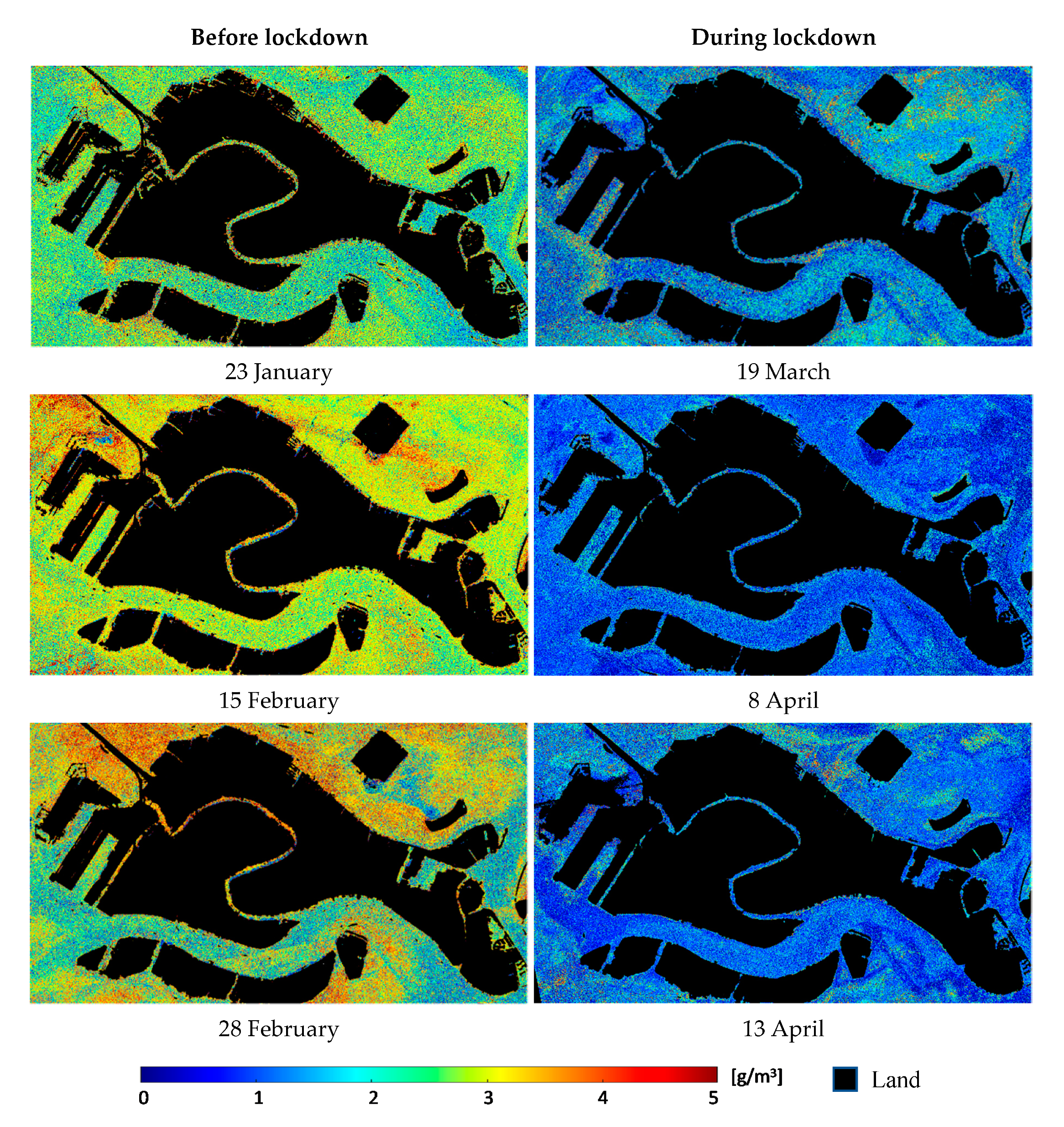
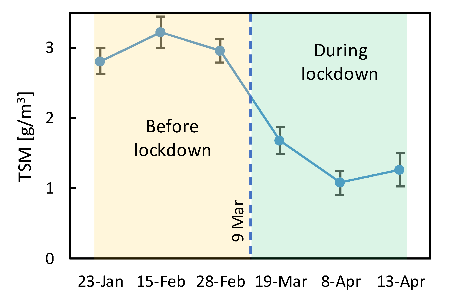
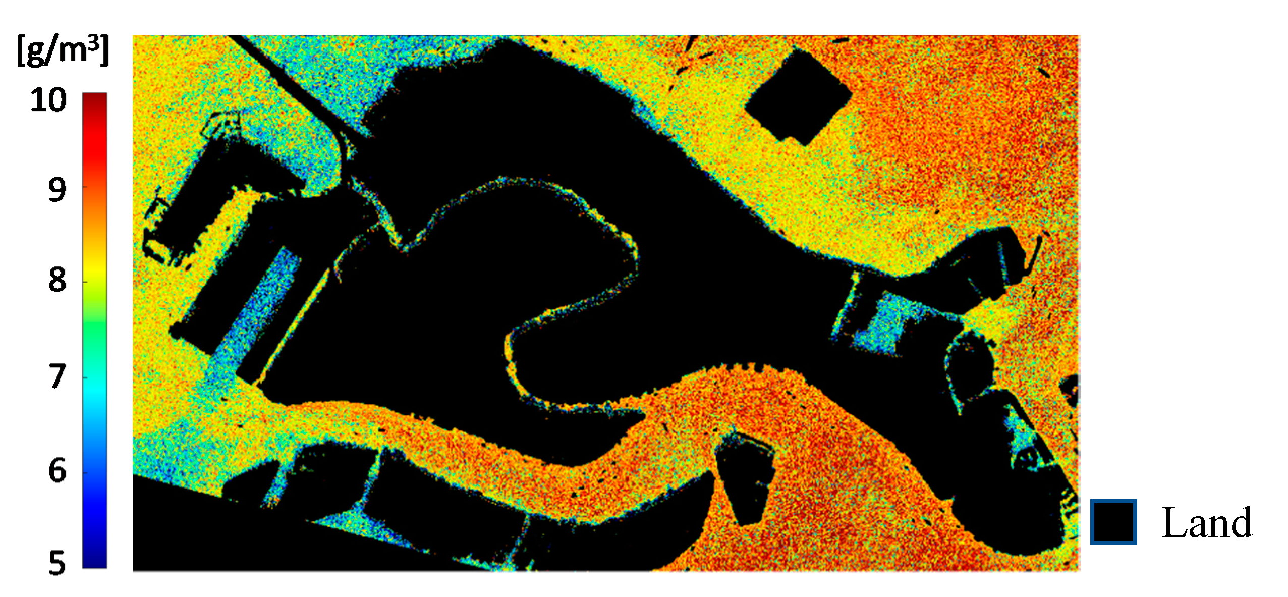
4.1. Retrievals of TSM

The TSM maps derived from the shallow-water inversion are presented in Figure 2 for the periods before and during the COVID-19 lockdown.

As evident, the concentration of TSM remarkably decreased during the lockdown period. This is in accordance with several site observations reported in the news about the outstanding reduction of the turbidity [36,37]. TSM is strongly correlated to the turbidity/transparency of the water [23]. The abrupt change of TSM identified from analyzing the images before and during this benchmark event reveals the effectiveness of the physics-based approach in retrieving this constituent from PlanetScope imagery.

The time series of average TSM estimates along with the associated standard deviations are shown in Figure 3. The trend indicates a relatively stable concentration of TSM before the lockdown with an average value near 3 g/m³. The concentration of TSM decreases notably during the lockdown so that the average value reaches to about 1.4 g/m³, corresponding to ~ 50 % reduction, compared to the period before lockdown. During the country-wide lockdown due to the COVID-19 pandemic in Italy (starting from 9 March 2020), the channels and waterways of Venice lagoon appeared nearly empty [65]. Therefore, the reduction of the TSM concentration highlights the major impact of the boat traffic in the suspension of the sediments in the water column before the lockdown. Other studies also confirm the major impacts of the boat traffic in the sediment suspension in the Venice lagoon [66].

The TSM map derived from the deep-water inversion of the image acquired during the extreme flooding in the Venice lagoon is shown in Figure 4. The average TSM is 7.8 g/m³ and the standard deviation of 0.75 g/m³. The concentration of TSM during the severe flooding condition is hence more than doubled compared to normal conditions (3 g/m³). This experiment indicates the utility of PlanetScope imagery in mapping the TSM concentration of turbid waters, based on physics-based inversion. This can contribute to the near real-time monitoring of the TSM particularly in small water bodies given the high spatiotemporal resolution of the constellation that enables capturing the high spatiotemporal variability of suspended solids.

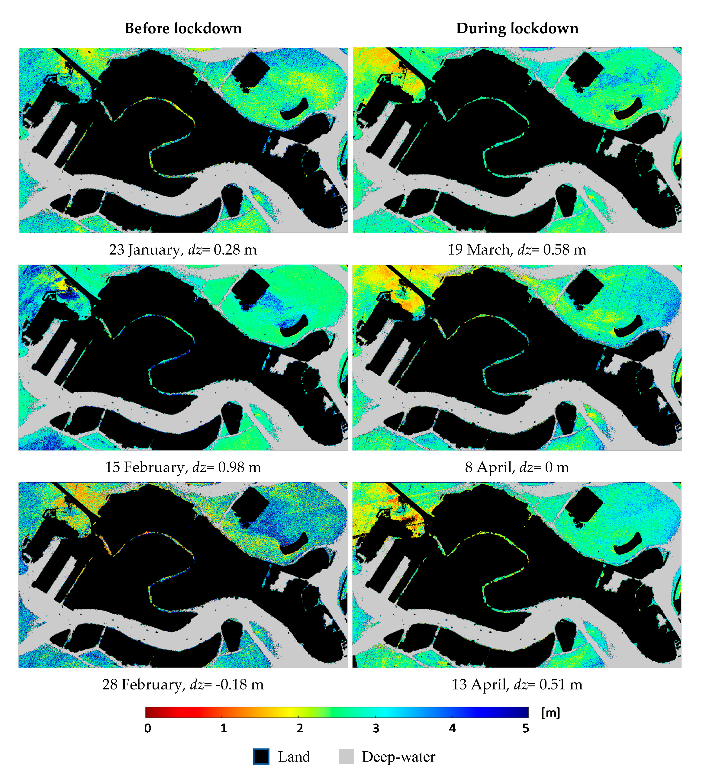
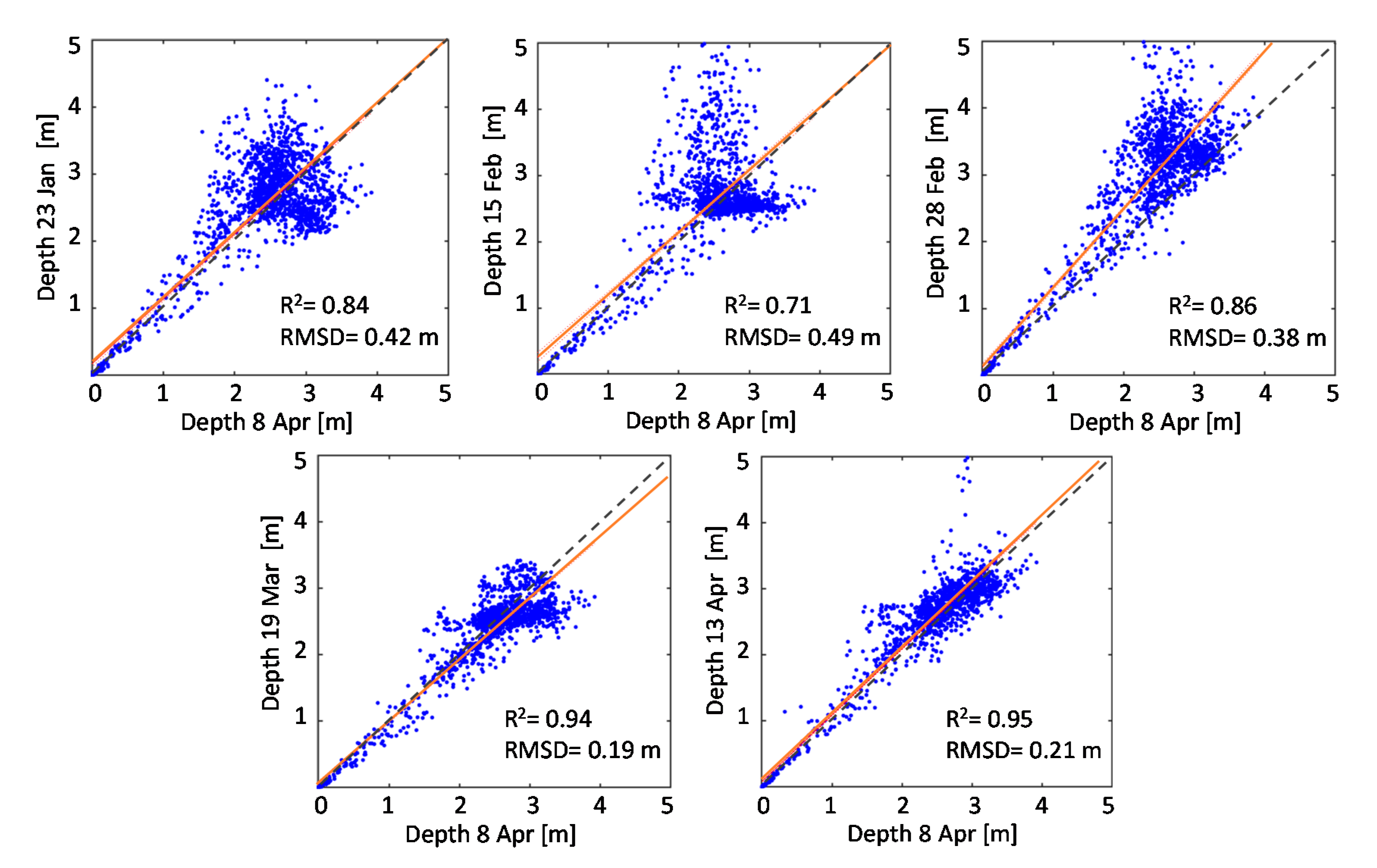
4.2. Retrievals of Bathymetry

We examine the potential of PlanetScope imagery in the estimation of bathymetry through the physics-based shallow-water inversion assuming that bathymetry remained relatively stable during the period of observation excluding the tidal effects. It can be expected that the high variability of the environmental conditions, in particular the strongly changed turbidity, leads to inconsistent results of the derived water depths in all cases, in which the algorithm cannot determine bathymetry reliably from the data. The potential of the PlanetScope data for deriving water depth, and also the useable depth range, can thus be assessed by comparing the derived water depths.

The tidal variations change the water level in the studied area. To make the derived bathymetry maps comparable and to better visualize the depth differences, we use the bathymetry map from 8 April 2020 as reference. The reference map is chosen among those during the lockdown as it is expected that the clear water condition yields more accurate depth retrievals. Then, a depth offset (dz) is applied to every other bathymetry map to harmonize the bathymetric maps by mitigating the tidal effects (Figure 5). The offset-correction is performed based on image-derived values of depth. In this context, the average difference of depths (excluding the deep-water pixels), with respect to the reference map is considered as the offset (dz) for every bathymetry map. Note, that the offset-correction can be done also based on the tide gauge data. However, this might introduce uncertainties as a single point measurement is less representative for the entire area and the station measurements involve some errors as well. The computed offsets are in a good agreement with those derived from the tide gauge station (R²= 0.94).

We masked the parts of the study area with depths above 5 m (gray-shaded area in Figure 5, mainly Giudecca Canal with average depth about 12 m [67,68]) as the inversion showed large biases with respect to multibeam echo sounder data available from the deep channels of the studied area [67,68]. The deeper the water, the weaker is the bottom-reflected signal due to the strong absorption by the water column. The band designation along with factors such as the radiometric resolution and in-water optical conditions define the maximum detectable depth [69]. Here, the turbidity of the water, the limited number of bands provided by the PlanetScope imagery and the uncertainties from atmospheric correction (large offsets had to be corrected) pose a challenge to bathymetry estimation for depths above approximately 5 m. The retrieved water depths for the shallow areas (< 5 m) are in visually good agreement with the bathymetric maps reported in previous studies [70,71].

The patterns and absolute values of water depth show good agreements among all the offset-corrected bathymetry maps (Figure 5). We assessed the consistency of the offset-corrected bathymetry maps by performing regression analyses between the depth values of each map with those of the reference map (8 April 2020). In this context, we resampled the depth maps to a coarser resolution by averaging the depth values of 10 × 10 pixels for the non-masked pixels. If there were less than 5 water pixels in a 10 × 10 window, the resampled pixel was masked. This averaging mitigates the effect of possible co-registration misalignments and also removes the noise. Figure 6 illustrates the regression analyses (N = 1907). The number of water pixels is much lower than in Figure 5 because the averaging reduced the image size by a factor of 100. The statistics including the coefficient of determination (R²) and root mean square difference (RMSD) are shown in each plot. The depth estimates are in good agreement with an average R² of 0.86 and an average RMSD of 0.33 m. These analyses confirm the consistency of the depth estimates at changing TSM concentration, which in turn indicates the potential of the PlanetScope imagery for bathymetric estimation through physics-based modeling. The depth range of very good agreements is larger for the period during the lockdown. This can be attributed to the improved visibility of the bottom in the less turbid conditions.

It should be noted that small systematic errors in the bathymetry maps can be expected due to uncertainties of assuming a constant offset for all the pixels. This is because the tidal effects can vary spatially that can introduce a regionally variable depth offset across the study area. Furthermore, the bed topography in the Venice lagoon is subject to major changes over time due to tidal effects and human-induced activities [72]. For instance, the morphodynamics of a shallow tidal system such as the Venice lagoon is highly influenced by sediment transportation in the presence of ship and boat traffic [38,64,71]. Therefore, the temporal changes in the bottom topography (erosion and deposition processes) can also affect the distribution/pattern of bathymetry. All these effects can introduce noise to Figure 6. However, the main noise sources are the uncertainties of the retrieval algorithm introduced by the described limitations of the PlanetScope data and the environmental conditions.

5. Conclusions and Outlook

The high spatial resolution in combination with daily revisits of the PlanetScope constellation potentially enables advances in near real-time monitoring of inland/coastal aquatic systems. The meter-scale data offered by this constellation is of particular importance in studying small water bodies (e.g., narrow fluvial systems) where the spatial resolution of operational multispectral satellites such as Sentinel-2 and Landsat-8 (10−30 m) is not sufficient. The daily acquisition enhances the chance of acquiring cloud-free images allowing for better capturing the dynamics of in-water biophysical parameters, as well assessment of the changes after rapid events, such as floods. Up until now, studies on the application of PlanetScope imagery to aquatic science and management are very sparse. This study demonstrates the suitability of this new source of imagery for physics-based inversion methods at the example of bathymetry and suspended matter concentration determination.

The limited number of spectral bands provided by the PlanetScope imagery poses a major challenge to the physics-based inversion of bio-optical parameters by introducing mathematical and spectral ambiguities through the fitting process. Therefore, the fit parameters of the physics-based model need to be restricted to the dominant environmental variables of the area of interest. This is to maintain the number of fit parameters as limited as possible to ensure reliable estimates. Using pre-knowledge about the bio-optical conditions in the study area can assist in regional model adaptation and reducing the number of unknows. For instance, we used the optical properties of diatoms and fixed phytoplankton concentration at 2 mg m⁻³ according to a priori knowledge of the test site. However, the restriction of the fit parameters can be challenging, especially when various environmental parameters are variable like in shallow waters. The limited number of bands also restricts the accuracy and range of parameters (e.g., maximum depth), extracted from the PlanetScope imagery. This is because channels with low spectral resolution and centered at wavelengths not optimized for a certain application provide less sensitivity to the ’spectral fingerprint’ of a given bio-optical parameter than a specialized sensor would.

The shallow-water inversion may benefit in some parts of our studied area from introducing macrophytes as an extra bottom type. However, this increase in the number of fit parameters may reduce the reliability of retrievals. Since the parameter used for modeling sun glint and artifacts from atmospheric correction was unusually high, we conclude that the atmospheric path radiance had been underestimated during preprocessing by PlanetScope. Therefore, the atmospheric correction methods should be further examined on the PlanetScope imagery to meet the needs for high-quality radiometric data for aquatic applications.

As a first attempt to apply a fully physics-based approach, we obtained promising results from processing PlanetScope imagery by demonstrating their potential in mapping bathymetry and capturing the variations of TSM concentration during the selected extreme benchmark events. However, further studies are required to broaden the assessment of the aquatic products derived from PlanetScope images considering various applications and water types. The utility and limitations of the aquatic products derived from the four-band PlanetScope imagery can be further explored using comprehensive in-situ data, and also through comparing with the retrievals from other satellites such as Landsat-8 and Sentinel-2.

References

1. Poursanidis, D.; Traganos, D.; Chrysoulakis, N.; Reinartz, P. Cubesats allow high spatiotemporal estimates of satellite-derived bathymetry. Remote Sens. 2019, 11, 1299. [Google Scholar] [CrossRef] [Green Version]
2. Planet, Planet Imagery Product Specifications. Available online: https://assets.planet.com/docs/Planet_Combined_Imagery_Product_Specs_letter_screen.pdf (accessed on 10 July 2020).
3. Akiyanova, F.; Oleshko, A.; Karakulov, Y.; Shaimerdenova, A. Application of the methods of remote sensing of the Earth to study the bathymetry of the coastal part of the Astana reservoir (Kazakhstan). In Proceedings of the 19th International Multidisciplinary Scientific GeoConference SGEM 2019, Sofia, Bulgaria, 28 June–7 July 2019; pp. 457–464. [Google Scholar]
4. Ahola, R.; Chénier, R.; Horner, B.; Faucher, M.-A.; Sagram, M. Satellite derived bathymetry for Arctic charting: A review of sensors and techniques for operational implementation within the Canadian Hydrographic Service. In Remote Sensing of the Ocean, Sea Ice, Coastal Waters, and Large Water Regions 2018; Bostater, C.R., Mertikas, S.P., Neyt, X., Eds.; SPIE: Bellingham, WA, USA, 2018; Volume 10784, p. 6. [Google Scholar]
5. Gabr, B.; Ahmed, M.; Marmoush, Y. PlanetScope and Landsat 8 Imageries for Bathymetry Mapping. J. Mar. Sci. Eng. 2020, 8, 143. [Google Scholar] [CrossRef] [Green Version]
6. Wicaksono, P.; Lazuardi, W. Assessment of PlanetScope images for benthic habitat and seagrass species mapping in a complex optically shallow water environment. Int. J. Remote Sens. 2018, 39, 5739–5765. [Google Scholar] [CrossRef]
7. Houborg, R.; McCabe, M. High-Resolution NDVI from planet’s constellation of earth observing nano-satellites: A new data source for precision agriculture. Remote Sens. 2016, 8, 768. [Google Scholar] [CrossRef] [Green Version]
8. Cooley, S.; Smith, L.; Stepan, L.; Mascaro, J. Tracking Dynamic Northern Surface Water Changes with High-Frequency Planet CubeSat Imagery. Remote Sens. 2017, 9, 1306. [Google Scholar] [CrossRef] [Green Version]
9. Niroumand-Jadidi, M.; Vitti, A.; Lyzenga, D.R. Multiple Optimal Depth Predictors Analysis (MODPA) for river bathymetry: Findings from spectroradiometry, simulations, and satellite imagery. Remote Sens. Environ. 2018, 218, 132–147. [Google Scholar] [CrossRef]
10. Toming, K.; Kutser, T.; Laas, A.; Sepp, M.; Paavel, B.; Nõges, T. First experiences in mapping lake water quality parameters with Sentinel-2 MSI imagery. Remote Sens. 2016, 8, 640. [Google Scholar] [CrossRef] [Green Version]
11. Ansper, A.; Alikas, K. Retrieval of chlorophyll a from Sentinel-2 MSI Data for the European Union Water Framework Directive Reporting Purposes. Remote Sens. 2018, 11, 64. [Google Scholar] [CrossRef] [Green Version]
12. Niroumand-Jadidi, M.; Vitti, A. Improving the accuracies of bathymetric models based on multiple regression for calibration (case study: Sarca River, Italy). In Proceedings of the SPIE - The International Society for Optical Engineering, Edinburgh, UK, 19 October 2016; SPIE: Bellingham, WA, USA, 2016; Volume 9999. [Google Scholar]
13. Niroumand-Jadidi, M.; Vitti, A. Reconstruction of river boundaries at sub-pixel resolution: Estimation and spatial allocation of water fractions. ISPRS Int. J. Geo-Inf. 2017, 6, 383. [Google Scholar] [CrossRef] [Green Version]
14. Niroumand-Jadidi, M.; Bovolo, F.; Vitti, A.; Bruzzone, L. A novel approach for bathymetry of shallow rivers based on spectral magnitude and shape predictors using stepwise regression. In Image and Signal Processing for Remote Sensing XXIV; Bruzzone, L., Bovolo, F., Benediktsson, J.A., Eds.; SPIE: Bellingham, WA, USA, 2018; Volume 10789, p. 23. [Google Scholar]
15. Niroumand-Jadidi, M.; Vitti, A. Optimal band ratio analysis of WorldView-3 imagery for bathymetry of shallow rivers (case study: Sarca River, Italy). In International Archives of the Photogrammetry, Remote Sensing and Spatial Information Sciences - ISPRS Archives; ISPRS: Pragure, Czech Republic, 2016; Volume 41. [Google Scholar]
16. Gao, J. Bathymetric mapping by means of remote sensing: Methods, accuracy and limitations. Prog. Phys. Geogr. Earth Environ. 2009, 33, 103–116. [Google Scholar] [CrossRef]
17. Niroumand-Jadidi, M.; Bovolo, F.; Bruzzone, L. Novel spectra-derived features for empirical retrieval of water quality parameters: Demonstrations for OLI, MSI, and OLCI Sensors. IEEE Trans. Geosci. Remote Sens. 2019, 57, 10285–10300. [Google Scholar] [CrossRef]
18. Ritchie, J.C.; Zimba, P.V.; Everitt, J.H. Remote sensing techniques to assess water quality. Photogramm. Eng. Remote Sens. 2003, 69, 695–704. [Google Scholar] [CrossRef] [Green Version]
19. Lyzenga, D.R.; Malinas, N.P.; Tanis, F.J. Multispectral bathymetry using a simple physically based algorithm. IEEE Trans. Geosci. Remote Sens. 2006, 44, 2251–2259. [Google Scholar] [CrossRef]
20. Vanhellemont, Q. Daily metre-scale mapping of water turbidity using CubeSat imagery. Opt. Express 2019, 27, A1372. [Google Scholar] [CrossRef] [PubMed]
21. Luo, Y.; Doxaran, D.; Vanhellemont, Q. Retrieval and validation of water turbidity at metre-scale using pléiades satellite data: A case study in the gironde estuary. Remote Sens. 2020, 12, 946. [Google Scholar] [CrossRef] [Green Version]
22. Soomets, T.; Uudeberg, K.; Jakovels, D.; Brauns, A.; Zagars, M.; Kutser, T. Validation and comparison of water quality products in baltic lakes using sentinel-2 msi and sentinel-3 OLCI data. Sensors 2020, 20, 742. [Google Scholar] [CrossRef] [Green Version]
23. Nechad, B.; Ruddick, K.G.; Park, Y. Calibration and validation of a generic multisensor algorithm for mapping of total suspended matter in turbid waters. Remote Sens. Environ. 2010, 114, 854–866. [Google Scholar] [CrossRef]
24. Mobley, C.D. Light and Water: Radiative Transfer in Natural Waters; Academic Press: Cambridge, MA, USA, 1994; ISBN 9780125027502. [Google Scholar]
25. Gege, P. The water color simulator WASI: An integrating software tool for analysis and simulation of optical in situ spectra. Comput. Geosci. 2004, 30, 523–532. [Google Scholar] [CrossRef]
26. Lee, Z.; Carder, K.L.; Arnone, R.A. Deriving inherent optical properties from water color: A multiband quasi-analytical algorithm for optically deep waters. Appl. Opt. 2002, 41, 5755. [Google Scholar] [CrossRef]
27. Niroumand-Jadidi, M.; Pahlevan, N.; Vitti, A. Mapping substrate types and compositions in shallow streams. Remote Sens. 2019, 11, 262. [Google Scholar] [CrossRef] [Green Version]
28. Kutser, T.; Hedley, J.; Giardino, C.; Roelfsema, C.; Brando, V.E. Remote sensing of shallow waters - A 50 year retrospective and future directions. Remote Sens. Environ. 2020, 240, 111619. [Google Scholar] [CrossRef]
29. Lee, Z.; Carder, K.L.; Mobley, C.D.; Steward, R.G.; Patch, J.S. Hyperspectral remote sensing for shallow waters. 2. Deriving bottom depths and water properties by optimization. Appl. Opt. 1999, 38, 3831–3843. [Google Scholar] [CrossRef] [PubMed] [Green Version]
30. Kutser, T.; Pierson, D.C.; Kallio, K.Y.; Reinart, A.; Sobek, S. Mapping lake CDOM by satellite remote sensing. Remote Sens. Environ. 2005, 94, 535–540. [Google Scholar] [CrossRef]
31. Mishra, S.; Mishra, D.R. Normalized difference chlorophyll index: A novel model for remote estimation of chlorophyll-a concentration in turbid productive waters. Remote Sens. Environ. 2012, 117, 394–406. [Google Scholar] [CrossRef]
32. Kutser, T.; Paavel, B.; Verpoorter, C.; Ligi, M.; Soomets, T.; Toming, K.; Casal, G. Remote sensing of black lakes and using 810 nm reflectance peak for retrieving water quality parameters of optically complex waters. Remote Sens. 2016, 8, 497. [Google Scholar] [CrossRef]
33. Dörnhöfer, K.; Klinger, P.; Heege, T.; Oppelt, N. Multi-sensor satellite and in situ monitoring of phytoplankton development in a eutrophic-mesotrophic lake. Sci. Total Environ. 2018, 612, 1200–1214. [Google Scholar] [CrossRef]
34. Dekker, A.G.; Phinn, S.R.; Anstee, J.; Bissett, P.; Brando, V.E.; Casey, B.; Fearns, P.; Hedley, J.; Klonowski, W.; Lee, Z.P.; et al. Intercomparison of shallow water bathymetry, hydro-optics, and benthos mapping techniques in Australian and Caribbean coastal environments. Limnol. Oceanogr. Methods 2011, 9, 396–425. [Google Scholar] [CrossRef] [Green Version]
35. Gege, P. WASI-2D: A software tool for regionally optimized analysis of imaging spectrometer data from deep and shallow waters. Comput. Geosci. 2014, 62, 208–215. [Google Scholar] [CrossRef] [Green Version]
36. Jacobo, J. Venice Canals are Clear Enough to See Fish as Coronavirus Halts Tourism in the City. Available online: https://abcnews.go.com/International/venice-canals-clear-fish-coronavirushalts-%0Atourism-city/story?id=69662690 (accessed on 29 June 2020).
37. Guy, J.; Di Donato, V. Venice’s Canal Water Looks Clearer as Coronavirus Keeps Visitors Away. 2020. Available online: https://edition.cnn.com/travel/article/venice-canals-clear-water-scli-intl/index.html (accessed on 20 July 2020).
38. Carniello, L.; Silvestri, S.; Marani, M.; D’Alpaos, A.; Volpe, V.; Defina, A. Sediment dynamics in shallow tidal basins: In situ observations, satellite retrievals, and numerical modeling in the Venice Lagoon. J. Geophys. Res. Earth Surf. 2014, 119, 802–815. [Google Scholar] [CrossRef] [Green Version]
39. Ruol, P.; Favaretto, C.; Volpato, M.; Martinelli, L. Flooding of Piazza San Marco (Venice): Physical model tests to evaluate the overtopping discharge. Water 2020, 12, 427. [Google Scholar] [CrossRef] [Green Version]
40. Giardino, C.; Candiani, G.; Bresciani, M.; Lee, Z.; Gagliano, S.; Pepe, M. BOMBER: A tool for estimating water quality and bottom properties from remote sensing images. Comput. Geosci. 2012, 45, 313–318. [Google Scholar] [CrossRef]
41. Brockmann, C.; Doerffer, R.; Peters, M.; Stelzer, K.; Embacher, S.; Ruescas, A. Evolution of the C2RCC neural network for Sentinel 2 and 3 for the retrieval of ocean colour products in normal and extreme optically complex waters. In Proceedings of the ESA Living Planet, Prague, Czech Republic, 9–13 May 2016. [Google Scholar]
42. Gege, P. WASI (Water Colour Simulator). 2020. Available online: www.ioccg.org/data/software.html (accessed on 22 July 2020).
43. Gege, P.; Albert, A. A Tool for inverse modeling of spectral measurements in deep and shallow waters. In Remote Sensing of Aquatic Coastal Ecosystem Processes; Richardson, L.L., LeDrew, E.F., Eds.; Springer: Dordrecht, The Netherlands, 2006; pp. 81–109. ISBN 978-1-4020-3968-3. [Google Scholar]
44. Gege, P. Chapter 2 − Radiative Transfer Theory for Inland Waters. In Bio-Optical Modeling and Remote Sensing of Inland Waters; Mishra, D.R., Ogashawara, I., Gitelson, A.A., Eds.; Elsevier: Amsterdam, The Netherlands, 2017; pp. 25–67. ISBN 978-0-12-804644-9. [Google Scholar]
45. Lee, Z.; Carder, K.L.; Mobley, C.D.; Steward, R.G.; Patch, J.S. Hyperspectral remote sensing for shallow waters. I. A semianalytical model. Appl. Opt. 1998, 37, 6329–6338. [Google Scholar] [CrossRef] [PubMed]
46. Albert, A.; Mobley, C. An analytical model for subsurface irradiance and remote sensing reflectance in deep and shallow case-2 waters. Opt. Express 2003, 11, 2873. [Google Scholar] [CrossRef] [PubMed]
47. Albert, A. Inversion Technique for Optical Remote Sensing in Shallow Water. Ph.D. Thesis, University of Hamburg, Hamburg, Germany, 2004. [Google Scholar]
48. Pope, R.M.; Fry, E.S. Absorption spectrum (380–700 nm) of pure water II Integrating cavity measurements. Appl. Opt. 1997, 36, 8710. [Google Scholar] [CrossRef] [PubMed]
49. Kou, L.; Labrie, D.; Chylek, P. Refractive indices of water and ice in the 065- to 25-μm spectral range. Appl. Opt. 1993, 32, 3531. [Google Scholar] [CrossRef] [PubMed] [Green Version]
50. Morel, A. Optical properties of pure water and pure sea water. Opt. Asp. Oceanogr. 1974, 14, 1–24. [Google Scholar]
51. Bricaud, A.; Morel, A.; Prieur, L. Absorption by dissolved organic matter of the sea (yellow substance) in the UV and visible domains1. Limnol. Oceanogr. 1981, 26, 43–53. [Google Scholar] [CrossRef]
52. Carder, K.L.; Steward, R.G.; Harvey, G.R.; Ortner, P.B. Marine humic and fulvic acids: Their effects on remote sensing of ocean chlorophyll. Limnol. Oceanogr. 1989, 34, 68–81. [Google Scholar] [CrossRef]
53. D’Sa, E.J.; Miller, R.L.; Del Castillo, C. Bio-optical properties and ocean color algorithms for coastal waters influenced by the Mississippi River during a cold front. Appl. Opt. 2006, 45, 7410–7428. [Google Scholar] [CrossRef]
54. Santini, F.; Alberotanza, L.; Cavalli, R.M.; Pignatti, S. A two-step optimization procedure for assessing water constituent concentrations by hyperspectral remote sensing techniques: An application to the highly turbid Venice lagoon waters. Remote Sens. Environ. 2010, 114, 887–898. [Google Scholar] [CrossRef]
55. Babin, M.; Stramski, D.; Ferrari, G.M.; Claustre, H.; Bricaud, A.; Obolensky, G.; Hoepffner, N. Variations in the light absorption coefficients of phytoplankton, nonalgal particles, and dissolved organic matter in coastal waters around Europe. J. Geophys. Res. C Oceans. 2003, 108. [Google Scholar] [CrossRef]
56. Heege, T. Flugzeuggestützte Fernerkundung von Wasserinhaltsstoffen im Bodensee. Ph.D. Thesis, DLR-Forschungsbericht, Oberpfaffenhofen, Germany, 2000. [Google Scholar]
57. Gege, P. Analytic model for the direct and diffuse components of downwelling spectral irradiance in water. Appl. Opt. 2012, 51, 1407–1419. [Google Scholar] [CrossRef] [PubMed] [Green Version]
58. Gregg, W.W.; Carder, K.L. A simple spectral solar irradiance model for cloudless maritime atmospheres. Limnol. Oceanogr. 1990, 35, 1657–1675. [Google Scholar] [CrossRef]
59. Jerlov, N.G. Marine Optics; Elsevier Scientific Publ. Company: Amaterdam, The Netherlands, 1976. [Google Scholar]
60. Gege, P.; Groetsch, P. A spectral model for correcting sun glint and sky glint. In Proceedings of the Ocean Optics XXIII 2016, Victoria, BC, Canada, 23–28 October 2016. [Google Scholar]
61. Dörnhöfer, K.; Göritz, A.; Gege, P.; Pflug, B.; Oppelt, N. Water Constituents and Water Depth Retrieval from Sentinel-2A—A First Evaluation in an Oligotrophic Lake. Remote Sens. 2016, 8, 941. [Google Scholar] [CrossRef] [Green Version]
62. Nelder, J.A.; Mead, R. A Simplex Method for Function Minimization. Comput. J. 1965, 7, 308–313. [Google Scholar] [CrossRef]
63. Caceci, M.S.; Cacheris, W.P. Fitting curves to data. Byte May 1984 1984, 340–362. [Google Scholar]
64. Volpe, V.; Silvestri, S.; Marani, M. Remote sensing retrieval of suspended sediment concentration in shallow waters. Remote Sens. Environ. 2011, 115, 44–54. [Google Scholar] [CrossRef]
65. Braga, F.; Scarpa, G.M.; Brando, V.E.; Manfè, G.; Zaggia, L. COVID-19 lockdown measures reveal human impact on water transparency in the Venice Lagoon. Sci. Total Environ. 2020, 736. [Google Scholar] [CrossRef]
66. Gelinas, M.; Bokuniewicz, H.; Rapaglia, J.; Lwiza, K.M.M. Sediment resuspension by ship wakes in the venice lagoon. J. Coast. Res. 2013, 286, 8–17. [Google Scholar] [CrossRef]
67. Madricardo, F.; Foglini, F.; Trincardi, F. Processed high-resolution ASCII: ESRI gridded bathymetry data (EM2040 and EM3002) from the Lagoon of Venice collected in 2013. Interdisciplinary Earth Data Alliance (IEDA). 2017. Available online: http://get.iedadata.org/doi/323605 (accessed on 2 June 2020). [CrossRef]
68. Madricardo, F.; Foglini, F.; Kruss, A.; Ferrarin, C.; Pizzeghello, N.M.; Murri, C.; Rossi, M.; Bajo, M.; Bellafiore, D.; Campiani, E.; et al. High resolution multibeam and hydrodynamic datasets of tidal channels and inlets of the Venice Lagoon. Sci. Data 2017, 4, 1–14. [Google Scholar] [CrossRef] [Green Version]
69. Philpot, W.D. Bathymetric mapping with passive multispectral imagery. Appl. Opt. 1989, 28, 1569. [Google Scholar] [CrossRef] [PubMed]
70. Lovato, T.; Androsov, A.; Romanenkov, D.; Rubino, A. The tidal and wind induced hydrodynamics of the composite system Adriatic Sea/Lagoon of Venice. Cont. Shelf Res. 2010, 30, 692–706. [Google Scholar] [CrossRef]
71. Zaggia, L.; Lorenzetti, G.; Manfé, G.; Scarpa, G.M.; Molinaroli, E.; Parnell, K.E.; Rapaglia, J.P.; Gionta, M.; Soomere, T. Fast shoreline erosion induced by ship wakes in a coastal lagoon: Field evidence and remote sensing analysis. PLoS ONE 2017, 12, e0187210. [Google Scholar] [CrossRef] [PubMed] [Green Version]
72. Madricardo, F.; Foglini, F.; Campiani, E.; Grande, V.; Catenacci, E.; Petrizzo, A.; Kruss, A.; Toso, C.; Trincardi, F. Assessing the human footprint on the sea-floor of coastal systems: The case of the Venice Lagoon, Italy. Sci. Rep. 2019, 9. [Google Scholar] [CrossRef]
Figure 1. PlanetScope imagery of the study area within the Venice lagoon (a) during the COVID-19 lockdown (8 April 2020), (b) before the lockdown (23 January 2020), and (c) during the extreme flooding period (26 November 2019). The red circle shows a small island which is hardly visible in the flooded condition. The yellow symbol on the first image shows the location of the Punta della Salute station (S).
Remotesensing 12 02381 g001
Figure 2. Multitemporal maps of concentration of total suspended matter (TSM) before and during the COVID-19 lockdown.
Remotesensing 12 02381 g002
Figure 3. Temporal variations of the average TSM estimates and associated standard deviations capturing the impact of the COVID-19 lockdown on the turbidity of the water in the Venice lagoon.
Remotesensing 12 02381 g003
Figure 4. Concentration of TSM during the extreme flooding in the Venice lagoon (26 November 2019).
Remotesensing 12 02381 g004
Figure 5. Consistency of bathymetry maps before and during the lockdown for very different TSM concentrations, indicating that the applied method has the potential to derive water depth in shallow areas from PlanetScope data even in relatively turbid waters.
Remotesensing 12 02381 g005
Figure 6. Comparison of the derived water depths of all images with the reference bathymetry map from 8 April 2020. Upper row: before lockdown; lower row: during lockdown.
Remotesensing 12 02381 g006