Co-Seismic and Post-Seismic Temporal and Spatial Gravity Changes of the 2010 Mw 8.8 Maule Chile Earthquake Observed by GRACE and GRACE Follow-on

Abstract

The Gravity Recovery and Climate Experiment (GRACE) and GRACE Follow-on (GRACE-FO) satellites are important for studying regional gravitational field changes caused by strong earthquakes. In this study, we chose Chile, one of Earth’s most active seismic zones to explore the co-seismic and post-seismic gravitational field changes of the 2010 Mw 8.8 Maule earthquake based on longer-term GRACE and the newest GRACE-FO data. We calculated the first-order co-seismic gravity gradient changes (GGCs) and probed the geodynamic characteristics of the earthquake. The earthquake caused significant positive gravity change on the footwall and negative gravity changes on the hanging wall of the seismogenic fault. The time series of gravity changes at typical points all clearly revealed an abrupt change caused by the earthquake. The first-order northern co-seismic GGCs had a strong suppressive effect on the north-south strip error. GRACE-FO results showed that the latest post-seismic gravity changes had obvious inherited development characteristics, and that the west coast of Chile maybe still affected by the post-seismic effect. The cumulative gravity changes simulated based on viscoelastic dislocation model is approximately consistent with the longer-term GRACE and the newest GRACE-FO observations. Our results provide important reference for understanding temporal and spatial gravity variations associated with the co-seismic and post-seismic processes of the 2010 Maule earthquake.

1. Introduction

An Mw 8.8 earthquake occurred on the west coast of Chile on 27 February 2010, which was the fifth largest earthquake in the world since the instrumental record of seismicity [1]. The earthquake caused serious casualties, extensive property losses, and permanent deformation of the rupture zone on the west coast of Chile. However, this earthquake has provided an important opportunity for studying the active tectonic deformations of typical plate collision belts and attracted widespread attention from scholars in the field of geosciences.

Data from static and high-rate Global Positioning System (GPS), interferometric synthetic aperture radar (InSAR), broadband teleseismic data, coastal/river markers, and tsunami sensors have been used to detect and model the co-seismic signature, rupture process, slip characteristics, and post-seismic deformation of the 2010 Mw 8.8 Chilean earthquake [2,3,4,5,6,7,8,9,10,11,12,13]. Relevant studies have proven that the Gravity Recovery and Climate Experiment (GRACE) is effective for tracking the variations of large-scale spatial gravitational fields caused by strong earthquakes [14,15,16]. For instance, it has been used to study the 2004 Mw 9.3 Sumatra earthquake [17,18], 2008 Mw 8.0 Wenchuan earthquake [19], 2011 Mw 9.0 Japan earthquake [20,21], and 2015 Mw 8.1 Nepal earthquake [22,23]. In addition, GRACE has been used to detect the co-seismic gravity deformations caused by the 2010 Mw 8.8 Maule Chile earthquake using different types of GRACE data with different spatial resolutions [24,25,26], either based on global spherical-harmonic analysis with additional filtering to remove high-frequency errors [1,24] or regional solutions directly using GRACE inter-satellite tracking data at a certain spatial resolution [25].

These aspects of the co-seismic deformations, rupture process, slip features, tectonic activity, and co-seismic gravity changes are of great importance for improving the understanding of the geodynamics of the 2010 Mw 8.8 Maule Chile earthquake. Compared with the above-mentioned methods, GRACE is not only advantageous for observing the temporal and spatial gravity changes, but also has an outstanding ability to detect tectonic deformations caused by undersea earthquakes, because gravitational data are sensitive to deformations on land or on the sea floor, in the continental or oceanic crust, and in the upper mantle, although the signal-to-noise ratio, particularly in oceanic settings, depends on the size of the rupture [1]. However, in order to understand the mechanism of the gravity changes caused by the 2010 Mw 8.8 Chilean earthquake in depth, it is necessary to study the gravity variations comprehensively throughout the co-seismic and post-seismic periods, especially with the launch of the new GRACE-FO satellite mission.

In this study, we first used longer-term GRACE data (2003–2016) (the latest version of Release 06) to investigate the long-term gravity changes before, during and after the 2010 Mw 8.8 Maule Chile earthquake. We calculated the first-order northern co-seismic gravity gradient changes (GGCs) and discussed their strong suppressive effect on suppressing the north-south strip errors for better detection of the co-seismic signal. We further used the newest GRACE-FO data (2018–2019) to explore the latest post-seismic gravity changes. The combination of GRACE and GRACE-FO allowed us to unveil the temporal and spatial gravity changes associated with the 2010 Mw 8.8 Maule Chile earthquake over a long time range. Finally, the viscoelastic dislocation model was deployed to fit the GRACE and GRACE-FO observations to explain the seismogenic mechanism. Our results provide important reference for understanding long-term temporal and spatial gravity variations associated with the co-seismic and post-seismic processes of the 2010 Maule earthquake.

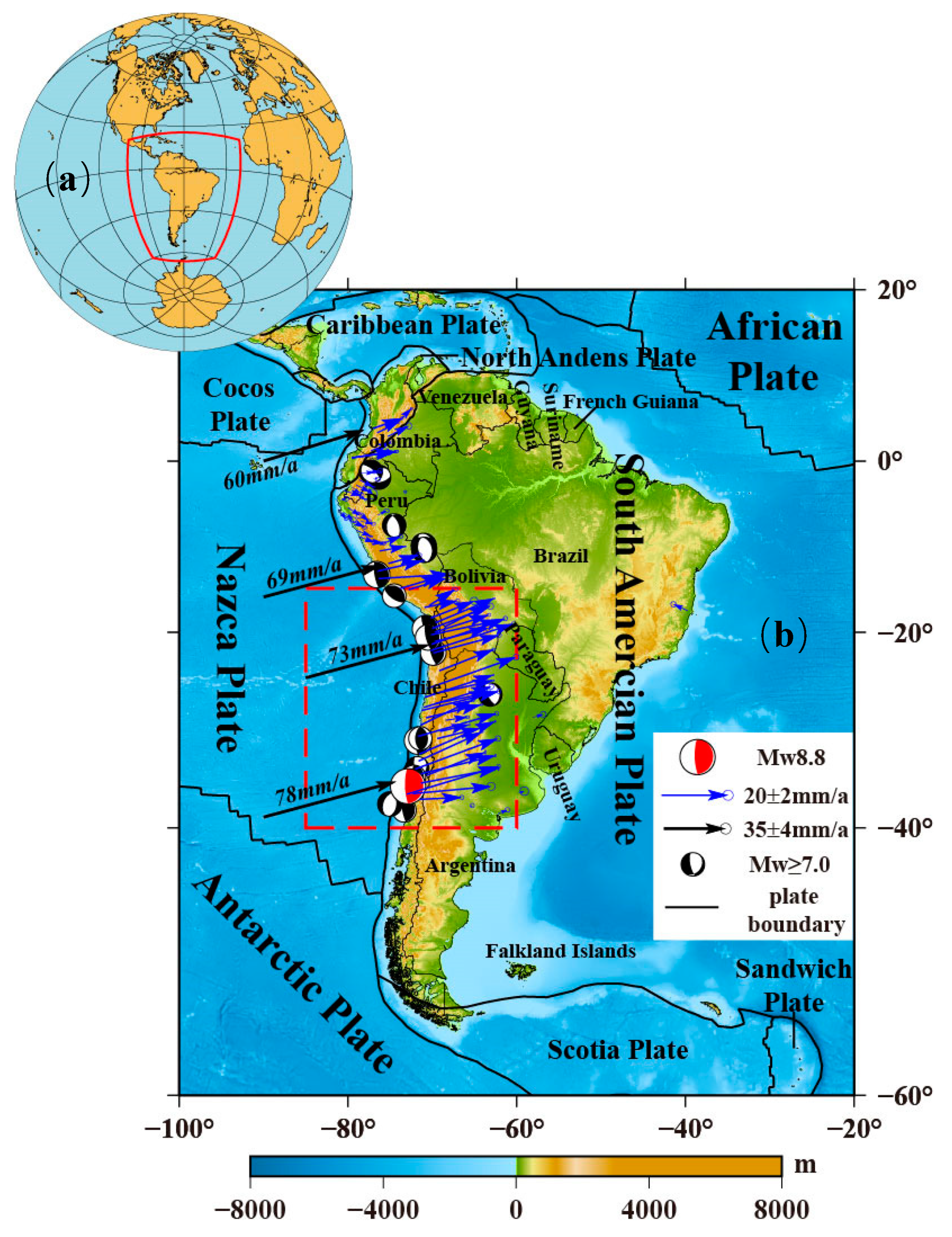
2. Tectonic Background

Chile is located in the Andean subduction zone, where the Pacific and the South American plates collide (Figure 1). Chile is also one of the countries that has suffered the most harm from earthquakes [27,28]. The Nazca plate, which belongs to the eastern margin of the Pacific plate, is subducted beneath the South America plate with a convergence speed of ~80 mm/year in the southern region and ~65 mm/year in the northern region along the subduction zone [29]. Although the rate of subduction varies little along the entire arc, there are complex changes in the geologic processes along the subduction zone that dramatically influence tectonic activities along the western edge of South America [30]. The plate convergence in the subduction zone is mainly manifested by the sliding of the plate contact surface on the thrust belt and the shortening of the continental lithosphere in the South America plate. The plate subduction has led to not only the uplift of the Andes, but also the thickening of the margin crust of the South America plate [31]. In addition, the South American subduction zone and the South American plate are also squeezed by the expansion of the mid-Atlantic ridge, are affected by the dynamics of the Caribbean plate in the north, and are pushed by the Antarctic plate in the southwest. The combined actions of these surrounding plates lead to severe and complex deformation of the South American plate and strong seismic activity on its western edge [32,33,34].

Due to the continuous eastward subduction of the Nazca plate, the collision zone between the Nazca and South American plates is a natural site for the brewing and occurrence of large earthquakes and volcanic activity. The Chile subduction zone is among the most active convergent margins on earth, producing a large earthquake (Mw > 8.0) every ~10–20 years. Most of the large earthquakes in South America are constrained to shallow depths of 0–70 km as a result of both crustal and interplate deformation. Crustal earthquakes are caused by deformation and mountain building in the overriding South America plate and can be as deep as approximately 50 km. Interplate earthquakes occur due to slip along the dipping interface between the Nazca and the South America plates [30]. The 2010 Mw 8.8 Maule Chile earthquake occurred in the south-central region of the subduction of the Nazca plate underneath the overlying South American plate [35]. This earthquake hit the south-central part of Chile producing a tsunami which affected not only the continental central Chilean coast, but also the Juan Fernández Islands located some 670 km offshore. The rupture zone, estimated from aftershock distribution, covers a distance of approximately 500 km long. Based on the global earthquake catalogue from the United State Geological Survey (USGS), this earthquake is the fifth strongest earthquake since 1900 as well as the third greatest earthquake with Mw ≥ 8.5 since 2004. The maximum fault slip of this earthquake was about 6–7 m, and the ruptured region stretched ~500 km along the South Chilean subduction zone reference. In addition, the Chilean coastal belt has generated several of the largest earthquakes ever recorded (>Mw 7.5,

Table 1. Some typical largest earthquakes ever recorded (>Mw 7.5) around the Chilean coastal belt.

Date (UTC)	latitude/S	Longitude/W	Magnitude/Mw	Rupture Scale/km	Location	References
8 July 1730	32.5	71.5	9.1–9.3	600–800	Valparaiso	[37]
20 February 1835	36.8	73.0	8.5	300	Concepcion	[38]
10 May 1877	19.6	70.2	8.5	420	Iquique	[39]
3 March 1985	33.1	71.9	7.8	240	Santiago	[40]
17 August 1906	32.4	71.4	8.2	200	Valparaiso	[41]
11 November 1922	28.3	69.8	8.5	300	Copiapo	[42]
6 April 1943	31.4	71.5	7.9	220	Coquimbo	[43]
22 May 1960	38.2	73.1	9.6	800	Valdivia	[44]
3 April 2014	19.59	70.73	8.1	200	Iquique	[45]
16 September 2015	31.64	71.74	8.3	200	Illapel	[46]

).

3. Methods and Data

3.1. Gravitational Field Changes

The spherical harmonic expansion of the gravitational potential of the Earth is the basis for studying various characteristics of its gravitational field. According to the spherical harmonic expansion theory, the external gravitational potential of the Earth can be expressed as follows [47,48,49]:

$$\mathrm{V}\left(r,\theta ,\lambda ,t\right)=\frac{GM}{r}+\frac{GM}{r}\left[{\displaystyle \sum }_{l=2}^N{(\frac{a}{r})}^l{\displaystyle \sum }_{m=0}^l\left(C_{lm}\left(t\right)cosm\lambda +S_{lm}\left(t\right)sinm\lambda \right){\overline{P}}_{lm}\left(cos\theta \right)\right]$$

(1)

where $V\left(r,\theta ,\lambda ,t\right)$ is the external gravitational potential related to the changes of spatial position and time; $\left(r,\theta ,\lambda \right)$ represents the radial coordinate, colatitude, and longitude in a spherical coordinate system; $t$ is time; $G$ is the gravitational constant, $M$ is the mass of the Earth; $GM$ is the gravitational constant; $r$ is the mean equatorial radius of the Earth; a is the equatorial radius of the Earth; $C_{lm}\left(t\right)$ and $S_{lm}\left(t\right)$ are fully normalized time-varying spherical harmonic coefficients; and ${\overline{P}}_{lm}\left(\cos \theta \right)$ is a fully-normalized associated Legendre functions with order $l$ and degree $m$.

When studying the long-time sequence of a time-variable gravitational field, the average gravitational field over a period is usually selected as the background field. Then, the monthly time-variable gravitational field model can be expressed relative to the background field. The ellipticity and topography of the Earth have weak influence on the variation of low-order gravitational field over time and therefore, the monthly gravitational field changes can be further represented on a spherical surface of radius R (Equation (2)), which can be approximately considered to be the changes of the gravitational field on the surface of the Earth [48,50]:

$$\mathsf{\Delta }g\left(\theta ,\lambda \right)=\frac{GM}{R^2}{\displaystyle \sum }_{l=2}^N\left(l+1\right){\displaystyle \sum }_{m=0}^l\left(\mathsf{\Delta }{C}_{lm}\cos m\lambda +\mathsf{\Delta }{S}_{lm}\sin m\lambda \right)·{\overline{P}}_{lm}\left(\cos \theta \right)$$

(2)

where $\mathsf{\Delta }g\left(\theta ,\lambda \right)$ is the change in gravity.

3.2. First-Order GGCs

If we set a local rectangular coordinate system established at any points on the surface of the Earth, where the X axis points to the north, the Y axis points to the east, and the Z axis points downward toward the center of the earth. Then, by deducing the first partial derivative of Equation (2) with respect to $\mathsf{\theta }$, $\mathsf{\lambda }$, and $\mathrm{r}$, respectively, the components of the first-order GGCs along the three coordinate axes can be obtained [47,51,52]:

$$\mathsf{\Delta }{g}_X\left(\theta ,\lambda \right)=\frac{GM}{R^3}{\displaystyle \sum }_{l=2}^N\left(l+1\right){\displaystyle \sum }_{m=0}^l\left(\mathsf{\Delta }{C}_{lm}\cos m\lambda +\mathsf{\Delta }{S}_{lm}\sin m\lambda \right)·\frac{d\left[{\overline{P}}_{lm}\left(\cos \theta \right)\right]}{d\theta }$$

(3)

$$\mathsf{\Delta }{g}_Y\left(\theta ,\lambda \right)=\frac{GM}{R^3}{\displaystyle \sum }_{l=2}^N\left(l+1\right){\displaystyle \sum }_{m=0}^{l}m\left(-\mathsf{\Delta }{C}_{lm}\sin m\lambda +\mathsf{\Delta }{S}_{lm}\cos m\lambda \right)·\frac{{\overline{P}}_{lm}\left(\cos \theta \right)}{\sin \theta }$$

(4)

$$\mathsf{\Delta }{g}_Z\left(\theta ,\lambda \right)=\frac{GM}{R^3}{\displaystyle \sum }_{l=2}^N\left(l+2\right)\left(l+1\right){\displaystyle \sum }_{m=0}^l\left(\mathsf{\Delta }{C}_{lm}\cos m\lambda +\mathsf{\Delta }{S}_{lm}\sin m\lambda \right)·{\overline{P}}_{lm}\left(\cos \theta \right)$$

(5)

3.3. GRACE Data

We selected the monthly gravitational field models with the highest order of 60, where the spherical harmonic coefficients were obtained from the Release 06 (RL06) Level 2 version issued by the University of Texas Center for Space Research (CSR). We used 174 monthly gravitational field models from January 2003 to March 2016 and June 2018 to August 2019 to study the temporal and spatial gravity changes among the pre-seismic, co-seismic, and post-seismic stages of the 2010 Mw 8.8 Maule Chile earthquake. The degree 02 (C20) term of the spherical harmonic coefficients was replaced by their corresponding ones estimated using satellite laser ranging data [53]. Due to the influence of the near polar orbit design of the satellite [54], GRACE cannot observe the geocentric motion very well. Monthly geocenter estimates calculated by Sun [55] were used to account for the degree-1 coefficients of the gravity field. These coefficients, which have been normalized using the GRACE standards, represent the degree-1 gravity coefficients that should be added to the GSM coefficients to correct for geocenter motion. During the process of calculating the gravitational field changes, the P3M6 method [17,56] was used to remove the correlation between the odd- and even-order spherical harmonic coefficients in the spherical harmonic domain, and the 300 km Gaussian smoothing method was further adopted to reduce the high-order spherical harmonic coefficient noise to weaken the influence of the north–south stripes. The 300 km Gaussian smoothing method was also adopted to optimize the gravity gradients changes.

The gravitational field observed by GRACE may be affected by hydrological factors, which will influence the analysis of geodynamics-related information [48]. We further employed the grid data ($2.5°\times 2.5°$) from the Global Land Data Assimilation System by using the same processing strategy as for the GRACE gravity data to extract hydrological data, which were further subtracted from the observations to deduce the hydrological impact [22,23].

4. Results and Analysis

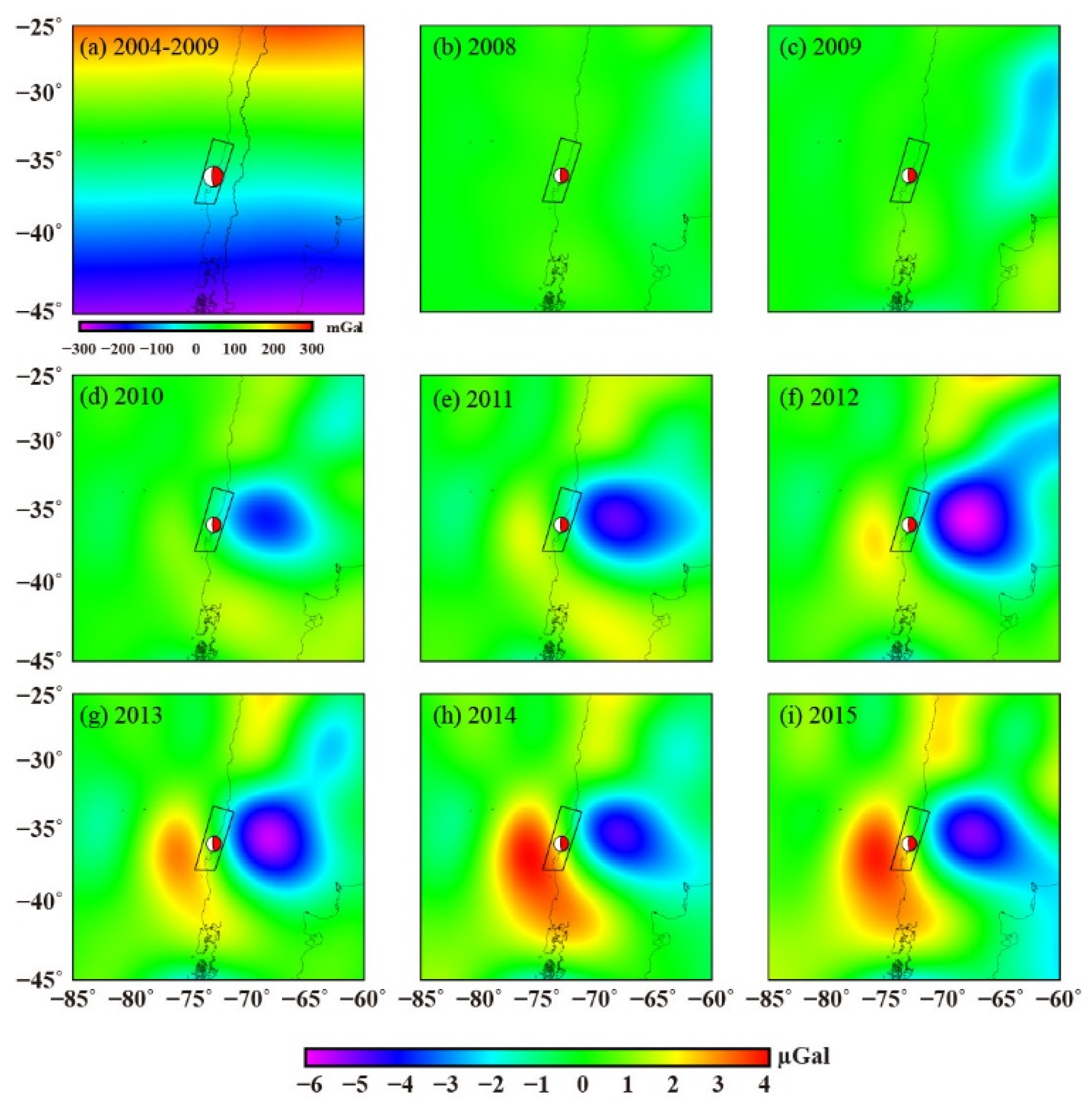
4.1. Long-Term Gravity Changes

Seventy-two continuous monthly gravitational field models from January 2004 to December 2009 were selected as the background field (Figure 2a), and the average annual total gravitational field changes (including the co-seismic gravity changes) from 2008 to 2015 were calculated to obtain the spatial variations of the long-term (from 2008 to 2015) gravitational field in the Chilean area (Figure 2).

Figure 2 shows that in 2010, the year of the Mw 8.8 Chile earthquake, two obvious gravity signals with opposite characteristics appear on the hanging wall and footwall of the seismogenic fault (Figure 2d). The footwall presents ~1.6 μGal positive gravity changes, while the hanging wall shows ca. −3.9 μGal negative gravity changes. Between 2011 and 2015, the positive and negative gravity changes around the two sides of the seismogenic fault all exhibit significant differences (Figure 2e–i). The positive gravity changes and their scopes in the footwall increase year-by-year (Figure 2e–i). The scopes of the negative gravity changes in the hanging wall overall show a gradually decreasing trend year-by-year (although the scope relatively lager in 2012) (Figure 2e–i). However, the gravity changes are relatively flat between 2008 and 2009 (Figure 2b,c).

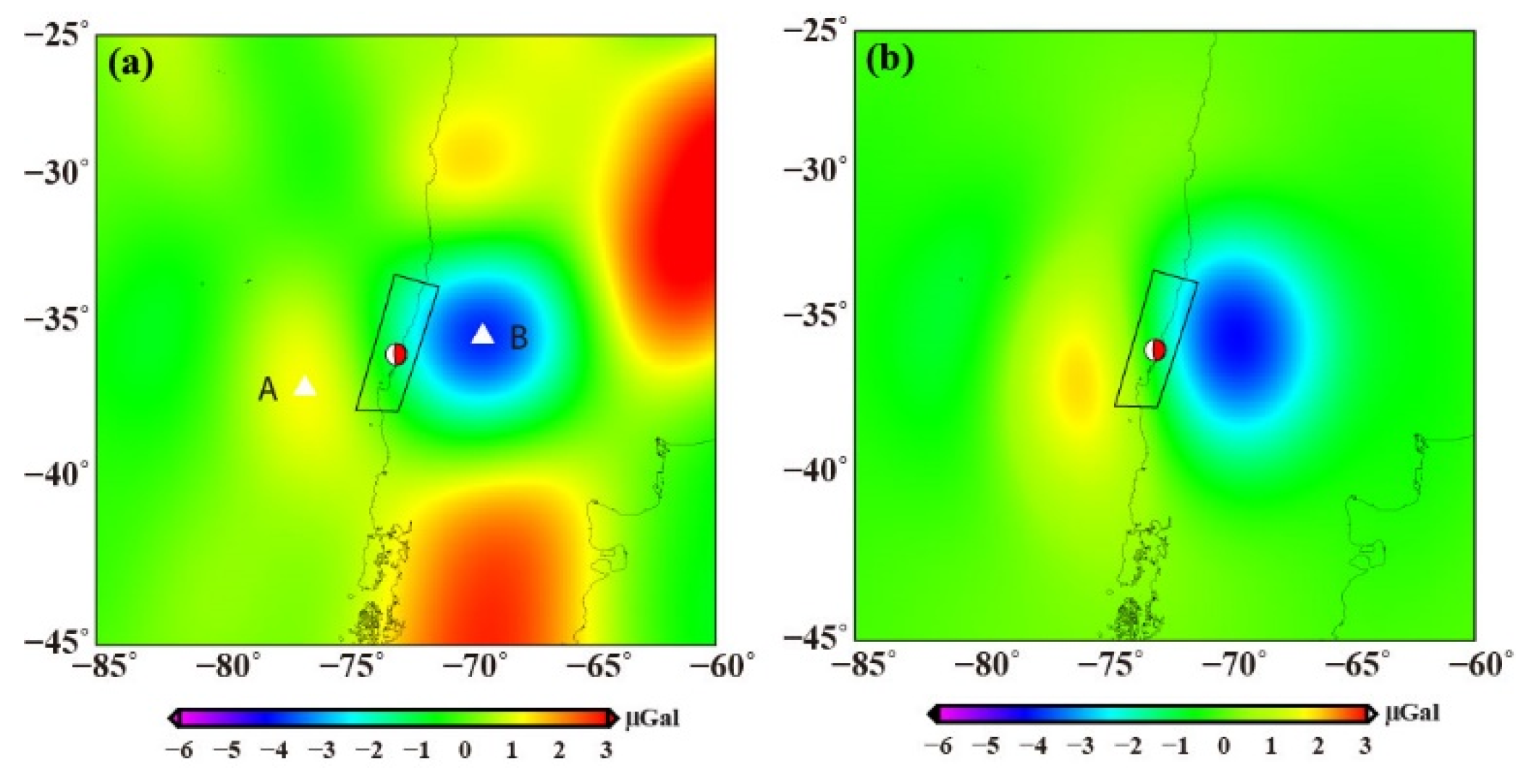
4.2. Co-Seismic Gravity Changes

To investigate the spatial variations of the co-seismic gravitational field caused by the 2010 Mw 8.8 Maule Chile earthquake, we used average gravitational field models for a period of ca. one year, spanning both the pre-seismic (form February 2009 to January 2010) and post-seismic (form March 2010 to February 2011) stages (Figure 3a).

The co-seismic gravity changes of the earthquake present significant positive and negative differential changes on the two sides of the seismogenic fault. The positive gravity change reaches ~1.2 μGal on the footwall (subducting plate), while the negative gravity change reaches about −4.0 μGal on the hanging wall (thrusting plate). The peak-to-trough amplitude of the co-seismic gravity changes reaches ~5.2 μGal. We also used the spherical dislocation model [57] with five-segment parameters [58] to calculate the theoretical co-seismic gravity changes. It should be noted that for earthquakes under oceans, gravity changes on the ocean part may be influenced by seawater disturbances produced by the displacement of the seabed. Therefore, it was necessary to perform seawater quality correction of the gravity changes on the ocean part [57]. Additionally, the calculation results from the dislocation model were processed through a 300 km Gaussian filter in the spatial domain for comparison with the gravity changes observed by GRACE (Figure 3b).

The gravity changes calculated using the dislocation model also show significant positive and negative gravity differential changes on the two sides of the seismogenic fault, with ~1.9 μGal positive gravity changes on the footwall and ca. −4.2 μGal negative gravity changes on the hanging wall (Figure 3b). The maximum change in amplitude in the theoretical calculations performed using the dislocation model is smaller than that observed by GRACE (Figure 3a,b). The reasons for the difference may be the simplicity of theoretical fault model and noise background. In addition, the GRACE observations contained the mixed co-seismic and post-seismic signals [50]. However, it is also evident that the overall trends of the gravity changes according to the theoretical calculations and GRACE observations are consistent (Figure 3a,b).

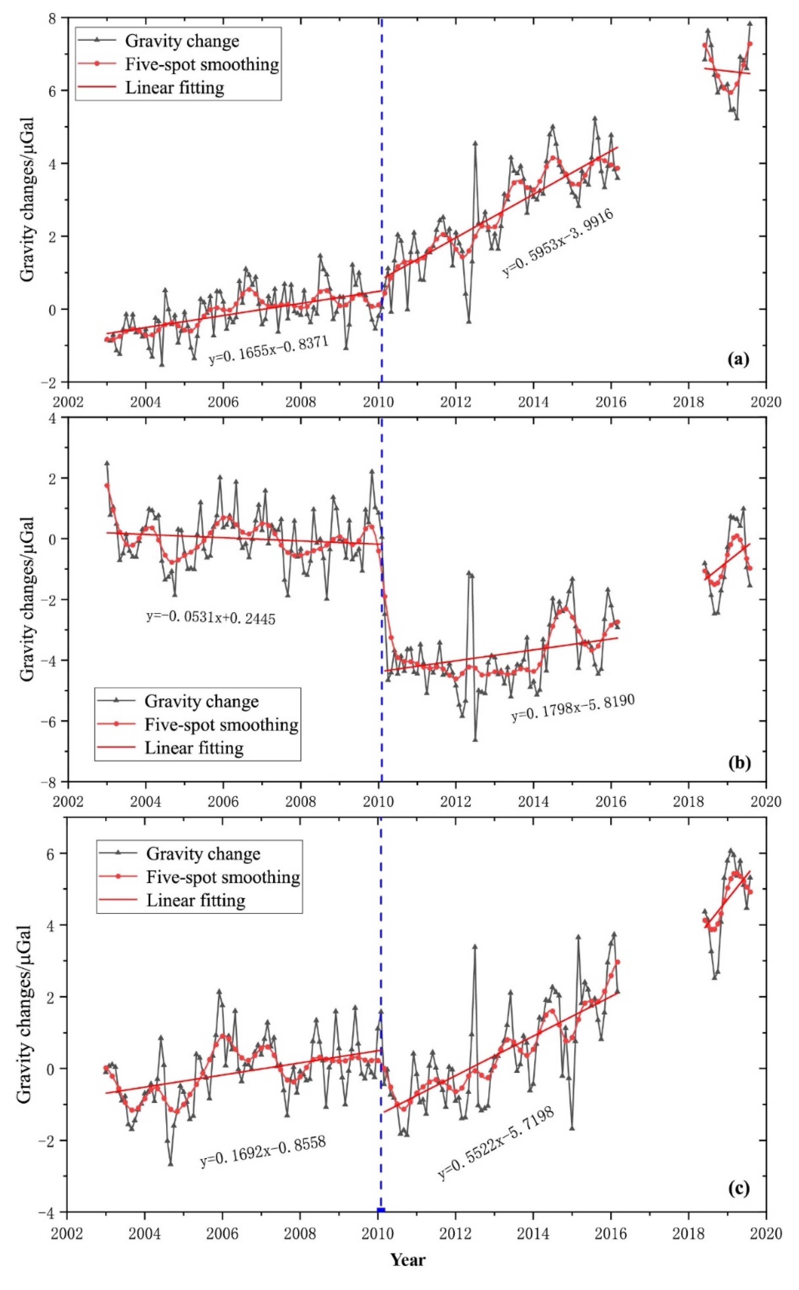
4.3. Time Series of Gravity Changes

The time series of the gravity at key points can more clearly and quantitatively reflect the local gravity variations. Therefore, we selected three key points: points A (37.2°S, 76.6°W) and B (35.5°S, 69.4°W), which have the maximum and minimum gravity changes in Figure 3a (white triangles), and the epicenter (36.1°S, 72.9°W) to investigate the temporal variation characteristics of the gravitational field in further detail.

To display the trends of the time series more clearly, we deduced the annual and semi-annual cyclical effects, using cubic spline interpolation to complement the missing data, and adopted five-point smoothing combined with the least-squares fitting to obtain the final time series of the long-term gravity changes at the key points (Figure 4a–c). The gravity changes at all three key points exhibit obvious jumps on February 27, 2010, the date of the Mw 8.8 Chilean earthquake (Figure 4a–c). The magnitude of the co-seismic gravity change at point A (on the footwall of the seismogenic fault) reaches ~1.1 μGal, and that at point B (on the hanging wall) reaches ~4.7 μGal (Figure 4a,b). The least squares line fitting of the gravity changes curve at point A are around 0 μGal before the earthquake and exhibit an obvious increase in the positive gravity change after the earthquake. Although the fluctuation of the gravity changes at point B is greater than that at point A before the earthquake, The least squares line fitting of the gravity changes curve also are around 0 μGal; however, they exhibit significant negative gravity variations with an increasing trend after the earthquake. The overall gravity variations on the hanging wall of the seismogenic fault are stronger than those on the footwall, which has features similar to those of the 2004 Sumatra Mw 9.3 earthquake [50].

The amplitude of the gravity changes of the epicenter varies from −2 μGal to 4 μGal (2003–2016). The gravity changes of the epicenter show overall increasing trends before and after the earthquake, in particular, a rapid increasing trend after the earthquake (Figure 4c). However, we found the increasing rate before the 2010 Mw 8.8 earthquake is not obvious (Figure 4c).

Figure 4 shows that the gravity changes at key points before the earthquake are also relatively large. We therefore investigated earthquakes (Mw > 6.0) in the pre-seismic period around the key points, including the largest Mw 7.0 O’Higgins earthquake on February 27, 2010 (34.3°S, 71.8°W). However, it is difficult to conclude that the larger gravity changes in pre-seismic period were directly related to these smaller magnitude earthquakes. The gravity changes observed by GRACE are mainly caused by tectonic deformation, underground material flow and groundwater storage changes. There are no large rivers or glaciers in the earthquake area and the significant gravity anomalies are distributed along the tectonic deformation zone, which indicate that the gravity changes may contain the density changes caused by the migration of underground materials and the deformation caused by the tectonic movement. In addition, due to the characteristics of the structural location of Chile, the influencing factors of gravity changes and surface deformation are very complicated. Moreover, since GRACE detected the gravity change signal associated with the Sumatra earthquake, scientists have been exploring whether GRACE can detect the gravity change signal produced by an earthquake smaller than the Sumatra earthquake [16,59,60]. Gross and Chao used the normal model solution of free oscillation of the earth to prove that GRACE can detect large earthquakes [59]. Theoretically, the co-seismic gravity variation of a shear source larger than M 9.0 or a tension source larger than M 7.5 should be detected by GRACE [16,60]. Since earthquakes normally contain both sheer and tensional/compressional components, theoretically, an earthquake with M > 8 may be detected by GRACE [16,60].

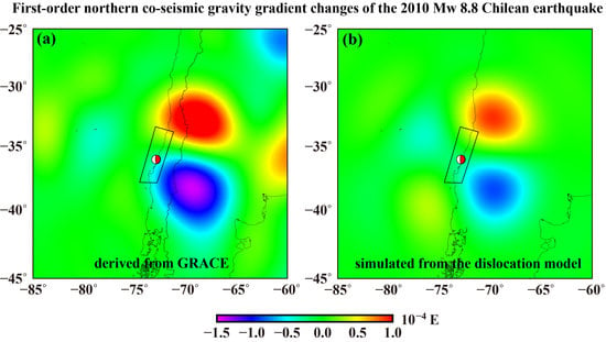
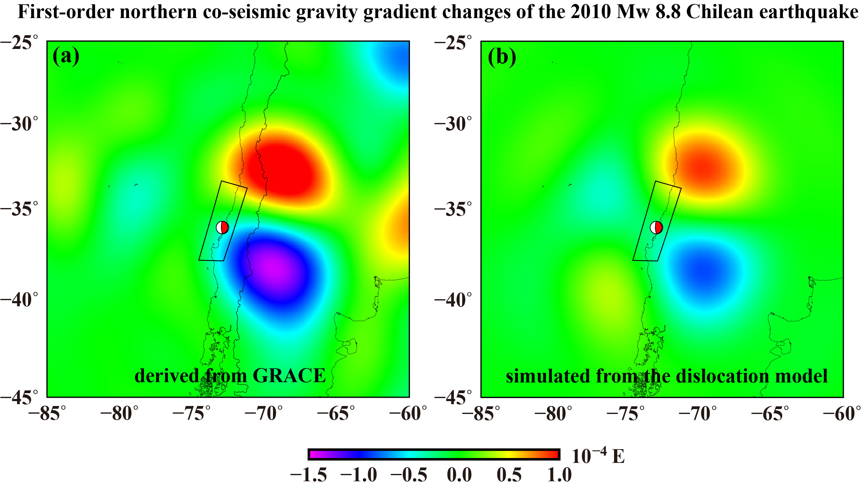
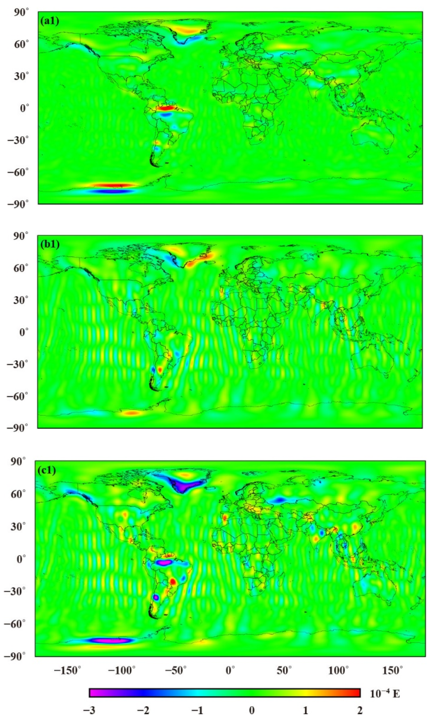
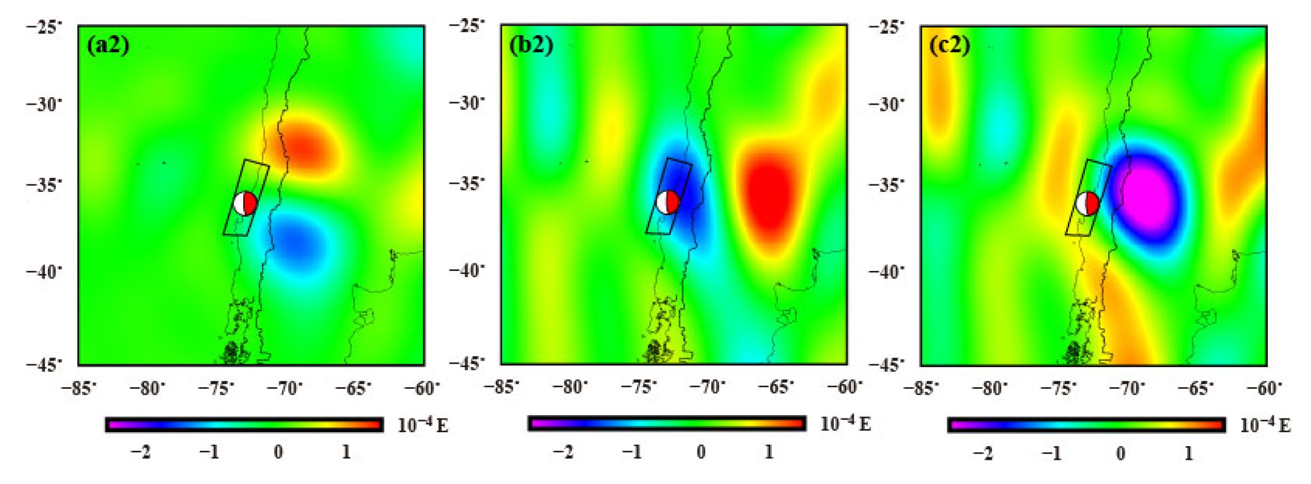
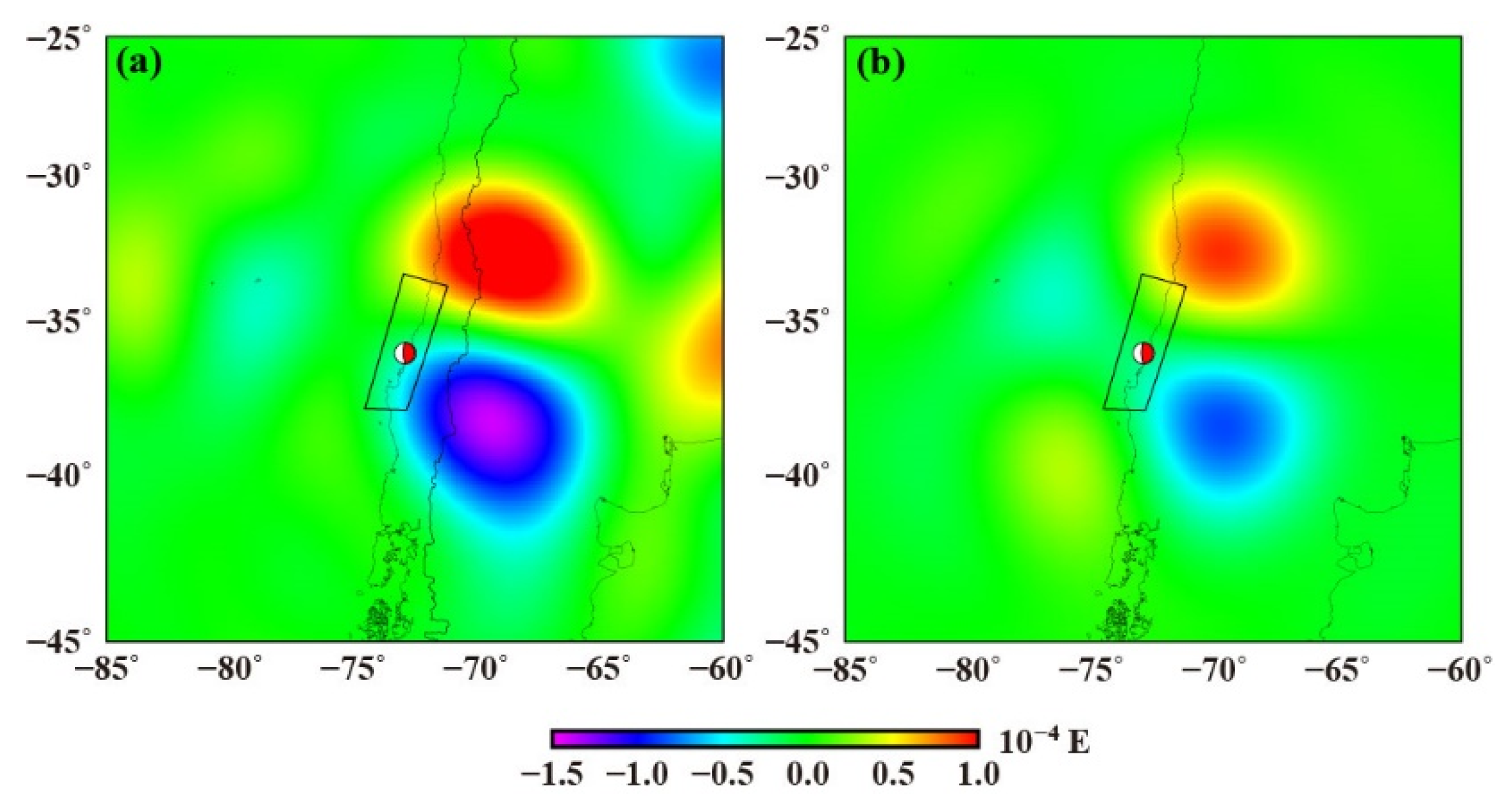
4.4. First-Order Co-Seismic GGCS

According to the principle described in Section 3.2, we used Gaussian filtering with a window of 300 km to calculate the co-seismic northward (Figure 5a2), eastward (Figure 5b2), and vertical GGCs (Figure 5c2). Figure 5a2,b2 show obvious spatial changes of the horizontal GGCs with positive–negative–positive characteristics especially in the northward, whereby the different dividing lines strike between the positive and negative zones. The epicenter is located in the middle of the negative change zone. The range of the northward co-seismic GGCs is from −1.4 × 10⁻⁴ E to 1.3 × 10⁻⁴ E (Figure 5a2), while the eastward co-seismic GGCs is larger than the northward one, ranging from −1.8 × 10⁻⁴ E to 1.8 × 10⁻⁴ E (Figure 5b2). The vertical GGCs show details of the co-seismic gravity changes and exhibit obvious spatial changes with approximately negative–positive–negative characteristics, whereby the magnitude is slightly larger than that of the horizontal GGCs.

Due to the limitations of GRACE satellite observations themselves (hybrid effects of satellite orbit errors and correlated errors of Stokes coefficients), oceanic and atmospheric model errors, the time-varying gravity field models obtained by GRACE have obvious north–south oriented high-frequency strip errors [17,56]. To reduce these artifacts, a Gaussian filter, decorrelated filter, Fan filter and other filters can be adopted. Here we only used 300-km Gaussian filtering to show the suppressive effect of the first-order northern co-seismic GGCs on the north–south strip error without decorrelation filtering. However, a single filter has its limitations, thus, there are residual stripes in Figure 5, especially in Figure 5b1,c1

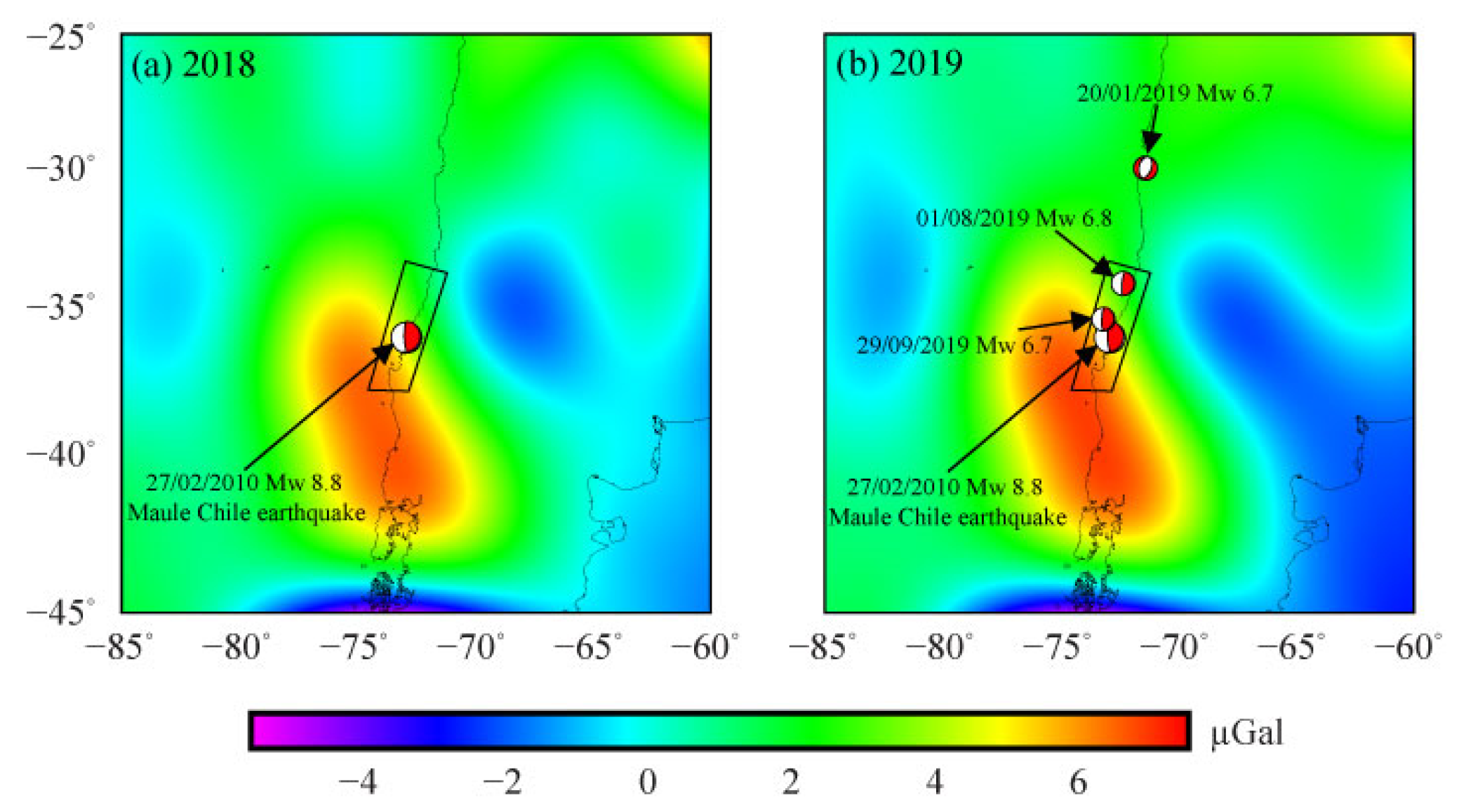
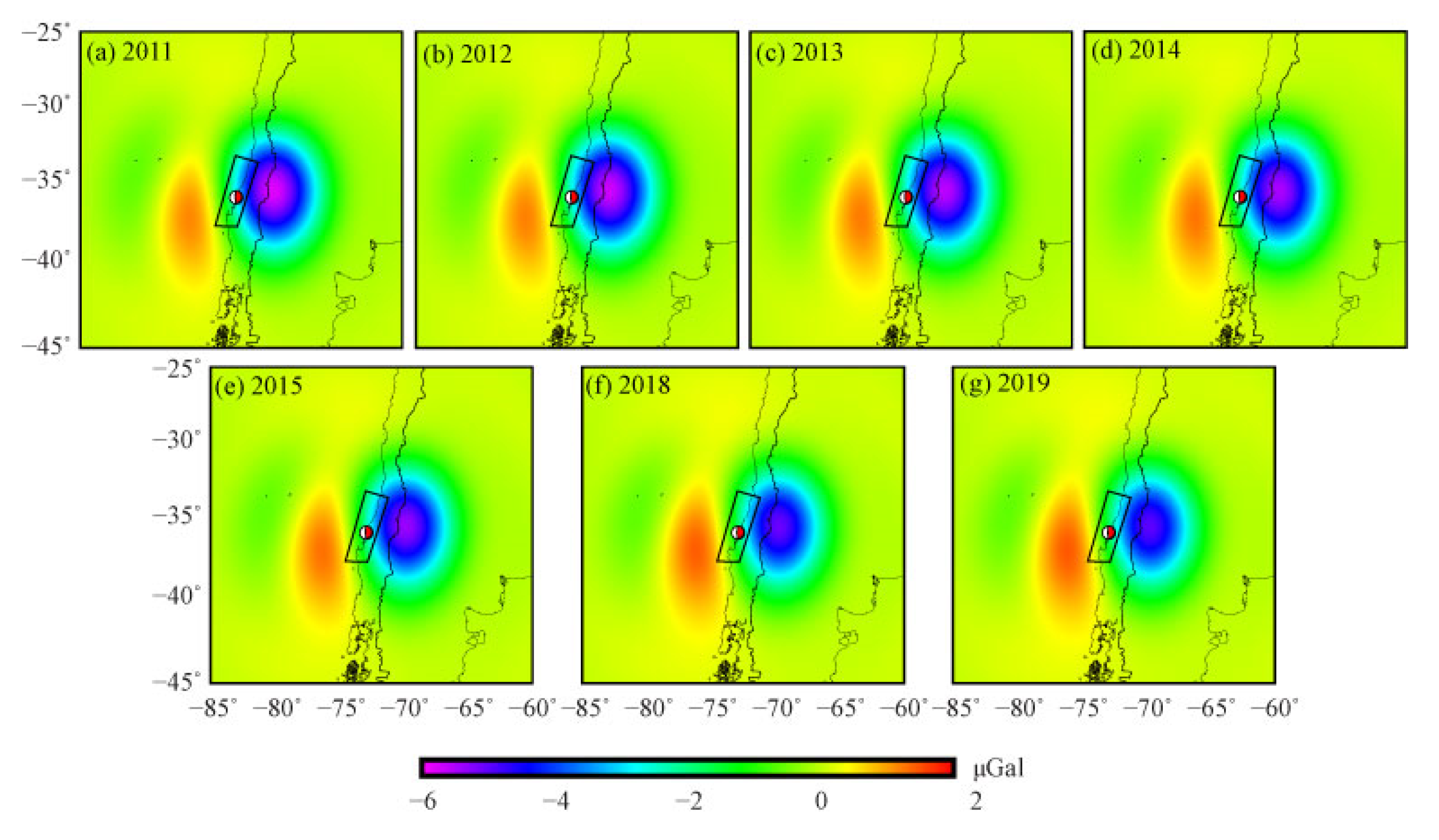
4.5. Latest Post-Seismic Gravity Changes Revealed by GRACE-FO

On May 22, 2018, the GRACE-FO satellites were launched and the new GRACE-FO data were subsequently provided. We selected the monthly gravitational field models with a highest order of 60, where the spherical harmonic coefficients were obtained from the Release 06 (RL06) Level 2 version issued by CSR. We used 15 monthly gravitational field models of GRACE-FO from June 2018 to August 2019 to study the spatial gravity changes of the post-seismic stages of the 2010 Mw 8.8 Maule Chile earthquake (Figure 6), and adopted the same background data with GRACE.

During 2018 (Figure 6a) and 2019 (Figure 6b), the gravity changes of the Chile region exhibit obvious inherited development characteristics, both temporally (Figure 4) and spatially (Figure 2), which have two obvious gravity signals with opposite characteristics appear on the hanging wall and footwall of the seismogenic fault. It should be noted that between 2010 and 2019, the positive gravity changes of the footwall exhibit a significant enhanced trend and the scope is also expanding, while the extent of the negative gravity changes in the hanging wall show a gradually decreasing trend. The time range of selected GRACE-FO data is between June 2018 and August 2019, there were no large earthquakes of Mw ≥ 7.0 but there have been four earthquakes of Mw ≥ 6.5 (GCMT, the red focal mechanism ball in Figure 6b). However, there is no significant difference among Figure 6a,b and Figure 2b–f. This feature indicates that the Chile area currently still be mainly affected by the post-seismic effect of the 2010 Mw 8.8 Maule Chile earthquake.

5. Discussion

5.1. Comparison with Previous Co-Seismic Gravity Changes Observed by GRACE

The co-seismic gravity changes of the 2010 Mw 8.8 Maule Chile earthquake have been studied in several studies based on GRACE data [1,24,25,26,61]. The features and trends of the co-seismic gravity changes obtained in our study are similar to the previous results, but also have certain differences in terms of the detailed spatial distribution and the magnitude of the gravity changes (

Table 2. Comparison of co-seismic gravity changes of the 2010 Mw 8.8 Chilean earthquake obtained by different researchers.

Scientist	Physical Quantity	Observation Data Dislocation Model	Time Scale	Filtering	Spatial Distribution	Magnitude (Gravity/μGal)
[26]	Co-seismic gravity change	GRACE data issued by CSR Release 04 (RL04) Level 2	Three months before and after the earthquake	P3M6+300 km Gaussian filter	Positive–negative	−5–+2
		Spherical dislocation model		300 km Gaussian filter	Positive–negative	−8.9–+3.9
[24]	Co-seismic gravity change	GRACE data issued by CSR Release 04 RL04 Level 2	Three months before and after the earthquake	P3M15+300 km Gaussian filter	Negative	Largest drop of ~−5
		Spherical dislocation model		300 km Gaussian filter	Negative	Largest drop of ~−5
[1]	Co-seismic gravity change	GRACE data issued by CSR Release 04 RL04 Level 2	One year before and after the earthquake	Slepian function	Positive–negative	−10–+2
[61]	Co-seismic gravity change	GRACE data issued by CSR RL04 Level 2	One year before and after the earthquake	P3M6+300 km Gaussian filter	Positive–negative	−4.5–+0.7
		Rectangular dislocation model		300 km Gaussian filter	Positive–negative	−6.3–+2.4
[25]	Co-seismic gravity change	GRACE data issued by JPL Level-1B	Two weeks before and after the earthquake	500 km Gaussian filtering	Positive–negative	−5 to the east of the epicenter
This study	Co-seismic gravity change	GRACE data issued by CSR Release 06 RL06 Level 2	One years before and after the earthquake	P3M6+300 km Gaussian filter	Positive–negative	−4.0–+1.2
		Spherical dislocation model		300 km Gaussian filter	Positive–negative	−4.2–+1.9

). We obtained co-seismic gravity changes of −4.0–1.2 μGal based on GRACE data of one year bracketing the earthquake, while Wang et al. [1] and Li [60] obtained co-seismic gravity changes of −10–2 μGa and −4.5–0.6 μGal during the same time span, respectively. Heki and Matsuo [24] and Zhou et al. [26] obtained a co-seismic gravity change of −5 μGa and −5–2 μGal based on three months of GRACE data before and after the earthquake, respectively. Han et al. [25] obtained a co-seismic gravity change of −5 μGal to the east of the epicenter based on GRACE data of two weeks. A detailed comparison of the results is provided in Table 2.

The reasons of the differences in terms of the detailed distribution and the magnitude of the gravity changes among these studies may include the following. First, different time spans of GRACE data were used and, accordingly, the observed gravity changes reveal the earthquake deformation during different times. Second, different filtering methods with different resolutions were introduced to the processing of the GRACE data, which can affect the final gravity field results. For example, Wang et al. [1] mainly used the Slepian function, while Li [61] used the P3M6 plus 300 km Gaussian filter based on the same time scale (one year before and after the earthquake). Heki and Matsuo [24] used P3M6 plus 300 km Gaussian filter while Zhou et al. [26] used P3M15 plus 300 km Gaussian filter; both were based on the same time scale (three months before and after the earthquake). Third, the different datasets issued from different organizations (along with different inversion method for data processing) were used to analyze the gravity changes. For example, Han et al. [25] adopted the GRACE data issued by JPL Level-1B while others used data from CSR. Lastly, different releases of GRACE data even from the same organization were used to analyze gravity changes, and the data quality and accuracy from the newer version are generally improved compared with the previous version. For example, the version of GRACE data used in our study is RL06 Level 2 from CSR, while Li [61] used the CSR’s RL04 Level 2 products based on the same time scale. The difference in the modeled co-seismic gravity changes among these studies are due to the different fault parameters and different types of dislocation models, such as the rectangular dislocation model [61] and the spherical dislocation model [24,26]. In summary, the discrepancy in gravity changes obtained by GRACE among the different studies is due to the difference in data time spans, filtering methods, data providers, released versions, and fault parameters and types of dislocation models.

In this study, the co-seismic gravity changes of the 2010 Mw 8.8 Maule Chile earthquake were obtained based on the newest version Release 06 (RL06) Level 2 of GRACE data issued by CSR. Compared to the version Release 05 (RL05) Level 2, there are improvements in the background gravity field, the third body perturbation, the solid Earth polar tide model, and the atmospheric and non-tidal modes in the Release 06 (RL06) Level 2 version.

5.2. Advantages of the First-Order Northern Co-Seismic GGCs in Detecting Co-Seismic Signals

In order to effectively eliminate noise, when using the GRACE data to study the co-seismic gravity changes, decorrelation filtering is often performed; however, this also weakens or distorts the real signal while eliminating the error. In this study, we attempted to directly use 300 km Gaussian filtering without decorrelation filtering, and obtained the first-order GGCs of three components (Figure 6). It can be seen from the comparison of the global distribution that the north-south strip phenomenon in the distribution of GGCs in the northern direction is smoother than that in the eastern and vertical directions (Figure 5a1,b1,c1). For the vertical global distribution, the reason for the obvious north-south strip may be that the term $\left(\mathrm{l}+2\right)\left(\mathrm{l}+1\right)$ in the spherical harmonic display (Equation (5)) not only amplifies the signal, but also amplifies the error. However, although the gravity gradient will amplify short-wave noise while highlighting the small-scale signal, the interference from the north-south strip error is significantly less than the gradient components in the other two directions due to the suppression effect of the northward gradient on the error. The advantage of the northern gravity gradient may be derived from the near-polar flight orbit of the GRACE satellites, such that the observation sensitivity in the north-south direction is higher than in other directions; thus, the signal-to-noise ratio of the measurement results in the north-south direction is higher.

Figure 7 shows a comparison between the northern co-seismic GGCs (Figure 7a) and theoretical northern co-seismic GGCs simulated by the dislocation model (Figure 7b, corresponding to Figure 4). Both are in good agreement with each other in terms of the spatial distribution and variation amplitude (Figure 7a,b). Moreover, the coincidence degree is better than that of the gravity changes (Figure 3 versus Figure 4), which further demonstrated the superiority of the northern co-seismic GGCs in extracting the co-seismic signal.

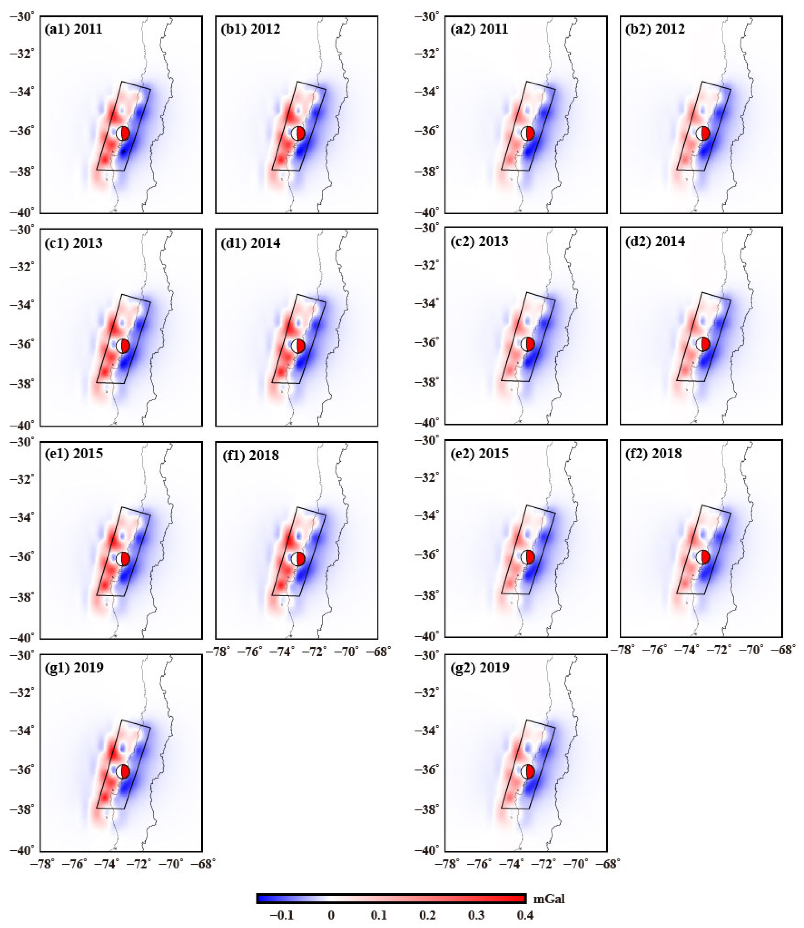
5.3. Post-Seismic Gravity Changes Simulated by Viscoelastic Dislocation Model

In order to further study the internal mechanism of post-seismic gravity changes of the 2010 Mw 8.8 Maule Chile earthquake, we numerically simulated the gravity change of the earthquake based on the dislocation theory. The dislocation theory used in this study is based on the viscoelastic earth model, which has been successfully used in the simulation of co-seismic and post-seismic gravity changes [62]. The program used in the calculation is the viscoelastic dislocation calculation program PSGRN/PSCMP developed by Rongjiang Wang of the German Geosciences Center (GFZ) [62]. The fault model used in the viscoelastic dislocation model is the same as the model mentioned in Section 4.2. The parameters of the earth model used in this study are shown in

Table 3. The parameters of earth model used in viscoelastic dislocation model (based on the CRUST 1.0 model).

$\mathbf{Depth}\left(km\right)$	$\mathbf{Density}\left({10}^{3}kg·m^{-3}\right)$	$\mathbf{P}\mathbf{Wave}\mathbf{Velocity}\left(km·s^{-1}\right)$	$\mathbf{S}\mathbf{Wave}\mathbf{Velocity}\left(km·s^{-1}\right)$	$\mathbf{Viscosity}\left({10}^{19}Pa·s\right)$
0–0.66	1.82	1.75	0.34	∞
0.66–11.93	2.72	6.00	3.50	∞
11.93–23.21	2.86	6.60	3..80	∞
23.21–34.83	3.03	7.20	4.10	∞
34.83–6371	3.30	8.00	4.45	1.0

.

In order to compare the simulated gravity variation of the modelling with the observation of GRACE, it is necessary to restore the calculated value of the modelling to the fixed point in space after spatial correction. The space correction can be expressed as [63]:

$$\mathsf{\Delta }g\left(\theta ,\lambda \right)=\delta g\left(\theta ,\lambda \right)+\beta ·u_z\left(\theta ,\lambda \right)$$

(6)

where $\mathsf{\Delta }g\left(\theta ,\lambda \right)$ is the gravity change at a fixed point in space, $\delta g\left(\theta ,\lambda \right)$ is the gravity variation of the Earth’s surface calculated by dislocation model, and downward represents positive; $u_z\left(\theta ,\lambda \right)$ is the vertical deformation of the surface calculated by the dislocation model, and upward represents positive; $\beta$ is the vertical gravity gradient at the surface: $\beta =2gR/R$, where $R$ is the average radius of the Earth, and $g$ is the average gravity value of the Earth’s surface.

Furthermore, in the study of seafloor earthquake (like the 2010 Mw 8.8 Maule Chile earthquake), it must consider the compensation effect of sea water on co-seismic deformation, to correct the effect of sea water quality (Figure 8). The basic idea is to treat the filling effect of sea water by Bouguer correction, and the expression of sea water correction can be expressed as:

$$\mathsf{\Delta }{g}_{cor}\theta ,\lambda =\mathsf{\Delta }g\theta ,\lambda -2\pi G\rho ·u_z\left(\theta ,\lambda \right)$$

(7)

where $\mathsf{\Delta }{g}_{cor}\theta ,\lambda$ is the gravity change after sea water correction, $\mathsf{\Delta }g\theta ,\lambda$ is the gravity change without sea water correction, $G$ is the gravitational constant, $\rho$ is the seawater density, and $u_z$ is the coseismal vertical deformation.

Finally, we expanded the corrected result to the 60th order according to the spherical harmonic function [64], and then performed a 330 km Gaussian filter. A continuous function $f\left(\theta ,\varphi \right)$ defined on the surface of a sphere (where $\left(r,\theta ,\varphi \right)$ is the usual spherical coordinate system), can be expanded into the spherical harmonics [65]:

$$f\left(\theta ,\varphi \right)={\displaystyle \sum }_{l=0}^{\infty }{\displaystyle \sum }_{m=-l}^l{f}_{l,m}{Y}_{l,m}\left(\theta ,\varphi \right)$$

(8)

where $Y_{l,m}\left(\theta ,\varphi \right)$ and $f_{l,m}$ are the surface spherical harmonics of degree l and order m $\left(0\le \left|m\right|\le l\right)$ and their coefficient, respectively.

The total gravity changes since the occurrence of the Chilean earthquake based on viscoelastic dislocation model are shown in Figure 9.

Compared with the observations of GRACE and GRACE-FO (Figure 2a–f, and Figure 6a,b), the cumulative gravity changes simulated by viscoelastic dislocation model have a good agreement that two obvious gravity signals with opposite characteristics appeared on the hanging wall and footwall of the seismogenic fault (Figure 9a–g). The footwall mainly presents positive gravity changes, while the hanging wall shows negative gravity changes. Within one year after the earthquake (Figure 9a), the maximum of positive gravity change on the footwall is ~1.15 μGal, and the minimum of negative gravity change on the hanging is ca. −5.81 μGal, both of which are approximately with the same as the GRACE observations (Figure 2b, −5.10 μGal−1.90 μGal). At the same time, the negative gravity was stronger than the positive gravity, which is basically consistent with the GRACE observations (Figure 2b). Within two years after the earthquake (Figure 9b), the change of positive gravity increased and the negative gravity was still stronger than the positive gravity, which is also basically consistent with the GRACE observations (Figure 2c). Overall, Figure 9a–g show that the changes and scope of positive gravity on the footwall of the seismogenic fault increased year by year, while the scope of the negative gravity changes in the hanging wall gradually decreased year by year, which have the similar change trend with the GRACE and GRACE-FO observations (Figure 2b–f, and Figure 6a,b). This indicates that the occurrence of the 2010 Mw 8.8 Maule Chile earthquake and its post-seismic effect still affect the Chilean area, especially to the footwall of the seismogenic fault. This feature suggests that the Nazca plate continues to dive toward the western margin of the South American plate [13].

From the comparison between the theoretical calculation of viscoelastic dislocation model and the GRACE/GRACE-FO observations, the viscoelastic dislocation model fits well to the gravity changes after the earthquake. The post-seismic deformation process is mainly composed of three mechanisms such as post-seismic afterslip, viscoelastic relaxation effect, and poroelastic rebound [12]. The first two parts are the main mechanisms of gravity change after earthquakes: the gravity change caused by afterslip is related to the short-term gravity change after the earthquake, while the viscoelastic relaxation effect still has a great influence on the crustal deformation field decades after the earthquake [62]. There is no obvious short-term gravity change after the earthquake in the Chilean area observed by the GRACE and GRACE-FO (Figure 2, Figure 6 and Figure 9), and the previous study has also revealed that the afterslip effect was likely very short based on the normal-mode amplitudes excited by the Chilean earthquake of 27 February, 2010 [66]. Bedford et al. [13] analyzed the variation characteristics of continuous GPS and concluded that the plate interface recovered its interseismic locking state rapidly. Therefore, it is considered that the gravity changes after the 2010 Mw 8.8 Maule Chile earthquake during the subsequent years are mainly caused by the viscoelastic processing of the Earth [62].

It should be noted that, in this study, we focus on co-seismic and post-seismic temporal and spatial gravity changes of 2010 Mw 8.8 Maule Chile earthquake observed only by GRACE and GRACE Follow-On, but not the rupture model and coseismic slip of the seismogenic fault. On the other hand, with the continuous development of gravity satellite detection technology, especially the new generation of GRACE-FO satellites (we only used ca. two years of GRACE-FO data), the monthly gravitational field model solution theories and methods will be continuously improved. The continuous development of data processing and filtering technologies will play more important roles in the monitoring of seismic gravitational field changes in the Chilean area. In addition, our post-seismic model is still a relatively simple model. The realistic post-seismic geodynamic process of the strong earthquake is a complex structural mechanism, a realistic model should also include the viscoelastic relaxation of other processes (i.e., aftershocks, afterslip, and fault locking), and the heterogeneity of viscosity of the continental and oceanic mantle or in the deep lithosphere [67].

Therefore, in the future work, we will further combine sufficiently longer timescale continuous GPS and GRACE-FO observations, geophysical monitoring data with additional large-scale In SAR or seismological data, and more refined post-seismic deformation model to further explore and even separate the post-seismic complex mechanisms of the 2010 Mw 8.8 Maule Chile earthquake and other strong earthquakes in the Chilean area.

5.4. Preliminary Analysis of the Leakage Error in Land/Sea of the Study Area

Since the investigated area is located in land/sea area, the leakage effect in GRACE observations should be sufficiently considered. The study area is far from the glaciers located in South America and also far away from large rivers in Eastern Chile, except that the northeastern area may be influenced by the La Plata River Basin [62]. In this study, we mainly used the spherical harmonic coefficient method to invert the time-varying gravity field based on GRACE Release 06 (RL06) data. Therefore, we attempted to use the grid data from GLDAS to estimate the leakage error of the study area as mentioned in Section 3.3. The gridded numerical values of the GLDAS hydrological model were converted to spherical harmonic coefficients with the same order as for the monthly GRACE gravity field model, and the same processing strategy as for the GRACE gravity data was employed. The equivalent water column height changes and the transformed gravity changes can be obtained in the same period as in Figure 2 (six relatively typical periods were selected). We can find that a relatively obvious hydrographic gravity signal (1–2 μGal) exist on the northeastern or surroundings of the study area which may be caused by the hydrological impact of the La Plata River Basin. We can also identify some other hydrographic gravity signals in the land (Figure 10). All of these hydrographic gravity signals are subtracted from the GRACE/GRACE-FO observations.

It is worth noting that the hydrographic gravity signal changes between the land and ocean are all small (Figure 10). The mass transfer caused by the change of equivalent water column height will lead to the change of gravity, and there is a corresponding relationship between the equivalent water column height and gravity. Therefore, the surface mass variations over the study area can then be estimated using the GLDAS model. However, because of the lack of data in the GLDAS model over the ocean of the study area, the surface mass variations may reflect leakage errors of the study area [56].

However, due to the accuracy of GLDAS data itself, the complexity of the actual observation environment, and the limited spatial resolution of GRACE (truncation of spherical harmonic order, smoothing of spatial filtering, etc.), the abovementioned method is still limited and incomplete, causing the leakage effect on the observed gravity changes in land/sea area.

5.5. Tectonic Mechanism

From the perspective of focal mechanism solution, earthquakes in the Chilean area are mainly dominated by thrust and closely related to the subduction zone of the western margin of the South American plate [68]. The Nazca plate continues to dive at a speed of ~8 cm/a toward the western margin of the South American plate, making the subduction zone between the two plates a natural site for seismogenic activity [69].

The 2010 Mw 8.8 Maule Chile earthquake occurred in the subduction zone between the Nazca and South American plates. According to the tectonic characteristics of the collision zone between the oceanic and continental plates [61], the deformations of the collision zone and the gravity variations along the seismogenic fault should have different features in different stages. The first stage is a period of linear strain accumulation between earthquakes, when the contact surface between the plate boundaries is basically in a locked state. During the process of subduction of the Nazca plate to the South American plate, the continental lithosphere is continuously shortened horizontally, since, in the vertical direction, it thickens, and the plate boundary zone present a stress–strain accumulation state, and the plate boundary zone present a stress–strain accumulation state. The constant compression of the plate boundary and thickening of the crust cause the gravity to increase in the collision area at the junction of plates. The second stage is a period of non-linear strain accumulation before the earthquake [69]. After long-term stress–strain accumulation, the stress–strain levels of the plate boundary gradually approach the limit state, and the gravity of the collision zone continue to increase. The third stage is a period of rapid release of the stress–strain caused by the co-seismic rupture. When the accumulated stress–strain exceeds the critical level, an earthquake can occur and the stress–strain energy in the plate boundary is rapidly released. The deformation of the continental lithosphere on the hanging wall of the seismogenic fault changes from compression and uplift before the earthquake to relaxation and sinking on the occurrence of the earthquake [70]. Therefore, the hanging wall of the seismogenic fault exhibits a wide range of declines in gravity. The gravity of the footwall increased, which was caused by the influx of lower crust and mantle materials during the subduction of the oceanic lithosphere. This feature is consistent with the gravity variation observed by GRACE: significant positive gravity change on the footwall and negative gravity changes on the hanging wall of the seismogenic fault. The fourth stage is a period of post-seismic stress–strain adjustment. Due to the viscoelastic relaxation adjustment of the crust and upper mantle, the gravity changes between the two sides of the seismogenic fault continuously maintain similar characteristics (positive and negative gravity differences).

6. Conclusions

Finally, we expanded the corrected result to the 60th order according to the spherical harmonic In this study, longer-term GRACE data (2003–2016) with the new Release 06 version and the newest GRACE-FO data were used to explore the co-seismic and post-seismic gravity changes of the 2010 Mw 8.8 Maule Chile earthquake. Some interesting results were obtained, including:

• The variations of the spatial distribution of the long-term gravitational field and the time series of key points all clearly indicate that the earthquake caused obvious co-seismic gravity changes.
• The first-order northern co-seismic GGCs has a strong suppression effect on the north-south strip error in GRACE observations.
• From the joint observations of GRACE and GRACE-FO, and simulation results calculated by the viscoelastic dislocation model, we find that the post-seismic gravity changes of the Chile region have obvious inherited development characteristics and that the Chile area is currently still affected by the post-seismic effect.
• Since the investigated area is located in a land/sea region, the leakage error in GRACE observations should be sufficiently considered. The estimation by using GLDAS data could be used to treat the leakage effect in the land/sea area. However, in the actual situation, due to the limited spatial resolution of GRACE, the quality of gravity change signals detected by GRACE will be affected. In any case, it is clear that satellite gravity measurements provide a unique way to monitor deformation associated with major earthquakes, supplementing GPS measurements which are limited in this case of an offshore event [17].

References

1. Wang, L.; Shum, C.K.; Simons, F.J.; Tassara, A.; Erkan, K.; Jekeli, C.; Braun, A.; Kuo, C.; Lee, H.; Yuan, D.N. Coseismic Slip of the 2010 Mw 8.8 Great Maule, Chile, Earthquake Quantified by the Inversion of GRACE Observations. Earth Planet. Sci. Lett. 2012, 335–336, 167–179. [Google Scholar] [CrossRef]
2. Delouis, B.; Nocquet, J.M.; Valle′e, M. Slip distribution of the February 27, 2010 Mw=8.8 Maule Earthquake, central Chile, from static and high-rate GPS, InSAR, and broadband teleseismic data. Geophys. Res. Lett. 2010, 37, L17305. [Google Scholar] [CrossRef] [Green Version]
3. Farías, M.; Vargas, G.; Tassara, A.; Carretier, S.; Baize, S.; Melnick, D.; Bataille, K. Land-level changes produced by the 2010 Mw 8.8 Chile earthquake. Science 2010, 32, 916. [Google Scholar] [CrossRef] [PubMed]
4. Lay, T.; Yue, H.; Brodsky, E.E.; An, C. The 1 April 2014 Iquique. Chile, Mw 8.1 earthquake rupture sequence. Geophys. Res. Lett. 2014, 41, 3818–3825. [Google Scholar] [CrossRef] [Green Version]
5. Moreno, M.; Rosenau, M.; Oncken, O. Maule earthquake slip correlates with pre-seismic locking of Andean subduction zone. Nature 2010, 467, 198–202. [Google Scholar] [CrossRef] [PubMed]
6. Tong, X.; Sandwell, D.; Luttrell, K.; Brooks, B.; Bevis, M.; Shimada, M.; Foster, J.; Smalley, R.; Parra, H.; Baez, J.C.; et al. The 2010 Maule, Chile earthquake: Downdip rupture limit revealed by space geodesy. Geophys. Res. Lett. 2010, 37, L24311. [Google Scholar] [CrossRef] [Green Version]
7. Lorito, S.; Romano, F.; Atzori, S.; Tong, X.; Avallone, A.; McCloskey, J.; Cocco, M.; Boschi, E.; Piatanesi, A. Limited overlap between the seismic gap and coseismic slip of the great 2010 Chile earthquake. Nat. Geosci. 2011, 4, 173–177. [Google Scholar] [CrossRef]
8. Pollitz, F.; Brooks, B.; Tong, X.; Bevis, M.; Foster, J.; Bürgmann, R.; Smalley, R.; Vigny, C.; Socquet, A.; Ruegg, J.C.; et al. Coseismic slip distribution of the February 27, 2010 Mw 8.8 Maule, Chile earthquake. Geophys. Res. Lett. 2011, 38, 9. [Google Scholar] [CrossRef] [Green Version]
9. Vigny, C.; Socquet, A.; Peyrat, S.; Ruegg, J.C.; Mtois, M.; Madariaga, R.; Morvan, S.; Lancieri, M.; Lacassin, R.; Campos, J.; et al. The 2010 Mw 8.8 Maulemega-thrust earthquake of Central Chile, monitored by GPS. Science 2011, 332, 1417–1421. [Google Scholar] [CrossRef] [Green Version]
10. Ward, K.M.; Porter, R.C.; Zandt, G.; Beck, S.L.; Wagner, L.S.; Minaya, E.; Taverta, H. Ambient noise tomography across the Central Andes. Geophys. J. Int. 2013, 194, 1559–1573. [Google Scholar] [CrossRef] [Green Version]
11. Hicks, S.P.; Rietbrock, A.; Ryder, I.M.; Lee, C.S.; Miller, M. Anatomy of a megathrust: The 2010 M8.8 Maule, Chile earthquake rupture zone imaged using seismic tomography. Earth Planet. Sci. Lett. 2014, 405, 142–155. [Google Scholar] [CrossRef] [Green Version]
12. Li, S.; Moreno, M.; Bedford, J.; Rosenau, M.; Heidbach, O.; Melnick, D.; Oncken, O. Postseismic uplift of the Andes following the 2010 Maule earthquake: Implications for mantle rheology. Geophys. Res. Lett. 2017, 44, 1768–1776. [Google Scholar] [CrossRef] [Green Version]
13. Bedford, J.; Moreno, M.; Li, S.; Oncken, O.; Baez, J.C.; Bevis, M.; Heidbach, O.; Lange, D. Separating rapid relocking, afterslip, and viscoelastic relaxation: An application of the postseismic straightening method to the maule 2010 cgps. J. Geophys. Res. Solid Earth 2016, 121, 7618–7638. [Google Scholar] [CrossRef] [Green Version]
14. Okubo, S. Potential and gravity changes due to shear and tensile faults in a half-space. J. Geophys. Res. 1992, 97, 7137–7144. [Google Scholar] [CrossRef]
15. Tapley, B.D.; Bettadpur, S.; Ries, J.C.; Thompson, P.F.; Watkins, M. GRACE measurements of mass variability in the earth system science. Science 2004, 305, 503–505. [Google Scholar] [CrossRef] [Green Version]
16. Sun, W.K.; Okubo, S. Truncated Co-seismic Geoid and Gravity Changes in the Domain of Spherical Harmonic Degree. Earth Planets 2004, 56, 881–892. [Google Scholar] [CrossRef]
17. Chen, J.L.; Wilson, C.R.; Tapley, B.D.; Grand, S. GRACE Detects Coseismic and Postseismic Deformation from the Sumatra-Andaman Earthquake. Geophys. Res. Lett. 2007, 34, L13302. [Google Scholar] [CrossRef] [Green Version]
18. Xing, L.L.; Li, J.C.; Li, H.; Sun, W.K. Detection of Co-seismic and Post-seismic Deformation Caused by the Sumatra-Adaman Earthquake Using GRACE. Geomat. Inf. Sci. Wuhan Univ. 2009, 34, 80–84, (In Chinese with English abstract). [Google Scholar]
19. Wang, W.X.; Shi, Y.L.; Gu, G.H.; Zhang, J. Gravity Changes Associated with the Ms8.0 Wenchuan Earthquake Detected by GRACE. Chin. J. Geophys. 2010, 53, 1767–1777, (In Chinese with English abstract). [Google Scholar] [CrossRef]
20. Xing, L.L.; Li, H.; Xuan, S.B. Gravity Caused by Ms9.0 Strong Earthquake in Japan Percursor Detected by GRACE. J. Geod. Geodyn. 2011, 31, 1–3, (In Chinese with English abstract). [Google Scholar]
21. Zou, Z.B.; Li, H.; Wu, Y.L. Characteristics of Satellite Time-variable Gravity Field before M8.1 Nepel Earthquake. J. Geod. Geodyn. 2015, 35, 547–551, (In Chinese with English abstract). [Google Scholar]
22. Zou, Z.B.; Luo, Z.C.; Wu, H.B. Gravity Changes Observed by GRACE Before the Japan Mw9.0 Earthquake. Acta Geod. Et Cartogr. Sin. 2012, 41, 171–176, (In Chinese with English abstract). [Google Scholar]
23. Qu, W.; An, D.D.; Xue, K.; Zhang, Q.; Wang, Q.L.; Wang, D. Gravity Variations Before and After the M8.1 Nepal Earthquake Observed by the GRACE. J. Geod. Geodyn. 2017, 37, 1214–1218, (In Chinese with English abstract). [Google Scholar]
24. Heki, K.; Matsuo, K. Coseismic Gravity Changes of the 2010 Earthquake in Central Chile from Satellite Gravimetry. Geophys. Res. Lett. 2010, 37, 701–719. [Google Scholar] [CrossRef] [Green Version]
25. Han, S.; Jeanne, S.; Scott, L. Regional Gravity Decrease After the 2010 Maule (Chile) Earthquake Indicates Large-scale Mass Redistribution. Transl. World Seismol. 2010, 37, 817–824. [Google Scholar] [CrossRef]
26. Zhou, X.; Sun, W.K.; Fu, G.Y. Gravity Satellite GRACE Detects Co-seismic Gravity Changes Caused by 2010 Chile Mw8.8 Earthquake. Chin. J. Geophys. 2011, 54, 1745–1749, (In Chinese with English abstract). [Google Scholar]
27. Maksymowicz, A. The geometry of the Chilean continental wedge: Tectonic segmentation of subduction processes off Chile. Tectonophusics 2015, 659, 183–196. [Google Scholar] [CrossRef]
28. Barrientos, S. The seismic Network of Chile. Seismol. Res. Lett. 2018, 89, 467–474. [Google Scholar] [CrossRef]
29. DeMets, C.; Gordon, R.G.; Argus, D.F. Geologically current plate motions. Geophys. J. Int. 2010, 181, 1–80. [Google Scholar] [CrossRef] [Green Version]
30. Hayes, G.P.; Smoczyk, G.M.; Benz, H.M.; Villaseñor, A.; Furlong, K.P. Seismicity of the Earth 1900–2013, Seismotectonics of South America (Nazca Plate Region). U.S. Geol. Surv. Open-File Rep. 2015. [Google Scholar] [CrossRef]
31. Hersh, G.; Beck-Pay, S.L.; Zandt, G. Lithospheric and upper mantle structure of central Chile and Argentina. Geophys. J. Int. 2006, 165, 383–398. [Google Scholar]
32. Pilger, R.H. Cenozoic plate kinematics, subduction and magmatism: South American Andes. J. Geol. Soc. 1984, 141, 793–802. [Google Scholar] [CrossRef]
33. DeMets, C.; Gordon, R.G.; Argus, D.F.; Stein, S. Effect of recent revisions to the geomagnetic reversal time-scale on estimates of current plate motions. Geophys. Res. Lett. 1994, 21, 2191–2194. [Google Scholar] [CrossRef]
34. Jin, S.G. Global Plate Tectonic Motion from GPS Measurements. Ph.D. Thesis, Shanghai Observatory, Chinese Academy of Sciences, Shanghai, China, 2003; pp. 87–92, (In Chinese with English abstract). [Google Scholar]
35. Angermann, D.; Klotz, J.; Reigber, C. Space-geodetic estimation of the Nazca–South America Euler vector. Earth Planet. Sci. Lett. 1999, 171, 329–334. [Google Scholar] [CrossRef]
36. Herman, M.W.; Govers, R. Locating fully locked asperities along the South America subduction megathrust: A new physical inter-seismic inversion approach in a Bayesian framework. Geochem. Geophys. Geosystems 2020, 21, e2020GC009063. [Google Scholar] [CrossRef]
37. Carvajal, M.; Cisternas, M.; Catalán, P.A. Source of the 1730 Chilean earthquake from historical records: Implications for the future tsunami hazard on the coast of Metropolitan Chile. J. Geophys. Res. Solid Earth 2017, 122, 3648–3660. [Google Scholar] [CrossRef]
38. Ruegg, J.C.; Rudloff, A.; Vigny, C.; Madariaga, R.; Chabalier, J.B.; Campos, J.; Kausel, E.; Barrientos, S.; Dimitrov, D. Interseismic strain accumulation measured by GPS in the seismic gap between constitution and conception in Chile. Phys. Earth Planet. Inter. 2009, 175, 78–85. [Google Scholar] [CrossRef] [Green Version]
39. Comte, D.; Pardo, M. Reappraisal of great historical earthquakes in the northern Chile and southern Peru seismic gap. Nat. Hazards 1991, 4, 23–44. [Google Scholar] [CrossRef]
40. Bravo Francisco, B.; Pablo, K.; Sebastian, R.; Mauricio, F.; Jaime, C. Slip Distribution of the 1985 Valparaíso Earthquake Constrained with Seismic and Deformation Data. Seismol. Res. Lett. 2019, 90, 1792–1800. [Google Scholar]
41. Okal, E.A. A re-evaluation of the great Aleutian and Chilean earthquakes of 1906 August 17. J. Geophys. Int. 2005, 261, 268–282. [Google Scholar] [CrossRef] [Green Version]
42. Ruiz, S.; Madariaga, R. Historical and recent large megathrust earthquakes in Chile. Tectonophysics 2018, 733, 37–56. [Google Scholar] [CrossRef]
43. Okuwaki, R.; Yagi, Y.; Rafael, A.; Juan, G.; Gabriel, G. Rupture Process During the 2015 Illapel, Chile Earthquake: Zigzag-Along-Dip Rupture Episodes. Pure Appl. Geophys. 2016, 173, 1011–1020. [Google Scholar] [CrossRef]
44. Kanamori, H.; Cipar, J.J. Focal Process of the Great Chilean Earthquake May 22, 1960. Phys. Earth Planet. Inter. 1974, 9, 128–136. [Google Scholar] [CrossRef]
45. Cesca, S.; Grigoli, F.; Heimann, S.; Dahm, T.; Kriegerowski, M.; Sobiesiak, M.; Tassara, C.; Olcay, M. The Mw 8.1 2014 Iquique, Chile, seismic sequence: A tale of foreshocks and aftershocks. Geophys. J. Int. 2016, 204, 1766–1780. [Google Scholar] [CrossRef] [Green Version]
46. Fernández, J.; Pastén, C.; Ruiz, S.; Leyton, F. Damage assessment of the 2015 Mw 8.3 Illapel earthquake in the North-Central Chile. Nat. Hazards 2018, 96, 269–283. [Google Scholar]
47. Heiskanen, W.A.; Moritz, H. Physical Geodesy; Freeman and Company: San Francisco, CA, USA, 1967. [Google Scholar]
48. Wahr, J.; Molenaar, M.; Bryan, F. Time Variability of the Earth’s Gravity Field: Hydrological and Oceanic Effects and Their Possible Detection Using GRACE. J. Geophys. Res. 1998, 103, 30205–30230. [Google Scholar] [CrossRef]
49. Bettadpur, S. Gravity Recovery and Climate Experiment Level-2 gravity field product user handbook, GRACE 327-734. Cent. Space Res. Austin Tex. 2003, CSR-GR-03-01, 5. [Google Scholar]
50. De Linage, C.; Rivera, L.; Hinderer, J.; Boy, J.P.; Rogister, Y.; Lambotte, S.; Biancale, S. Separation of coseismic and postseismic gravity changes for the 2004 Sumatra-Andaman earthquake from 4.6 yr of GRACE observations and modelling of the coseismic change by normalmodes summation. Geophys. J. Int. 2009, 176, 695–714. [Google Scholar] [CrossRef] [Green Version]
51. Holmes, S.A.; Featherstone, W.E. A unified approach to the Clenshaw summation and the recursive computation of very high degree and order normalized associated Legendre functions. J. Geod. 2002, 76, 279–299. [Google Scholar] [CrossRef] [Green Version]
52. Li, J.; Shen, W.B. Investigation of the co-seismic gravity field variations caused by the 2004 Sumatra-Andaman earthquake using monthly GRACE data. J. Earth Sci. 2011, 22, 280–291. [Google Scholar] [CrossRef]
53. Cheng, M.; Tapley, B.D. Variations in the Earth’s Oblateness during the Past 28 years. J. Geophys. Res. Solid Earth 2005, 11, B3, (Correction published). [Google Scholar] [CrossRef]
54. Swenson, S.; Chambers, D.; Wahr, J. Estimating Geocenter Variations from a Combination of GRACE and Ocean Model Output. J. Geophys. Res. Solid Earth 2008, 1978–2012, 194–205. [Google Scholar] [CrossRef] [Green Version]
55. Sun, Y.; Riva, R.; Ditmar, P. Optimizing estimates of annual variations and trends in geocenter motion and J2 from a combination of GRACE data and geophysical models. J. Geophys. Res. Solid Earth 2016, 121, 11. [Google Scholar] [CrossRef] [Green Version]
56. Luo, Z.C.; Li, Q.; Zhang, K.; Wang, H.H. Trend of mass change in the Antarctic ice sheet recovered from the GRACE temporal gravity field. Sci. China Earth Sci. 2012, 55, 76. [Google Scholar] [CrossRef]
57. Sun, W.K.; Okubo, S.; Fu, G.Y.; Araya, A. General Formulations of Global Co-seismic Deformations Caused by an Arbitrary Dislocation in a Spherically Symmetric Earth Model-Applicable to Deformed Earth Surface and Space-fixed Point. Geophys. J. Int. 2009, 177, 817–833. [Google Scholar] [CrossRef] [Green Version]
58. Available online: https://earthquake.usgs.gov/archive/product/finite-fault/usp000h7rf/us/1539808357633/basic_inversion.param (accessed on 24 August 2020).
59. Gross, R.S.; Chao, B.F. The Gravitational Signature of Earthquakes Gravity, Geoid, and Geodynamics 2000; Springer: Berlin/Heidelberg, Germany, 2001. [Google Scholar]
60. Sun, W.K.; Okubo, S. Coseismic deformations detectable by satellite gravity missions, a case study of Alaska (1964, 2002) and Hokkaido (2003) earthquakes in the spectral domain. J. Geophys. Res. 2004, 109, B04405. [Google Scholar] [CrossRef]
61. Li, J. Detection of Coseismic Changes Associated with Large Earthquakes by Gravity Gradient Changes from GRACE. Ph.D. Thesis, Wuhan University, Wuhan, China, 2011. (In Chinese with English abstract). [Google Scholar]
62. Yan, C.D.; Xu, Y. Research of the long-term gravity change pattern related to Chile earthquake via grace RL05 data. Chin. J. Geophys. 2019, 62, 2115–2127, (In Chinese with English abstract). [Google Scholar]
63. Sun, W.K.; Zhou, X. Coseismic deflection change of the vertical caused by the 2011 Tohoku Oki earthquake (Mw 9.0). Geophys. J. Int. 2012, 2, 937–955. [Google Scholar] [CrossRef] [Green Version]
64. Feng, W. GRAMAT: A comprehensive Matlab toolbox for estimating global mass variations from GRACE satellite data. Earth Sci. Inform. 2019, 12, 389–404. [Google Scholar] [CrossRef]
65. Wang, Z.; Guo, D. Introduction to Special Functions, 1st ed.; Peking University Press: Beijing, China, 2000. [Google Scholar]
66. Tanimoto, T.; Ji, C. Afterslip of the 2010 Chilean earthquake. Geophys. Res. Lett. 2010, 37, L22312. [Google Scholar] [CrossRef]
67. Li, S.Y.; Jonathan, B.; Marcos, M.; Barnhart, W.D.; Matthias, R.; Onno, O. Spatiotemporal variation of mantle viscosity and the presence of cratonic mantle inferred from eight years of postseismic deformation following the 2010 maule chile earthquake. Geochem. Geophys. Geosyst. 2018, 19, 3272–3285. [Google Scholar] [CrossRef] [Green Version]
68. Ren, J.J.; Zhou, N. The 2010 (Mw8.8) Chile earthquake, the Historic Earthquakes and the Tectonic Setting. Recent Dev. World Seismol. 2010, 3, 1–7, (In Chinese with English abstract). [Google Scholar]
69. Hoshiba, M. Current Strategy for Prediction of Tokai Earthquake and its Recent Topics. 2006. Available online: http://cais.gsi.go.jp/UJNR/6th/orally/O04_UJNR_Hoshiba.pdf (accessed on 15 October 2010).
70. Hyndman, R.D.; Wang, K. Thermal Constraints on the Zone of Major Thrust Earthquake Failure: The Cascadia Subduction Zone. J. Geophys. Res. 1993, 98, 2039–2060. [Google Scholar] [CrossRef]
Figure 1. Tectonic location of Chile and its surroundings in South America, as well as the major plates around South America (a). The red rectangular dashed box indicates Chile and its adjacent tectonic belts (b). The block arrows represent the convergence speed of the Nazca plate relative to South America plate [29]. The blue arrows are the GNSS horizontal velocities relative to South America plate [36]. The black solid lines represent plate boundaries (b), [27]. The red focal mechanism ball represents the 2010 Mw 8.8 Maule Chile earthquake, and the black ones represent other strong earthquakes Mw ≥ 7.0 (GCMT).
Remotesensing 12 02768 g001
Figure 2. Spatial variations of the long-term (2008–2015) gravitational field in the Chilean region: the background gravitational field (a), and the average annual total gravitational field changes in 2008 (b), 2009 (c), 2010 (d), 2011 (e), 2012 (f), 2013 (g), 2014 (h), and 2015 (i). The black rectangular box approximately represents the surface projection of the seismogenic fault.
Remotesensing 12 02768 g002
Figure 3. Co-seismic gravity changes of the Chilean earthquake detected by GRACE (a) and calculated by spherical dislocation [57] (b).
Remotesensing 12 02768 g003
Figure 4. Time series of the gravity changes at key points: (a) point A; (b) point B; (c) the epicenter.
Remotesensing 12 02768 g004
Figure 5. First-order co-seismic GGCs of the Chilean earthquake: (a1) global northward; (a2) co-seismic northward; (b1) global eastward; (b2) co-seismic eastward; (c1) global vertical; (c2) co-seismic vertical.
Remotesensing 12 02768 g005aRemotesensing 12 02768 g005b
Figure 6. Spatial variations of the gravitational field in the Chilean region in 2018 (a) and 2019 (b) derived from GRACE-FO.
Remotesensing 12 02768 g006
Figure 7. First-order northern co-seismic GGCs of the Chilean earthquake (a) derived from GRACE; (b) simulated from the dislocation model.
Remotesensing 12 02768 g007
Figure 8. Gravity change after sea water correction: (a1g1) before sea water correction; (a2g2) after sea water correction.
Remotesensing 12 02768 g008
Figure 9. Total gravity changes associated with the Chilean earthquake simulated by viscoelastic dislocation model in 2011 (a), 2012 (b), 2013 (c), 2014 (d), 2015 (e), 2018 (f), and 2019 (g). The black rectangular box approximately represents the surface projection of the seismogenic fault.
Remotesensing 12 02768 g009
Figure 10. The hydrographic gravity signal changes estimated from GLDAS model.
Remotesensing 12 02768 g010