PWNet: An Adaptive Weight Network for the Fusion of Panchromatic and Multispectral Images

School of Mathematics and Statistics, Xi’an Jiaotong University, Xi’an 710049, China
*
Author to whom correspondence should be addressed.
Remote Sens. 2020, 12(17), 2804; https://doi.org/10.3390/rs12172804
Submission received: 31 July 2020
/
Revised: 22 August 2020
/
Accepted: 24 August 2020
/
Published: 29 August 2020
(This article belongs to the Special Issue Multi-Sensor Systems and Data Fusion in Remote Sensing)
Abstract
:Pansharpening is a typical image fusion problem, which aims to produce a high resolution multispectral (HRMS) image by integrating a high spatial resolution panchromatic (PAN) image with a low spatial resolution multispectral (MS) image. Prior arts have used either component substitution (CS)-based methods or multiresolution analysis (MRA)-based methods for this propose. Although they are simple and easy to implement, they usually suffer from spatial or spectral distortions and could not fully exploit the spatial and/or spectral information existed in PAN and MS images. By considering their complementary performances and with the goal of combining their advantages, we propose a pansharpening weight network (PWNet) to adaptively average the fusion results obtained by different methods. The proposed PWNet works by learning adaptive weight maps for different CS-based and MRA-based methods through an end-to-end trainable neural network (NN). As a result, the proposed PWN inherits the data adaptability or flexibility of NN, while maintaining the advantages of traditional methods. Extensive experiments on data sets acquired by three different kinds of satellites demonstrate the superiority of the proposed PWNet and its competitiveness with the state-of-the-art methods.
1. Introduction
Due to technical limitations [1], current satellites, such as QuickBird, IKONOS, WorldView-2, GeoEye-1, can not obtain the high spatial resolution multispectral (MS) images, but only acquire an image pair with complementary features, i.e., a high spatial resolution panchromatic (PAN) image and a low spatial resolution MS image with rich spectral information. To get high-quality products, pansharpening is proposed with the goal of fusing MS and PAN images to generate high resolution multispectral (HRMS) image with the same spatial resolution of the PAN image and the spectral resolution of the MS image [2,3]. It can be cast as a typical kind of image fusion [4] or super-resolution [5] problems and has a wide range of real-world applications, such as enhancing the visual interpretation, monitoring the land cover change [6], object recognition [7], and so on.
Over decades of studies, a large number of pansharpening methods have been proposed in the literature of remote sensing [3]. Most of them can be categorized into the following two main classes [2,3,8]: (1) component substitution (CS)-based methods and (2) multiresolution analysis (MRA)-based methods. The CS class first transforms the original MS image into a new space and then substitutes one component of the transformed MS image by the histogram matched PAN image. The representative methods of the CS class are Intensity-Hue-Saturation (IHS) [9], generalized IHS (GIHS) [10], principal component analysis (PCA) [11], Brovey [12], among many others [13,14,15,16,17]. The MRA-based class is also known as the class of spatial methods, which extracts the high spatial frequencies of the high resolution PAN image through multiresolution analysis tools (e.g., wavelets or Laplacian pyramids) to enhance the spatial information of MS image. The representative methods belonging to the MRA-based class are high-pass filtering (HPF) [18], smoothing filter-based intensity modulation (SFIM) [19], the generalized Laplacian pyramid (GLP) [20,21], among many others [22,23]. The two class methods are fast and easy to implement. However, for the CS-based methods, local dissimilarities between PAN and MS images can not be eliminated, resulting in spectral distortion, and for the MRA-based methods, they have a relatively less spectral distortion but with limited spatial enhancement. From the above, the CS-based and the MRA-based methods usually have complementary performances in improving the spatial quality of MS images while maintaining the corresponding spectral information.
To balance the trade-off performances of the CS-based and MRA-based methods, the hybrid methods by combining both of these two classes have been proposed in recent years. For example, the additive wavelet luminance proportional (AWLP) [24] method is proposed by Otazu et al. via implementing the “à trous” wavelet transform in the IHS space. Shah et al. [25] proposed a method by combining an adaptive PCA method with the discrete contourlet transform. Liao et al. [26] proposed an framework, called guided filter PCA (GFPCA), which performs a guided filter in the PCA domain. Although the hybrid methods have an enhanced performance to the CS-based or MRA-based methods, these improvements are limited due to their hand-crafted design.
Recently, significant progress on improving the spatial and spectral qualities of the fused images for the classical methods has been achieved by variational optimization (VO)-based methods [27,28,29,30,31] and learning-based methods, among which convolution neural network (CNN)-based methods are the most popular, due to their powerful capability and the end-to-end learning strategy. For instance, Masi et al. introduced a CNN architecture with three layers in [32] for the pansharpening problem. Another novel CNN-based model, which is focused on preserving spatial and spectral information, is designed by Yang et al. in [33]. Inspired by these work, Liu et al. [34] proposed a two-stream CNN architecture with -norm loss function to further improve the spatial quality. Zheng et al. [35] proposed a CNN-based method by using deep hyperspectral prior and dual-attention residual network to deal with the problem of that the discriminative ability of CNNs is sometimes hindered. Though having great ability of automatically extracting features and the state-of-the-art performances, CNN-based methods usually require intensive computational resources [36]. In addition, unlike the CS-based and MRA-based methods, CNN-based methods are lack of interpretability and are more like a black-box game. A detailed summary and relevant works for the VO-based methods can be found in [2]. We do not discuss the VO class for more since this paper focuses on a combination of the other three classes.
In this paper, we propose a pansharpening weight network (PWNet) to bridge the classical methods (i.e., CS-based and MRA-based methods) and the learning-based methods (typically the CNN-based methods). On one hand, similar to the hybrid methods, PWNet can combine the merits of the CS-based and the MRA-based methods. On the other hand, similar to learning-based methods, PWNet is data-driven and is very effective and efficient. To achieve this, PWNet uses the CS-based and MRA-based methods as inference modules and utilizes CNN to learn adaptive weight maps for weighting the results of the classical methods. Unlike the above hybrid methods with hand-crafted design, the PWNet can be seen as an automatic and data-driven hybrid method for pansharpening. In addition, the structure of PWNet is very simple to ease training and save computational time.
The main contributions of this work are as follows:
- A model average network, called pansharpening weight network (PWNet), is proposed. The PWNet can be trained and is the first attempt to combining the classical methods via an end-to-end trainable network.
- PWNet integrates the complementary characteristics of the CS-based and MRA-based methods and the flexibility of the learning-based (typically the CNN-based) methods, providing an avenue to bridge the gap between them.
- PWNet is data-driven, and can automatically weight the contributions of different CS-based and MRA-based methods on different data sets. By visualizing the weight maps, we prove that the PWNet is adaptive and robust to different data sets.
- Extensive experiments on three kinds of data sets have been conducted and shown that the fusion results obtained by PWNet achieve state-of-the-art performance compared with the CS-based, MRA-based methods and other CNN-based methods.
The paper is organized as follows. In Section 2, we briefly introduce the background of the CS-based, MRA-based and learning-based methods. Section 3 introduces the motivation, network architecture, and other details of PWNet. In Section 4, we conduct the experiments, analyze the parameter setting and time complexity and present the comparisons with the-state-of-art methods at the reduced and full scales. Finally, we draw the conclusion in Section 5.
2. Related Work
Notations. We denote the low resolution multispectral (LRMS) image by , where and N are the width, the height, and the number of spectral bands of the LRMS image, respectively. We denote the high resolution PAN image by , where r is the spatial resolution ratio between MS and PAN, denote by the reconstructed HRMS image. We let to represent the kth band of the LRMS image, where …, and let to represent the upsampled version of by ratio r. For notational simplicity, we also denote by P the histogram matched PAN image. Based on these symbols, we next briefly introduce the main idea of the CS-based, MRA-based and learning-based methods.
2.1. The CS-Based Methods
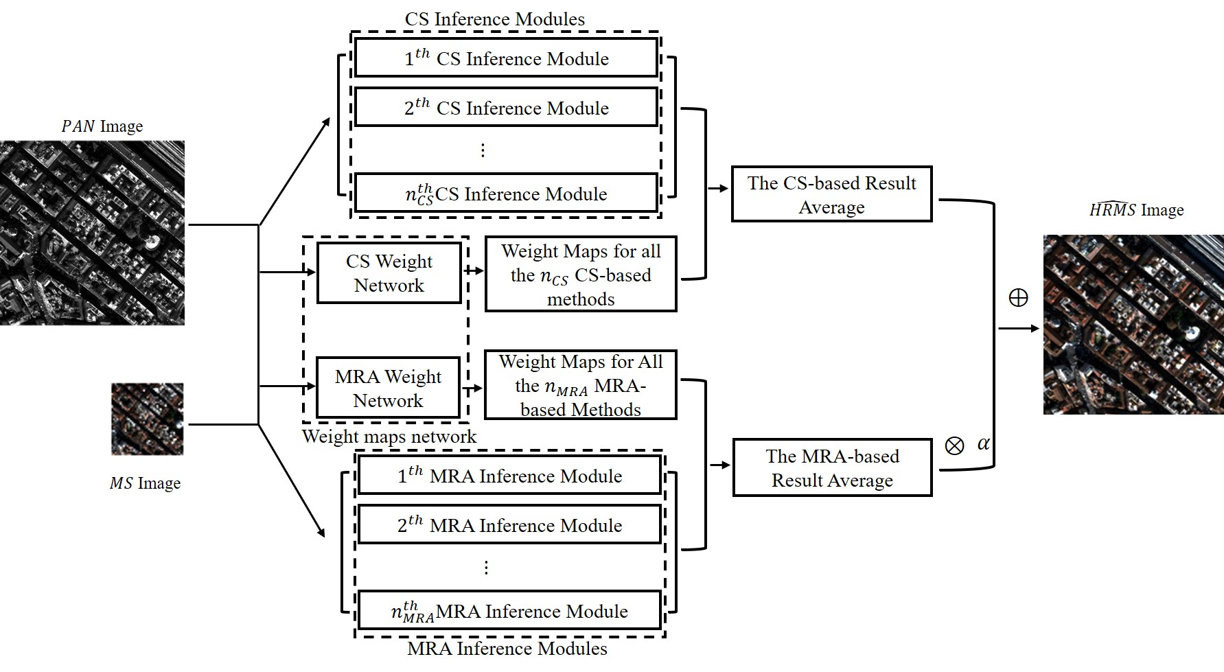
The CS-based methods are based on the assumption that the spatial and spectral information of LRMS image can be separated by a projection or transformation of the original LRMS image [3,37]. The CS class usually has four steps: (1) upsample the LRMS image to the size of the PAN image; (2) use a linear transformation to project the upsampled LRMS image into another space; (3) replace the component containing the spatial information with the PAN image; (4) perform an inverse transformation to bring the transformed MS data back to their original space and then get the pansharpened MS image (i.e., the estimated HRMS). Due to the changes in low spatial frequencies of the MS image, the substitution procedure usually suffers from spectral distortion. Thus, spectral matching procedure (i.e., histogram matching) is often applied before the substitution.
Mathematically, above fusion process can be simplified without the calculation of the forward and backward transformation as shown in Figure 1, which leads the CS class to have the following equivalent form as
where … are the injection gains, and is a linear combination of the upsampled LRMS image bands and often called intensity component, defined as
where … usually correspond to the first row of the forward transformation matrix, which is used to measure the degrees of spectral overlap between the MS and PAN channels.
Numerous CS-based methods have been proposed to sharpen the LRMS images according to Equation (1) and flowchart in Figure 1. The CS class includes IHS [9] which exploits the transformation into the IHS color space and its generalized version GIHS [10], PCA [11] based on the statistical irrelevance of each principal component, Brovey [12] based on a multiplicative injection scheme, Gram-Schmidt (GS) [13] which conducts the Gram-Schmidt orthogonalization procedure and by a weighted average of the MS bands minimizing the mean square error (MSE) with respect to a low-pass filtered version PAN image in the adaptive GS (GSA) [15], band-dependent spatial detail (BDSD) [14] and its enhanced version (i.e., BDSD with physical constraints: BDSD-PC) [16], partial replacement adaptive component substitute (PRACS) [17] based on the concept of partial replacement of the intensity component and so on. Each method differs from the others by the different projections of the MS images used in the process and by the different designs of injection gains. Although they show extreme performances in improving the spatial qualities of LRMS images, they usually suffer from heavily spectral distortions in some scenarios due to local dissimilarity or the not well-separated spatial structure with the spectral information. Refer to [3] for more detailed discussions about this.
2.2. The MRA-Based Methods
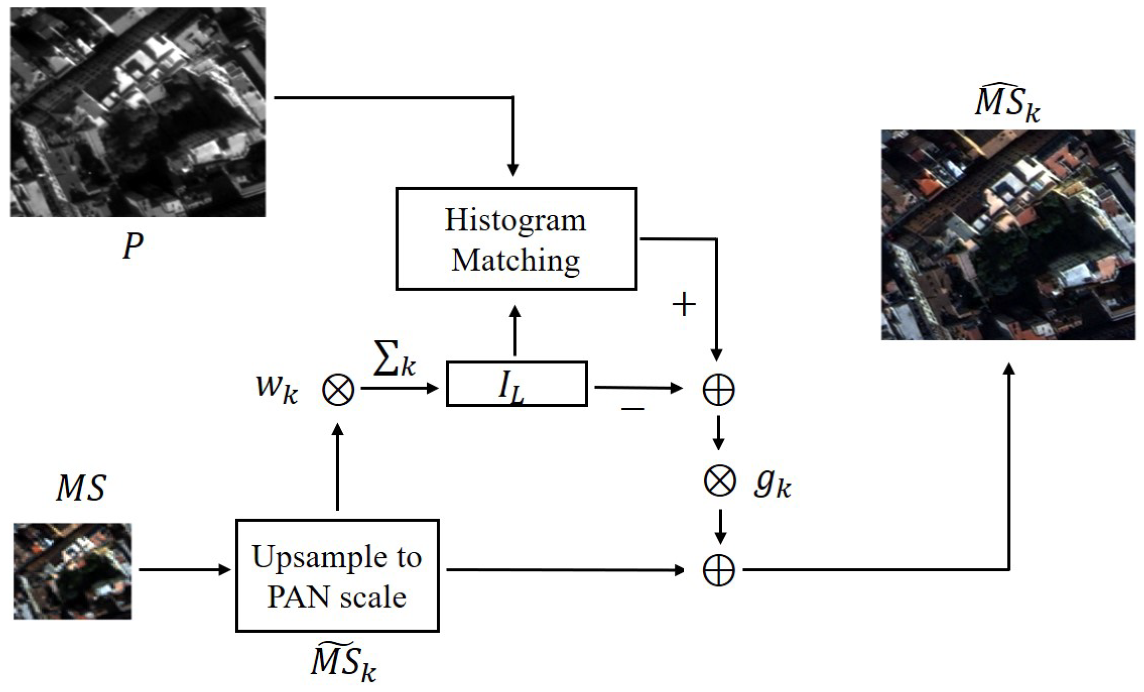
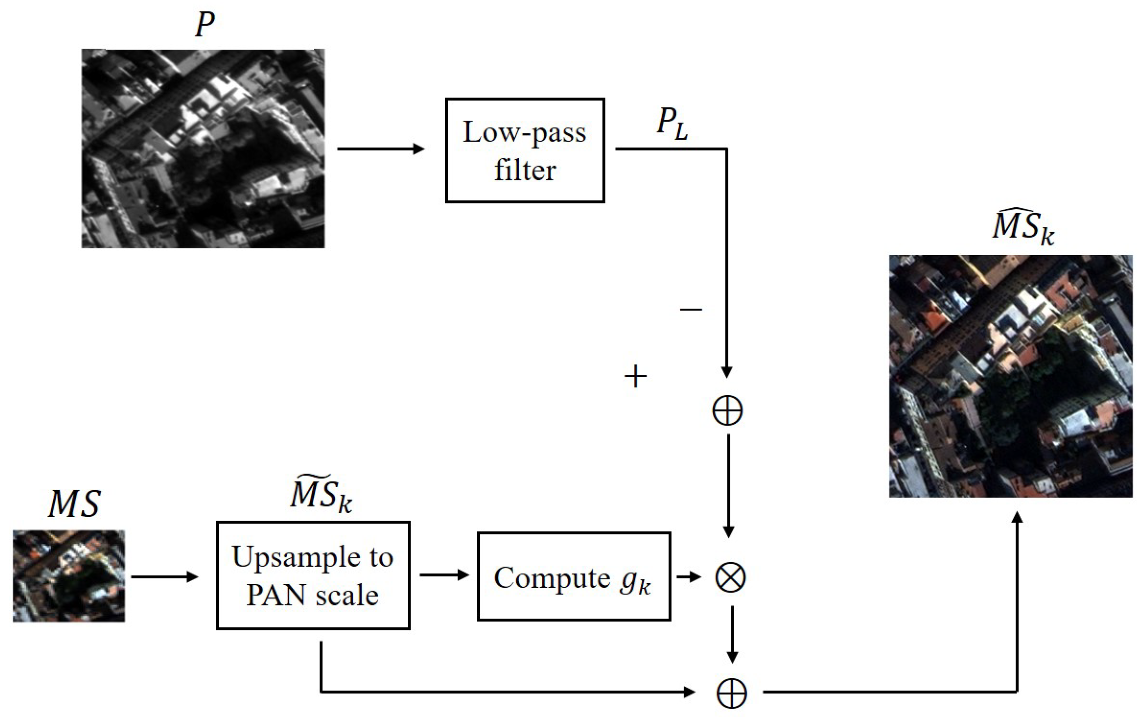
Unlike the CS-based methods, the MRA class is based on the operator of multi-scale decomposition or low-pass filter (equal to a single scale of decomposition) over the PAN image [3,37]. They first extract the spatial details over a wide range of scales from the high resolution PAN image or from the difference between the PAN image and its low-pass filtered version , and then inject the extracted spatial details into each band of upsampled LRMS image. Figure 2 shows the general flowchart of the MRA-based methods.
Generally, for each band , the MRA-based methods can be formulated as
As we can see from above Equation (3), different MRA-based methods can be distinguished by the way of obtaining and by the design of injection gains . Several methods belonging to this class have been proposed, such as HPF [18] using the box mask and additive injection, the SFIM [19], decimated Wavelet transform using additive injection model (Indusion) [23], the AWLP [24], GLP with modulation transfer function (MTF)-matched filter (denoted by MTF-GLP) [21], its HPM injection version (MTF-GLP-HPM) [22] and context-based decision version (MTF-GLP-CBD) [38], a trous wavelet transform using the model 3 (ATWT-TM3) [39], and so on.
The MRA-based methods highlight the extraction of multi-scale and local details from the PAN image, well in reducing the spectral distortion but compromising the spatial enhancement. To make up this problem, many approches have been proposed by the utilization of different decomposition schemes (e.g., morphological filters [40]) and the optimization of the injection gains.
2.3. The Learning-Based Method
Apart from the traditional CS-based and MRA-based methods, the learning-based methods have been proposed or applied to the pansharpening, among which the CNN-based methods are the most popular [41]. The CNN-based methods are very flexible, and one can design a CNN with different architectures. Due to the end-to-end and data-driven properties, they achieve the state-of-the-art performances in some studies [32,33,34,35]. After a network architecture design, training image pairs with low resolution MS (LRMS) images as network input and high resolution MS (HRMS) images as network output, are needed to learn the network parameters . The learning procedure is based on the choice of loss function and optimization method, and the effect of learning is different from each other according to these choices of loss function and optimization strategy. However, these ideal image pairs are unavailable, and usually simulated based on scale invariant assumption by properly downsampling both PAN and the original MS images to a reduced resolution. Then, the resolution reduced MS images and the original MS can be used as an input-output pair.
Given the input-output MS pairs of with low resolution and with high resolution, and aided by the auxiliary PAN image , …, the CNN-based methods optimize the parameter by minimizing the following cost function
where denotes a neural network which takes as parameters, and is the Frobenius norm, which is defined as the square root of the sum of the absolute squares of the elements.
To further improve the performances of CNN-based methods, recent work mainly resorts to the deep residual architecture [42] or to increase the depth of the model to extract multi-level abstract features [43]. However, these will require large number of network parameters and burden computation [36]. Unlike the above CNN-based methods that aim at generating the HRMS images or their residual images, we here to reduce the number of parameters and reduce the requirements on the computation capacity of the computer by learning weight maps for the CS-based and the MRA-based methods. Refer to the following section for more detailed discussions about this.
3. The Proposed PWNet Method
3.1. Motivation and Main Idea
According to the above analysis, the CS-based and MRA-based methods are simple and usually have complementary performances, i.e., the CS-based methods are good at spatial rendering but sometimes suffer from severe spectral distortions, while the MRA-based methods performance well in keeping the spectral information of the MS images but may have limited spatial enhancements. And the performances of the CS-based and MRA-based methods show data uncertainty, i.e., they have different fusion performances on different scenarios. The learning-based methods, especially the CNN-based methods, perform well in reducing spatial and spectral distortions due to their powerful feature extraction capabilities and data-driven training scheme. However, they usually need an extremely large data set to train the model parameters and are difficult to be interpretable.
Is there a way to make full use of the complementary performances of the CS-based and MRA-based methods at the same time reducing their data uncertainty? A straightforward idea is to firstly generate multiple fusion results by multiple methods (i.e., the CS-based and MRA-based methods), and then automatically combine them with weights based on performances within different scenarios to boost the fusion result. This may be realized by using a trainable CNN since it is data-driven and has strong abilities in the field of image processing.
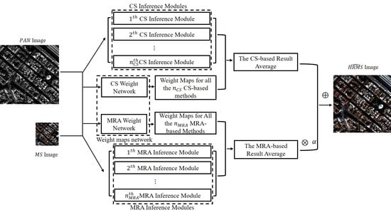
Motivated by the above, we propose a novel model average method, referred to as pansharpening weight netowrk (PWNet), for the pansharpening. Specifically, rather than generating only one estimated HRMS image at a time, we use multiple inference modules to generate distinct estimated HRMS images at a time. Each inference module produces a distinct estimate of HRMS with bias, and multiple estimates have the positive and negative deviations. And then the biases can be complemented by averaging the multiple results, thus leading to the distortions of average are smaller than that of a single estimate. In order to make use of the simplicity and complementary characteristics of the CS-based and MRA-based methods, we choose them as inference modules, i.e., use each CS-based or MRA-based method as an inference module, and then design an end-to-end trainable network with the original MS and PAN images as input to simultaneously obtain weight maps for all fusion results obtained by the CS and MRA inference modules. Based on the powerful capability and data-driven training scheme of nerual network, the output weight maps are context and method dependent. Finally, we get an estimated HRMS image through adaptively averaging all the fusion results obtained by the CS-based and MRA-based methods. Figure 3 depicts the main procedures of the proposed PWNet for pansharpening.
3.2. Network Architecture
Pansharpening Weight Network (PWNet): The key of model average is to assign proper weights to different models depending on their performances. Unlike traditional model average methods that are based on hand-crafted design to assign weights, we resort the neural network to adaptively generate weights. The proposed PWNet is composed of two subnet: the CS weight network and the MRA weight network. For each subnet, the original LRMS and/or PAN images are took as input. Similar to [33], high-pass filter operation is first implemented in order to preserve edges and details. For the CS weight subnet, the high-pass filtered MS image is upsampled though a transpose convolution and concatenated with the high-pass filtered PAN image, and then fed into four residual blocks [44]. Different from this, the MRA weight subnet only passes the high-pass filtered PAN image into the subsequent residual blocks. Each of the residual blocks consists of three convolutional layers with each having a learnable filter of size and a rectified-linear unite (ReLU) activation function [45]. To generate weight maps, the activation function of the output layer is set to be a softmax function. By considering computation efficiency and also for keeping the proportions between each pair of the MS bands unchanged, the PWNet only outputs one weigh map for each CS-based or MRA-based method to achieve a pixel-wise aggregation, which will be discussed below. The detailed architecture of PWNet for generating the weight maps is shown in Figure 4.
The CS-based Result Average: Suppose we have kinds of CS-based methods for our PWNet, and then, for the ith CS-based method, we have its estimated HRMS image as
where , is the kth MS band and denotes the ith CS-based method. According to the CS weight network, we get adaptive weight maps for the used CS-based methods as:
where is the ith output weight map generated by the CS weight network, denotes the CS weight network, is the parameter set, the function is the high-pass filter. At last, we conduct pixel-wise multiplication for each estimated HRMS image and its corresponding weight map and sum the multiplication results to get the CS-based result average, i.e., for each band, we have the averaged result as
where denotes the result of the kth band of CS-based method module and ⊙ denotes the point-wise multiplication.
The MRA-based Result Average: Consistent with the procedures of the CS-based method module, the averaged results for the MRA-based methods can be given as
where and are the kth HRMS band obtained by the ith MRA-based method and the ith output weight map generated by the MRA weight network, which respectively are given as
and
where denotes the MRA weight network, is the parameter set, and is the ith MRA-based method. Note that, different from the CS-based weight network, we only take the PAN image as the input of the MRA-based weight network since the MRA-base methods extract the spatial details only rely on the PAN image.
The Final Result Aggregation: After we have obtained the averaged results of the CS-based method module, , and the averaged results of the MRA-based method module, , then we can aggregate them for compensating their spatial and/or spectral distortions. The final estimated HRMS image can be given as
where is a factor for balancing the contributions between the CS-based methods and the MRA-based methods.
The Loss function: To learn the model parameters , we would like to minimize the reconstruction errors between the estimated HRMS image, , and its corresponding ideal one, Y, i.e.,
where n is the number of training samples.
4. Experiments
4.1. Data Sets and Implementation Details
We conduct several experiments using three data sets respectively collected by the GeoEye-1, WorldView-2, and QuickBird satellites. Each data set is split into two nonoverlapping subset: a training data set and a testing data set. Each sample in the data set consists of an MS and PAN image pairs with the PAN image of size and the MS image of size . In order to verify the generalization of the proposed method, we also perform pansharpening on a scene taken on other days for QuickBird satellite at the full resolution experiment. More detailed information of the three data sets is reported in Table 1.
As for the training of our proposed PWNet, due to the unavailable of the ideal HRMS images, similar to the other CNN-based pansharpening methods [32,33,34], we first follow the Wald’s protocol [46] to generate the training input MS and PAN pairs by downsampling both the original PAN and MS images with scale factor (i.e., the resolution of the MS and PAN images is reduced by applying the MTF-matched low-pass filters [21]), and then the the original MS images are treated as target outputs.
The PWNet is implemented in Tensorflow and trained on a Intel(R) Core(TM) i5-4210U CPU. We use the Adam algorithm [47] with an initial learning rate of 0.001 to optimize the network parameters. And we set the maximum number of epoch to 1000 and mini-batch sample size to 32. It takes about 1 h to train our network.
We first evaluate the methods at a reduced resolution, in addition to visual analysis on the experimental results, the proposed PWNet and other compared methods are also evaluated by five widely used quantitative metrics, namely, universal image quality index [48] averaged over the bands (Q_avg) and its four band extension, Q4 [3], spectral angle mapper (SAM) [49], Erreur Relative Globale Adimensionnelle de Synthse (ERAGS) [50] and the spatial correlation coefficient (SCC) [46]. The closer to one the Q_avg, Q4, and SCC, the better the quality of fused results, while the lower the SAM and ERGAS, the better the fusion quality.
We also evaluate the methods at a full resolution. In this case, the quality with no-reference index (QNR) [51] and its spatial index () and spectral index () are employed for the quantitative assessment. It should be pointed out that the quantitative assessment at full resolution is challenging since these indexes (i.e., QNR, and ) are not computed with unattainable ground truth, but rely heavily on the original MS and PAN images [43]. This tends to quantify the similarity of certain components in the fused images to the low-resolution observations, which will lead biases in these indexes estimation. Due to this reason, some methods can generate images with high QNR values but poor image qualities [52].
In the following, we have carried out five sets of experiments to perform comprehensive analysis on the proposed PWNet, typically the effect of the hyperparameter , the number of CS-based and MRA-based methods, the weight maps channels, and the quantitative, visual and running time comparisons with the CS-based, MRA-based and learning-based methods at reduced resolution and full resolution.
4.2. Analysis to the Hyper-Parameters
There is a hyper-parameter in our proposed PWNet, which is to balance the contributions of the CS-based and MRA-based methods. In this experiment, we will analyze this parameter to optimize the performance of PWNet. We fix the number of CS-based and MRA-based methods to six and change from 0.1 to 1 with interval 0.1. The results obtained are shown in Table 2. As we can see from it, the PWNet attains constantly good performances when varies from 0.7 to 0.9. Specially, the best results can be obtained for . It is worth noting that when goes to 1, the quantitative indexes seem to become worse. Thus, can be a relatively good choice in the following experiments.
4.3. Impact of the Number of the CS-Based and MRA-Based Methods
This experiment shows what influences would be produced by the different number of the CS-based and MRA-based methods under the condition of for simplicity and also for keeping the balance between the CS class and the MRA class methods. The number of methods to be averaged is very important to balance the spectral and spatial information from the LRMS and high resolution PAN images. Too few methods might extract features incompletely and result in a poor performance, while too many would suffer from computational burden during testing. We would like to find a trade-off value according to the performance and running time. Therefore, we limit the range of (or ) to between 5 and 8.
Table 3 gives the quantitative results and the running time (in second) when the number of averaged methods varies from 5 to 8. Note that, and equal 5, which means that the selected CS-based are PCA [11], GIHS [10], Brovey [12], GS [13], GSA [15] and the selected MRA-based methods are HPF [18], SFIM [19], AWLP [24], MTF-GLP-HPM [22], MTF-GLP-CBD [38], respectively. When both and are equal to 6, the PRACS [17] and the ATWT-M3 [39] methods are added into the CS-based and MRA-based methods, respectively. When and are equal to 7, we add the BDSD [14] into the CS weight network and the Indusion [23] into the MRA weight network, and the BDSD-PC [16] and the MTF-GLP [21] are added into the CS weight network and the MRA weight network as method modules when and are equal to 8. As reported in Table 3, the performance of the proposed PWNet is improved when the number of averaged methods increases from 5 to 7, while it decays when and are equal to 8. This reveals that the use of less number of averaged methods will reduce the performances of the PWNet and increasing the number of averaged methods will not continuously bring improvements but will suffer from more computation. In principle, our proposed PWNet is data-driven and thus can automatically weight different kinds of CS-based and/or MRA-based methods. In practice, we suggest two criteria for the selection of CS-based and MRA-based methods for the proposed PWNet. First, the number of CS-based methods and the number of MRA-based methods should be equal in order to keep the balance contribution of the CS class and MRA class. And then, to further improve the performances and robustness of the PWNet, we suggest selecting the CS-based and MRA-based methods according to their performances reported in [3].
4.4. Impact on the Number of Weight Map Channels
In order to reduce the number of parameters and the computational cost, we set the weight map for each CS-based or MRA-based method to be one channel. That is, each MS band of a HRMS image obtained by a CS-based or MRA-based method share the same weight map. In general, the model capacity will be increased with the number of model parameters. Thus, we conduct the experiments based on different output weight map channels to verify whether the capacity of our model has suffered from the reduction of channels.
The results of PWNet with one shared weight map channel and with four different weight map channels for each CS-based or MRA-based method are reported in Table 4. As we can see from it, the PWNet with one shared weight map channel attains constantly good performances in terms of the five commonly used metrics on three different kinds of satellite data sets, while the PWNet with four different weight map channels for each method has a relatively poor performances with the same training conditions. This may due to that an under-fitting phenomenon caused by excessive parameters has happened in the PWNet with four weight map channels. It further verifies the advantages of the PWNet with one shared weight map channel, which can lower the training difficulty.
4.5. Comparison with the CS-Based and MRA-Based Methods
One key issue of the proposed PWNet method is whether its fusion result is better than that of each participating method. Only when the answer to this question is yes, we can claim that the proposed PWNet can produce appropriate weight maps for each CS-based or MRA-based method, so that the methods involved in model average can complement each other and the result can be improved. Here we set and to 7 as we have proved in above that this setting has a good balance for performances and running times. The compared pansharpening methods include seven methods belonging to the CS class, namely, PCA [11], GIHS [10], Brovey [12], BDSD [14], GS [13], GSA [15], PRACS [17], and seven methods belonging to the MRA class such as HPF [18], SFIM [19], Indusion [23], AWLP [24], ATWT-M3 [39], MTF-GLP-HPM [22], MTF-GLP-CBD [38]. All methods follow the experimental settings recommended by the authors.
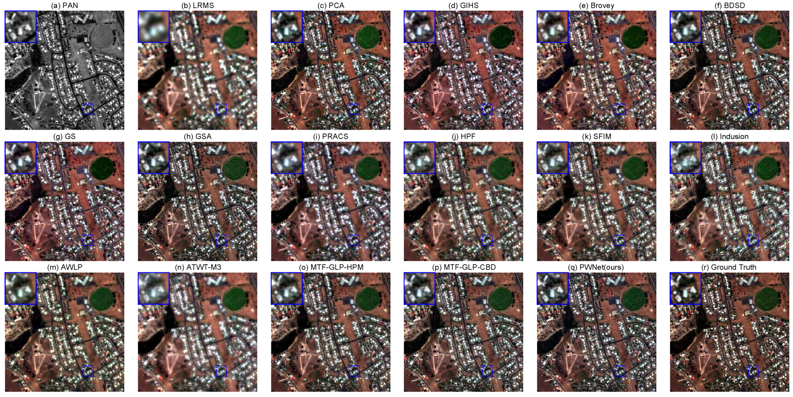
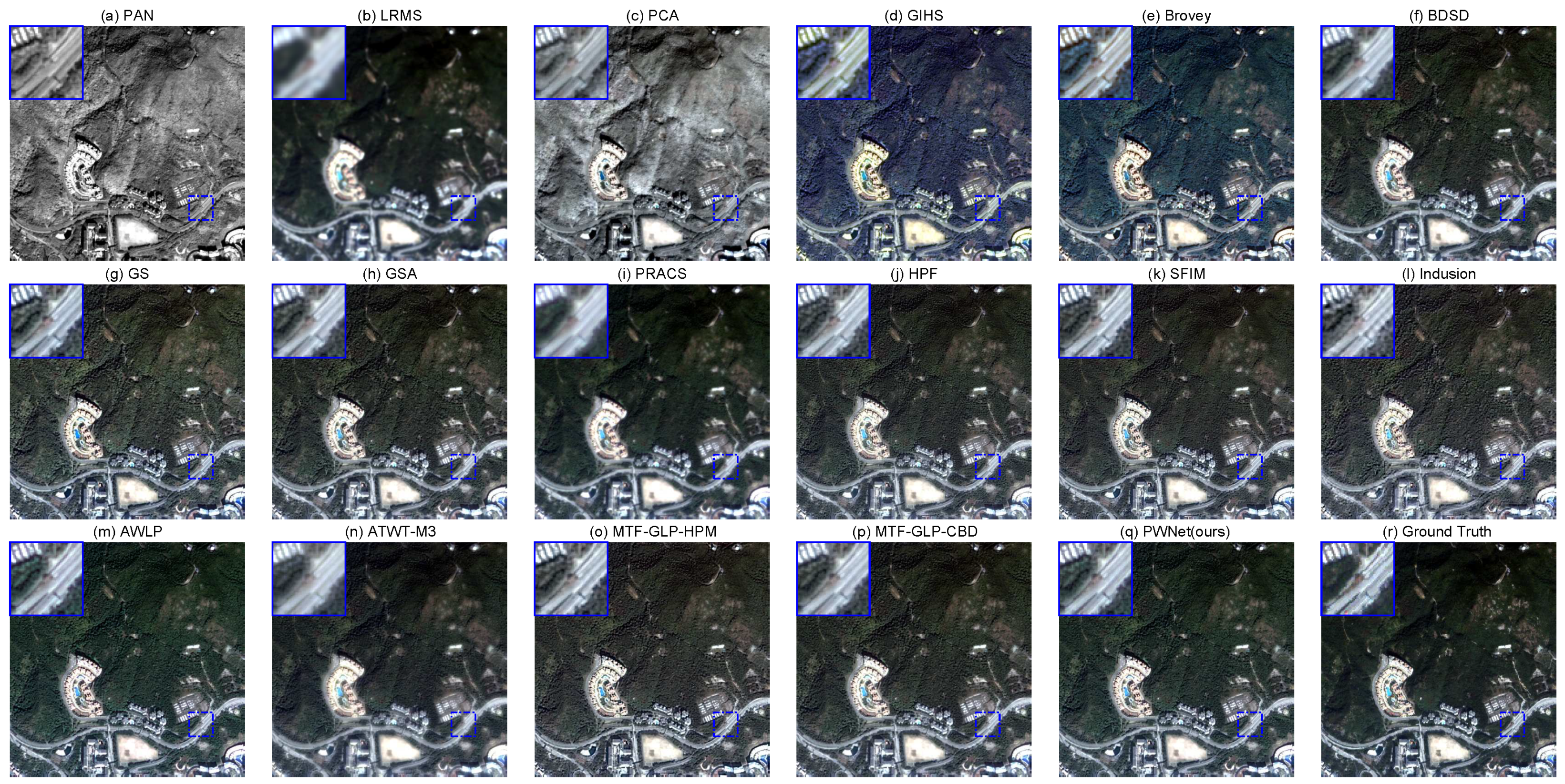
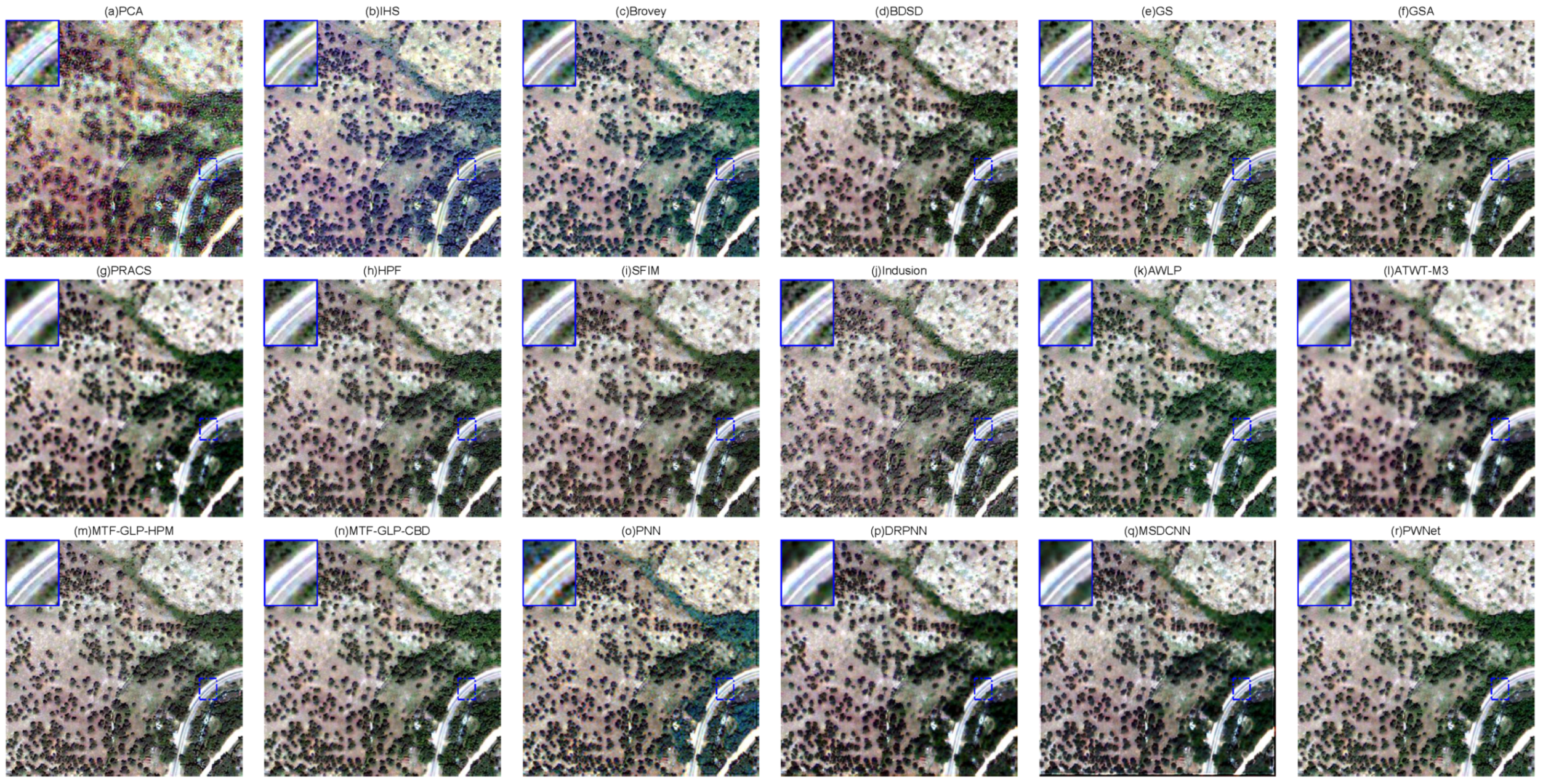
We first inspect the visual quality of the pansharpening results. Figure 5, Figure 6 and Figure 7 present the pansharpened images on all the three data sets, obtained by our proposed PWNet and the other fourteen methods. As we can see from theses figures, the CS-based methods produce a relatively sharper spatial features in Figure 5a–g, but they suffer from spectral distortions, as highlighted in the small window, where the trees around buildings in Figure 5 and the bare soil in Figure 6 are a little darker than that of ground truth. In contrast, less spectral distortions are appeared in the results of the MRA-based methods, however, they show poor spatial rendering as they present a little blurring in Figure 6h–n, especially for the results of AWLP and ATWT-M3. Compared with the CS-based and MRA-based methods, the proposed PWNet can achieve more similar results to the ground truth. From the enlarged area in the upper left corner of the Figure 7o, we can see that PWNet has the best performance in both improving the spatial details and keeping spectral fidelity of the roads and trees. In summary of the visual analysis, the proposed PWNet method can debias the spectral and spatial distortions in the CS-based and the MRA-based methods, and can effectively combine the advantages of these two types of methods, thus shows better visual performances.
Besides visual inspection, we apply numeric metrics to assess the quality of pansharpened images. Table 5, Table 6 and Table 7 report the comparison results of the CS-based methods, MRA-based methods, and the proposed PWNet method on the three data sets. As we can find from these tables, for the WordView-2 and GeoEye-1 data sets, the BDSD method shows the best performances among the fourteen traditional methods, the AWLP achieves the best performance among the CS-based and MRA-based methods for the QuickBird data set. None of the CS-based and MRA-based methods systematically obtain the best performances for all the three data sets. The proposed PWNet yields results with the best spatial and spectral accuracy over the CS-based and MRA-based methods on all the three data sets. This proves once again that the proposed method can combine the advantages of the two types of methods to produce an optimal result.
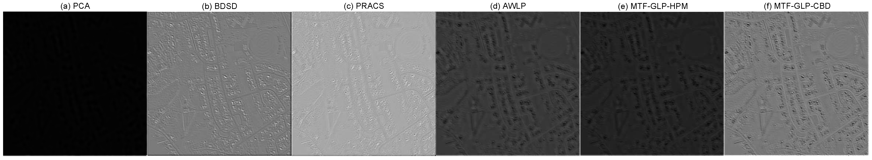
To be interpretable, we also visualize the some weight maps of the selected traditional methods used in the PWNet, as shown in Figure 8, Figure 9 and Figure 10. It can be seen from these figures that, the edges of the road and the buildings are extracted by the weight maps of both the CS-based and MRA-based methods. Typically, we can see that, for the WorldView-2 and GeoEye-1 data sets, the BDSD method plays an important role as its weight map is clearer than any others, as showin in Figure 8b and Figure 9b, while the AWLP and MTF-GLP-CBD methods show a little greater contribution to the averaged results of the PWNet for the QuickBird data set, as can be see from Figure 10d,e. As for the PCA method, the weight maps are all black, which means that PCA method almost makes no contribution to the final result on all the three tested data sets. This conclusion is consistent with the previous visual inspection in Figure 5, Figure 6 and Figure 7 and quantitative results reported in Table 5, Table 6 and Table 7. This proves the adaptive characteristic of our PWNet as it considers different performance of the selected CS-based and MRA-based methods. From these experimental results, we can conclude that the proposed PWNet are adaptive and robust to different data sets.
4.6. Comparison with the CNN-Based Methods
Currently, the proposed PWNet has shown its priority over the selected traditional CS-based and MRA-based methods. In this subsection, we are going to compare it with the CNN-based methods to verify its effectiveness. The other four stat-of-the-art (SOTA) methods including pansharpening by convolutional neural networks (PNN) [32], deep residual pan-sharpening neural network (DRPNN) [42], multiscale and multidepth convolutional neural network (MSDCNN) [43], are used as alternative methods for comparison. All the compared methods follow the experimental setting of their original papers. Note that the source codes of PNN is provided by the original authors and the codes of DRPNN, MSDCNN are available at https://github.com/Decri.
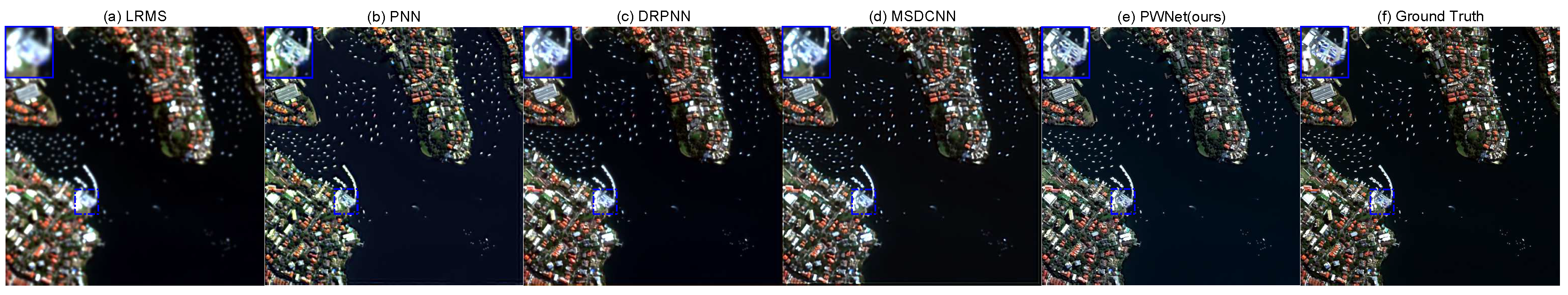
Figure 11, Figure 12 and Figure 13 show some example regions selected from the pansharpened images on the three test data sets. In Figure 11, by magnifying the selected area in the image three times, it can be obviously seen that the other CNN-based methods have a little blurring to the ground truth, while the edges produced by our proposed PWNet method are more clear and natural as shown in zoomed areas. Although MSDCNN, DRPNN and PNN can produce better results with less spatial distortions, they sometimes suffer from a little spectral distortions, as shown in Figure 12b–d, where the bare soil is a little darker than the reference. This can also be seen in Figure 13b where the buildings in this scene is dark yellow while they are white in the ground truth as shown in Figure 13f. Compared with other CNN-based methods, the proposed PWNet shows a good balance between the injected spatial details and the maintain of original spectral information, this is clearly visible on the vegetable areas and textures (e.g., edges of the roof and road), as shown in Figure 11e, Figure 12e and Figure 13e.
In addition, Table 8 shows the quantitative results for the three tested data sets obtained by the compared CNN-based methods and our proposed PWNet. It should be pointed out that, for each test experiment, we would choose one test sample randomly from the test data set rather than a cherry-picked sample, thus the results listed in Table 8 and Table 5, Table 6 and Table 7 are based on different PAN and MS image pairs and have different quantitative results. For better comparison, the best results among the four methods are highlighted in boldface. According to this table, one can see that performances of the proposed PWNet is better than the other three CNN-based methods in terms of the five indexes.
4.7. Comparison at Full Resolution
The comparison results on three tested images at full resolution are shown in Figure 14, Figure 15 and Figure 16 and Table 9. As we can see from the table that, for the WordView-2 and GeoEye-1 data sets, the DRPNN and PNN method respectively show the best performances, while the proposed PWNet holds the second best position for all the three data sets. On a whole, the CNN-based methods perform better than the traditional methods (i.e., the CS-based and MRA-based methods). By a visual inspection, the PNN, DRPNN, and MSDCNN methods tend to produce blurring results while the proposed PWNet is able to enhancing the spatial quality and shows clearly sharper fusion results, as shown in Figure 14, Figure 15 and Figure 16r. As a summary, compared to the other methods at the full resolution, the proposed PWNet could consistently reconstruct sharper HRMS image with less spectral and spatial distortion.
4.8. Running Time Analysis
In this subsection, we compare the running time of the proposed method with the others on a LRMS and PAN image pair. The experiments are performed by MATLAB R2016b on the same platform with Core i5-4210U/1.7 GHz/4G. The running times of different methods are listed in Table 10, in which the time is measured in second. From this table, it can be found that DRPNN is the most time-consuming method, because the number of hidden layers within DRPNN is more than the other CNN-based methods. In addition, the MSDCNN needs a little more time to obtain the fusion result than that of the proposed PWNet. In a word, the proposed PWNet method is more efficient than the CNN-based methods due to less hidden layers and that it only outputs weight maps rather than directly producing an estimated HRMS image.
5. Conclusions
In this paper, we presented a novel model average network for pansharpening, and is referred to as PWNet. The proposed PWNet attempts to integrate the complementary characteristics of the CS-based and MRA-based methods through an end-to-end trainable neural networks, and thus it is data-driven and able to adaptively weight the results of the classical methods depending on their performances. Experiments on several data sets collected by three kinds of satellites demonstrate that the pansharpened HRMS images by the proposed PWNet can not only enhance the spatial qualities but also can keep the spectral information of the original MS images. In addition, the proposed PWNet has some distribution structures. Thus, we will extend the proposed model to a distribution version by using the techniques of distributed processing [53] to further reduce the running time while maintaining the quality of the results.
Author Contributions
J.L. and C.Z. (Chunxia Zhang) structured and drafted the manuscript with assistance from C.Z. (Changsheng Zhou); Y.F. conceived the experiments and generated the graphics with assistance from C.Z. (Changsheng Zhou). All authors have read and agreed to the published version of the manuscript.
Funding
This research was funded by the National Key Research and Development Program of China under Grant 2018AAA0102201, and by the National Natural Science Foundation of China grant number 61877049.
Acknowledgments
Conflicts of Interest
The authors declare no conflict of interest.
References
- Shaw, G.; Burke, H.K. Spectral imaging for remote sensing. Linc. Lab. J. 2003, 14, 3–28. [Google Scholar]
- Meng, X.; Shen, H.; Li, H.; Zhang, L.; Fu, R. Review of the pansharpening methods for remote sensing images based on the idea of meta-analysis: Practical discussion and challenges. Inf. Fusion 2019, 46, 102–113. [Google Scholar] [CrossRef]
- Vivone, G.; Alparone, L.; Chanussot, J.; Dalla Mura, M.; Garzelli, A.; Licciardi, G.A.; Restaino, R.; Wald, L. A critical comparison among pansharpenig algorithms. IEEE Trans. Geosci. Remote Sens. 2015, 53, 2565–2586. [Google Scholar] [CrossRef]
- Ehlers, M.; Klonus, S.; Astrand, P.; Rosso, P. Multi-sensor image fusion for pansharpening in remote sensing. Int. J. Image Data Fusion 2010, 1, 25–45. [Google Scholar] [CrossRef]
- Yue, L.; Shen, H.; Li, J.; Yuan, Q.; Zhang, H.; Zhang, L. Image super-resolution: The techniques, applications, and future. Signal Process. 2016, 128, 389–408. [Google Scholar] [CrossRef]
- Souza, C.; Firestone, L.; Silva, M.; Roberts, D. Mapping forest degradation in the Eastern Amazon from SPOT 4 through spectral mixture models. Remote Sens. Environ. 2003, 87, 494–506. [Google Scholar] [CrossRef]
- Mohammadzadeh, A.; Tavakoli, A.; Valadan Zoej, M.J. Synthesis of multispectral images to high spatial resolution: Road extraction based on fuzzy logic and mathematical morphology from pansharpened IKONOS images. Photogramm. Rec. 2006, 21, 44–60. [Google Scholar] [CrossRef]
- Loncan, L.; De Almeida, L.B.; Bioucas-Dias, J.M.; Briottet, X.; Chanussot, J.; Dobigeon, N.; Fabre, S.; Liao, W.; Licciardi, G.A.; Simoes, M.; et al. Hyperspectral pansharpening: A review. IEEE Geosci. Remote Sens. Mag. 2015, 3, 27–46. [Google Scholar] [CrossRef] [Green Version]
- Carper, W.; Lillesand, T.; Kiefer, R. Synthesis of multispectral images to high spatial resolution: The use of intensity-huesaturation transformations for merging SPOT panchromatic and multispectral image data. Photogramm. Eng. Remote Sens. 1990, 56, 459–467. [Google Scholar]
- Tu, T.; Su, S.C.; Shyu, H.C.; Huang, P.S. A new look at IHS-like image fusion methods. Inf. Fusion 2001, 2, 177–186. [Google Scholar] [CrossRef]
- Chavez, P.S.; Kwarteng, A.W. Extracting spectral contrast in Landsat thematic mapper image data using selective principal component analysis. Photogramm. Eng. Remote Sens. 1989, 55, 339–348. [Google Scholar]
- Gillespie, A.; Kahle, A.B.; Walker, R.E. Color enhancement of highly correlated images-II. Channel ration and “Chromaticity” Transform techniques. Remote Sens. Environ. 1987, 22, 343–365. [Google Scholar] [CrossRef]
- Laben, C.A.; Brower, B.V. Process for Enhancing the Spatial Resolution of Multispectral Imagery Using Pan-Sharpening. U.S. Patent 6011875, 4 January 2000. [Google Scholar]
- Garzelli, A.; Nencini, F.; Capobianco, L. Optimal MMSE pan sharpening of very high resolution multispectral images. IEEE Trans. Geosci. Remote Sens. 2008, 46, 228–236. [Google Scholar] [CrossRef]
- Aiazzi, B.; Baronti, S.; Selva, M. Improving component substitution pansharpening through multivariate regression of MS+Pan data. IEEE Trans. Geosci. Remote Sens. 2007, 45, 3230–3239. [Google Scholar] [CrossRef]
- Vivone, G. Robust band-dependent spatial-detail approaches for panchromatic sharpening. IEEE Trans. Geosci. Remote Sens. 2019, 57, 6421–6433. [Google Scholar] [CrossRef]
- Choi, J.; Yu, K.; Kim, Y. Synthesis of multispectral images to high spatial resolution: A new adaptive component-substitution based satellite image fusion by using partial replacement. IEEE Trans. Geosci. Remote Sens. 2011, 49, 295–309. [Google Scholar] [CrossRef]
- Chavez, P.S., Jr.; Sides, S.C.; Anderson, A. Comparison of three different methods to merge multiresolution and multispectral data: Landsat TM and SPOT panchromatic. Photogramm. Eng. Remote Sens. 1991, 57, 295–303. [Google Scholar]
- Liu, J. Smoothing filter-based intensity modulation: A spectral preserve image fusion technique for improving spatial details. Int. J. Remote Sens. 2000, 21, 3461–3472. [Google Scholar] [CrossRef]
- Aiazzi, B.; Alparone, L.; Baronti, S.; Garzelli, A.; Selva, M. An MTF based spectral distortion minimizing model for pan-sharpening of very high resolution multispectral images of urban areas. In Proceedings of the 2nd GRSS/ ISPRS Joint Workshop Remote Sensing and Data Fusion URBAN Areas, Berlin, Germany, 22–23 May 2003; pp. 90–94. [Google Scholar]
- Aiazzi, B.; Alparone, L.; Baronti, S.; Garzelli, A.; Selva, M. MTF tailored multiscale fusion of high-resolution MS and Pan imagery. Photogramm. Eng. Remote Sens. 2006, 72, 591–596. [Google Scholar] [CrossRef]
- Vivone, G.; Restaino, R.; Dalla Mura, M.; Licciardi, G.; Chanussot, J. Contrast and error-based fusion schemes for multispectral image pansharpening. IIEEE Trans. Geosci. Remote Sens. 2014, 11, 930–934. [Google Scholar] [CrossRef] [Green Version]
- Khan, M.M.; Chanussot, J.; Condat, L.; Montavert, A. Indusion: Fusion of multispectral and panchromatic images using the induction scaling technique. IEEE Trans. Geosci. Remote Sens. 2008, 5, 98–102. [Google Scholar] [CrossRef] [Green Version]
- Otazu, X.; González-Audìcana, M.; Fors, O.; Núñez, J. Introduction of sensor spectral response into image fusion methods. Application to wavelet-based methods. IEEE Trans. Geosci. Remote Sens. 2005, 43, 2376–2385. [Google Scholar] [CrossRef] [Green Version]
- Shah, V.P.; Younan, N.H.; King, R.L. An efficient pan-sharpening method via a combined adaptive PCA approach and contourlets. IEEE Trans. Geosci. Remote Sens. 2008, 46, 1323–1335. [Google Scholar] [CrossRef]
- Liao, W.; Huang, X.; Van Coillie, F.; Gautama, S.; Pižurica, A.; Philips, W.; Liu, H.; Zhu, T.; Shimoni, M.; Moser, G.; et al. Processing of Multiresolution Thermal Hyperspectral and Digital Color Data: Outcome of the 2014 IEEE GRSS Data Fusion Contest. IEEE J. Sel. Top. Appl. Earth Observ. Remote Sens. 2015, 8, 2984–2996. [Google Scholar] [CrossRef]
- Ballester, C.; Vselles, V.; Igual, L.; Verdera, J.; Rouge, B. A variational model for P+XS image fusion. Int. J. Comput. Vis. 2006, 69, 43–58. [Google Scholar]
- Moller, M.; Wittman, T.; Bertozzi, A.; Berger, M. A variational approach for sharpening high dimensional images. SIAM J. Imaging Sci. 2012, 5, 150–178. [Google Scholar] [CrossRef] [Green Version]
- Zhu, X.; Bamler, R. A sparse image fusion algorithm with application to pansharpening. IEEE Trans. Geosci. Remote Sens. 2013, 51, 2827–2836. [Google Scholar] [CrossRef]
- Deng, L.; Vivone, G.; Guo, W.; Mura, M.; Chanussot, J. A variational pansharpening approach based on reproducible kernel hilbert space and heaviside function. IEEE Trans. Image Process. 2018, 27, 4330–4344. [Google Scholar] [CrossRef]
- Palsson, F.; Ulfarsson, M.; Sveinsson, J. Model-based reduced-rank pansharpening. IEEE Geosci. Remote Sens. Lett. 2020, 17, 656–660. [Google Scholar] [CrossRef]
- Masi, G.; Cozzolino, D.; Verdoliva, L.; Scarpa, G. Pansharpening by convolutional neural networks. Remote Sens. 2016, 8, 594. [Google Scholar] [CrossRef] [Green Version]
- Yang, J.; Fu, X.; Huang, Y.; Ding, X.; Paisley, J. PanNet: A deep network architecture for pan-sharpening. In Proceedings of the International Conference on Computer Vision, Venice, Italy, 22–29 October 2017; pp. 5449–5457. [Google Scholar]
- Liu, X.; Wang, Y.; Liu, Q. Synthesis of multispectral images to high spatial resolution: Remote sensing image fusion based on two-stream fusion network. IEEE Trans. Geosci. Remote Sens. 2018, 46, 428–439. [Google Scholar]
- Zheng, Y.; Li, J.; Li, Y.; Guo, J.; Wu, X.; Chanussot, J. Hyperspectral Pansharpening Using Deep Prior and Dual Attention Residual Network. IEEE Trans. Geosci. Remote Sens. 2020, 10, 1–18. [Google Scholar] [CrossRef]
- Han, S.; Pool, J.; Tran, J.; Dally, W. Learning both weights and connections for efficient neural network. In Proceedings of the Advances in Neural Information Processing Systems 2015, Montreal, QC, Canada, 7–12 December 2015; pp. 1135–1143. [Google Scholar]
- Ghamisi, P.; Rasti, B.; Yokoya, N.; Wang, Q.; Hofle, B.; Bruzzone, L.; Bovolo, F.; Chi, M.; Anders, K.; Gloaguen, R.; et al. Multisource and multitemporal data fusion in remote sensing: A comprehensive review of the state of the art. IEEE Geosci. Remote Sens. Mag. 2019, 7, 6–39. [Google Scholar] [CrossRef] [Green Version]
- Alparone, L.; Wald, L.; Chanussot, J.; Thomas, C.; Gamba, P.; Bruce, L. Comparison of pansharpening algorithms: Outcome of the 2006 GRS-S DataFusion Contest. IEEE Trans. Geosci. Remote Sens. 2007, 45, 3012–3021. [Google Scholar] [CrossRef] [Green Version]
- Ranchin, T.; Wald, L. Fusion of high spatial and spectral resolution images: The ARSIS concept and its implementation. Photogramm. Eng. Remote Sens. 2000, 66, 49–61. [Google Scholar]
- Restaino, R.; Vivone, G.; Dalla Mura, M.; Chanussot, J. Fusion of multispectral and panchromatic images based on morphological operators. IEEE Trans. Image Process. 2016, 25, 2882–2895. [Google Scholar] [CrossRef] [Green Version]
- Zhong, J.; Yang, B.; Huang, G. Remote sensing image fusion with convolutional neural network. Sens. Imaging 2016, 17, 10. [Google Scholar] [CrossRef]
- Wei, Y.; Yuan, Q.; Shen, H.; Zhang, L. Boosting the Accuracy of Multispectral Image Pansharpening by Learning a Deep Residual Network. IEEE Geosci. Remote Sens. Lett. 2017, 14, 1795–1799. [Google Scholar] [CrossRef] [Green Version]
- Yuan, Q.; Wei, Y.; Meng, X.; Shen, H.; Zhang, L. A Multiscale and Multidepth Convolutional Neural Network for Remote Sensing Imagery Pan-Sharpening. IEEE J. Sel. Top. Appl. Earth Obs. Remote Sens. 2018, 3, 978–989. [Google Scholar] [CrossRef] [Green Version]
- He, K.; Zhang, X.; Ren, S.; Sun, J. Deep residual learning for image recognition. In Proceedings of the IEEE Conference on Computer Vision and Pattern Recognition 2016, Las Vegas, NV, USA, 27–30 June 2016; pp. 770–778. [Google Scholar]
- Nair, N.; Hinton, G.E. Rectified linear units improve restricted boltzmann machines. In Proceedings of the 27th International Conference on Machine Learning, Haifa, Israel, 21–24 June 2010; pp. 807–814. [Google Scholar]
- Wald, L.; Ranchin, T.; Mangolini, M. Data fusion: Definitions and architectures: Fusion of satellite images of different spatial resolutions: Assessing the quality of resulting images. Photogramm. Eng. Remote Sens. 1997, 63, 691–699. [Google Scholar]
- Kingma, D.P.; Ba, J. Adam: A Method for Stochastic Optimization. arXiv 2014, arXiv:1412.6980. [Google Scholar]
- Wang, Z.; Bovik, A.C. A universal image quality index. IEEE Signal Process. Lett. 2002, 9, 81–84. [Google Scholar] [CrossRef]
- Yuhas, R.H.; Goetz, A.F.; Boardman, J.W. Discrimination among semi-arid landscape endmembers using the Spectral Angle Mapper (sam) algorithm. In Proceedings of the Summaries of the Third Annual JPL Airborne Geoscience Workshop, Pasadena, CA, USA, 1–5 June 1992; pp. 147–149. [Google Scholar]
- Zhou, J.; Civco, D.; Silander, J. Chanussot, A wavelet transform method to merge landsat tm and spot panchromatic data. Int. J. Remote Sens. 1998, 19, 743–757. [Google Scholar] [CrossRef]
- Alparone, L.; Aiazzi, B.; Baronti, S.; Garzelli, A.; Nencini, F.; Selva, M. Multispectral and panchromatic data fusion assessment without reference. Photogramm. Eng. Remote Sens. 2008, 74, 193–200. [Google Scholar] [CrossRef] [Green Version]
- Qu, Y.; Baghbaderani, R.K.; Qi, H.; Kwan, C. Unsupervised Pansharpening Based on Self-Attention Mechanism. arXiv 2020, arXiv:2006.09303v1. [Google Scholar] [CrossRef]
- Silva, G.; Medeiros, R.; Jaimes, B.; Takahashi, C.C.; Vieira, D.; Braga, A. CUDA-Based Parallelization of Power Iteration Clustering for Large Datasets. IEEE Access 2017, 5, 27263–27271. [Google Scholar] [CrossRef]
Figure 1.
Flowchart of the CS-based methods for pansharpening.

Figure 2.
Flowchart of the MRA-based methods for pansharpening.

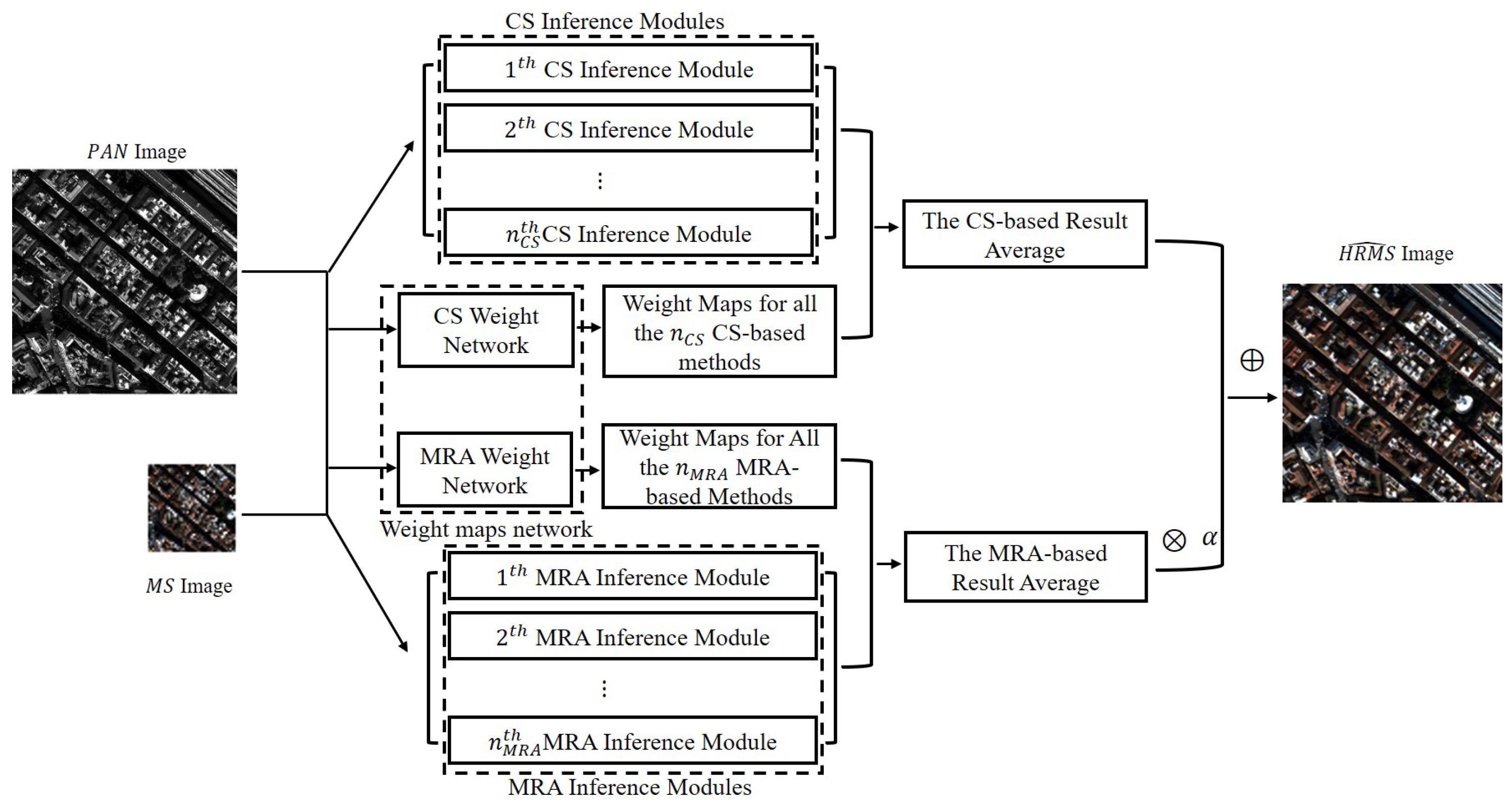
Figure 3.
Blockdiagram of the proposed PWNet for pansharpening. The proposed method can be divided into three independent part, i.e., the weight maps network, the CS inference modules and the MRA inference modules. The weight maps network takes the reduced MS and PAN image as inputs, and outputs weight maps for each of the CS-based and MRA-based methods. At the same time, the CS inference modules and the MRA inference modules generate HRMS images according to specific pansharpening methods. Finally, the estimated HRMS image is obtained by averaging all HRMS images estimated by the selected CS-based and MRA-based methods with the weight maps generated by the weight maps network.

Figure 4.
The architecture of proposed PWNet for generating the weight maps.

Figure 5.
Visual comparison of the CS-based and MRA-based methods and the proposed PWNet method on the WorldView-2 images, (a) PAN; (b) LRMS; (c) PCA; (d) GIHS; (e) Brovey; (f) BDSD; (g) GS; (h) GSA; (i) PRACS; (j) HPF; (k) SFIM; (l) Indusion; (m) AWLP; (n) ATWT-M3; (o) MTF-GLP-HPM; (p) MTF-GLP-CBD; (q) PWNet (ours); (r) Ground Truth.

Figure 6.
Visual comparison of the CS-based and MRA-based methods and the proposed PWNet method on the GeoEye-1 images, (a) PAN; (b) LRMS; (c) PCA; (d) GIHS; (e) Brovey; (f) BDSD; (g) GS; (h) GSA; (i) PRACS; (j) HPF; (k) SFIM; (l) Indusion; (m) AWLP; (n) ATWT-M3; (o) MTF-GLP-HPM; (p) MTF-GLP-CBD; (q) PWNet (ours); (r) Ground Truth.

Figure 7.
Visual comparison of the CS-based and MRA-based methods and the proposed PWNet method on the QuickBird images, (a) PAN; (b) LRMS; (c) PCA; (d) GIHS; (e) Brovey; (f) BDSD; (g) GS; (h) GSA; (i) PRACS; (j) HPF; (k) SFIM; (l) Indusion; (m) AWLP; (n) ATWT-M3; (o) MTF-GLP-HPM; (p) MTF-GLP-CBD; (q) PWNet (ours); (r) Ground Truth.

Figure 8.
Visualization of weight maps on the WorldView-2 images, (a) PCA; (b) BDSD; (c) PRACS; (d) AWLP; (e) MTF-GLP-HPM; (f) MTF-GLP-CBD.
Figure 8.
Visualization of weight maps on the WorldView-2 images, (a) PCA; (b) BDSD; (c) PRACS; (d) AWLP; (e) MTF-GLP-HPM; (f) MTF-GLP-CBD.

Figure 9.
Visualization of weight maps on the GeoEye-1 images, (a) PCA; (b) BDSD; (c) PRACS; (d) AWLP; (e) MTF-GLP-HPM; (f) MTF-GLP-CBD.
Figure 9.
Visualization of weight maps on the GeoEye-1 images, (a) PCA; (b) BDSD; (c) PRACS; (d) AWLP; (e) MTF-GLP-HPM; (f) MTF-GLP-CBD.

Figure 10.
Visualization of weight maps on the QuickBird images, (a) PCA; (b) BDSD; (c) PRACS; (d) AWLP; (e) MTF-GLP-HPM; (f) MTF-GLP-CBD.
Figure 10.
Visualization of weight maps on the QuickBird images, (a) PCA; (b) BDSD; (c) PRACS; (d) AWLP; (e) MTF-GLP-HPM; (f) MTF-GLP-CBD.

Figure 11.
Visual comparison of the CNN-based methods on the WorldVie-2 data set, (a) LRMS; (b) PNN; (c) DRPNN; (d) MSDCNN; (e) PWNet (ours); (f) Ground Truth.
Figure 11.
Visual comparison of the CNN-based methods on the WorldVie-2 data set, (a) LRMS; (b) PNN; (c) DRPNN; (d) MSDCNN; (e) PWNet (ours); (f) Ground Truth.

Figure 12.
Visual comparison of the CNN-based methods on the GeoEye-1 data set, (a) LRMS; (b) PNN; (c) DRPNN; (d) MSDCNN; (e) PWNet (ours); (f) Ground Truth.
Figure 12.
Visual comparison of the CNN-based methods on the GeoEye-1 data set, (a) LRMS; (b) PNN; (c) DRPNN; (d) MSDCNN; (e) PWNet (ours); (f) Ground Truth.

Figure 13.
Visual comparison of the CNN-based methods on the QuickBird data set, (a) LRMS; (b) PNN; (c) DRPNN; (d) MSDCNN; (e) PWNet(ours); (f) Ground Truth.
Figure 13.
Visual comparison of the CNN-based methods on the QuickBird data set, (a) LRMS; (b) PNN; (c) DRPNN; (d) MSDCNN; (e) PWNet(ours); (f) Ground Truth.

Figure 14.
Visual comparison of different methods on the WorldVie-2 data set at full resolution, (a) PCA; (b) GIHS; (c) Brovey; (d) BDSD; (e) GS; (f) GSA; (g) PRACS; (h) HPF; (i) SFIM; (j) Indusion; (k) AWLP; (l) ATWT-M3; (m) MTF-GLP-HPM; (n) MTF-GLP-CBD; (o) PNN; (p) DRPNN; (q) MSDCNN; (r) PWNet (ours).

Figure 15.
Visual comparison of different methods on the GeoEye-1 data set at full resolution, (a) PCA; (b) GIHS; (c) Brovey; (d) BDSD; (e) GS; (f) GSA; (g) PRACS; (h) HPF; (i) SFIM; (j) Indusion; (k) AWLP; (l) ATWT-M3; (m) MTF-GLP-HPM; (n) MTF-GLP-CBD; (o) PNN; (p) DRPNN; (q) MSDCNN; (r) PWNet (ours).

Figure 16.
Visual comparison of different methods on the QuickBird data set at full resolution, (a) PCA; (b) GIHS; (c) Brovey; (d) BDSD; (e) GS; (f) GSA; (g) PRACS; (h) HPF; (i) SFIM; (j) Indusion; (k) AWLP; (l) ATWT-M3; (m) MTF-GLP-HPM; (n) MTF-GLP-CBD; (o) PNN; (p) DRPNN; (q) MSDCNN; (r) PWNet (ours).


Table 1.
Information of the three data set.
| Satellite | Resolution of PAN | Resolution of MS | Number of Training Data Set | Number of Test Data Set |
|---|---|---|---|---|
| GeoEye-1 | 0.5 m | 2.0 m | 182 | 21 |
| WordView-2 | 0.5 m | 2.0 m | 224 | 32 |
| QuickBird | 0.6 m | 2.4 m | 529 | 60 |
Table 2.
Quantiative results obtained by PWNet with different .
| Q_avg | SAM | ERGAS | SCC | Q4 | |
|---|---|---|---|---|---|
| 0.1 | 0.9807 | 3.0250 | 2.5026 | 0.9831 | 0.9836 |
| 0.2 | 0.9825 | 2.9946 | 2.3140 | 0.9855 | 0.9854 |
| 0.3 | 0.9824 | 3.0216 | 2.2994 | 0.9858 | 0.9851 |
| 0.4 | 0.9831 | 2.9901 | 2.2947 | 0.9861 | 0.9856 |
| 0.5 | 0.9811 | 3.2168 | 2.3072 | 0.9854 | 0.9852 |
| 0.6 | 0.9807 | 3.3581 | 2.3935 | 0.9843 | 0.9854 |
| 0.7 | 0.9834 | 3.0276 | 2.2191 | 0.9866 | 0.9863 |
| 0.8 | 0.9831 | 3.0429 | 2.2504 | 0.9867 | 0.9859 |
| 0.9 | 0.9832 | 3.0543 | 2.2536 | 0.9862 | 0.9863 |
| 1 | 0.9493 | 3.2763 | 3.9663 | 0.9582 | 0.9546 |
Table 3.
Quantitative results and running time with different number of the averaged methods.
| and | Q_avg | SAM | ERGAS | SCC | Q4 | Time |
|---|---|---|---|---|---|---|
| 5 | 0.8781 | 5.9214 | 3.5179 | 0.8609 | 0.8761 | 0.3800 |
| 6 | 0.9079 | 5.7174 | 3.0616 | 0.9073 | 0.9062 | 0.5900 |
| 7 | 0.9209 | 5.1654 | 2.8986 | 0.9131 | 0.9165 | 0.9200 |
| 8 | 0.8781 | 5.4549 | 3.6942 | 0.8633 | 0.8615 | 1.6200 |
Table 4.
Results of the proposed PWNet with one shared weight map channel or four different weight map channels for each CS-based or MRA-based method. The best results are highlighted in bold.
Table 4.
Results of the proposed PWNet with one shared weight map channel or four different weight map channels for each CS-based or MRA-based method. The best results are highlighted in bold.
| Satellite | Number of Channels | Index | ||||
|---|---|---|---|---|---|---|
| Q_avg | SAM | ERGAS | SCC | Q4 | ||
| WordView-2 | 1 channel | 0.9874 | 2.7582 | 2.3830 | 0.9813 | 0.9805 |
| 4 channels | 0.3390 | 14.7379 | 14.2755 | 0.8378 | 0.8007 | |
| GeoEye-1 | 1 channel | 0.9207 | 4.2120 | 2.6868 | 0.9384 | 0.9117 |
| 4 channels | 0.3585 | 19.9451 | 14.5300 | 0.8141 | 0.5585 | |
| QuickBird | 1 channel | 0.8941 | 2.8252 | 1.8102 | 0.9480 | 0.8227 |
| 4 channels | 0.3442 | 19.6107 | 14.6745 | 0.8867 | 0.1462 | |
Table 5.
Quantitative comparison of the CS-based and MRA-based methods and the proposed PWNet method on the WorldView-2 images. The best and second best results are highlighted in bold.
Table 5.
Quantitative comparison of the CS-based and MRA-based methods and the proposed PWNet method on the WorldView-2 images. The best and second best results are highlighted in bold.
| Method | Q_avg | SAM | ERGAS | SCC | Q4 | |
|---|---|---|---|---|---|---|
| CS | PCA | 0.8885 | 5.3974 | 5.8650 | 0.9419 | 0.8705 |
| GIHS | 0.8858 | 5.6820 | 5.9937 | 0.9289 | 0.8777 | |
| Brovey | 0.8852 | 5.3037 | 5.9038 | 0.9357 | 0.8748 | |
| BDSD | 0.9709 | 4.4274 | 3.2701 | 0.9641 | 0.9628 | |
| GS | 0.8924 | 5.2195 | 5.7536 | 0.9428 | 0.8817 | |
| GSA | 0.9675 | 4.0382 | 3.6693 | 0.9542 | 0.9581 | |
| PRACS | 0.9224 | 4.5298 | 5.2480 | 0.9248 | 0.9143 | |
| MRA | HPF | 0.9454 | 4.1524 | 4.4125 | 0.9521 | 0.9372 |
| SFIM | 0.9498 | 4.2046 | 4.2015 | 0.9578 | 0.9426 | |
| Indusion | 0.8651 | 5.3162 | 6.4696 | 0.9025 | 0.8502 | |
| AWLP | 0.9617 | 3.7299 | 3.6508 | 0.9593 | 0.9529 | |
| ATWT-M3 | 0.8723 | 6.1898 | 6.5592 | 0.9067 | 0.8696 | |
| MTF-GLP-HPM | 0.9676 | 3.9731 | 3.5227 | 0.9607 | 0.9589 | |
| MTF-GLP-CBD | 0.9620 | 4.0397 | 3.4418 | 0.9575 | 0.9620 | |
| PWNet | 0.9836 | 3.5489 | 2.4584 | 0.9801 | 0.9723 |
Table 6.
Quantitative comparison of the CS-based and MRA-based methods and the proposed PWNet method on the GeoEye-1 images. The best and second best results are highlighted in bold.
Table 6.
Quantitative comparison of the CS-based and MRA-based methods and the proposed PWNet method on the GeoEye-1 images. The best and second best results are highlighted in bold.
| Method | Q_avg | SAM | ERGAS | SCC | Q4 | |
|---|---|---|---|---|---|---|
| CS | PCA | 0.8110 | 6.3414 | 4.8720 | 0.8544 | 0.8175 |
| GIHS | 0.8125 | 6.3189 | 4.8534 | 0.8539 | 0.8197 | |
| Brovey | 0.8063 | 6.5103 | 4.9593 | 0.8496 | 0.8120 | |
| BDSD | 0.9211 | 5.3528 | 3.8133 | 0.8721 | 0.9309 | |
| GS | 0.8119 | 6.3199 | 4.8650 | 0.8544 | 0.8188 | |
| GSA | 0.8959 | 6.3157 | 4.0425 | 0.8598 | 0.9079 | |
| PRACS | 0.8274 | 6.1486 | 4.7254 | 0.8483 | 0.8342 | |
| MRA | HPF | 0.8562 | 6.3038 | 4.4650 | 0.8596 | 0.8638 |
| SFIM | 0.8596 | 6.3688 | 4.4152 | 0.8599 | 0.8655 | |
| Indusion | 0.7518 | 7.1286 | 5.8135 | 0.7849 | 0.7579 | |
| AWLP | 0.8723 | 6.6096 | 4.3918 | 0.8548 | 0.8835 | |
| ATWT-M3 | 0.7193 | 7.9694 | 5.7994 | 0.8118 | 0.7218 | |
| MTF-GLP-HPM | 0.9016 | 6.3340 | 3.9931 | 0.8639 | 0.9108 | |
| MTF-GLP-CBD | 0.9198 | 6.3207 | 3.9122 | 0.8638 | 0.9198 | |
| PWNet | 0.9543 | 5.3245 | 2.8405 | 0.9380 | 0.9593 |
Table 7.
Quantitative comparison of the the CS-based and MRA-based methods and the proposed PWNet method on the QuickBird images. The best and second best results are highlighted in bold.
Table 7.
Quantitative comparison of the the CS-based and MRA-based methods and the proposed PWNet method on the QuickBird images. The best and second best results are highlighted in bold.
| Method | Q_avg | SAM | ERGAS | SCC | Q4 | |
|---|---|---|---|---|---|---|
| CS | PCA | 0.5754 | 7.4697 | 4.5931 | 0.7911 | 0.7165 |
| GIHS | 0.7965 | 4.2120 | 2.9488 | 0.9067 | 0.7906 | |
| Brovey | 0.8169 | 3.9059 | 2.7937 | 0.9187 | 0.8044 | |
| BDSD | 0.8977 | 4.2954 | 2.6979 | 0.9398 | 0.8906 | |
| GS | 0.7856 | 4.7382 | 3.1700 | 0.8874 | 0.7838 | |
| GSA | 0.8860 | 4.0225 | 2.5359 | 0.9252 | 0.8814 | |
| PRACS | 0.8510 | 3.8935 | 2.6258 | 0.9076 | 0.8319 | |
| MRA | HPF | 0.8856 | 3.8858 | 2.4156 | 0.9278 | 0.8778 |
| SFIM | 0.8902 | 3.8065 | 2.3617 | 0.9316 | 0.8818 | |
| Indusion | 0.7131 | 4.3943 | 3.5650 | 0.8664 | 0.7004 | |
| AWLP | 0.9068 | 3.5775 | 2.2182 | 0.9425 | 0.8982 | |
| ATWT-M3 | 0.8059 | 4.5073 | 2.9060 | 0.8982 | 0.7912 | |
| MTF-GLP-HPM | 0.9056 | 3.7543 | 2.3366 | 0.9378 | 0.8985 | |
| MTF-GLP-CBD | 0.8877 | 4.0365 | 2.5360 | 0.9261 | 0.8877 | |
| PWNet | 0.9196 | 3.5275 | 2.1635 | 0.9431 | 0.9109 |
Table 8.
Quantitative comparison of the CNN-based methods on three test data sets. The best results are highlighted in bold.
Table 8.
Quantitative comparison of the CNN-based methods on three test data sets. The best results are highlighted in bold.
| Method | Q_avg | SAM | ERGAS | SCC | Q4 | |
|---|---|---|---|---|---|---|
| WorldView-2 | PNN | 0.9479 | 5.2180 | 5.1040 | 0.8975 | 0.9256 |
| DRPNN | 0.9292 | 4.4765 | 5.3072 | 0.8887 | 0.9030 | |
| MSDCNN | 0.9443 | 4.4135 | 6.8478 | 0.9407 | 0.8512 | |
| PWNet | 0.9874 | 2.7582 | 2.3830 | 0.9813 | 0.9805 | |
| GeoEye-1 | PNN | 0.8639 | 4.8190 | 3.5224 | 0.8888 | 0.8435 |
| DRPNN | 0.7934 | 4.8685 | 3.7746 | 0.8931 | 0.7733 | |
| MSDCNN | 0.8462 | 4.9707 | 3.3115 | 0.9093 | 0.8518 | |
| PWNet | 0.9207 | 4.2120 | 2.6868 | 0.9384 | 0.9117 | |
| QuickBird | PNN | 0.7047 | 3.3113 | 2.6980 | 0.9258 | 0.5950 |
| DRPNN | 0.7648 | 2.4289 | 1.7544 | 0.9473 | 0.7750 | |
| MSDCNN | 0.7727 | 2.7034 | 1.8429 | 0.9450 | 0.7845 | |
| PWNet | 0.8258 | 2.2163 | 1.5525 | 0.9644 | 0.8234 |
Table 9.
Performance comparison on three test data sets at full resolution. The best and second best results are highlighted in bold and underlined, respectively.
Table 9.
Performance comparison on three test data sets at full resolution. The best and second best results are highlighted in bold and underlined, respectively.
| GeoEye-1 | WorldView-2 | QuickBird | |||||||
|---|---|---|---|---|---|---|---|---|---|
| Methed | QNR | QNR | QNR | ||||||
| PCA | 0.1020 | 0.1542 | 0.7595 | 0.0265 | 0.2143 | 0.7649 | 0.0527 | 0.1036 | 0.8491 |
| GIHS | 0.0347 | 0.1812 | 0.7903 | 0.0767 | 0.0845 | 0.8453 | 0.0819 | 0.0815 | 0.8432 |
| Brovey | 0.0337 | 0.1769 | 0.7954 | 0.0377 | 0.1008 | 0.8653 | 0.0545 | 0.0577 | 0.8910 |
| BDSD | 0.2103 | 0.3887 | 0.4827 | 0.1016 | 0.2569 | 0.6676 | 0.2748 | 0.3250 | 0.4895 |
| GS | 0.0379 | 0.1816 | 0.7873 | 0.0167 | 0.1049 | 0.8802 | 0.0443 | 0.0613 | 0.8971 |
| GSA | 0.2925 | 0.1226 | 0.6207 | 0.1079 | 0.1444 | 0.7633 | 0.0940 | 0.1126 | 0.8040 |
| PRACS | 0.0587 | 0.1533 | 0.7970 | 0.0231 | 0.0908 | 0.8882 | 0.0492 | 0.0845 | 0.8704 |
| HPF | 0.1500 | 0.2023 | 0.6780 | 0.0533 | 0.1028 | 0.8494 | 0.0603 | 0.0515 | 0.8913 |
| SFIM | 0.1469 | 0.1971 | 0.6849 | 0.0532 | 0.0974 | 0.8546 | 0.0587 | 0.0517 | 0.8926 |
| Indusion | 0.0867 | 0.1126 | 0.8105 | 0.0312 | 0.0544 | 0.9161 | 0.0691 | 0.0444 | 0.8895 |
| AWLP | 0.1621 | 0.1914 | 0.6776 | 0.0437 | 0.0908 | 0.8695 | 0.0575 | 0.0583 | 0.8875 |
| ATWT-M3 | 0.1198 | 0.1782 | 0.7234 | 0.0617 | 0.0818 | 0.8615 | 0.0588 | 0.0806 | 0.8653 |
| MTF-GLP-HPM | 0.1810 | 0.1986 | 0.6563 | 0.0604 | 0.1096 | 0.8366 | 0.0827 | 0.0675 | 0.8554 |
| MTF-GLP-CBD | 0.2199 | 0.2009 | 0.6234 | 0.0752 | 0.1282 | 0.8062 | 0.0800 | 0.0673 | 0.8580 |
| PNN | 0.1042 | 0.0404 | 0.8596 | 0.0636 | 0.0322 | 0.9062 | 0.0306 | 0.0490 | 0.9218 |
| DRPNN | 0.0268 | 0.0764 | 0.8988 | 0.0359 | 0.0636 | 0.9027 | 0.0199 | 0.0954 | 0.8866 |
| MSDCNN | 0.0699 | 0.0795 | 0.8562 | 0.0282 | 0.0734 | 0.9004 | 0.0946 | 0.1068 | 0.8087 |
| PWNet | 0.0289 | 0.1127 | 0.8616 | 0.0172 | 0.0700 | 0.9139 | 0.0428 | 0.0559 | 0.9037 |
Table 10.
Running time comparison of different methods (in second).
| Method | Time | Methed | Time |
|---|---|---|---|
| PCA | 0.0900 | Indusion | 0.0600 |
| GIHS | 0.0100 | AWLP | 0.0400 |
| Brovey | 0.0010 | ATWTM3 | 0.1100 |
| BDSD | 0.2700 | MTF_GLP_HPM | 0.0400 |
| GS | 0.0300 | MTF_GLP_CBD | 0.0500 |
| GSA | 0.1000 | PNN | 0.5900 |
| PRACS | 0.1000 | DRPNN | 6.5100 |
| HPF | 0.0100 | MSDCNN | 1.9900 |
| SFIM | 0.0100 | PWNet | 1.0200 |
© 2020 by the authors. Licensee MDPI, Basel, Switzerland. This article is an open access article distributed under the terms and conditions of the Creative Commons Attribution (CC BY) license (http://creativecommons.org/licenses/by/4.0/).
Share and Cite
MDPI and ACS Style
Liu, J.; Feng, Y.; Zhou, C.; Zhang, C. PWNet: An Adaptive Weight Network for the Fusion of Panchromatic and Multispectral Images. Remote Sens. 2020, 12, 2804. https://doi.org/10.3390/rs12172804
AMA Style
Liu J, Feng Y, Zhou C, Zhang C. PWNet: An Adaptive Weight Network for the Fusion of Panchromatic and Multispectral Images. Remote Sensing. 2020; 12(17):2804. https://doi.org/10.3390/rs12172804
Chicago/Turabian StyleLiu, Junmin, Yunqiao Feng, Changsheng Zhou, and Chunxia Zhang. 2020. "PWNet: An Adaptive Weight Network for the Fusion of Panchromatic and Multispectral Images" Remote Sensing 12, no. 17: 2804. https://doi.org/10.3390/rs12172804
Note that from the first issue of 2016, this journal uses article numbers instead of page numbers. See further details here.