Article

Improving the Accuracy of Multiple Algorithms for Crop Classification by Integrating Sentinel-1 Observations with Sentinel-2 Data

by
Amal Chakhar
,
David Hernández-López
,
Rocío Ballesteros
and
Miguel A. Moreno
*
Institute of Regional Development, University of Castilla-La Mancha, 02071 Albacete, Spain
*
Author to whom correspondence should be addressed.
Remote Sens. 2021, 13(2), 243; https://doi.org/10.3390/rs13020243
Submission received: 6 December 2020 / Revised: 21 December 2020 / Accepted: 8 January 2021 / Published: 12 January 2021

Abstract

:
The availability of an unprecedented amount of open remote sensing data, such as Sentinel-1 and -2 data within the Copernicus program, has boosted the idea of combining the use of optical and radar data to improve the accuracy of agricultural applications such as crop classification. Sentinel-1’s Synthetic Aperture Radar (SAR) provides co- and cross-polarized backscatter, which offers the opportunity to monitor agricultural crops using radar at high spatial and temporal resolution. In this study, we assessed the potential of integrating Sentinel-1 information (VV and VH backscatter and their ratio VH/VV with Sentinel-2A data (NDVI) to perform crop classification and to define which are the most important input data that provide the most accurate classification results. Further, we examined the temporal dynamics of remote sensing data for cereal, horticultural, and industrial crops, perennials, deciduous trees, and legumes. To select the best SAR input feature, we tried two approaches, one based on classification with only SAR features and one based on integrating SAR with optical data. In total, nine scenarios were tested. Furthermore, we evaluated the performance of 22 nonparametric classifiers on which most of these algorithms had not been tested before with SAR data. The results revealed that the best performing scenario was the one integrating VH and VV with normalized difference vegetation index (NDVI) and cubic support vector machine (SVM) (the kernel function of the classifier is cubic) as the classifier with the highest accuracy among all those tested.

1. Introduction

Thanks to the development of Earth Observation (EO) technologies, remotely sensed data have become accessible for a broad range of users in both the public and private sector and cover many important application domains [1], such as protecting fragile ecosystems, managing climate risks, and enhancing food security [2]. Therefore, data derived from EO information are becoming indispensable in support of many sectors of society, especially for agronomic applications. Indeed, remote sensing data derived from EO have already proven their potential and effectiveness in spatiotemporal vegetation monitoring [3,4]; therefore, monitoring agricultural resources using remote sensing offers the opportunity to estimate crop areas [5], predict crop yield [6,7,8], and evaluate water demand [9,10] and to know the total surface that is cultivated and the precise distribution of crops [11]. Accordingly, in order to establish the most effective management strategy and adapt agricultural practices correspondingly, regular precise information is required to find out variations in the field, so that policymakers, stakeholders, farmers, and researchers can be informed about the state of agricultural land. Crop classification is one of the most used methods of information extraction to manage and plan many agricultural activities.
However, the above-mentioned applications are still mostly based on optical remote sensing [12]. Commonly, the optical remote sensing methods used to assess crop status rely on combinations of different bands that are used to build relationships with crop biophysical parameters of the canopy [13]. Unfortunately, according to [14], two-thirds of the EO provided data by optical remote sensing sources are often covered by clouds throughout the year. Hence, it may be a challenge to overcome weather conditions with the objective of obtaining an acceptable quality of optical remote sensing data. For this reason, [12] listed out the advantages that synthetic aperture radar (SAR) data have over optical data, and it can be resumed into three main characteristics. The first one concerns the ability of SAR sensors to acquire data independently of the weather condition and at night [15]. The second important property is the sensitivity of SAR data to canopy structure [16,17]. The third characteristic concerns the SAR sensitivity to moisture or the water content of the land surface [18,19,20,21,22,23]. Nevertheless, dealing with radar data for any land application is a challenging task and many consideration should be taken into account, such as removing the speckle noise effect from radar images [24,25], and dealing with the difficulty in interpreting the information [26] and the distortion caused by changes in topography [27].
To make the most of the aforementioned advantages of SAR data, several authors considered using them for phenological monitoring of numerous crop types and had very promising results. One study [28] found that the synergistic integration of SAR and optical time series offers an unprecedented opportunity in vegetation phenology monitoring for mountain agriculture management. The central idea of this work was to derive the main phenological features from time series of Sentinel-1 and Sentinel-2 images. Results show that Sentinel-1 cross-polarized VH backscattering coefficients have a strong vegetation contribution and are well correlated with the normalized difference vegetation index (NDVI) values retrieved from optical sensors, thus allow the extraction of meadow phenological phases. Likewise, another study [29] analyzed the temporal trajectory of SAR and optical remote sensing data for a variety of winter and summer crops widely cultivated in the world (wheat, rapeseed, maize, soybean, and sunflower). The SAR backscatter and NDVI temporal profiles of fields with various management practices and environmental conditions were interpreted physically. Accompanied by some in situ measurements (Green Area Index (GAI) and fresh biomass) as well as rainfall and temperature data, the time series of optical NDVI and SAR backscatter (VH, VV, and VH/VV) were analyzed and physically interpreted. As a result, this study pointed out that dense time series allowed the capture of short phenological stages and, thus, precise descriptions of various crop developments.
Therefore, SAR data may offer valuable information that can reinforce optical remote sensing data and can be especially advantageous to crop classification application. That is the reason why several classification studies used both SAR and optical remote sensing products [30,31,32] in order to assess the potential of their complementary use. For instance, a study was carried out with the objective of joining the use of Sentinel-1 radar and Sentinel-2 optical imagery to create a crop map for Belgium [33]. The obtained results showed that the combination of radar and optical imagery outperformed classification based on single-sensor inputs. These results were obtained following a methodology that highlighted the role of each remote sensing component. This procedure relied on the use of 18 incremental classification schemes, and the classification was performed by a random forest (RF) classifier. Another work [34] used 9 Sentinel-1 SAR images and 11 optical Landsat-8 images (used as a surrogate for Sentinel-2). Further, classification was done by the RF classifier and the methodology was set to highlight the impact of SAR image time series when they were used as a complement to optical imagery. In addition, this work evaluated the most relevant SAR image features and the use of temporal gap-filling of the optical image time series. The study presented two main conclusions. First, SAR image time series allowed significant improvements in the classification process, and second, they allowed the use of optical data without a gap-filling process, because a methodology was used to replace the missing values that were eliminated by a cloud screening filter [35]. In agreement with the previous studies, it was revealed in [36] that the synergic use of Sentinel-1 and Landsat-8 data enhanced the accuracy of classifications compared to those performed with optical or radar images alone. Moreover, the classification in this study was performed by RF. Furthermore, a series of studies was conducted in [37] to improve the classification efficiency in cloudy and rainy regions using Sentinel-1 and Landsat-8, but they built a recurrent neural network (RNN)-based classifier suitable for remote sensing images on the geo-parcel scale. They succeeded in designing an improved crop planting structure map in their specific study area.
The current work is based on the results reported in [
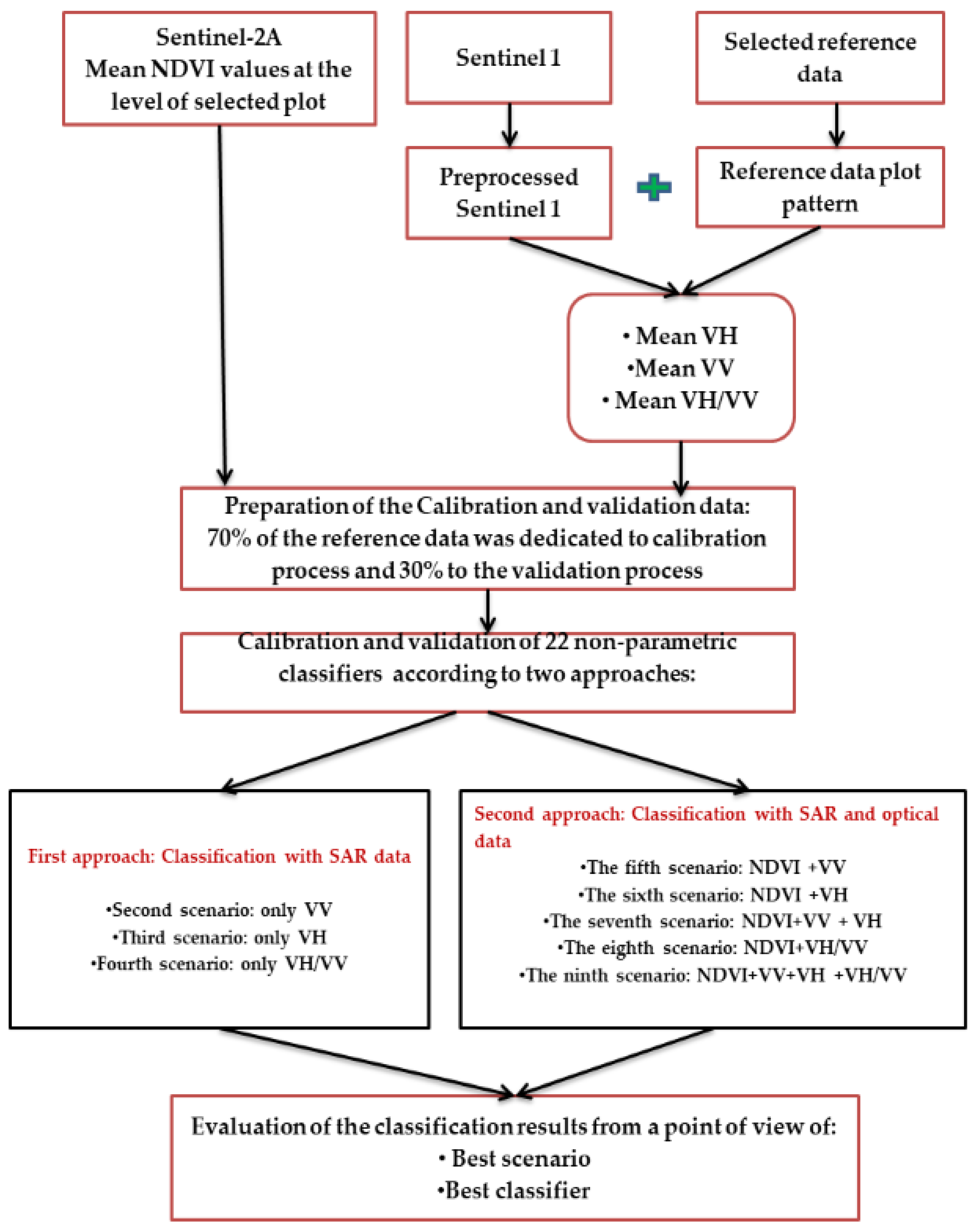
38], the main objective of which was to assess the contribution of Sentinel-2A and Landsat-8 information to crop classification. Moreover, 22 classification algorithms were evaluated to determine which was the most robust. The use of combined Sentinel-2A and Landsat-8 information did not contribute much to improve crop classification accuracy compared with using only Sentinel-2A information. Further, large differences in accuracy were found depending on the machine learning algorithm that was used, which also depends on the type of information used. Consequently, the interest of the present work is in integrating multitemporal SAR data, Sentinel-1, and optical data obtained with Sentinel-2A, together with determining the best machine learning algorithm to perform accurate crop classification in a semiarid region. The following are the main objectives:
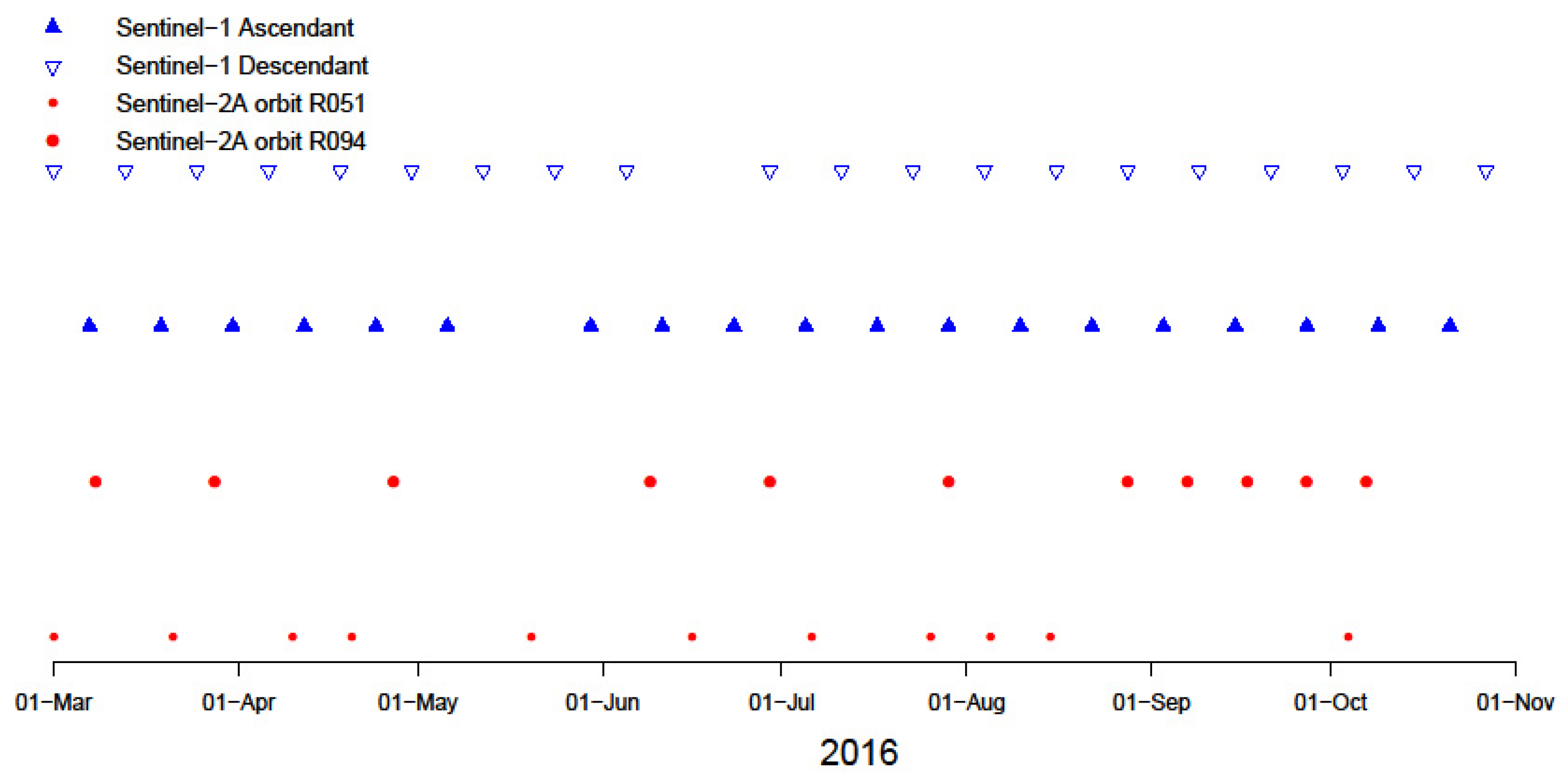
Establish a simple and efficient methodology that allows the incorporation of SAR data with optical data to perform classification over a large area and with a dense time-series of Sentinel-2 (22 different acquisition date) and Sentinel-1 (39 different acquisition date) data, so that the phenological temporal dynamics of the studied crops can be detected completely, with the purpose to provide the maximum amount of information that allow the differentiation between the crops.
Select the best SAR feature that allows the best classification results.
Evaluate the performance of 22 nonparametric classifiers that were tested in our previous work with only optical data. In this current work we added SAR data to the optical. The novelty that this paper can bring is that a large number of these algorithms have not been tested with SAR data, so depending on their performance, we will assess them and select the best one.

2. Materials and Methods

2.1. Study Area

The study area covers the agricultural fields in the province of Castilla-La Mancha, southeast Spain (Figure 1). It is located in the south of the north temperate zone, although it presents a continental nature due to its mean elevation (700 ma.s.l.) and distance from sea. Farmland is the most common type of land use in the study area The most limiting factor for farming is the weather. This area is classified as semiarid (aridity index (AI) 0.26). Annual reference evapotranspiration values (ETo) are from 1165 mm year−1 in the central area of the aquifer to more than 1300 mm year−1 in the northwest and southeast. Agro-climatic stations showed precipitation values from 336 to 413 mm year−1 with a maximum value of 82 mm in summertime. The analysis of thermal characteristics shows variations from 19.3 to 20.8 °C for annual mean daily maximum temperature and from 6.3 to 6.6 °C for annual mean daily minimum temperatures. The proposed methodology was carried out in area spread over a surface equal to 7200 km2. This extension can be considered a wide area that can provide trustful results compared with other studies performed in smaller areas [39,40,41,42,43].

2.2. Sentinel-1 and -2 Datasets

2.2.1. Sentinel-2A Dataset

Sentinel-2A products were acquired in 22 different occasion (Figure 2) during the period March–October 2016. For each acquisition date we downloaded three different Sentinel-2A tiles SXJ, SWJ and SWH (Figure 3) to cover the whole study area. The Sentinel-2A products were downloaded from the European Space Agency (ESA) Copernicus Open Access Hub subsequently were atmospherically corrected using Sen2cor algorithm implemented in the Sentinel Application Platform (SNAP).Then, our selected vegetation Index VI was the normalized difference vegetation index NDVI, because it is the most widespread used VI in the literature and very accurate in the monitoring of the crop phenology. NDVI at the bottom of the atmosphere (NDVIBOA) was calculated as the following equation:
N D V I B O A   =   Band   8 Band   4   Band   8 + Band   4

2.2.2. Sentinel-1A Dataset

A total of 39 Sentinel-1 images were acquired between March and October 2016 (Figure 2). The Sentinel-1 dataset comprises Level-1 Ground Range Detected (GRD) data in Interferometric Wide (IW) swath mode that was projected to ground range using the WGS84 Earth ellipsoid model. The resulting images in dual polarization (VH and VV) had dimensions of 270 × 270 km, resolution of 10 m, and temporal resolution of 6 to 12 days. (Images were downloaded from https://earthdata.nasa.gov/eosdis/daacs/asf.) All images were processed by SNAP using the Sentinel-1 toolbox.
For all Sentinel-1 images, the study site was imaged with an incidence angle (θ) in range of 35° to 41°. According to [29], incidence angles between 38° and 41° are appropriate for crop parameter retrieval, because angles 35–40° increase the path length through vegetation and maximize the vegetation scattering contribution [44], while steep incidence angles <30° reduce the vegetation attenuation and maximize the ground scattering contribution. In order to obtain Sentinel-1 images useful for the classification process, a series of steps must be taken:
  • Orbit correction: This first correction is applied in the case where the orbit state vector is not accurate. Performing this correction allows the automatic download and update of the orbit state vectors, providing an accurate satellite position and velocity information [45].
  • Radiometric calibration: The purpose of radiometric calibration is to convert the digital number DN values of Sentinel-1 images into backscattering coefficients (σ°) [46]. Radiometric calibration was applied according to the following equation [47]:
    v a l u e ( i )   =   | DN i 2 + b | Ai
    where Ai i is the sigmaNought(i), calibration vector (i), and b is a constant offset [47].
  • Speckle filtering: Speckle is random “salt-and-pepper” noise that deteriorates the image quality [48] and affects the understanding of backscatter responses from surface features. The refined Lee filter [49] was applied to attenuate the speckle effect.
  • Geometric correction: Topographic variations of scenes and the inclination of the radar sensor generate distortions in the image. Therefore, performing geometric correction can mitigate the distortion effect [46]. Range Doppler terrain correction, through SNAP, was applied for this correction.
  • Conversion to decibel units: The backscatter coefficient σ 0 , which is on a linear scale, is converted to the decibel (db) scale, σ 0 ( db )   =   10 log 10 σ 0 , where σ 0 (db) represents the backscatter coefficient value in decibels.
The mean backscattering coefficient was calculated from the processed Sentinel-1 images by averaging the σ° values of all pixels at the level of each reference crop.

2.3. Overview of the Methodology

As mentioned in the Introduction, the objective of this study is to evaluate the effectiveness of incorporating Sentinel-1 data with Sentinel-2A optical remote sensing data for crop classification. Further, it was reported that the main methodology line of this work is based on [38], except that in that work the optical sources of information were Sentinel-2A and Landsat-8; in the present work we used only Sentinel-2A data, because it was concluded that integrating Landsat-8 with Sentinel-2A did not bring important improvements compared to using only Sentinel-2A data in the classification. Additionally, we evaluated the performance of the 22 nonparametric classifiers by integrating SAR data, because the type of data determines the selection of the best algorithm. We applied the developed methodology to the exact same case study in order to eliminate any bias in the analysis of the contribution of SAR data to classification with only optical data. The adapted methodology was as follows (Figure 4).

2.3.1. Data Collection

We obtained optical and SAR data from March to October 2016. Concerning reference data, they were obtained from the field visits performed by the Confederación Hidrográfica del Júcar, Spain (www.chj.es) during the irrigation season of 2016. They visited 6341 plots that covered 28, 963 ha. In our previous work [38] we used only plots with an area larger than 1 ha because we used Landsat 8 and Sentinel-2A data, and given that Landsat 8 have a spatial resolution equal to 30 m so we performed a spatial analysis to select the reference plots. This spatial analysis consisted in eliminating plots with a size area less than 1 ha, to ensure that there was a sufficient number of pixels inside each plot (3pixels×3 pixels for Landsat-8). To select reference data with pixels that were completely inside the plot, also to avoid a border effect, a buffer of 30 m inside the plot was implemented. Consequently, the number of used plots was reduced to 3111 (24,208 ha), and given that we want to compare the classification results of the previous work with the results of the actual work we decided to preserve our previous reference data selection.
According to the climatic condition of the study area, we can found four groups of crops with different culture systems: (1) cold weather crops that are sown in the autumn or early winter and are harvested at the end of spring or at the beginning of summer; (2) warm season crops for which the growing cycle develops in the summer; (3) rain-fed crops that are limited by the rainfall regimes; and (4) irrigated crops. For example, a crop distribution in 2012 included 14.2% wheat, 14.0% barley, 7.1% maize, 5.8% woody crops, 5.6% opium, 4.9% garlic, 4.4% alfalfa, 3.9% onion, garlic, pea, double crops, and other vegetables. Therefore, basing on the main crop distribution in the area, the following land cover class were selected: cereals (barley C1, maize C2, and wheat C3), horticultural crops (onion C4, purple garlic C5, and white garlic C6), industrial crops (poppy C7 and sunflower C8), perennials (alfalfa C9), deciduous trees (almond C10 and grapevines C11), and legumes (peas C12).

2.3.2. Data Preparation

Once the SAR data were acquired, they had to be preprocessed in order to extract useful information for the classification process (more details are given in the Sentinel-1 preprocessing section). Prior to the preprocessing process, we extracted three features from the Sentinel-1 dataset: VH, VV, and the VH/VV ratio. We computed the mean of these features at the level of plot (plot-based approach) for each available date of Sentinel-1 time series. Concerning the optical data, the selected vegetation index NDVI was calculated also at the level of each reference plot.

2.3.3. Classification Process

Given that one of the critical issues in using SAR time series is the choice of features used for classification, we decided to evaluate all selected SAR features from the previous step over two approaches. In the first approach, each feature was in a separate scenario, with the purpose of studying the classification results with only SAR data and comparing them with the results using optical data. The second approach was about combining these features with the NDVI. Nine classification scenarios based on the selected input feature were then applied for all available dates from March to October.
It is important to mention that the first scenario is considered the reference scenario. It had NDVI (calculated from Sentinel-2A bands) as an input feature. This decision was made because we wanted to compare it with the results of classification performed entirely with SAR data and detect the added value that SAR features can bring to classical classification methodology (which is based on only optical data).
First approach: classification with only SAR data. The scenarios of the first approach are in Table 1.
Second approach: classification with SAR and optical data. The scenarios of the second approach are in Table 2.
As stated above, the 22 nonparametric classifiers evaluated using optical and combined optical and SAR data. The algorithms evaluated are those included in the Classification Learner application of Matlab® (Table 3). In Table 3 we presented the names of these classifiers, their abbreviations, and the groups they belong to. We calibrated and evaluated the performance of these 22 nonparametric algorithms by applying the aforementioned scenarios.
Decision Trees DT is a non-parametric supervised learning method. DT takes a set of features as input, and returns an output through a sequence of tests. Trees build the rule by recursive binary partitioning regions (nodes) that are increasingly homogeneous with respect to their class variable [50]. DT classifiers create multivariate models based on a set of decision rules defined by combinations of features and a set of linear discriminant functions that are applied at each test node [51].
Discriminant analysis, is also known as the Fisher discriminant, named for its inventor, Sir R. A. Fisher [52], is a classification method. It assumes that different classes generate data based on different Gaussian distributions. To train a classifier, the fitting function estimates the parameters of a Gaussian distribution for each class. To predict the classes of new data, the trained classifier finds the class with the smallest misclassification cost.
An SVM classifies data by finding the best hyperplane that separates all data points of one class from those of the other class [53]. The best hyperplane for an SVM means the one with the largest margin between the two classes. Margin means the maximal width of the slab parallel to the hyperplane that has no interior data points.
The idea of K-Nearest Neighbors (KNN) is that one uses a large amount of training data, where each data point is characterized by a set of variables. Theoretically, each point is plotted in a high-dimensional space, where each axis in the space corresponds to an individual variable. When a new (test) data point is introduced, the algorithm tries to find out the K nearest neighbors that are closest. The number K is typically chosen as the square root of N, the total number of points in the training data set [54]. An ensemble consists of a set of individually trained classifiers (such as neural networks or decision trees) whose predictions are combined when classifying to obtain better predictive performance. An ensemble is itself a supervised learning algorithm, because it can be trained and then used to make predictions. Many researchers have examined the technique of combining the predictions of multiple classifiers to produce a single classifier [55]. The resulting classifier (the ensemble) is generally more accurate than any of the individual classifiers making up the ensemble. Both theoretical and empirical [56] research has demonstrated that a good ensemble is one where the individual classifiers in the ensemble are both accurate and make their errors on different parts of the input space. Two popular methods for creating accurate ensembles are Bagging [57] and Boosting [58]. Bagging is to have multiple classifiers trained on different under-sampled subsets and allow these classifiers to vote on a final decision, contrasting with just using one classifier [57]. The number of component classifiers of an ensemble has a great impact on the accuracy of prediction.

2.3.4. Quality Assessment

A calibration–validation procedure was implemented. The split in calibration and validation was as following: 70% of the reference data was dedicated to calibration process and 30% to the validation process. A confusion matrix of classical performance indicators of producer’s accuracy (PA), user’s accuracy (UA), and F1 score was generated to carry out the evaluation.
Producer’s accuracy PA results from dividing the number of correctly classified plots in each class (on the major diagonal) by the number of reference plots to be of that class (the column total) [59]. User’s accuracy UA can be simply computed by dividing the number of correctly classified plots in each class by the total number of plots that were classified for that class (the total row) [59].
The weighted F1 score statistic was used for classification algorithm selection [60] and this accuracy metrics was calculated using a Python library called Scikit-Learn. F1 score was calculated according to the following equation:
F 1   s c o r e   =   2 ( Precision     Recall ) / ( Precision   +   Recall )
where Precision gives the measure of correctly predicted class values over the total predicted class values. Recall is a ratio of correctly predicted class values to the actual class values.

3. Results

3.1. Analysis of Temporal Signatures of Crops
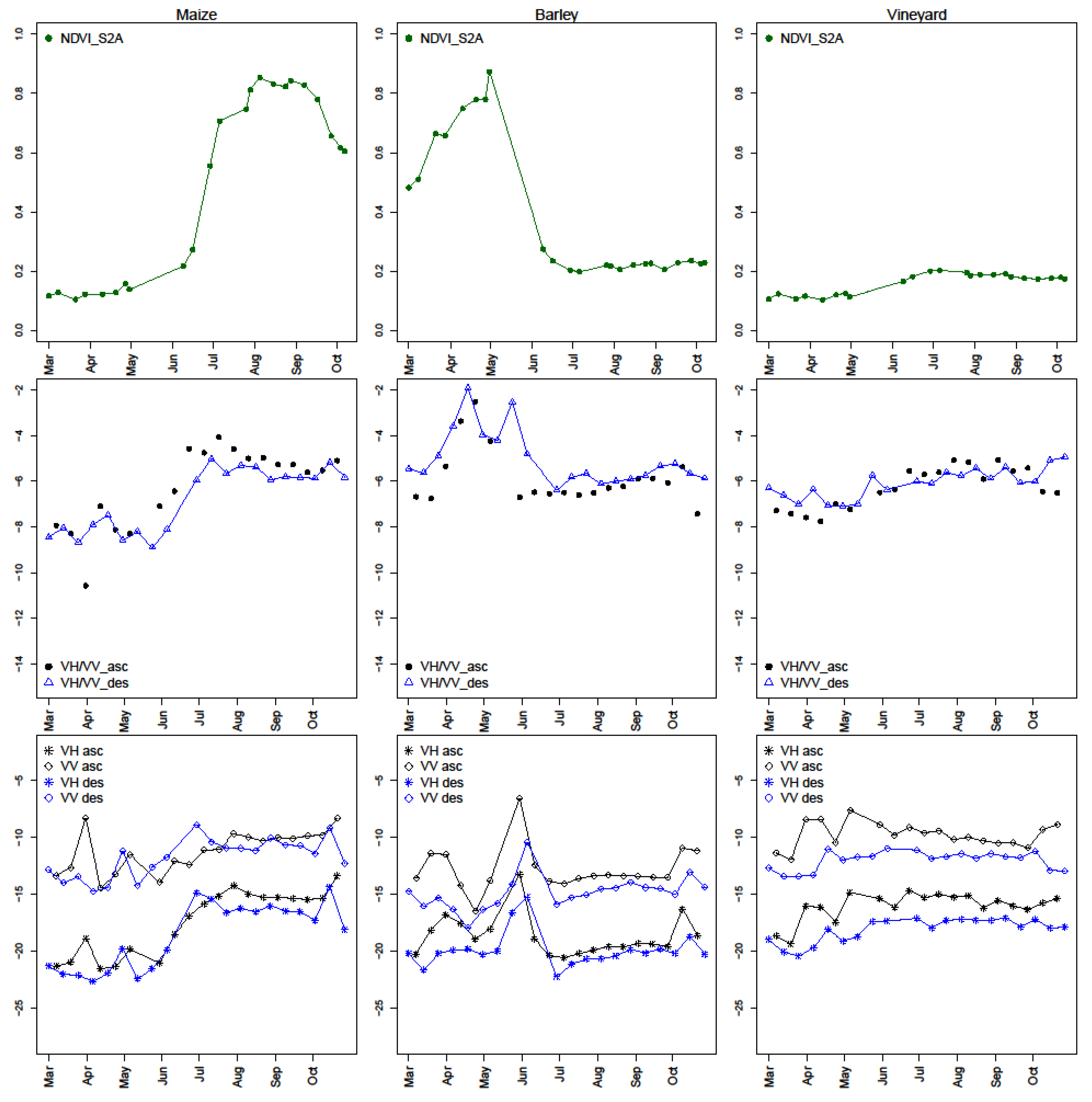
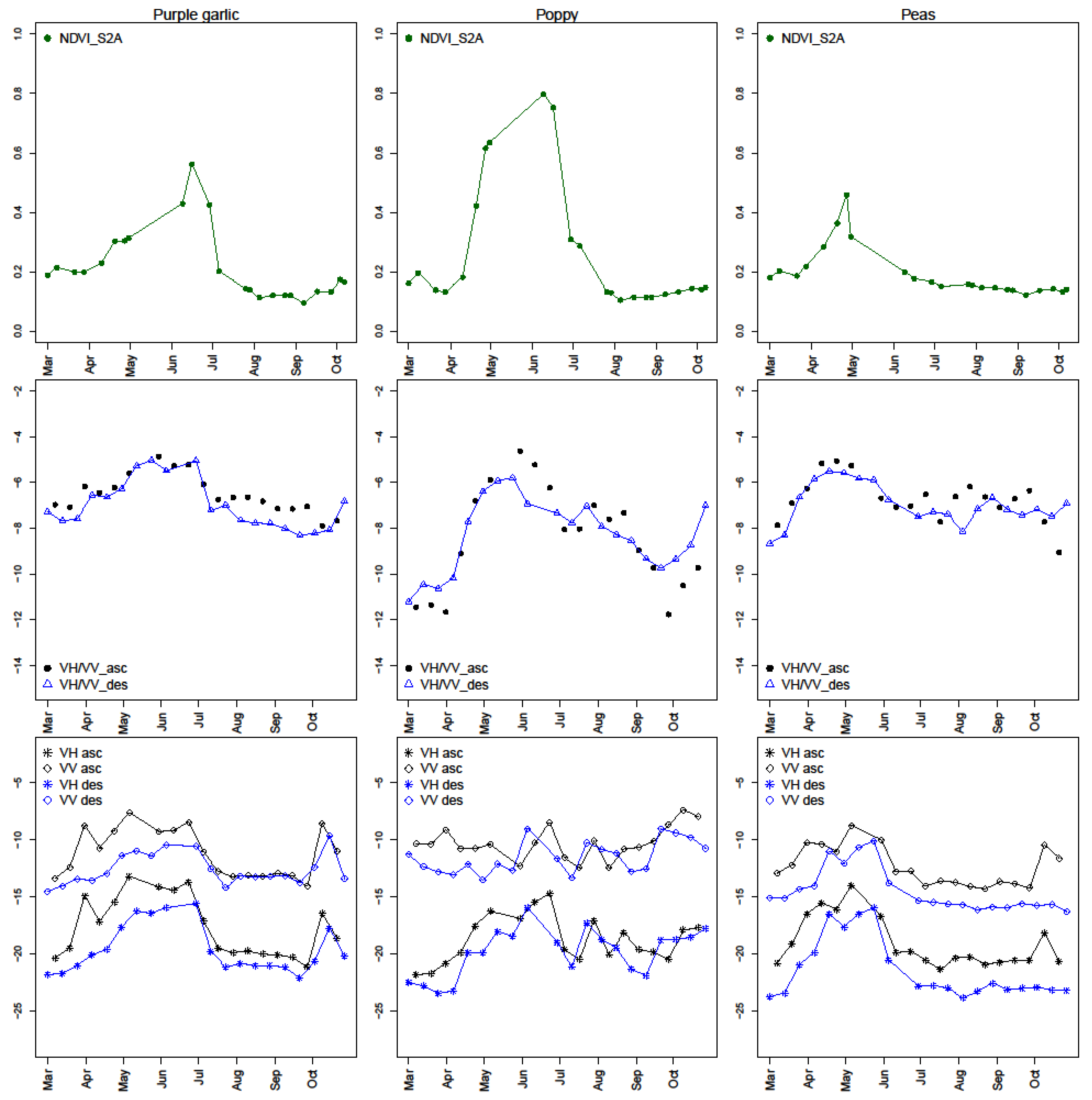
Figure 5 and Figure 6 represent the NDVI profile and temporal signatures of six of the studied crops for the three backscatter channels (VH, VV, and VH/VV) of descendant and ascendant orbits. We decided to comment briefly on the general tendency of the selected crops.
As a general observation for all crop types, the curves of both ascendant and descendant orbits have the same general tendency.
When considering the maize crop (
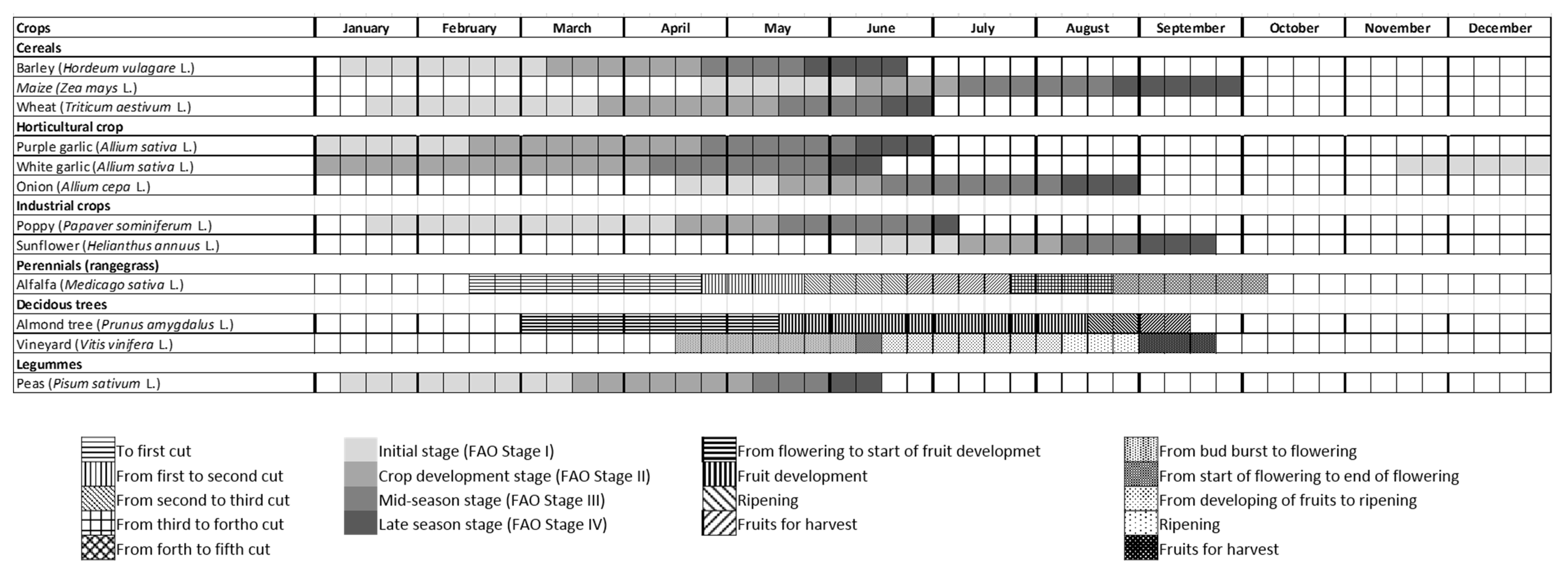
Figure 5, left column), generally in the study area it is sown in April and the harvest period can extend from the end of August to the end of September (Figure 7). From 15 May to the start of July, the VH backscatter and VH/VV steadily increased. According to [61], this observation can be explained by an increase in volume scattering when newly formed leaves are unfold, and subsequently by the accumulation of biomass. VV also rises constantly during the vegetation development phase. This increase may be due to the augmentation in double bounce scattering [62]. During the ripening phase, from mid-July to the end of September, it can be noticed that VH/VV, VH, and VV remain stable, indicating that maize reaches its maximum height and the fruit is in the development phase [61].
In the case of barley (Figure 5, center column), in this study area it is seeded at the start of January and harvested at the end of June or beginning of July (Figure 7). It is important to mention that barley and wheat have very similar growing seasons, phenology, and crop structure [63]. At the early and late growth stages, when the crop emerges and after the harvest, the backscatter is essentially determined by the condition of the soil, but between the start and end of the growth cycle, vegetation scattering becomes significant and the relationship between radar backscatter and vegetation biophysical parameters is considerably influenced by the dynamics of the canopy structure, including orientation, size, and density of the stems, and the dielectric constant of the crop elements, which depends on the phenological stage [29,64]. Vegetation starts to increase at the beginning of March, which corresponds to the tillering stage until the beginning of April, which corresponds to the stem elongation period. So, as consequence of this vegetation development, VH and VV increase, while from 10 to 15 April, both backscatter signals decrease due to the rising attenuation from the predominantly vertical structure of the barley stems [29,63]. At the beginning of May, we again observed an increase in VH and VV polarization, which is related to the heading stage [65,66], and this can be explained by the increase in fresh biomass. VH/VV starts to increase at the tillering phase (beginning of March) and continues to rise during the stem extension phase (corresponding to the period 20 March to 10 April). Further, a decrease is noticed from 10 April until the start of May, related with VH and VV to the vertically rising structure of the crop, as commented previously. Around the start of May, the VH/VV ratio starts to increase again, indicating the start of the heading and flowering phase. As heading takes place, the flag leaves become less dominant within the canopy, and as a consequence, the crop develops a more open vertical structure. During the end of the phenological cycle, which starts at the beginning of June, VH/VV, VV, and VH are characterized by a steady decrease because the canopy dries out, which generates higher penetration of the backscattering signal [62], and increases the influence of the soil.
Looking at the grapevines (Figure 5, right column), observing the VV and VH curves, we can detect the start of vegetative development between the end of April and the start of May coinciding with the increase of VH. However, we cannot detect any other important indicator marking the transition between phenological stages. Generally the backscatter VV, VH, and especially VH/VV, did not show a clear increasing or decreasing pattern, because in the case of woody crops, there is a predominance of soil backscatter due to the open spaces between vine trees [67].
Purple garlic in our study area is planted in January and harvested in mid-June (Figure 7). According to the left column of Figure 6, the NDVI and VH/VV are similarly sensitive to garlic phenology. The NDVI and VH/VV increase in the same way until the harvest, and after that, they decrease. Generally, VV and VH behave mostly the same, and this observation can be explained by the fact that the garlic crop does not totally cover the soil even at its maximum phenological development. So, it seems that the effect of ground scattering is not attenuated during the entire crop cycle.
Poppy is cultivated from mid-January to the start of July (Figure 7). It can be seen that the general tendency of VH/VV corresponds to the NDVI behavior (Figure 6, center column). VH starts to increase at the beginning of April, decreases slightly at the beginning of June and increases again, and then finally decreases by the end of the cycle. Contrary to VH, VV decreases at the beginning of April until June, and after that it increases slightly until mid-June, to finally decrease.
Peas are cultivated from the start of January until mid-June (Figure 7). According to the right-hand column of Figure 6, VH and VV have the same general behavior. They start to increase from March to April, decrease slightly by mid-April, increase until mid-June, and finally decrease by the end of the crop cycle. VH/VV is relatively more stable than VH and VV, but distinguishing the important phase of the cycle during the study period can be easily done.

3.2. Evaluation of Classification Methods with Only SAR Data

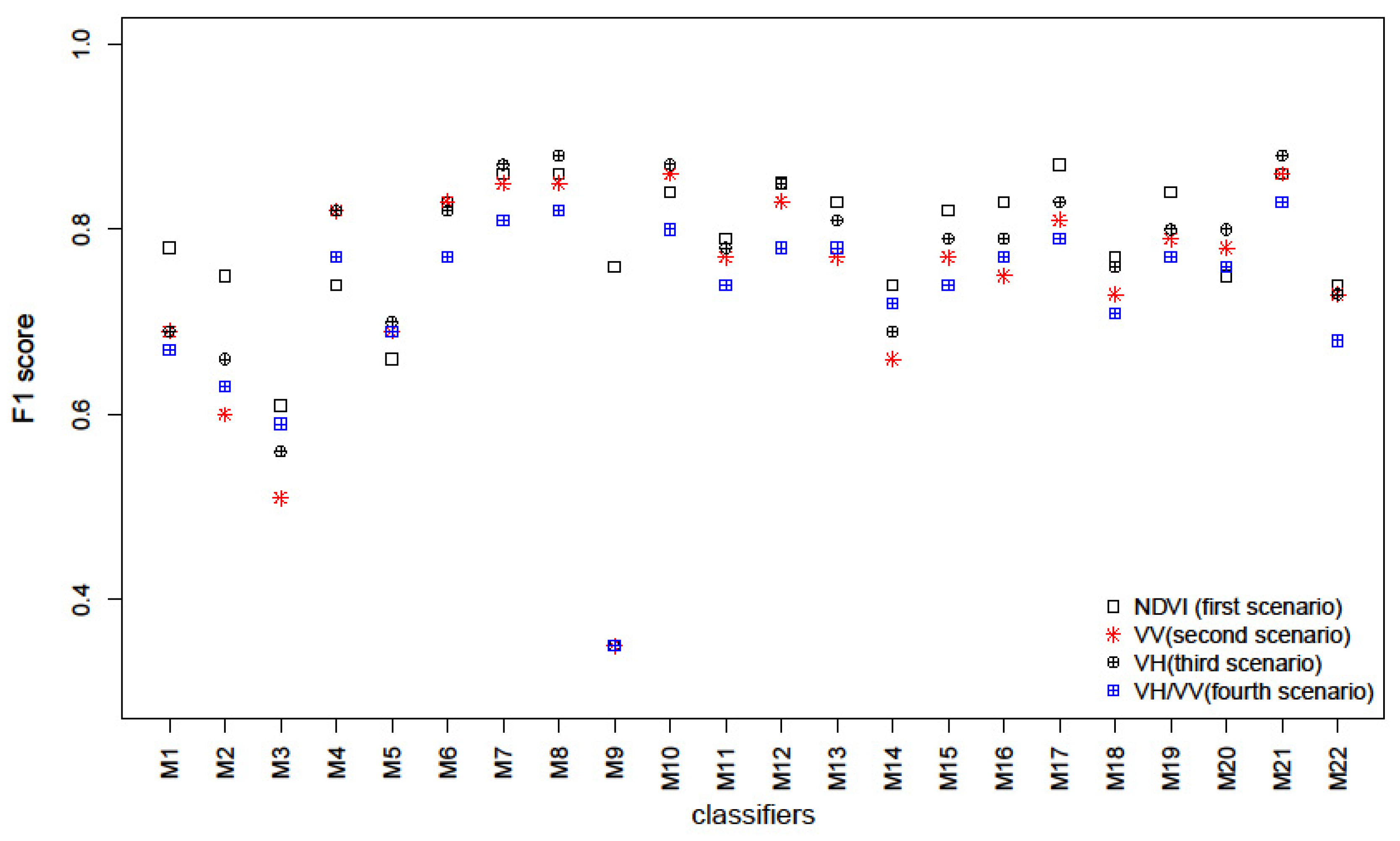
The results of the classification scenarios using only Sentinel-1 information were obtained for the evaluated classification methods and are shown in Figure 8. In this section, we compare the F1 score between the scenarios of the first approach and the reference one (only Sentinel-2 NDVI). In general, VH/VV underperforms compared with NDVI, VV, and VH. Regarding SAR derived information, VH in general presents better performance than VV. Further, when comparing NDVI and VH information, depending on the classification algorithm, one performs better than the other. Decision tree algorithms perform better with NDVI values than with SAR derived information. The same conclusions are obtained with nearest neighbor algorithms. However, the use of support vector machines with VH information in general improves the results of the classification process, leading to the best results for the M8 algorithm. Regarding ensemble classifiers, there are different results depending on the selected algorithm, but the best performing algorithm, M21, slightly improves the classification performance compared to NDVI. Thus, according to our results, SAR derived information for classification can outperform optical information if adequate classification algorithms are selected.
The classification algorithm that obtained the best F1 score in any scenario is the M21 ensemble classifier of type KNN subspace (Table 4). Using SAR data slightly improves the classification results (0.87 over 0.88), mainly when VH polarization is utilized. So, it can be concluded that for M21, crop classification with only optical data or only SAR information performs similarly. This is relevant because the Sentinel-2A mission started in 2015, while Sentinel-1 started in 2014. This makes it possible to perform crop classification from earlier dates, taking advantage of the 10 m resolution of this mission.

3.3. Evaluation of Classification Methods with SAR and Optical Data

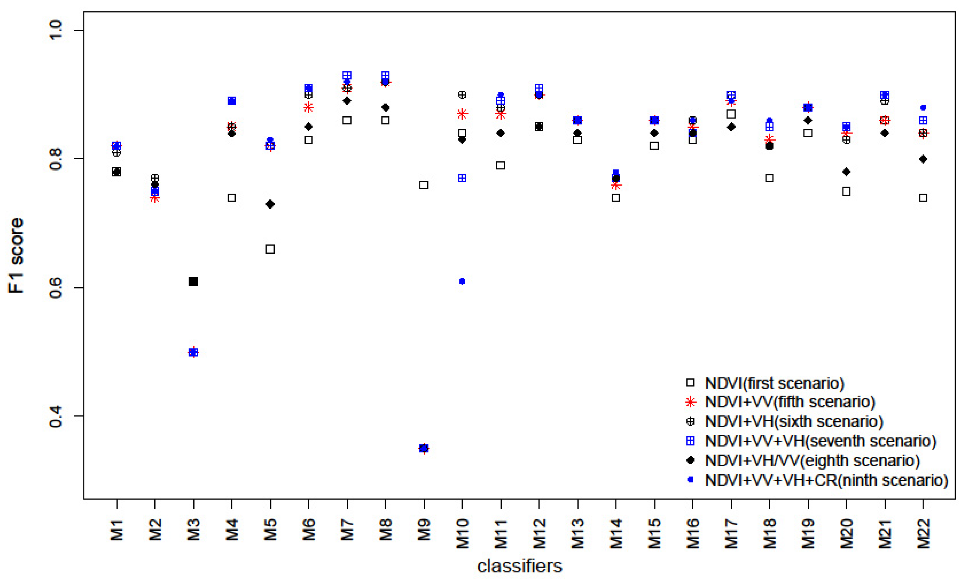
The results of the classification scenarios incorporating Sentinel-1 and Sentinel-2 information were obtained for the 22 algorithms, as shown in Figure 9. In this section, we compare the different scenarios of the second approach and the reference one in order to evaluate the added value that SAR features can bring to classical classification methodology (based on only optical data).
When combining NDVI and VV information, we noticed that for the majority of classifiers this incorporation improved the F1 score results compared to using only NDVI information, except for M3 and M9. The same observation can be made when comparing the scenario using NDVI combined with VH with the one using only NDVI information. Concerning the eighth scenario (VH/VV incorporated with NDVI), for the majority of the classifiers it presented only a slight improvement in F1 score compared to using only NDVI information, except for M1 and M2, which had the same F1 score in both scenarios. Further, the eighth scenario registered the lowest F1 score among all scenarios. Thus, the VH/VV ratio did not contribute to improving the classification results, and for some classifiers it deteriorated the accuracy compared to scenarios incorporating VV or VH with NDVI.
According to our results, it can be inferred that the fifth (NDVI+VV) and sixth (NDVI+VH) scenarios provided, for almost all classifiers, equal or very similar results. Thus, VV and VH contribute equally to improving the classification process. Furthermore, it can be noticed that generally the difference between F1 scores of the fifth (NDVI+VV), sixth (NDVI+VH), seventh (NDVI+VH+VV), and ninth (NDVI+VH+VV+VH/VV) scenarios is very narrow, but it is important to mention that the majority of classifiers presented their best F1 score with the seventh scenario. Therefore, we conclude that using the seventh scenario (NDIV+VV+VH), integrating VH and VV, both, polarization channels with NDVI may offer the best option to improve classification accuracy.
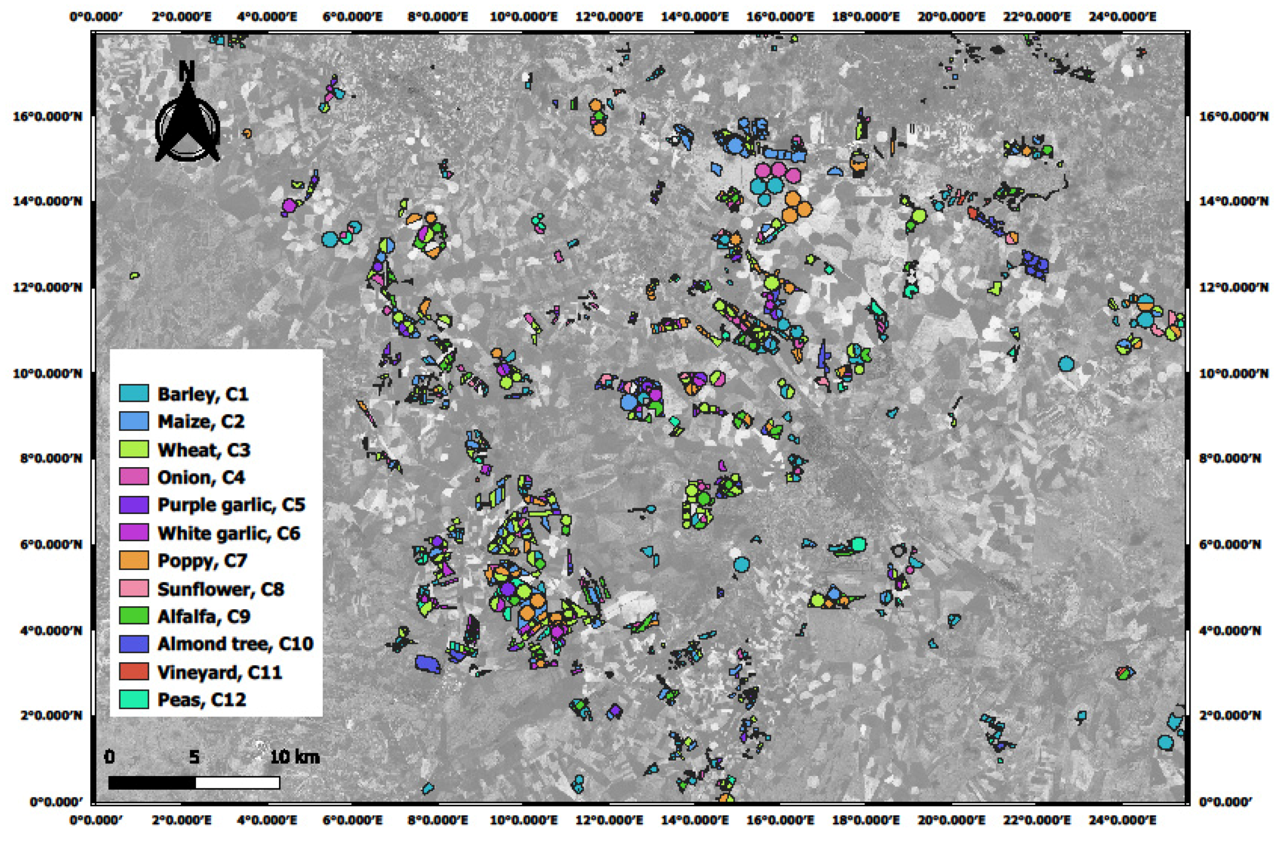
Regarding the algorithm with the best performance for the crop classification task, Table 5 shows that when integrating optical and SAR information, the M8 (cubic SVM) algorithm returns better results than M21. Furthermore, combining optical and SAR information increases the F1 score from 0.87 to 0.93, highlighting the improvement of crop classification with the proposed approach. The classification results obtained with the best classifier M8 when applying the seventh scenario (NDVI+VH+VV) are shown in Figure 10.

3.4. Evaluation of Best Method of Crop Classification with First and Seventh Scenarios

The following section provides a demonstration of the confusion matrix of M8, the best performing classifier, in the seventh scenario (Table 6) and the first one (Table 7) in order to highlight how the incorporation of VH and VV with NDVI improved UA and PA, and to evaluate the misclassified cases.
Our analysis is based on the distribution of crops into groups according to the improvement or deterioration brought by the seventh scenario compared to the first one:
  • First group: barley C1, maize C2, wheat C3, onion C4, purple garlic C5, grapevines C11, and peas C12. For these crops, the seventh scenario improved both UA and PA.
  • Second group: sunflower C8. The seventh scenario improved only UA.
  • Third group: alfalfa C9, and almond tree C10. The seventh scenario improved only PA.
Analyzing the results of the first group, we noticed that the introduction of VH and VV significantly improved UA and PA for peas, barley, wheat, and purple garlic. Indeed, the improvement between the reference and seventh scenarios for UA ranged between 6.1% and 36.7% and for PA ranged between 5.1% and 22.5%.
The second group contained only sunflower C8. UA was improved by 33.4% and PA decreased to 13.3%. The sunflower also had the lowest PA value with the best performing classifier because of the small number of visited plots, which led to worse calibration and validation of the algorithm, this can be the reason for the obtained result for this specific crop type.
Focusing on the third group, concerning alfalfa C9, PA was enhanced by 2.4% and UA deteriorated by 4.5%. Indeed, it was wrongly classified as wheat C3 four times, and one time each as maize C2 and sunflower C8. All this misclassification may be explained by the fact that these crops have coinciding phenological phases. In the case of permanent crops, almond tree C10 the classification results were good although that permanent crops have special temporal signatures because they are predominated essentially by soil backscatter due to the open spaces between trees.

4. Discussion

In this current work, we assessed the potential of integrating Sentinel-1 information (VV and VH backscatter and their ratio VH/VV) with Sentinel-2A data (NDVI) to improve the crop classification and to define which are the most important input data that provide the most accurate classification results. Furthermore, we evaluated the performance of 22 nonparametric classifiers on which most of these algorithms had not been tested before with SAR data.
As a general tendency when using only Sentinel-1 information, the classification performance of the majority of classifiers achieved very similar accuracy with VH and VV polarization channels, while classification using the VH/VV ratio as the input obtained lower accuracy. Similar results were obtained in [36] in which the principal objective was to evaluate the performance of a supervised crop classification approach based on only crop temporal signatures obtained from Sentinel-1 time series without optical data.
According to our classification results, the seventh scenario (NDVI+ VH+VV) is considered the best scenario. Then, the integration of both polarization channel VH and VV with NDVI has improved the classification accuracy, and this can be explained by the fact that radar signals interact differently with land cover components [68], therefore it is important to choose adequate polarization channels that allow the representation of the most important backscatter mechanisms. Indeed, according to [29,69], the VH backscatter is dominated by the attenuated double bounce (when targets and ground surface are perpendicular, they can act as corner reflectors, providing a “double-bounce” scattering effect that sends the radar signals back in the direction they came from) and volume scattering mechanisms (volume scattering occurs when the radar signal is subjected to multiple reflections within three-dimensional matter; at the shorter C-band wavelength, it can take place within the canopy of lower or sparse vegetation types), while the VV backscatter is dominated by direct contributions from the ground and the canopy. Consequently, the integration of both VH and VV allowed the capture of all the important backscatter mechanisms during the phenological cycle of the observed crops. However, looking in the literature, we did not find a consensus about the most pertinent features derived from SAR imagery. In [34] it was found that Haralick texture features (entropy and inertia), the VH/VV ratio, and the local mean together with the VV imagery contain most of the information needed for accurate classification. However, in [36] it was found that the most important features in the classification scheme are VH/VV and Haralick texture. Another study [33] did not find any clear difference in importance between the two polarization channels (VV and VH).
As mentioned previously in the results section, all the results of the tested scenarios in the second approach (when integrating optical and SAR information) show that M8 (cubic SVM) was the best performing classifier and showed better results than M21.In [38] it was concluded that M21 provided the best classification result using optical data (NDVI derived from Sentinel-2 and Landsat-8), and in the present work this classifier showed slight improvement with the seventh scenario, rising from 0.87 to 0.90. Therefore, incorporating SAR information (VV and VH polarization) can only improve the performance of the classifiers; with a non-robust classifier (M4) it generates important improvements and with a robust classifier (M21 and M12) it generates slight improvements. However, even with the best scenario, we notice that M9 and M10presented the worst results. M9 presented an F1 score of 0.35 in all scenarios, but a relatively high F1 score of 0.77 in the first scenario (only NDVI). Based on this observation, we can conclude that probably the M9 classifier, medium Gaussian SVM, is not adequate for classification with SAR data. This conclusion can also be applied to M3.
Additionally, this study compared the performance of the best classifier M8 with the reference (only NDVI as input) and Seventh (NDVI+VH+VV) Scenarios. This comparison revealed that the introduction of VH and VV significantly improved both UA and PA for peas, barley, maize, wheat, and purple and white garlic. Indeed, the improvement between the reference and seventh scenarios for UA ranged between 5.9% and 23.4% and for PA ranged between 7.3% and 12.3%. The resulting enhancement was noted especially for cereals (barley and wheat). This observation can be explained by the fact that cereals have a quite distinctive temporal signature, as found in [67], and as shown in Figure 4. Furthermore, the presence of more clouds in spring could lead to SAR supplying more information for classification. Corn C2 achieved good classification results; both UA and PA were slightly improved despite the temporal signature of VV and VH being distinguished from other crops. In fact, the patterns of VV and VH of corn in our study area were very similar to the pattern described in [70]: VH increased because of volume scattering during the vegetative period until reaching the maximum height, and after that stayed constant, and the VV curve has the general tendency of VH, but its main characteristic is that it is rather higher than the other VV crop curves. Moreover, for peas C12, the improvement of UA and PA in the seventh scenario were very notable, actually they increased by 23.4% and 9.6%, respectively. This may be due to the volume backscatter produced by the heterogeneous shrub-like structure of legume canopies as found in [66].

5. Conclusions

In this paper, we evaluated the performance of 22 nonparametric classifiers with SAR Sentinel-1 and optical Sentinel-2A data employing a simple and efficient methodology that allows the incorporation of dense time-series of datasets (22 Sentinel-2A and 39 Sentinel-1 different acquisition date), so that the phenological temporal dynamics of the studied crops can be completely detected. The simple methodology consisted in computing the mean of the optical feature (NDVI) and SAR feature (VV, VH and VH\VV) at plot level (plot-based approach) for each available date without recourse to the calculation of other feature like Haralick texture features (entropy and inertia). Nine classification scenarios based on the selection of input features were then applied.
The results of the first approach based on the use of only SAR data as the input feature revealed two important conclusions. The First one is that classification results, in general, presented better performance with VH than with VV or with VH\VV. The second one is that SAR-derived information VH can outperform optical information NDVI if adequate classification algorithms are selected (the case of M5, M7, M8, M10, M12, M20, and M21).
The results of the second approach, which is based on integrating SAR with optical data, showed that the best tested scenario was the integration of VH and VV with NDVI. Consequently, we recommend the use of both VH and VV as input features to take advantage of the different information that these two polarization channels can provide. Concerning the tested classifiers, we found that the best performing one was cubic support vector machine SVM (F1 score = 0.93); indeed, with this classifier the F1 score was improved by 6% compared to the results provided by the best performing classifier M21 (F1 score = 0.87) in the reference scenario (the first one). Furthermore, we concluded that some classifiers (M3 and M9) are not adequate to deal with SAR data, except these two classifiers, incorporating SAR information (VV and VH polarization) can only improve the performance of the classifiers; with a non-robust classifier (for example M4) generated important improvements and with a robust classifier (M21 and M12) generated slight improvements.

Author Contributions

Conceptualization, D.H.-L., R.B. and M.A.M.; data curation, A.C.; formal analysis, A.C., D.H.-L., R.B. and M.A.M.; funding acquisition, D.H.-L. and M.A.M.; investigation, A.C. and D.H.-L.; methodology, A.C., D.H.-L., R.B. and M.A.M.; project administration, D.H.-L.; resources, R.B. and M.A.M.; software, A.C., D.H.-L. and M.A.M.; supervision, D.H.-L. and R.B.; visualization, A.C.; writing—original draft, A.C.; writing—review and editing, R.B. and M.A.M. All authors have read and agreed to the published version of the manuscript.

Funding

This research was funded by the Spanish Ministry of Education and Science (MEC), grant number AGL2017-82927-C3-2-R (co-funded by FEDER) and by Junta de Comunidades de Castilla-La Mancha for funding project SBPLY/19/180501/000080.

Institutional Review Board Statement

Not applicable.

Informed Consent Statement

Not applicable.

Data Availability Statement

The data presented in this study are available on request from the corresponding author. The data are not publicly available because the ground truth data belongs to the Confederación Hidrográfica del Júcar, Spain.

Acknowledgments

We would like to acknowledge the support of the Confederación Hidrográfica del Júcar, and the University of Castilla-La Mancha for funding a PhD grant for Amal Chakhar.

Conflicts of Interest

The authors declare no conflict of interest.

References

  1. Liu, P. A survey of remote-sensing big data. Front. Environ. Sci. 2015, 3, 1–6. [Google Scholar] [CrossRef] [Green Version]
  2. Anderson, K.; Ryan, B.; Sonntag, W.; Kavvada, A.; Friedl, L. Earth observation in service of the 2030 Agenda for Sustainable Development. Geo-Spatial Inf. Sci. 2017, 20, 77–96. [Google Scholar] [CrossRef]
  3. Xie, Y.; Sha, Z.; Yu, M. Remote sensing imagery in vegetation mapping: A review. J. Plant. Ecol. 2008, 1, 9–23. [Google Scholar] [CrossRef]
  4. Hall, A.; Lamb, D.W.; Holzapfel, B.; Louis, J. Hall, Lamb, Holzapfel & Louis. Aust. J. Grape Wine Res. 2002, 8, 36–47. [Google Scholar]
  5. Behzad, A.; Aamir, M.; Raza, S.A.; Qaiser, A.; Fatima, S.Y.; Karamat, A.; Mahmood, S.A. Estimation of Wheat Area using Sentinel-1 and Sentinel-2 Datasets (A Comparative Analysis). Int. J. Agric. Sustain. Dev. 2019, 1, 81–93. [Google Scholar] [CrossRef]
  6. Wolanin, A.; Camps-Valls, G.; Gómez-Chova, L.; Mateo-García, G.; Van Der Tol, C.; Zhang, Y.; Guanter, L. Estimating crop primary productivity with Sentinel-2 and Landsat 8 using machine learning methods trained with radiative transfer simulations. Remote Sens. Environ. 2019, 225, 441–457. [Google Scholar] [CrossRef]
  7. Lambert, M.J.; Traoré, P.C.S.; Blaes, X.; Baret, P.; Defourny, P. Estimating smallholder crops production at village level from Sentinel-2 time series in Mali’s cotton belt. Remote Sens. Environ. 2018, 216, 647–657. [Google Scholar] [CrossRef]
  8. Awad, M.M. Toward precision in crop yield estimation using remote sensing and optimization techniques. Agriculture 2019, 9, 54. [Google Scholar] [CrossRef] [Green Version]
  9. Tan, S.; Wu, B.; Yan, N.; Zeng, H. Satellite-based water consumption dynamics monitoring in an extremely arid area. Remote Sens. 2018, 10, 1399. [Google Scholar] [CrossRef] [Green Version]
  10. Wu, X.; Zhou, J.; Wang, H.; Li, Y.; Zhong, B. Evaluation of irrigation water use efficiency using remote sensing in the middle reach of the Heihe river, in the semi-arid Northwestern China. Hydrol. Process. 2015, 29, 2243–2257. [Google Scholar] [CrossRef]
  11. Löw, F.; Michel, U.; Dech, S.; Conrad, C. Impact of feature selection on the accuracy and spatial uncertainty of per-field crop classification using Support Vector Machines. ISPRS J. Photogramm. Remote Sens. 2013, 85, 102–119. [Google Scholar] [CrossRef]
  12. Liu, C.A.; Chen, Z.X.; Shao, Y.; Chen, J.S.; Hasi, T.; Pan, H.Z. Research advances of SAR remote sensing for agriculture applications: A review. J. Integr. Agric. 2019, 18, 506–525. [Google Scholar] [CrossRef] [Green Version]
  13. Tucker, C.J.; Holben, B.N.; Elgin, J.H.; McMurtrey, J.E. Relationship of spectral data to grain yield variation. Photogramm. Eng. Remote Sens. 1980, 46, 657–666. [Google Scholar]
  14. Wang, K.; Franklin, S.E.; Guo, X.; He, Y.; McDermid, G.J. Problems in remote sensing of landscapes and habitats. Prog. Phys. Geogr. 2009, 33, 747–768. [Google Scholar] [CrossRef] [Green Version]
  15. Feingersh, T.; Gorte, B.G.H.; Van Leeuwen, H.J.C. Fusion of SAR and SPOT image data for crop mapping. Int. Geosci. Remote Sens. Symp. 2001, 2, 873–875. [Google Scholar] [CrossRef]
  16. Patel, P.; Srivastava, H.S.; Panigrahy, S.; Parihar, J.S. Comparative evaluation of the sensitivity of multi-polarized multi-frequency SAR backscatter to plant density. Int. J. Remote Sens. 2006, 27, 293–305. [Google Scholar] [CrossRef]
  17. Wempen, J.M.; McCarter, M.K. Comparison of L-band and X-band differential interferometric synthetic aperture radar for mine subsidence monitoring in central Utah. Int. J. Min. Sci. Technol. 2017, 27, 159–163. [Google Scholar] [CrossRef]
  18. Dobson, M.C.; Ulaby, F. Microwave Backscatter Dependence on Surface Roughness, Soil Moisture, and Soil Texture: Part III—Soil Tension. IEEE Trans. Geosci. Remote Sens. 1981, GE-19, 51–61. [Google Scholar] [CrossRef]
  19. Ulaby, F.T.; Moore, R.K.; Fung, A.K. Microwave remote sensing fundamentals and radiometry. In Microwave Remote Sensing: Active and Passive; Artech House: Boston, MA, USA, 1981; Volume 1. [Google Scholar]
  20. Baghdadi, N.; Gherboudj, I.; Zribi, M.; Sahebi, M.; King, C. Semi-empirical calibration of the IEM backscattering model using radar images and moisture and roughness field measurements. Int. J. Remote Sens. 2004, 37–41. [Google Scholar] [CrossRef]
  21. Ulaby, F.T.; Razani, M.; Dobson, M.C. Effects of Vegetation Cover on the Microwave Radiometric Sensitivity to Soil Moisture. IEEE Trans. Geosci. Remote Sens. 1983, GE-21, 51–61. [Google Scholar] [CrossRef]
  22. Hallikainen, M.T.; Ulaby, F.T.; Dobson, M.C.; El-Rayes, M.A.; Wu, L.-K. Microwave Dielectric Behavior of Wet Soil-Part I: Empirical models. IEEE Trans. Geosci. Remote Sens. 1985, GE-23, 25–34. [Google Scholar] [CrossRef]
  23. Oh, Y.; Sarabandi, K.; Ulaby, F.T. An empirical model and an inversion technique for radar scattering from bare soil surfaces. IEEE Trans. Geosci. Remote Sens. 1992, 30, 370–381. [Google Scholar] [CrossRef]
  24. Haris, M.; Ashraf, M.; Ahsan, F.; Athar, A.; Malik, M. Analysis of SAR images speckle reduction techniques. In Proceedings of the International Conference on Computing, Mathematics and Engineering Technologies (iCoMET), Sukkur, Pakistan, 3−4 March 2018; pp. 1–7. [Google Scholar] [CrossRef]
  25. Argenti, F.; Lapini, A.; Alparone, L.; Bianchi, T. A tutorial on speckle reduction in synthetic aperture radar images. IEEE Geosci. Remote Sens. Mag. 2013, 1, 6–35. [Google Scholar] [CrossRef] [Green Version]
  26. Joshi, N.; Baumann, M.; Ehammer, A.; Fensholt, R.; Grogan, K.; Hostert, P.; Jepsen, M.R.; Kuemmerle, T.; Meyfroidt, P.; Mitchard, E.T.A.; et al. A review of the application of optical and radar remote sensing data fusion to land use mapping and monitoring. Remote Sens. 2016, 8, 70. [Google Scholar] [CrossRef] [Green Version]
  27. Ulaby, F.T.; Long, D.G. Microwave Radar and Radiometric Remote Sensing; The University of Michigan Press: Ann Arbor, MI, USA, 2014; ISBN 978-0-472-11935-6. [Google Scholar]
  28. Stendardi, L.; Karlsen, S.R.; Niedrist, G.; Gerdol, R.; Zebisch, M.; Rossi, M.; Notarnicola, C. Exploiting time series of Sentinel-1 and Sentinel-2 imagery to detect meadow phenology in mountain regions. Remote Sens. 2019, 11, 542. [Google Scholar] [CrossRef] [Green Version]
  29. Veloso, A.; Mermoz, S.; Bouvet, A.; Toan, T.L.; Planells, M.; Dejoux, J.; Ceschia, E. Understanding the temporal behavior of crops using Sentinel-1 and Sentinel-2-like data for agricultural applications. Remote Sens. Environ. 2017, 199, 415–426. [Google Scholar] [CrossRef]
  30. Orynbaikyzy, A.; Gessner, U.; Mack, B.; Conrad, C. Crop type classification using fusion of sentinel-1 and sentinel-2 data: Assessing the impact of feature selection, optical data availability, and parcel sizes on the accuracies. Remote Sens. 2020, 12, 2779. [Google Scholar] [CrossRef]
  31. Gao, H.; Wang, C.; Wang, G.; Zhu, J.; Tang, Y.; Shen, P.; Zhu, Z. A crop classification method integrating GF-3 PolSAR and sentinel-2A optical data in the Dongting lake basin. Sensors 2018, 18, 3139. [Google Scholar] [CrossRef] [Green Version]
  32. Kussul, N.; Mykola, L.; Shelestov, A.; Skakun, S. Crop inventory at regional scale in Ukraine: Developing in season and end of season crop maps with multi-temporal optical and SAR satellite imagery. Eur. J. Remote Sens. 2018, 51, 627–636. [Google Scholar] [CrossRef] [Green Version]
  33. Van Tricht, K.; Gobin, A.; Gilliams, S.; Piccard, I. Synergistic use of radar sentinel-1 and optical sentinel-2 imagery for crop mapping: A case study for Belgium. Remote Sens. 2018, 10, 1642. [Google Scholar] [CrossRef] [Green Version]
  34. Inglada, J.; Vincent, A.; Arias, M.; Marais-Sicre, C. Improved Early Crop Type Identification By Joint Use of High Temporal Resolution SAR And Optical Image Time Series. Remote Sens. 2016, 8, 362. [Google Scholar] [CrossRef] [Green Version]
  35. Inglada, J.; Arias, M.; Tardy, B.; Hagolle, O.; Valero, S.; Morin, D.; Dedieu, G.; Sepulcre, G.; Bontemps, S.; Defourny, P.; et al. Assessment of an operational system for crop type map production using high temporal and spatial resolution satellite optical imagery. Remote Sens. 2015, 7, 12356–12379. [Google Scholar] [CrossRef] [Green Version]
  36. Demarez, V.; Helen, F.; Marais-Sicre, C.; Baup, F. In-season mapping of irrigated crops using Landsat 8 and Sentinel-1 time series. Remote Sens. 2019, 11, 118. [Google Scholar] [CrossRef] [Green Version]
  37. Sun, Y.; Luo, J.; Wu, T.; Zhou, Y.N.; Liu, H.; Gao, L.; Dong, W.; Liu, W.; Yang, Y.; Hu, X.; et al. Synchronous response analysis of features for remote sensing crop classification based on optical and SAR time-series data. Sensor 2019, 19, 4227. [Google Scholar] [CrossRef] [PubMed] [Green Version]
  38. Chakhar, A.; Ortega-Terol, D.; Hernández-López, D.; Ballesteros, R.; Ortega, J.F.; Moreno, M.A. Assessing the Accuracy of Multiple Classification Algorithms for Crop Classification Using Landsat-8. Remote Sens. 2020, 12, 1735. [Google Scholar] [CrossRef]
  39. Hao, P.Y.; Tang, H.J.; Chen, Z.X.; Yu, L.; Wu, M.Q. High resolution crop intensity mapping using harmonized Landsat-8 and Sentinel-2 data. J. Integr. Agric. 2019, 18, 2883–2897. [Google Scholar] [CrossRef]
  40. Orynbaikyzy, A.; Gessner, U.; Conrad, C. Crop type classification using a combination of optical and radar remote sensing data: A review. Int. J. Remote Sens. 2019, 40, 6553–6595. [Google Scholar] [CrossRef]
  41. Kobayashi, N.; Tani, H.; Wang, X.; Sonobe, R. Crop classification using spectral indices derived from Sentinel-2A imagery. J. Inf. Telecommun. 2019, 4, 67–90. [Google Scholar] [CrossRef]
  42. Htitiou, A.; Boudhar, A.; Lebrini, Y.; Hadria, R.; Lionboui, H.; Elmansouri, L.; Tychon, B.; Benabdelouahab, T. The Performance of Random Forest Classification Based on Phenological Metrics Derived from Sentinel-2 and Landsat 8 to Map Crop Cover in an Irrigated Semi-arid Region. Remote Sens. Earth Syst. Sci. 2019, 2, 208–224. [Google Scholar] [CrossRef]
  43. Nguyen, M.D.; Baez-Villanueva, O.M.; Bui, D.D.; Nguyen, P.T.; Ribbe, L. Harmonization of Landsat and Sentinel 2 for Crop Monitoring in Drought Prone Areas: Case Studies of NinhThuan (Vietnam) and Bekaa (Lebanon). Remote Sens. 2020, 12, 281. [Google Scholar] [CrossRef] [Green Version]
  44. Blaes, X.; Defourny, P.; Wegmüller, U.; Member, S.; Della Vecchia, A.; Guerriero, L.; Ferrazzoli, P.; Member, S. C-Band Polarimetric Indexes for Maize Monitoring Based on a Validated Radiative Transfer Model. IEEE Trans. Geosci. Remote Sens. 2006, 44, 791–800. [Google Scholar] [CrossRef]
  45. Filipponi, F. Sentinel-1 GRD Preprocessing Workflow. Proceedings 2019, 18, 11. [Google Scholar] [CrossRef] [Green Version]
  46. Kaplan, G. Monthly Analysis of Wetlands Dynamics Using Remote Sensing Data. Int. J. GeoInf. Artic. 2018, 7, 411. [Google Scholar] [CrossRef] [Green Version]
  47. Sentinel-1 Product Specification.Ref. S1-RS-MDA-52-7440; MacDonald, Dettwiler Assoc. Ltd.: Richmond, BC, Canada, 2011.
  48. Filgueiras, R.; Mantovani, E.C.; Altho, D. Crop NDVI Monitoring Based on Sentinel 1. Remote Sens. 2019, 11, 1441. [Google Scholar] [CrossRef] [Green Version]
  49. Yommy, A.S.; Liu, R.; Wu, A.S. SAR Image despeckling using refined Lee filter. In Proceedings of the 7th International Conference on Intelligent Human-Machine Systems and Cybernetics, Hangzhou, China, 26–27 August 2015; pp. 260–265. [Google Scholar]
  50. Breiman, L.; Friedman, J.H.; Olshen, R.A.; Stone, C.J. Classification and Regression Trees, 1st ed.; Routledge: Boca Raton, FL, USA, 1984; ISBN 9781351460491. [Google Scholar]
  51. Champagne, C.; McNairn, H.; Daneshfar, B.; Shang, J. A bootstrap method for assessing classification accuracy and confidence for agricultural land use mapping in Canada. Int. J. Appl. Earth Obs. Geoinf. 2014, 29, 44–52. [Google Scholar] [CrossRef] [Green Version]
  52. Douglas, F.; Pat, L.; Fisher, R. Methods of Conceptual Clustering and their Relation to Numerical Taxonomy. Ann. Eugen. 1985, 7, 179–188. [Google Scholar]
  53. Cristianini, N.; Shawe-Taylor, J. An Introduction to Support. Vector Machines and Other Kernel-based Learning Methods; Cambridge University Press: Cambridge, UK, 2000; ISBN 9780511801389. [Google Scholar]
  54. Nadkarni, P. Core Technologies: Data Mining and “Big Data”. Clin. Res. Comput. 2016, 9, 187–204. [Google Scholar]
  55. Breiman, L. Stacked regressions. Mach. Learn. 1996, 24, 49–64. [Google Scholar] [CrossRef] [Green Version]
  56. Hansen, L.K.; Salamon, P. Neural Network Ensembles. IEEE Trans. Pattern Anal. Mach. Intell. 1990, 12, 993–1001. [Google Scholar] [CrossRef] [Green Version]
  57. Breiman, L. Bagging predictors. Mach. Learn. 1996, 24, 123–140. [Google Scholar] [CrossRef] [Green Version]
  58. Schapire, R.E.; Freund, Y.; Bartlett, P.; Lee, W.S. Boosting the margin: A new explanation for the effectiveness of voting methods. Ann. Stat. 1998, 26, 1651–1686. [Google Scholar] [CrossRef]
  59. Congalton, R.G. A review of assessing the accuracy of classifications of remotely sensed data. Remote Sens. Environ. 1991, 37, 35–46. [Google Scholar] [CrossRef]
  60. Pedregosa, F.; Varoquaux, G.; Gramfort, A.; Michel, V.; Thirion, B.; Grisel, O.; Blondel, M.; Prettenhofer, P.; Weiss, R.; Dubourg, V.; et al. Scikit-learn: Machine Learning in Python. J. Mach. Learn. Res. 2011, 12, 2825–2830. [Google Scholar]
  61. Khabbazan, S.; Vermunt, P.; Steele-Dunne, S.; Arntz, L.R.; Marinetti, C.; van der Valk, D.; Iannini, L.; Molijn, R.; Westerdijk, K.; van der Sande, C. Crop monitoring using Sentinel-1 data: A case study from The Netherlands. Remote Sens. 2019, 11, 1887. [Google Scholar] [CrossRef] [Green Version]
  62. Liu, C.; Shang, J.; Vachon, P.W.; McNairn, H. Multiyear crop monitoring using polarimetric RADARSAT-2 data. IEEE Trans. Geosci. Remote Sens. 2013, 51, 2227–2240. [Google Scholar] [CrossRef]
  63. Vreugdenhil, M.; Wagner, W.; Bauer-marschallinger, B.; Pfeil, I.; Teubner, I.; Rüdiger, C.; Strauss, P. Sensitivity of Sentinel-1 Backscatter to Vegetation Dynamics: An Austrian Case Study. Remote Sens. 2018, 10, 1396. [Google Scholar] [CrossRef] [Green Version]
  64. Mattia, F.; Le Toan, T.; Picard, G.; Posa, F.I.; Alessio, A.D.; Notarnicola, C.; Gatti, A.M.; Rinaldi, M.; Satalino, G. Multitemporal C-Band Radar Measurements on Wheat Fields. IEEE Trans. Geosci. Remote Sens. 2003, 41, 1551–1560. [Google Scholar] [CrossRef]
  65. Larranaga, A.; Alvarez-Mozos, J.; Albizua, L.; Peters, J. Backscattering behavior of rain-fed crops along the growing season. IEEE Geosci. Remote Sens. Lett. 2013, 10, 386–390. [Google Scholar] [CrossRef]
  66. Skriver, H.; Svendsen, M.T.; Thomsen, A.G. Multitemporal C- and L-band polarimetric signatures of crops. IEEE Trans. Geosci. Remote Sens. 1999, 37, 2413–2429. [Google Scholar] [CrossRef]
  67. Arias, M.; Campo-Bescós, M.Á.; Álvarez-Mozos, J. Crop classification based on temporal signatures of Sentinel-1 observations over Navarre province, Spain. Remote Sens. 2020, 12, 278. [Google Scholar] [CrossRef] [Green Version]
  68. Alonso-González, A.; Hajnsek, I. Radar remote sensing of land surface parameters. In Observation and Measurement of Ecohydrological Processes, Ecohydrology; Li, X., Vereecken, H., Eds.; Springer: Berlin, Germany, 2019; ISBN 9783662478714. [Google Scholar]
  69. Brown, S.C.M.; Quegan, S.; Morrison, K.; Bennett, J.C.; Cookmartin, G. High-resolution measurements of scattering in wheat canopies—Implications for crop parameter retrieval. IEEE Trans. Geosci. Remote Sens. 2003, 41, 1602–1610. [Google Scholar] [CrossRef] [Green Version]
  70. Bériaux, E.; Waldner, F.; Collienne, F.; Bogaert, P.; Defourny, P. Maize Leaf Area Index retrieval from synthetic quad pol SAR time series using the water cloud model. Remote Sens. 2015, 7, 16204–16225. [Google Scholar] [CrossRef] [Green Version]
Figure 1. Locations of the reference data.
Remotesensing 13 00243 g001
Figure 2. Acquisition dates of Sentinel-2A and Sentinel-1 data.
Remotesensing 13 00243 g002
Figure 3. A zoomed normalized difference vegetation index (NDVI) scene composed by three Sentinel-2A tiles SXJ, SWJ, and SWH (obtained in 2016.03.05) over the study area.
Remotesensing 13 00243 g003
Figure 4. General workflow.
Remotesensing 13 00243 g004
Figure 5. Temporal signatures of maize, barley, and grapevines for Normalized Difference Vegetation Index (NDVI), cross ratio (CR), VH, and VV. Two relative descendant (des) and ascendant (asc) orbits are represented in blue and black, respectively.
Remotesensing 13 00243 g005
Figure 6. Temporal signatures of purple garlic, poppy, and peas for NDVI, CR, VH, and VV. Two relative descendant (des) and ascendant (asc) orbits are represented in black and blue, respectively.
Remotesensing 13 00243 g006
Figure 7. Growing cycles of studied crops for the case study.
Remotesensing 13 00243 g007
Figure 8. F1 score statistics of classification methods of the first approach.
Remotesensing 13 00243 g008
Figure 9. F1 score statistics of classification methods of the second approach.
Remotesensing 13 00243 g009
Figure 10. Visualization of the classification results with the M8 classifier within the seventh scenario.
Remotesensing 13 00243 g010
Table 1. Input data of the scenarios of the first approach.
ScenarioInput Data
Second scenarioonly VV channel
Third scenarioonly VH channel
Fourth scenarioonly VH/VV
Table 2. Input data of the scenarios of the second approach.
ScenarioInput Data
Fifth scenarioNDVI and VV channel
Sixth scenarioNDVI and VH channel
Seventh scenarioNDVI, VV and VH channels.
Eighth scenarioNDVI and VH/VV
Ninth scenarioNDVI, VV, VH, and VH/VV
Table 3. Evaluated classifiers.
GroupAbbreviationMethod
Decision treesM1Complex Tree
M2Medium Tree
M3Simple Tree
Discriminant analysisM4Linear discriminant
M5Quadratic discriminant
Support Vector Machine (SVM)M6Linear SVM
M7Quadratic SVM
M8Cubic SVM
M9Fine Gaussian SVM
M10Medium Gaussian SVM
M11Coarse Gaussian SVM
Nearest Neighbour (KNN)M12Fine KNN
M13Medium KNN
M14Coarse KNN
M15Cosine KNN
M16Cubic KNN
M17Weighted KNN
Ensemble classifiersM18Boosted Trees
M19Bagged Trees
M20Subspace Discriminant
M21Subspace KNN
M22RUS Boost Trees
Table 4. Best performing algorithms in the first approach for each scenario and their F1 scores.
ScenarioBest AlgorithmsF1 Score
NDVI (first scenario)M17, M210.87
VV (second scenario)M10, M210.86
VH (third scenario)M8, M210.88
VH/VV (fourth scenario)M210.83
Table 5. Best performing algorithms in the second approach for each scenario and their F1 score.
ScenarioBest AlgorithmF1 Score
NDVI (first scenario)M17, M210.87
NDVI+VV (fifth scenario)M80.92
NDVI+VH (sixth scenario)M80.92
NDVI+VV+VH (seventh scenario)M80.93
NDVI+VH/VV (eighth scenario)M70.89
NDVI+VV+VH+VH/VV (ninth scenario)M7, M80.92
Table 6. Confusion matrix of the best performing classifier, M8, in the best scenario, NDVI+VV+VH (seventh scenario).
Reference Data
C1C2C3C4C5C6C7C8C9C10C11C12TotalUA* Modification of UA (%)
C11200510002000213092.36.1
C207301000000007498.61.3
C35011100001000211993.311.8
C400035001001013892.12.6
C500002810000002996.613.8
C600001280000013093.30
C700000037000013897.4−2.6
C81000000801201266.733.4
C901400001380004486.4−4.5
C1000000000029203193.50
C1100110000023503989.72.5
C1210000000000293096.736.7
Total12774121382929381238333936
PA94.598.691.792.196.696.697.466.7100.087.989.780.6
* Modification of PA (%)15.11.35.19.210.90−2.6−13.32.47.30.222.5
* Modification of user’s accuracy (UA) and producer’s accuracy (PA; %) were calculated with respect to UA and PA of the confusion matrix of M8 in the first scenario.
Table 7. Confusion matrix of M8 with only NDVI information (first scenario).
Reference Data
C1C2C3C4C5C6C7C8C9C10C11C12TotalUA
C111201001000000713086.2
C207202000000007497.3
C31809701000100211981.5
C400034100100113889.5
C510002410000032982.8
C610001280000003093.3
C7000000380000038100.0
C81103000402101233.3
C911200000400004490.9
C1000000000029203193.5
C1110000000043403987.2
C1260320000010183060.0
Total1417411241282938541363831
PA79.497.386.682.985.796.6100.080.097.680.689.558.1
Publisher’s Note: MDPI stays neutral with regard to jurisdictional claims in published maps and institutional affiliations.

