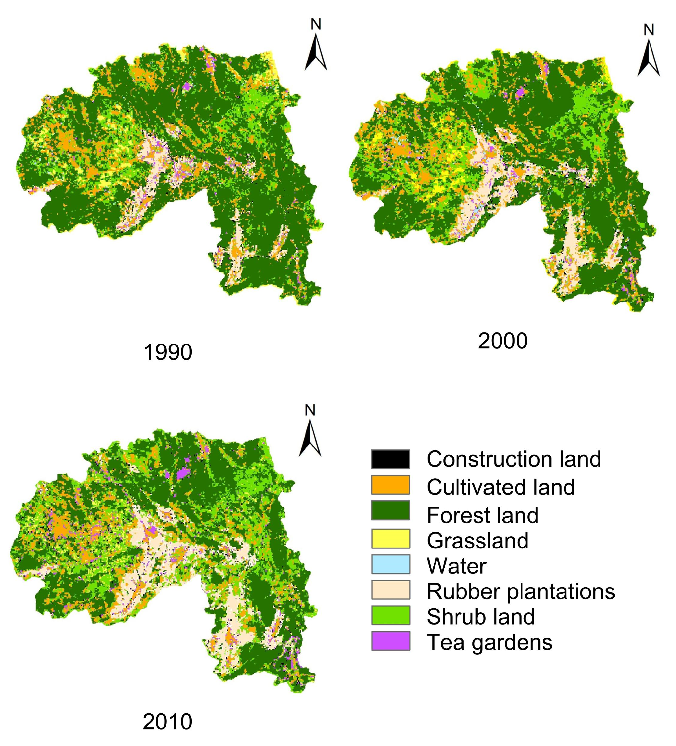
3.1. Analysis of Historical Land Use
The land use maps in 1990, 2000, and 2010 and the accuracies are shown in
Figure 2 and
Appendix A. Firstly we randomly generated 2866, 2549, and 2481 sample points in 1990, 2000, and 2010 through hierarchical random sampling method. There were 1520 sample points, 1227 sample points, and 1008 sample points in forest area in 1990, 2000, and 2010, respectively. Then we evaluated the accuracy of classification for sample points based on Google earth.
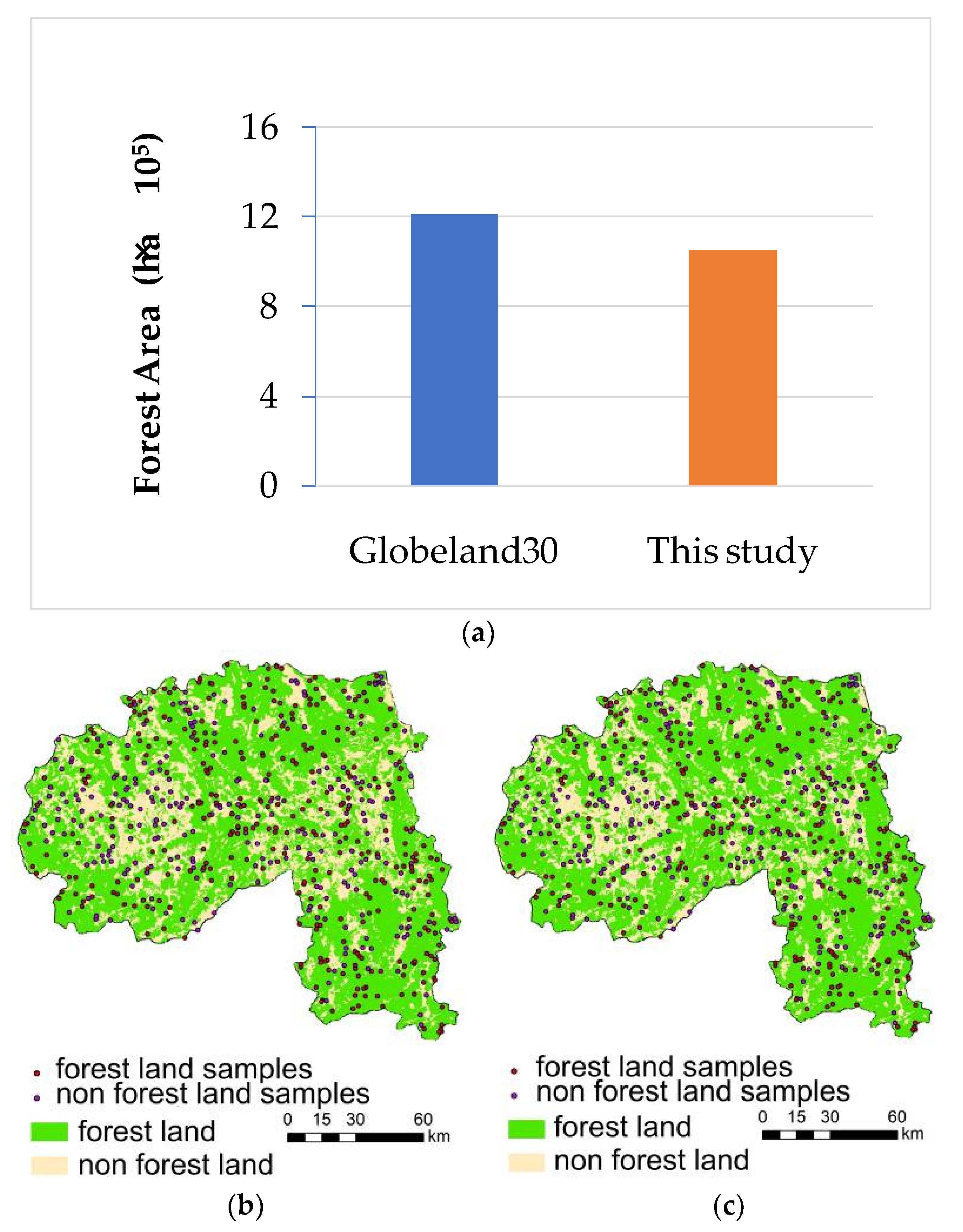
GlobeLand30, which was developed by the National Geomatics Center of China, is an open-access 30m resolution global land cover data product with an overall classification accuracy of over 80% [
62,
63]. We compared the area and spatial location of the forest land in 2010 extracted by Globeland30 with those in this study (
Figure 3). Firstly, about 600 sample points are randomly generated within Xishuangbanna administrative region. Then these sample points are overlapped with Globeland30 and land use map respectively. Finally we evaluate the accuracy of land use map based on the consistency of forest land and nonforest land in Globeland30.
In terms of the forest land area, the forest land area extracted from Globeland30 was 1.21× 10⁶ ha, and that from this study is 1.05×10⁶ ha, with the accuracy 86.92%. In terms of spatial location of the forest land, among 600 randomly generated sample points, 376 were the forest land and 230 were nonforest land in Globeland30; in comparison, 331 sample points were the forest land and 275 sample points were nonforest land in this study. The overall accuracy is 83.66%, and the kappa coefficient is 0.657.
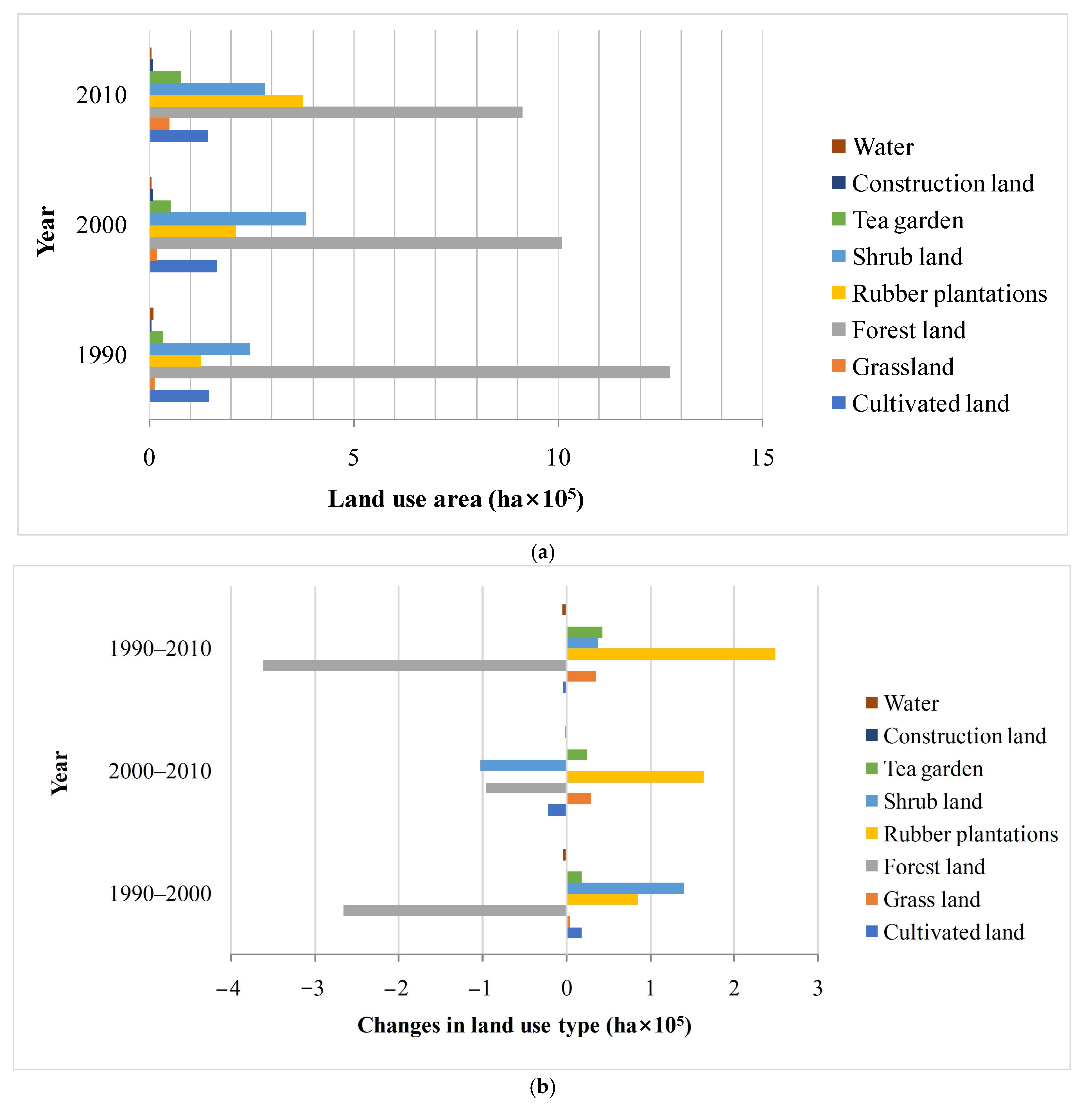
The areas, changes, and dynamics of the three types of land use in 1990, 2000, and 2010 are shown in
Figure 4.
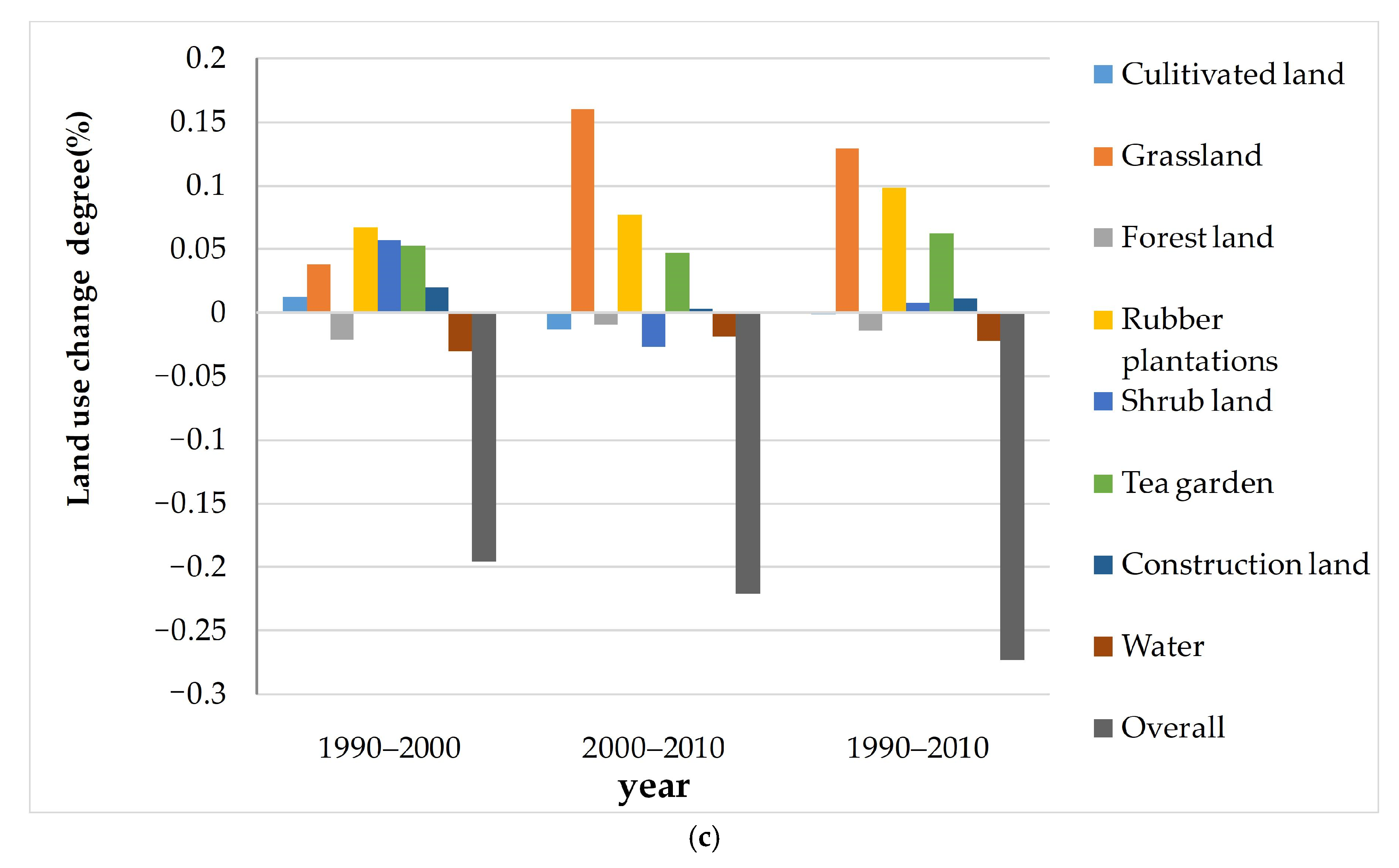
As shown in
Figure 4, the areas under cultivated land, forested land, and water bodies in Xishuangbanna showed a downward trend from 1990 to 2010. Among them, the decrease in forest area is the most obvious, with a total reduction of 360,819 ha (360,819 × 10
4 m
2) over the past 20 years, a dynamic land use change degree of −1.42%, a decrease of 265,491 ha (265,491 × 10
4 m
2) from 1990 to 2000, and a reduction of 95,328 ha (95,328 × 10
4 m
2) from 2000 to 2010. The area of cultivated land showed an increasing trend in the previous 10 years, marked by a rise of 18,153 ha (18,153 × 10
4 m
2) and a dynamic land use change degree of 1.24%. The area of cultivated land decreased by a total of 21,456 ha (21,456 × 10
4 m
2) in the latter 10 years, with a dynamic land use change degree of −1.31%. The area under water bodies declined continuously for the two decades, with a total reduction of 3996 ha (3996 × 10
4 m
2) and a dynamic degree of −2.17%. Grasslands, rubber plantations, shrubland, tea gardens, and construction land in Xishuangbanna region showed increasing trends from 1990 to 2010. Among them, the area of rubber plantations showed the most obvious growth, with a total increase of 249,948 ha (249,948 × 10
4 m
2) in 20 years, and a dynamic land use change degree of 9.87%. Moreover, the area under tea gardens increased by 43,686 ha (43,686 × 10
4 m
2) in the past 20 years, the dynamic land use change degree being 6.26%. Although the areas under grassland, shrubland, and construction land increased, the changes were relatively insignificant.
In summary, the economic development of the Xishuangbanna region and the improvement in people’s quality of life led to a rise in the cultivation of cash crops such as rubber and tea in the region in the past 20 years, resulting in a large number of forests being felled.
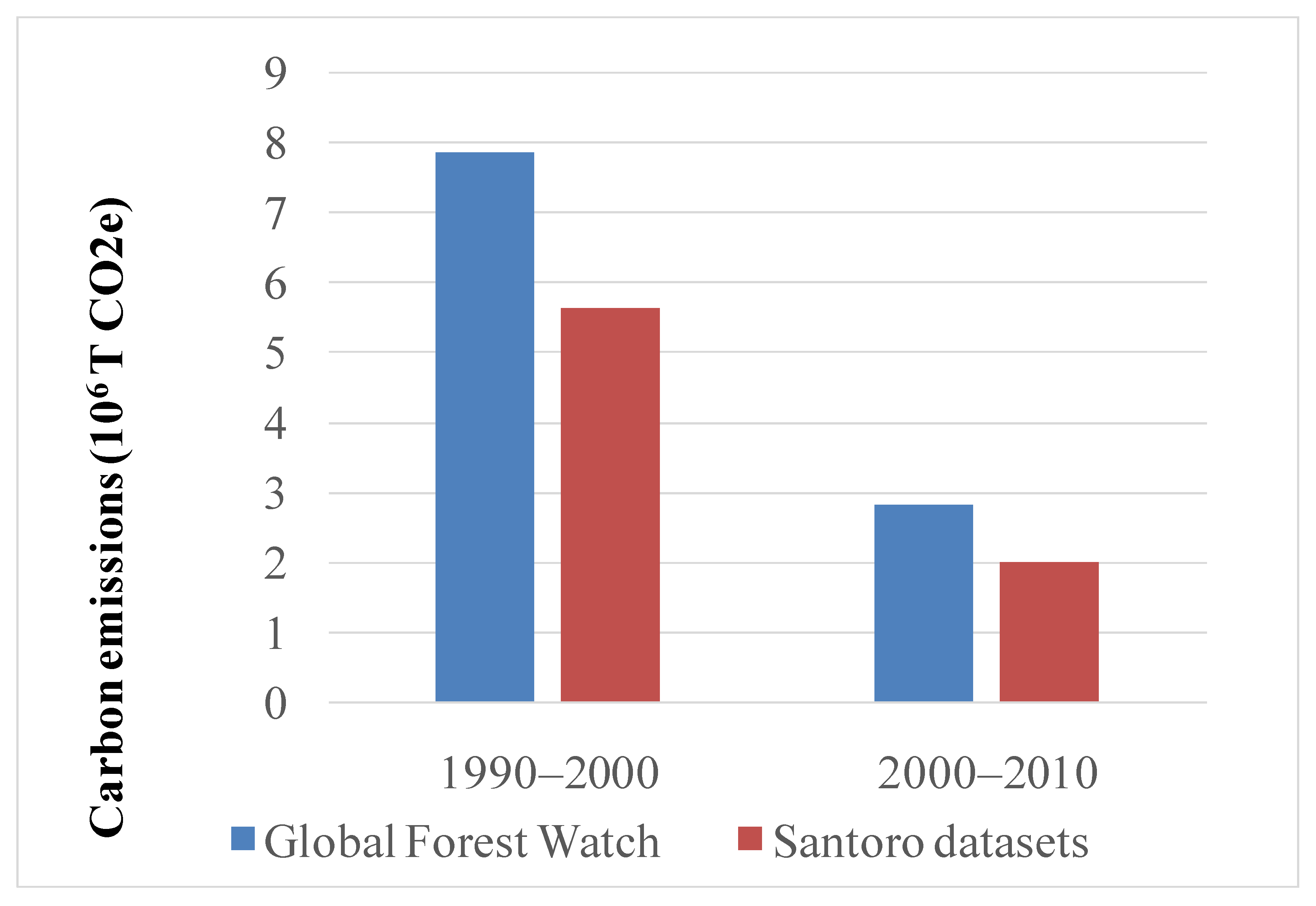
During the period 1990–2000, carbon emissions for Global Forest Watch and Santoro datasets were 7.85 million t CO
2e and 5.63 million t CO
2e, respectively, with a difference of 28.30%. During the period 2000–2010, carbon emissions for Global Forest watch and Santoro datasets were 2.82 million t CO
2e and 2.00 million t CO
2e, respectively, with a difference of 28.81%. Carbon emissions for the period 1990–2000 were about 2.8 times as much as those for the period 2000–2010 (
Figure 5).
3.2. Influencing Factors of Land Use Change
There are many drivers that lead to deforestation and forest degradation within REDD+. Direct drivers are human activities or immediate actions that directly impact forest cover and loss of carbon such as agriculture expansion (both commercial and subsistence), infrastructure extension, and wood extraction. Indirect drivers are complex interactions of social, economic, political, cultural, and technological processes to cause deforestation or forest degradation. They act at multiple scales: international (markets, commodity prices), national (population growth, domestic markets, national policies, governance), and local circumstances (subsistence, poverty) [
64,
65,
66,
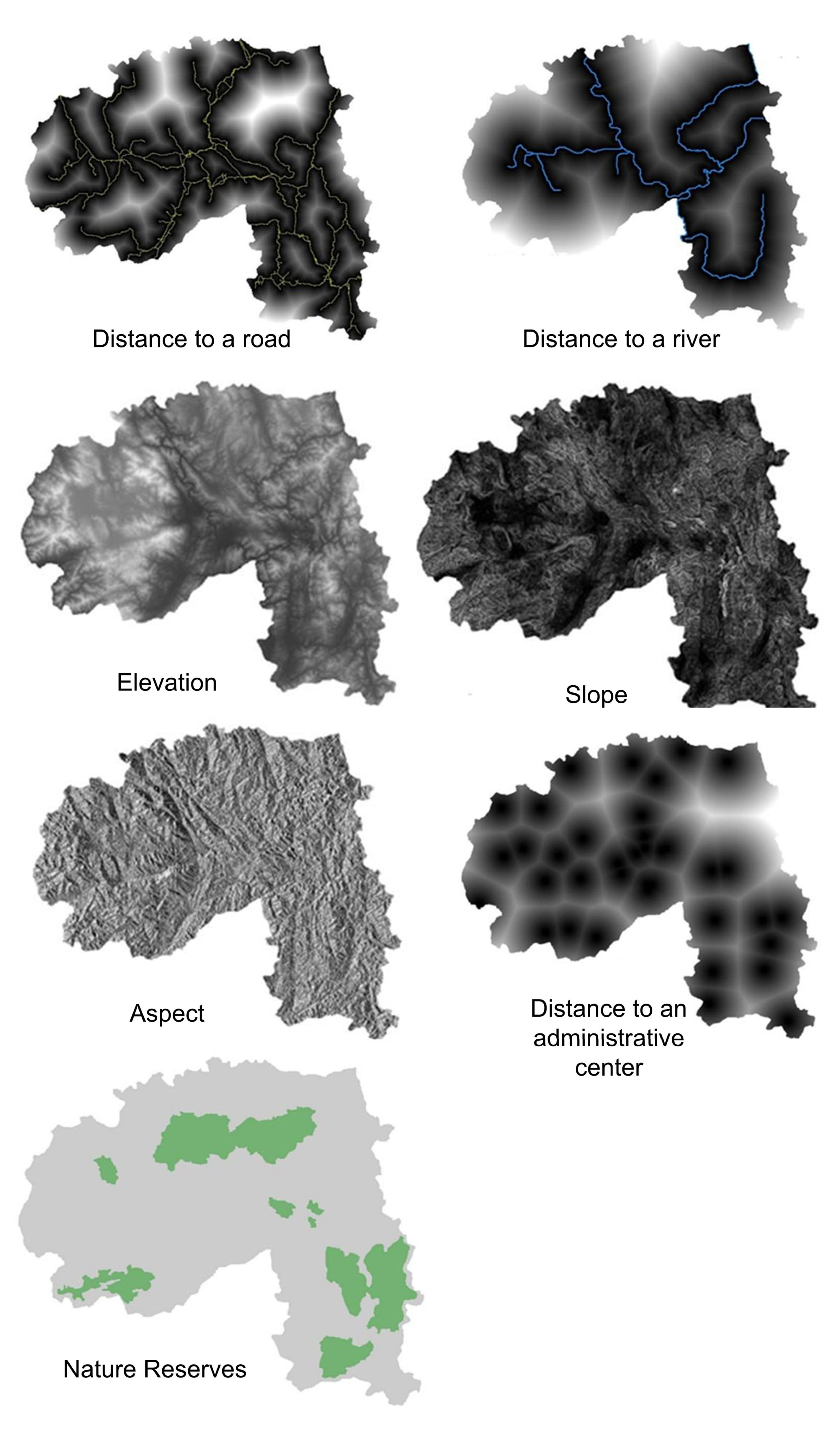
67]. Since RLs refer to the business-as-usual scenario, which means without any change in REDD+ drivers (situation, government, socio-economic forces, etc. that occur over time), this study only considered seven factors influencing land use change, namely distance to a road, distance to a river, elevation, slope, aspect, distance to an administrative center, and nature reserves (
Table 3 and
Figure 6).
Cramer’s V coefficients (
Table 4) were calculated to measure the correlation between the above-mentioned factors impacting land use change and land distribution. The larger the value, the stronger the correlation.
3.2.1. Distance to a Road
Besides playing a very important role in the economic and social development of a region, traffic conditions impact the land use status of a region. The overall correlation between the land type and distance from a road is 0.1334. Firstly, compared with the overall value, Cramer’s V coefficient for shrubland and tea gardens is 0.2735 and 0.2148, respectively, which is much higher than the overall value. Thus, the distance from a road is a relative important factor affecting shrubland and tea gardens. Secondly, Cramer’s V coefficient of the impact of the distance from a road on rubber plantations and construction land is 0.1550 and 0.1411, respectively, quite similar to the overall value. Thus, the affected land types dominated by road traffic in the Xishuangbanna region are shrubland, tea gardens, rubber plantations, and construction. It is evident that these land types are affected by anthropogenic activity. The reason of highest correlation between the shrubland and road is that it is very common in Xishuanbbanna to have roads built across shrubland rather other areas.
3.2.2. Distance to a River
The precipitation in Xishuangbanna region is abundant and evenly distributed. The dependence of most land use types on rivers is not obvious, except for shrubland and tea gardens. Among them, the influencing factor, namely the overall correlation value of the distance from a river to the land type is 0.0905, and the Cramer’s V coefficients for tea gardens (0.1277) are higher than this overall value. This result indicates that the distance from a river is the main factor affecting tea gardens.
3.2.3. Terrain-Related Factors
Topographic factors play a very important limiting role in various production activities. The study area is mainly mountainous, and, thus, the topographic factors of elevation, slope, and aspect cannot be ignored. Firstly, the overall value of the correlation is 0.2539, and woodland and rubber plantations alone show higher correlation coefficients than this overall value (the corresponding Cramer’s V coefficients are 0.3482 and 0.5297). During the period 1990–2010, the rubber plantation in Xishuangbanna continuously expanded from low-altitude flat valleys to mountainous areas in high altitudes due to high rubber price from the international market, population pressure, and economic development. This is the reason for the highest correlation between the elevation and rubber plantation. Cramer’s V coefficients of elevation for shrubland, grassland, cultivated land, tea gardens, construction land, and other land are 0.1192, 0.1289, 0.1355, 0.1230, 0.0451, and 0.2130, respectively, indicating that their correlation coefficients are lower than the overall value.
Secondly, the slope affects the water distribution, wind speed, and soil texture required for crop growth. The overall value of the correlation for the slope is 0.1608, while Cramer’s V coefficients for shrubland, rubber plantations, and tea gardens are 0.2131, 0.1984, and 0.1665, respectively, higher than the overall value. Thus, this factor can be regarded as the main factor impacting these land uses. However, in overall terms, Cramer’s V coefficient is less than the corresponding values for grassland, cultivated land, construction land, and other land (0.0406, 0.0210, 0.1076, and 0.0256, respectively).
Finally, the aspect primarily affects the length of time and temperature for the growth and final yield of crops. The overall value in this case is 0.0431, while Cramer’s V coefficients for shrubland, grassland, and rubber plantations are all greater than the overall value (0.0729, 0.0560, and 0.0570, respectively).
3.2.4. Distance to an Administrative Center
Governmental administrative organizations are typically located in townships. Given the increasingly strict forest protection policies being applied to Xishuangbanna region, areas closer to governmental administrative organizations can be conveniently supervised and regulated, resulting in a certain deterrent effect on forest destruction and illegal mining of local resources. The overall value of the distance from a township is 0.1252. The corresponding Cramer’s V coefficients for rubber plantations, and tea gardens (0.1542, and 0.1516, respectively) are higher than the overall value. However, the coefficients for grassland, cultivated land, construction land, and other land (namely, 0.0933, 0.0455, 0.1025, and 0.0361, respectively) are less than the overall value. Therefore, rubber plantations and tea gardens are clearly (and expectedly) impacted by distance to a township, whereas this is not so for the remaining land use types.
3.2.5. Limiting Factor (Nature Reserve)
Xishuangbanna Nature Reserve is a national nature reserve consisting of five small sub-reserves, namely the Mengyang, Menglun, Mengla, Shangyong, and Manzhang Reserves. These sub-reserves are not geographically connected to each other and cover a total area of 242,500 ha (242,500 × 104 m2). Notably, 12.68% of the total area of the Prefecture is allocated to nature conservation, namely the protection of the tropical forest ecosystem and its rare wildlife. Relatively little land change has been observed in the protected area, and man-made damage has also been effectively contained. In this study, the conversion rate of certain land use types, such as forestland, in the protected area was set to 0; in other words, anthropogenic activities in these areas are completely restricted.
3.3. Future Land Use Simulation Results and Inspection
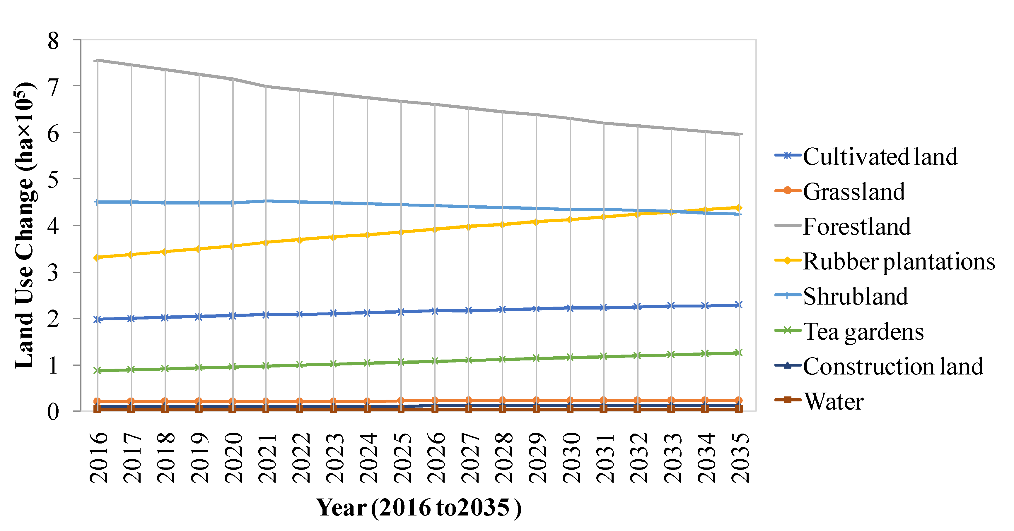
The expansion of rubber and other cash crops has caused massive forest loss and fragmentation in Xishuangbanna. The region experienced the most severe forest losses and degradation particularly for the period 1990 to 2010. Therefore, we chosen the period 1990 to 2010 for REDD+ in Xishuangbanna as the baseline, which is crucial to measure the emission reduction performance and consequently to negotiate meaningful deforestation emission reduction targets. As a result, the land use change data for 1990 and 2000 were used as inputs to the model of the Markov chain and MLP, and the 2010 land use change data were used as the verification values to simulate future land use. The validation of AUC value from the ROC curve method is 0.8, indicating that the results provided by the model are ideal. The land use prediction results for the Xishuangbanna region in the next 20 years of 2016–2035 are shown in
Figure 7.
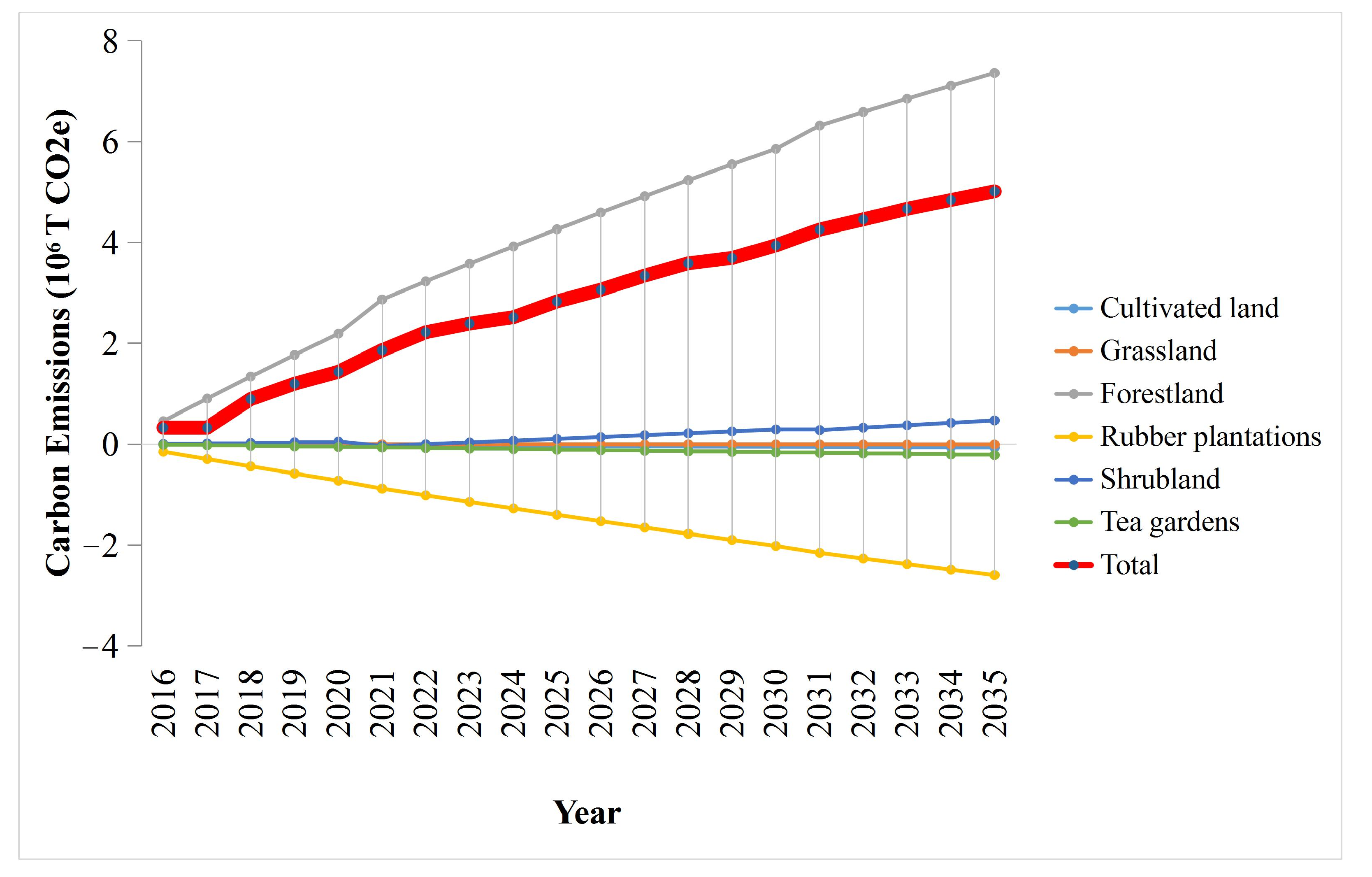
Area under forestland shows a downward trend and is the largest change over the 20 years, with the areal reduction amounting to 158,535 ha (158,535 × 104 m2). Conversely, the areas under rubber plantations, tea gardens, and cultivated land increase, with rubber plantations showing the highest increase (by 108,450 ha (108,450 × 104 m2)). The areas under tea gardens and cultivated land also increase, but only slightly (by 39,204 ha (39,204 × 104 m2) and 31,707 ha (31,707 × 104 m2), respectively). The areas under shrubland, grassland, construction land, and water bodies remained stable. Thus, in the next 20 years, the Xishuangbanna region will undergo further deforestation; simultaneously, given its improved economic development and the rising human demand for resources, the cultivation of cash crops such as rubber and tea will continue to increase, which will add pressure on the region’s forests.


