
Adaptive 3D Imaging for Moving Targets Based on a SIMO InISAR Imaging System in 0.2 THz Band


1
Aerospace Information Research Institute, Chinese Academy of Sciences, Beijing 100190, China
2
Key Laboratory of Electromagnetic Radiation and Sensing Technology, Chinese Academy of Sciences, Beijing 100190, China
3
School of Electronic, Electrical and Communication Engineering, University of Chinese Academy of Sciences, Beijing 100190, China
*
Author to whom correspondence should be addressed.
Remote Sens. 2021, 13(4), 782; https://doi.org/10.3390/rs13040782
Submission received: 26 January 2021
/
Revised: 16 February 2021
/
Accepted: 17 February 2021
/
Published: 20 February 2021
(This article belongs to the Special Issue Applications and New Trends in Metrology for Radar/LiDAR-Based Systems)
Abstract
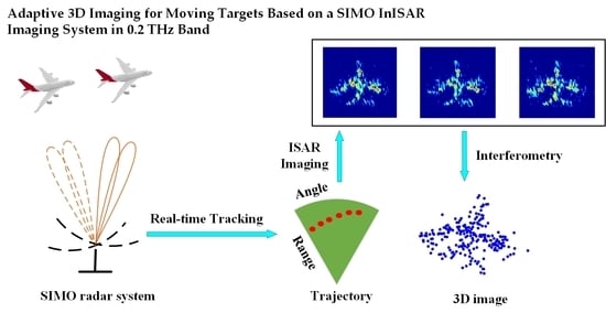
:Terahertz (THz) imaging technology has received increased attention in recent years and has been widely applied, whereas the three-dimensional (3D) imaging for moving targets remains to be solved. In this paper, an adaptive 3D imaging scheme is proposed based on a single input and multi-output (SIMO) interferometric inverse synthetic aperture radar (InISAR) imaging system to achieve 3D images of moving targets in THz band. With a specially designed SIMO antenna array, the angular information of the targets can be determined using the phase response difference in different receiving channels, which then enables accurate tracking by adaptively adjusting the antenna beam direction. On the basis of stable tracking, the high-resolution imaging can be achieved. A combined motion compensation method is proposed to produce well-focused and coherent inverse synthetic aperture radar (ISAR) images from different channels, based on which the interferometric imaging is performed, thus forming the 3D imaging results. Lastly, proof-of-principle experiments were performed with a 0.2 THz SIMO imaging system, verifying the effectiveness of the proposed scheme. Non-cooperative moving targets were accurately tracked and the 3D images obtained clearly identify the targets. Moreover, the dynamic imaging results of the moving targets were achieved. The promising results demonstrate the superiority of the proposed scheme over the existing THz imaging systems in realizing 3D imaging for moving targets. The proposed scheme shows great potential in detecting and monitoring moving targets with non-cooperative movement, including unmanned military vehicles and space debris.
1. Introduction
Terahertz (THz) waves lie in the gap between microwave and infrared, their frequency generally covers the band from 0.1 THz to 10 THz, corresponding to a wavelength from 3 mm to 30 um. Due to its special position in the electromagnetic spectrum from macro electronics to micro optics, THz waves possess many unique features [1]. Compared to microwaves, THz waves can achieve high imaging resolution thanks to their shorter wavelength and wider bandwidth. Compared to optic wave, THz waves are able to penetrate obscuring materials, such as clothing, plastics, wood, and dust, with relatively little loss. Besides, the photon energy of THz waves is much lower than the familiar X-ray, causing nearly no harm to human bodies. The above advantages show the great potential of THz imaging and sensing in plenty of applications [2], including public security detection [3,4,5,6,7,8,9,10,11,12,13,14,15,16], radar imaging [17,18,19,20,21,22,23,24,25,26,27], non-destructive inspection [28,29], and biomedical testing [30].
With the remarkable progress of THz devices in the past decades, a series of THz imaging systems have been developed for different applications. Depending on the working scenario, the current THz imaging systems can be classified into two types, one is the stationary scenario and the other is the cooperative moving scenario. In the stationary imaging scenario, the targets are required to keep static during imaging. A typical imaging scheme designed for this scenario is the beam-scanning system, where the beam is focused on a small spot and scanned over the imaging area by mechanical or optic-mechanical configuration. The image is obtained by processing the recorded echoes at each scanning grid [3,4,5,6,7].
The typical applications based on the beam-scanning scheme include the 0.35 THz standoff personnel screening system developed by the Pacific Northwest National Laboratory (PNNL) [3,4,5] and the 0.67 THz imaging system developed by the jet propulsion laboratory (JPL) for the similar purpose [6,7]. Although a high resolution can be achieved, the scanning scheme increases the imaging time consumption and system complexity. What’s worse, the imaging field of view (FOV) is limited. Another THz imaging scheme for the stationary scenario is the synthetic aperture radar (SAR) imaging [17,18,19,20,21], which realizes cross-range resolution by the movement of the radar system. Since the range resolution depends on the signal bandwidth, focused images can be obtained at any distance. With a combination of synthetic-aperture concept and quasi-optical scanning, a fan-beam imaging system in 0.2 THz band was also proposed [8]. However, in the SAR imaging scenario, the targets can only be observed within a limited window when the radar beam scans over the target area; thus the FOV is still limited.
As for the THz imaging system for cooperative moving scenario, mainly two schemes are investigated in the current research. The first is to promote the imaging frame rate, by integrating the multi-input and multi-output (MIMO) array to the beam-scanning system to simplify the scanning operation, which largely promotes the imaging efficiency [9,10,11,12,13,14,15,16]. A representative of this scheme is the Terascreen program launched by the Europe Union (EU) in 2013 [10]. This scheme combines the MIMO array with quasi-optical scanning, aiming to get the three-dimensional (3D) image of working passengers in a certain range. Besides, the R&S Corporation developed the Quick Personnel Security Scanner (QPS) system by designing a planner multi-static sparse array [11,12]. The scanner can achieve the high-quality images of humans with concealed objects in real-time, and has got commercial applications. Although the system can image the moving targets near real-time, the targets are only allowed to move in a pre-defined area. In the second scheme, the inverse synthetic-aperture radar (ISAR) technique is universally adopted [22,23,24,25]. In the reported research so far, high-resolution ISAR images of the moving targets on a turntable are obtained with THz radar systems, where the targets are resolved in the cross-range direction by exploiting the Doppler frequency induced by angular rotation of the targets. The 0.3 THz radar system Miranda300 developed by Fraunhofer Institute for High Frequency Physics and Radar Techniques (FHR) is a representative system of this scheme [23]. The system is able to get millimeter-scale ISAR images of the targets under turntable motion. However, ISAR imaging of targets with translational movement have not been reported by the current systems.
Recently, the interferometric technique is applied to the THz ISAR imaging system, for the purpose of acquiring the 3D images of moving targets. Researchers from the National University of Defense Technology (NUDT) developed an interferometric inverse synthetic aperture radar (InISAR) imaging system in the 0.22 THz band [26,27], and achieved 3D images of targets undergoing turntable rotation or equivalent translational movement. However, the effective FOV is still restricted by the antenna aperture, once the targets move out the FOV, they cannot be imaged continuously.
In this paper, a 3D adaptive imaging scheme for non-cooperative moving targets is proposed based on an InISAR system in the 0.2 THz band. With a specially designed single input and multi-output (SIMO) antenna array, the moving targets can be accurately located and tracked using the angle measuring technique based on phase-comparison monopulse technique, thus the imaging FOV can be adaptively adjusted as the targets move. With a combined motion compensation method proposed in this paper, focused and coherent ISAR images of the moving targets can be achieved by each receiving channel. Furthermore, since interferometric baselines are formed by different receiving channels, the target size information in the vertical and horizontal directions can be acquired by means of interferometry, which enables 3D imaging of the moving targets. Benefiting from the continuous observation, the system can get the 3D images of the targets in different windows, which provides more information about the dynamic target status.
In order to verify the proposed scheme, proof-of-principle experiments were conducted with a SIMO InISAR imaging system in 0.2 THz band. In the experiments, the targets undergo noncooperative motion at a range of 4.5 m from the imaging system. The targets were stably tracked and well-focused images were obtained. The excellent experimental results verified the effectiveness of the proposed imaging scheme and methods, which shows superior performance over the existing THz imaging system.
The remainder of the paper is organized as follows. The architecture of the SIMO InISAR imaging system is demonstrated in Section 2. Section 3 introduces the signal model and the target tracking method based on phase-comparison monopulse technique. Section 4 presents the proposed combined motion compensation method and the detailed InISAR imaging procedure. The experimental results are presented in Section 5. Finally, a conclusion is drawn in Section 6.
2. Architecture of the Terahertz SIMO InISAR Imaging System
2.1. The Architecture of the SIMO Antenna Array
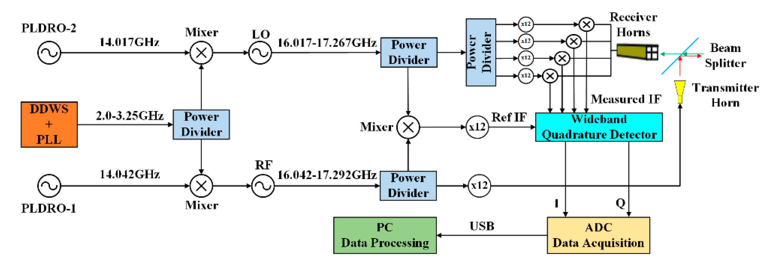
Figure 1 presents the block diagram of the SIMO InISAR system, which contains one transmitting channel and four receiving channels. To produce a wideband signal in the 0.2 THz band, the frequency multiply technique was adopted. The transmitting channel and receiving channels were connected to the corresponding transmitting chain and receiving chains, which are driven by the Ku-band radio frequency (RF) and local oscillator (LO) signals, respectively. To ensure an accurate synchronization between the RF and LO signals, based on the integration of a direct digital waveform synthesis (DDWS) module and phase locked loop (PLL) module, a fundamental frequency modulation continuous wave (FMCW) signal with a frequency range of 2.0-3.25 GHz was firstly produced and then split into two ways. One way is upconverted by a phase locked dielectric resonator oscillator (PLDRO) with a frequency of 14.042 GHz to get the RF FMCW signal, the other way is upconverted by another PLDRO with a frequency of 14.017 GHz to produce the LO FMCW signal. In the transmitting chain, the 0.2 THz signal was produced by upconverting the main branch of the RF signal with a ×12 multiplier. In the receiving chains, since heterodyne receivers are employed, the main branch of the LO signal was divided into four ways and then upconverted with four ×12 multipliers separately to form the THz LO signals for each channel. The measured intermediate frequency (IF) signals were acquired by processing the received echoes from the targets with de-chirping technology. In the IF module, the Ku band RF and LO FMCW signals were firstly mixed and then upconverted with a ×12 multiplier, resulting in the reference IF signal. Both the measured and reference IF signals were then sent to a multi-channel wideband quadrature detector to extract the amplitude and phase information of the received echoes, producing the I/Q signals. Finally, the signals were digitally sampled and transferred to the computer for data processing.
As for the antennas, a rectangular horn antenna was selected due to its simple structure and excellent radiation performance. The transmitting antenna is a single horn while the receiving antenna is a horn array which places four rectangular horns symmetrically in a plane, corresponding to four receiving channels. The aperture size of the receiving horn is 4 mm × 3 mm. The distances of the phase centers of two horns in the horizontal and vertical directions are both 5 mm, which equals the baseline length. Since no switchers are available in THz band, a high isolation is necessary between the transmitting and receiving channels. In this study, a quasi-optical isolator was designed by integrating a beam splitter and absorber, which not only isolate the transmitting and receiving channels effectively, but also lead to a compact antenna configuration. In the quasi-optical isolator, the beam splitter is deployed with a decline angle of 45°, the receiving horn array lies along the horizontal line crossing the center of the beam splitter, while the transmitting horn is rotated to the vertical direction with the center of the beam splitter as origin. This way, the wave paths from the beam splitter to the phase centers of the transmitting and receiving horns will be the same, eliminating the phase difference caused by the bistatic configuration of transmitting and receiving antennas. The prototype of the SIMO antenna array is shown in Figure 2.
2.2. FMCW Signal Model and De-chirp processing
Without considering the envelope information, suppose the radar works under the “stop-go” mode, the FMCW signal output from the transmitting antenna is expressed as:
where
where denotes the carrier frequency, means the chirp rate, means the chirp period. means the full time, where is the slow time and denotes the fast time which varies within a chirp period. Denoting as the bandwidth, then its value is determined as .
Suppose an ideal point scatterer, whose instantaneous range to the radar at slow time is . Ignoring the amplitude variation, the reflected signal arriving at the receiving antenna is expressed as:
where denotes the propagation speed of electromagnetic wave.
To receive the wide-band signal with lower sampling frequency, the system adopts a de-chirping receiver scheme which mixes the received signal with the LO signal to produce the IF signal. After demodulation and residual video phase (RVP) correction, the output signal from the IF module is expressed as:
It can be seen in (4) that the output IF signal of a point scatter is a single-frequency signal, and the following equation holds:
where means the frequency of the IF signal. It’s revealed that the frequency of the IF signal is proportional to the target range, so the sampling frequency can be determined by the expected detecting rang window. More detailed derivation can be found in [7].
Next, the range compression is accomplished by applying Inverse Fourier Transform (IFT) along the fast time, resulting in the high-resolution range profile (HRRP), which is expressed in the following form:
where means the wavelength of the carrier frequency.
Equation (6) indicates that the point spread function (PSF) of a single scatterer in the HRRP is a SINC function, the range information can be obtained from the HRRP according to the range cell in which the peak appears. As long as the wave path difference of scatterers from a target is larger than a range resolution cell, they will be projected into different range cells in the HRRP.
3. Adaptive Tracking of the Moving Targets Using Multiple Beams
3.1. SIMO Signal Model
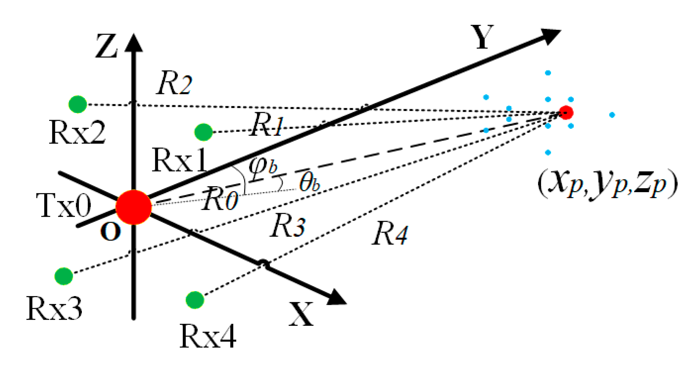
The geometry of the tracking and imaging scenario is illustrated in Figure 3. Taking the equivalent phase center of the transmitting antenna as the origin of the radar coordinate system, which is shown as the red dot denoted with “Tx0” in the figure. Shown as the green, the phase centers of the four receiving antennas locate symmetrically in the four quadrants of the XOZ plane, with their coordinates denoted as , , and , where Lx and denote the baseline lengths in the horizontal and vertical directions, respectively.
Without losing generality, suppose a rigid target which moves in the radar system with a vector velocity , the coordinates of a certain scatterer in the target are denoted as . Then the instantaneous range of the scatterer to the transmitting antenna is expressed as:
where Rp means the range of the scatterer in the initial position, means the radial velocity synthesized by the velocity vector along the three axes. The instantaneous range to the receiving antenna follows the formula:
where denotes the receiving channel number and is the coordinates of corresponding receiving antenna phase center.
Then, the received signal after de-chirping processing is expressed as:
And the corresponding HRRP is:
It is clear that the phase response of a certain scatter in the HRRP is determined by the close wave path from the transmitting antenna to the scatter center and then back to the receiving antenna. It’s also implied that the same scatter will respond differently in different receiving channels due to displacement of their antenna phase centers. However, since the baseline length is very short compared with the target range, a certain scatterer will appear in the same range cell on the HRRPs of different channels.
Besides, a sum channel signal can be synthesized by accumulating the echoes from the four receiving channels. In this study, the SIMO system can track the moving target continuously, which implies that the target is always located near the antenna axis during observation; thus the instantaneous target range to the transmitting antenna and receiving antennas are approximately identical under the very short baseline configuration. Moreover, in consideration of the symmetrical configuration of the four receiving horns, the phase difference induced by phase center displacement for each channel can be mitigated when accumulating the signals in the complex domain. As a result, the synthesized sum channel signal is expressed as:
And the HRRP of the synthesized sum channel has the following form:
The above expressions indicate that the phase component in the HRRP of the synthesized sum signal is determined by the round wave path from the transmitter antenna to the scatter center, which is equivalent to placing a virtual receiving antenna in the origin. Since the synthesis of the sum channel signal is a coherent accumulation, the SNR will be higher than the single channel, hence the target detection can be performed based on the HRRP of the virtual sum channel.
3.2. Target Locating with Phase Difference of Multiple Beams
Taking the advantage of multiple receiving channels of the system, the angular information of the targets can be acquired using the response difference in different channels according to the monopulse technique [31], making it possible to track the moving targets. Since the phase centers of the receiving antennas are located in the same plane along baselines lying in the azimuth and elevation directions, they constitute a typical antenna structure for phase-comparison monopulse technique, which accomplishes angle measurement by analyzing the phase response difference in different channels. Figure 4 gives an illustration of the angular measurement using the phase difference of two receiving channels. The red dot denoted with “Tx0” indicates the transmitting antenna, while the green dots denoted with “Rx1” and “Rx2” stand for the two receiving antennas. Under the plane-wave assumption, the wave paths in the two channels are different due to the displacement of their antennas, which will cause phase difference in the received echoes. The phase difference is mainly determined by the baseline length and target deviation angle , whose relationship obeys the formula:
In practice, the value of is usually obtained from the HRRPs of the receiving channels. The angular information can be immediately obtained with the following equation:
Generally, the angle measurement requires two receiving antennas which can form a baseline in a certain direction. A possible combination may be that Rx1 & Rx2 are used for azimuth angle measuring, and Rx1 & Rx4 are used for elevation angle measuring. Otherwise, the angle measurement in the azimuth direction can be accomplished using Rx3 & Rx4 couples, while the Rx3 & Rx2 couples can be used in elevation direction, with the same manner as shown in the above.
In this paper, in order to track the moving targets with high accuracy, a geometric center based tracking method is adopted. Since the large bandwidth of the FMCW signal enables a finer range resolution, scatterers from different parts of the targets can be resolved in the HRRP and the targets can be precisely located with the position information of multiple scatterers.
Without losing generality, three receiving channels Rx1, Rx2, and Rx4 were selected to illustrate the moving targets tracking processing with the SIMO system in this paper, and the whole flowchart is shown in Figure 5. Practically, the target tracking process includes the following steps. Firstly, the target detection is performed based on the HRRP of the virtual sum signal to detect the scatterers. Then, the angle measurement is performed to get the angular positions of each scatterer. Next, the geometric center of the target is synthesized using the range and angle information of the detected scatterers. After that, the measured results are input to a tracking filter to get a smooth and stable tracking trajectory. Finally, the antenna pointing direction is adaptively updated according to the output of tracking filter, ensuring a continuous beaming of the targets. Generally, the Kalman filter is preferred considering its robustness in most tracking scenarios [32]. If the targets undergo complex maneuvering movement, more comprehensive tracking algorithm like interactive multiple model (IMM) [33] can be selected. In this paper, since the targets mainly undergo translational movement, the Kalman filter is applied. In addition, to ensure a high tracking stability, the radar works in the step-tracking mode, which measures the target’s location using a consecutive number of echoes; more practical processing is explained in detail in [34].
4. Three-dimensional Imaging of Moving Targets with InISAR Technology
4.1. ISAR Imaging with Combined Motion Compensation
The adaptive tracking enables the continuous observation of the moving targets, which then provides a foundation for acquiring the high-resolution images using the ISAR imaging technique. Furthermore, the multiple receiving channels of the system make it possible to achieve the 3D imaging utilizing the interferometric technique. In this study, a combined motion compensation method was developed to fit in the special SIMO system configuration, with which the well-focused and coherent ISAR images are obtained for each channel.
Motion compensation is a critical procedure in ISAR imaging, which includes envelope alignment and phase correction [35]. The target range may vary during imaging interval and migration through range cell (MTRC) may occur, hence envelope alignment is necessary to remove the MTRC. After that, a phase correction is performed to eliminate the phase error caused by the noise or induced in range alignment operation.
In (7) and (8) it can be seen that the main part of the range term from the target to the receiving antenna is approximately equal to that to the transmitting antenna, so it’s practical to estimate the target movement component based on the virtual sum signal, whose phase history is dependent on the range from the target to the transmitting antenna. After the range alignment for the virtual sum channel is finished, time-varying phase errors may still exist along the slow-time, hence the phase correction is required to compensate this phase error, for the purpose of achieving focused ISAR images. In this paper, the phase gradient autofocus (PGA) algorithm [36] is applied to estimate the phase errors.
The estimated range migration and phase error based on the virtual sum signal are utilized to perform motion compensation on the four receiving channels, which is called combined motion compensation. This operation not only guarantees the coherence of the signals in different channels, but also improves the quality of compensation, considering the high SNR of the virtual sum signal.
The range profiles after combined motion compensation is expressed as:
where:
Once the motion compensation is done, the azimuth compression is then accomplished by applying Fourier Transform (FT) to the aligned range profiles along the slow time, which produces the ISAR images in the range-Doppler domain:
where denotes the integration time for imaging, denotes the Doppler frequency.
For the ISAR images of each channel, the Doppler frequency offsets caused by target motion along the baseline direction are denoted as and , which are determined by:
The phase component of the same scatterer in different images are expressed as:
Equation (19) indicates that the ISAR images in different receiving channels are mismatched in Doppler spectrum, which is induced by target motion and displacement of antenna phase centers. Equations (20) and (21) reveal that the amount of mismatch is determined by the length of baseline and target velocity.
4.2. Image Registration
As mentioned in the above section, a shift occurs among the ISAR images obtained by different receiving channels. Before performing the interferometric processing, image registration is required to align the images, which ensures that the same scatterer will appear in the same pixel in the ISAR images of different channels. In order to accomplish this goal, it’s essential to acquire the target moving velocities in the azimuth and vertical directions, with which the target motion can be compensated in the received echoes directly.
Fortunately, the target locations are measured and tracked during movement, and the values of and can be estimated by analyzing the recorded trajectory. Then the phase component to be compensated can be formed as follows:
For each receiving channel, a phase history is synthesized by substituting the coordinates of its antenna phase center to the above formula and then compensated in the corresponding raw signal.
After the image registration is performed, the ISAR images of the receiving channels will be shown in the range-Doppler domain with the following expressions:
It can be seen that the shift of ISAR images of different channels have been mitigated.
4.3. Interferometric Imaging
After image registration, the same scatterer will be projected onto the same pixel in the ISAR images of different channels, then the interferometric operation is performed to get the 3D imaging results. In this paper, channels Rx1, Rx2, and Rx4 are adopted to constitute the typical ‘L’ antenna array, which form interferometric baselines in the azimuth and vertical directions, respectively. According to (22), the phase responses of a certain scatter in the three images are expressed as:
Then the interferometric phases in each direction are extracted as:
This way, the target coordinates in the horizontal and vertical directions can be determined using the following equations:
It should be noted that since the targets are continuously tracked and the target size is far smaller than the target range, there is no need to consider the phase unwrapping under this situation. The target coordinate in the range direction is then calculated with the following formula:
By now, the coordinates of the target in the range, azimuth and vertical directions are all determined, and the 3D imaging results can be initially obtained. Figure 6 presents the whole flowchart of InISAR imaging procedure with the combined motion compensation method.
In order to illustrate the proposed InISAR imaging method based on combined motion compensation in a clear way, practical processing procedures with reference to Figure 6 are presented specifically in Table 2.
However, the section above discusses only the InISAR imaging procedure when the targets move in the front FOV of the radar, which is the same as the typical imaging scenario. But in this paper, since the antenna beams always keep illuminating the targets during tracking, the FOV is varying as the targets move, which is more complex than the typical situation. Thanks to the short wavelength of the THz wave, the Doppler frequency induced by target movement is so obvious that the integration interval can be greatly reduced to achieve a better resolution in azimuth direction. Therefore, the whole observation can be separated into several imaging windows, during which the instantaneous 3D images are obtained, hence making it possible to achieve a dynamic imaging to acquire information about the target status during movement.
In different imaging windows, the positions of the baseline will vary due to the adjustment of antenna pointing direction during tracking. Generally, a rotation angle of and around the azimuth axis and vertical axis will occur, as shown in Figure 3. A coordinate transform operation is necessary to get the imaging results in the global coordinate system.
The rotation matrices in the azimuth and vertical planes are defined as:
A coordinate rotation is performed on the initial 3D coordinates to get the target coordinates in the global coordinate system:
With the coordinate transform operation, the target images in different windows will be displayed in the same coordinate, which can be used to analyze the target status variation during tracking.
5. Experiments
5.1. Experiment Set-up
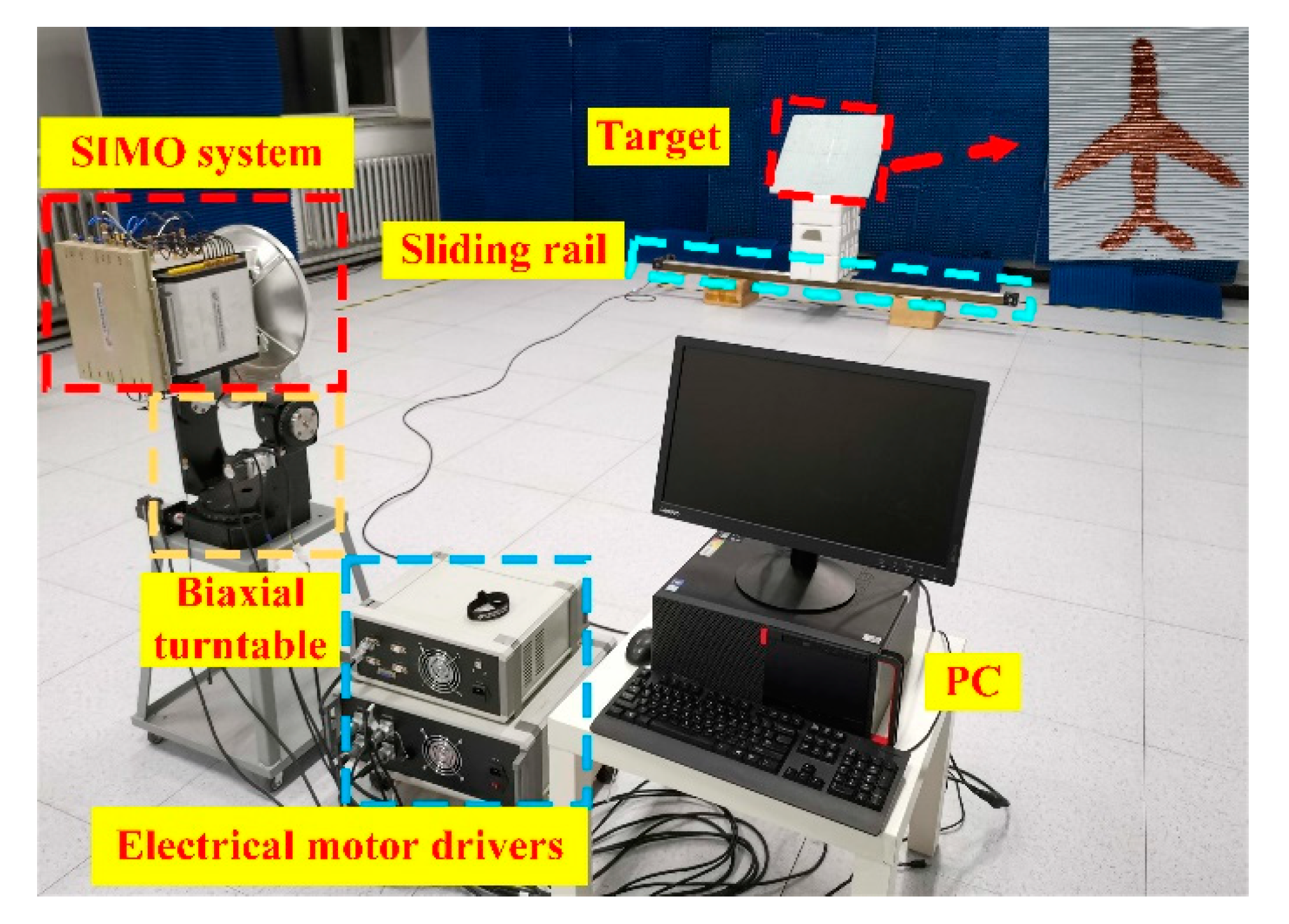
In order to verify the proposed scheme to achieve 3D images of the moving targets. Proof-of-principle experiments are carried out with the 0.2 THz SIMO imaging system in laboratory environment. The experiment scene is shown in Figure 7. The SIMO imaging system is fixed on a bi-axial turntable which works as the servo system to adjust the antenna beams in both azimuth and elevation planes. A sliding rail with a length of 2 m is used to move the targets, and the rail is driven by an electric motor which is remotely controlled by the computer. The sliding rail is symmetrically placed along the azimuth direction and its vertical distance to the radar is about 4.5 m. The targets are placed on a foam plate which is fixed on the sliding rail with the same height as the SIMO antenna array, and the foam plate is tilted with a pitch angle so that the targets are resolvable in the range direction. As shown in Figure 8, the target used in the experiments is a plane model painted with conductive paint coating, which is regarded as a complex target. The size of the model is about 25 cm in length and 20 cm in width. It has to be noted that, due to a lack of a 3D moving platform, only the horizontal motion is considered in this paper, but the tracking and imaging at the presence of 3D movement can be achieved with the same manner.
Before tracking, the antenna beam is firstly adjusted to capture the targets. As the targets move, the returned echoes are independently received by the four receiving antennas simultaneously and transferred to the computer for real-time processing. With the aim of obtaining stable tracking, the radar works at the step-tracking mode where a consecutive number of echoes are processed to locate the targets. In each step-tracking period, the servo system will adjust the antenna pointing direction adaptively to track the targets. Meanwhile, the received echoes are recorded in local disk for the purpose of imaging in the post-processing.
5.2. Target Tracking and Imaging
In the experiments, the targets were initially located in the left terminal of the sliding rail and move to the right terminal with a constant velocity of 0.052 m/s, with its coordinates varying from (-1.0 m, 4.5 m, 0) to (1.0 m, 4.5 m, 0). In consideration of both integration gain and tracking efficiency, the step-tracking period was set as 0.1 s, which means a number of 25 echoes are processed in each period. Consequently, the total tracking duration was about 38.5 s and 385 step-tracking periods were experienced, corresponding to 385 tracking records. Moreover, the actual positions of the targets during movement could be obtained from the parameters of sliding rail, which provided a reference for the evaluation of tracking accuracy. The parameters of the system and targets in the experiments are listed in Table 3.
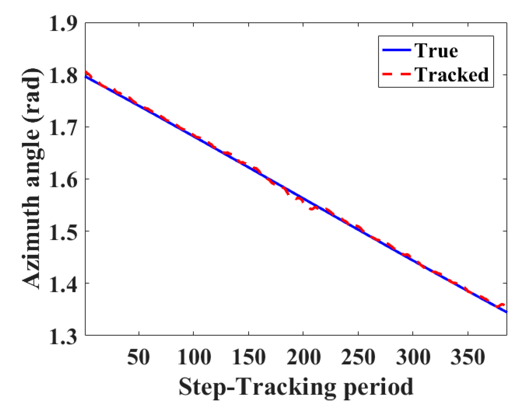
Figure 9 presents the tracking results of the plane model. Both the tracking result of azimuth angle and its comparison to the estimated true angle curve are shown in the figure. It’s seen from the curves that the tracked angular curve matches well with the real one, revealing a high stability of the tracking method. The estimated angular root mean square error (ARMSE) was 4.18 mrad, which satisfies the requirement of accurate tracking for imaging.
In post-processing, the recorded echoes from the moving targets during tracking were processed with the imaging method introduced in the above section. Figure 10 displays the ISAR imaging results of the plane model. Figure 10a presents the image produced by the virtual sum signal. The imaging time window is in the middle of the whole tracking duration. A number of 4096 echoes were processed, corresponding to an integration time of 16.384 s. The ISAR image is well-focused, which clearly shows the target shape and size information.
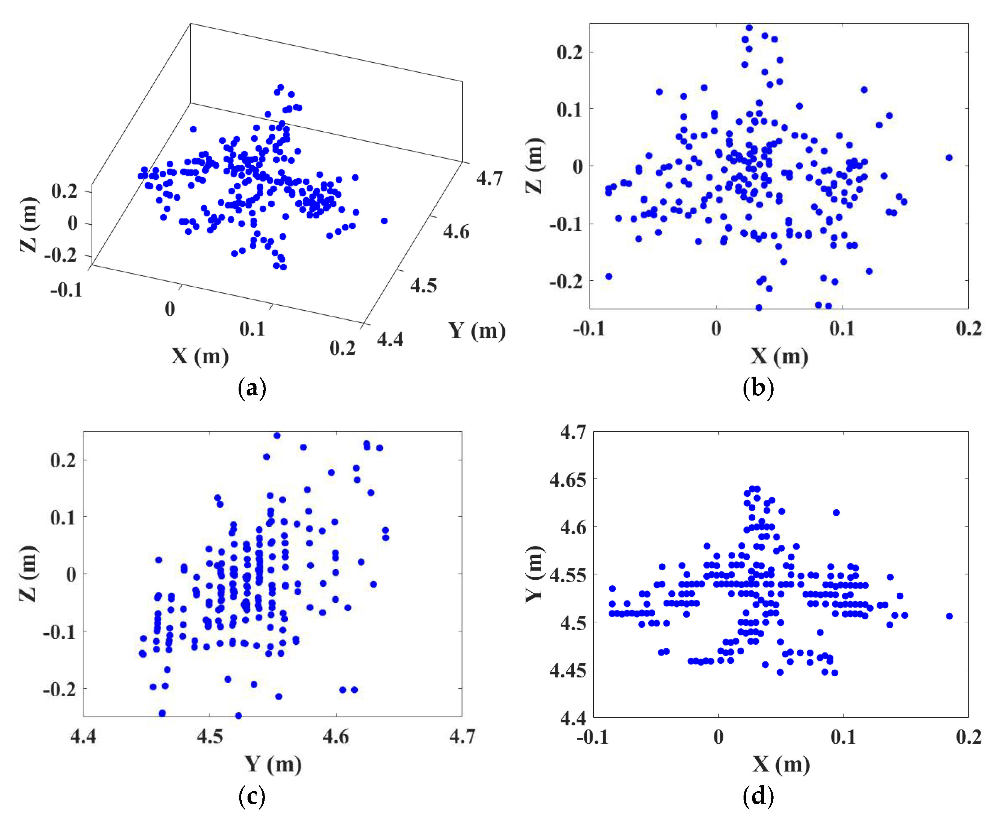
Next, the ISAR imaging for each receiving channel was performed using the same data set. Figure 10b–d show the ISAR images of the three channels (Rx1, Rx2, and Rx4) after the combined motion compensation processing. It can be seen that all of the three channels can image the moving targets with high quality. The interferometric imaging results are shown in Figure 11. Figure 11a–d display the 3D view, front view on the XOZ plane, side view on the YOZ plane, and bird’s eye view on the XOY plane, respectively. In order to guarantee the visual quality, only the pixels whose power level is higher than −10 dB are screened and applied interferometry. From the 3D images, the target shape and structure can be clearly identified, which are very similar to the real model.
Furthermore, the dynamic 3D imaging in different tracking periods was attempted. Another two imaging windows were selected from the whole observation, corresponding to the two periods during which the targets are moving in the left part and right part of the sliding rail. The window length was still set as 16.384 s and partially overlapped with the middle imaging window. Figure 12 displays the imaging results in the left window. The ISAR image acquired by the virtual sum signal and the 3D image are shown in Figure 12a,b, respectively. The corresponding ISAR and 3D imaging results in the right window are presented separately in Figure 13a,b. Due to the variation of observing view, the images in the side windows are slightly different with that in the middle, but the body of the model can be identified clearly.
The experimental results verify the feasibility and effectiveness of the proposed system. There is no doubt that the high-quality imaging results will support the target identification greatly and may find potential applications in many fields.
6. Conclusions
In this paper, a scheme to achieve 3D images of moving targets in THz band is proposed base on a SIMO InISAR imaging system. Based on the phase-comparison monopulse technique, the angular information of the targets is determined using the phase response difference in different receiving channels, which enables a real-time tracking of the moving targets with high accuracy. The continuous observation during tracking provides a foundation for high-resolution imaging. A combined motion compensation method was developed to accomplish the ISAR imaging, for the purpose of maintaining a good coherence among the images between different channels. The proposed scheme and methods were validated by the proof-of-principle experiments with a 0.2 THz SIMO system in the laboratory environment. The moving targets were tracked with a high angular accuracy and stability, based on which well-focused ISAR images and clear 3D images are obtained. Compared with the current THz imaging systems, this paper attempts acquiring the 3D images for moving targets for the first time. The promising results shown in the paper reveal the potential applications in tracking and imaging non-cooperative moving targets in many areas, like the supervision and identification of military targets or space debris.
Author Contributions
H.L. performed theoretical study, conducted the experiments, processed the data and wrote the manuscript. C.L. designed the imaging system and revised the manuscript together with S.W., S.Z. helped performing the experiments. G.F. provided the experiment equipment and funds for the research. All authors have read and agreed to the published version of the manuscript.
Funding
This work was supported by the National Key Research and Development Program of China (2018YFF01013004, 2017YFA0701004, 2018YFB2202500), and the National Natural Science Foundation of China (61671432, 61731020 and 61988102), and the Key project of equipment pre-research Fund (6140413010401), and the Science and Technology Key Project of Guangdong Province, China (2019B010157001), and the Key Program of Scientific and Technological Innovation from Chinese Academy of Sciences (KGFZD-135-18-029).
Institutional Review Board Statement
Not applicable.
Informed Consent Statement
Not applicable.
Data Availability Statement
No new data were created or analyzed in this study. Data sharing is not applicable to this article.
Acknowledgments
The authors would like to thank the editors and reviewers for their efforts to help the publication of this work.
Conflicts of Interest
The authors declare no conflict of interest.
References
- Horiuchi, N. Terahertz technology: Endless applications. Nat. Photon. 2010, 4, 140. [Google Scholar] [CrossRef]
- Popović, Z.; Grossman, E.N. THz metrology and instrumentation. IEEE Trans. THz Sci. Technol. 2011, 1, 133–144. [Google Scholar] [CrossRef]
- Sheen, D.M.; McMakin, D.L.; Hall, T.E. Three-dimensional millimeter-wave imaging for concealed weapon detection. IEEE Trans. Microw. Theory Tech. 2001, 49, 1581–1592. [Google Scholar] [CrossRef]
- Sheen, D.M.; McMakin, D.L.; Hall, T.E.; Severtsen, R.H. Active millimeter-wave standoff and portal imaging techniques for personnel screening. In Proceedings of the 2009 IEEE Conference on Technologies for Homeland Security, Boston, MA, USA, 11–12 May 2009; pp. 440–447. [Google Scholar]
- Sheen, D.M.; Hall, T.E.; Severtsen, R.H.; McMakin, D.L.; Hatchell, B.K.; Valdez, P.L.J. Standoff concealed weapon detection using a 350 GHz radar imaging system. Proc. SPIE 2010, 7670, 115–118. [Google Scholar]
- Cooper, K.B.; Dengler, R.J.; Llombart, N.; Bryllert, T.; Chattopadhyay, G.; Schlecht, E.; Gill, J.; Lee, C.; Skalare, A.; Mehdi, I.; et al. Penetrating 3-D imaging at 4- and 25-m range using a submillimeter-wave radar. IEEE Trans. Microw. Theory Tech. 2008, 56, 2771–2778. [Google Scholar] [CrossRef] [Green Version]
- Cooper, K.B.; Dengler, R.J.; Llombart, N.N.; Thomas, B.; Chattopadhyay, G.; Siegel, P.H. THz imaging radar for standoff personnel screening. IEEE Trans. Terahertz Sci. Technol. 2011, 1, 169–182. [Google Scholar] [CrossRef]
- Gu, S.; Li, C.; Gao, X.; Sun, Z.; Fang, G. Terahertz aperture synthesized imaging with fan-beam scanning for personnel screening. IEEE Trans. Microw. Theory Tech. 2012, 60, 3877–3885. [Google Scholar] [CrossRef]
- Saqueb, S.A.N.; Sertel, K. Multisensor Compressive Sensing for High Frame-Rate Imaging System in the THz Band. IEEE Trans. Terahertz Sci. Technol. 2019, 9, 520–523. [Google Scholar] [CrossRef]
- Alexander, N.E.; Alderman, B.; Allona, F.; Frijlink, P.; Gonzalo, R.; Hägelen, M.; Ibáñez, A.; Krozer, V.; Langford, M.L.; Limiti, E.; et al. TeraSCREEN: Multi-frequency multi-mode Terahertz screening for border checks. Proc. SPIE 2014, 9078, 907802. [Google Scholar]
- Ahmed, S.S.; Genghammer, A.; Schiessl, A.; Schmidt, L. Fully Electronic E-Band Personnel Imager of 2 m² Aperture Based on a Multistatic Architecture. IEEE Trans. Microw. Theory Tech. 2013, 61, 651–657. [Google Scholar] [CrossRef]
- Ahmed, S.S.; Schiessl, A.; Schmidt, L. A Novel Fully Electronic Active Real-Time Imager Based on a Planar Multistatic Sparse Array. IEEE Trans. Microw. Theory Tech. 2011, 59, 3567–3576. [Google Scholar] [CrossRef]
- Blazquez, B.; Cooper, K.B.; Llombart, N. Time-delay multiplexing with linear arrays of THz radar transceivers. IEEE Trans. Terahertz Sci. Technol. 2014, 4, 232–239. [Google Scholar] [CrossRef]
- Reck, T.; Kubiak, C.J.; Siles, J.V.; Lee, C.; Lin, R.; Chattopadhyay, G.; Mehdi, I.; Cooper, K. A silicon micromachined eight-pixel transceiver array for submillimeter-wave radar. IEEE Trans. Terahertz Sci. Technol. 2015, 5, 197–206. [Google Scholar] [CrossRef]
- Gao, H.; Li, C.; Zheng, S.; Wu, S.; Fang, G. Implementation of the phase shift migration in MIMO-sidelooking imaging at Terahertz band. IEEE Sens. J. 2019, 19, 9384–9393. [Google Scholar] [CrossRef]
- Gao, J.K.; Cui, Z.H.M.; Cheng, B.B.; Qin, Y.L.; Deng, X.J.; Deng, B.; Li, X.; Wang, H.Q. Fast three-dimensional image reconstruction of a standoff screening system in the Terahertz regime. IEEE Trans. Terahertz Sci. Technol. 2018, 8, 38–51. [Google Scholar] [CrossRef]
- Krozer, V.; Löffler, T.; Dall, J.; Kusk, A.; Eichhorn, F.; Olsson, R.K.; Buron, J.D.; Jepsen, P.U.; Zhurbenko, V.; Jensen, T. Terahertz imaging systems with aperture synthesis techniques. IEEE Trans. Microw. Theory Tech. 2010, 58, 2027–2039. [Google Scholar] [CrossRef]
- Stanko, S.; Palm, S.; Sommer, R.; Klöppel, F.; Caris, M.; Pohl, N. Millimeter resolution SAR imaging of infrastructure in the lower THz region using MIRANDA-300. In Proceedings of the 2016 46th European Microwave Conference, London, UK, 4–6 October 2016; pp. 1505–1508. [Google Scholar]
- Palm, S.; Sommer, R.; Homes, A.; Pohl, N.; Stilla, U. Mobile mapping by FMCW synthetic aperture radar operating at 300 GHz. In Proceedings of the International Archives of the Photogrammetry, Remote Sensing and Spatial Information Sciences, Prague, Czech Republic, 12–19 July 2016. [Google Scholar]
- Kim, S.; Fan, R.; Dominski, F. ViSAR: A 235 GHz radar for airborne applications. In Proceedings of the 2018 IEEE Radar Conference, Oklahoma City, OK, USA, 23–27 April 2018; pp. 1549–1554. [Google Scholar]
- Shi, S.; Li, C.; Hu, J.; Zhang, X.; Fang, G. Motion compensation for Terahertz synthetic aperture radar based on subaperture decomposition and minimum entropy theorem. IEEE Sens. J. 2010, 20, 14940–14949. [Google Scholar] [CrossRef]
- Danylov, A.A.; Goyette, T.M.; Waldman, J.; Coulombe, M.J.; Gatesman, A.J.; Giles, R.H.; Qian, X.; Chandrayan, N.; Vangala, S.; Termkoa, K.; et al. Terahertz inverse synthetic aperture radar (ISAR) imaging with a quantum cascade laser transmitter. Opt. Express 2010, 18, 16264–16272. [Google Scholar] [CrossRef] [PubMed]
- Caris, M.; Stanko, S.; Palm, S.; Sommer, R.; Wahlen, A.; Pohl, N. 300 GHz radar for high resolution SAR and ISAR applications. In Proceedings of the 2015 16th International Radar Symposium (IRS), Dresden, Germany, 24–26 June 2015; pp. 577–580. [Google Scholar]
- Cheng, B.; Jiang, G.; Wang, C.; Yang, C.; Cai, Y.; Chen, Q.; Huang, X.; Zeng, G.; Jiang, J.; Deng, X.; et al. Real-time imaging with a 140 GHz inverse synthetic aperture radar. IEEE Trans. Terahertz Sci. Technol. 2013, 5, 594–605. [Google Scholar] [CrossRef]
- Zhang, B.; Pi, Y.; Li, J. Terahertz imaging radar with inverse aperture synthesis techniques: System structure, signal processing, and experiment results. IEEE Sens. J. 2015, 15, 290–299. [Google Scholar] [CrossRef]
- Zhang, Y.; Yang, Q.; Deng, B.; Qin, Y.; Wang, H. Experimental research on interferometric inverse synthetic aperture radar imaging with multi-channel Terahertz radar system. Sensors 2019, 19, 2330. [Google Scholar] [CrossRef] [PubMed] [Green Version]
- Zhang, Y.; Yang, Q.; Deng, B.; Qin, Y.; Wang, H. Estimation of translational motion parameters in Terahertz interferometric inverse synthetic aperture radar (InISAR) imaging based on a strong scattering centers fusion technique. Remote Sens. 2019, 11, 1221. [Google Scholar] [CrossRef] [Green Version]
- Viegas, C.; Alderman, B.; Huggard, P.G.; Powell, J.; Parow-Souchon, K.; Firdaus, M.; Liu, H.; Duff, C.I.; Sloan, R. Active millimeter-wave radiometry for nondestructive testing/evaluation of composites glass fiber reinforced polymer. IEEE Trans. Microw. Theory Tech. 2017, 65, 641–650. [Google Scholar] [CrossRef]
- Meier, D.; Schwarze, T.; Link, T.; Zech, C.; Baumann, B.; Schlechtweg, M.; Kühn, J.; Rösch, M.; Reindl, L.M. Millimeter-Wave tomographic imaging of composite materials based on phase evaluation. IEEE Trans. Microw. Theory Tech. 2019, 67, 4055–4068. [Google Scholar] [CrossRef]
- Meo, S.D.; Espín-López, P.F.; Martellosio, A.; Pasian, M.; Matrone, G.; Bozzi, M.; Magenes, G.; Mazzanti, A.; Perregrini, L.; Svelto, F.; et al. On the feasibility of breast cancer imaging systems at millimeter-waves frequencies. IEEE Trans. Microw. Theory Tech. 2017, 65, 1795–1806. [Google Scholar] [CrossRef]
- Richards, M.A.; Scheer, J.A.; Holm, W.A. Principles of Modern Radar; SciTech Publishing: Edison, NJ, USA, 2010. [Google Scholar]
- Singer, R.A. Estimating optimal tracking filter performance for manned maneuvering targets. IEEE Trans. Aerosp. Electron. Syst. 1970, AES-6, 473–483. [Google Scholar] [CrossRef]
- Kirubarajan, T.; Bar-Shalom, Y. Kalman filter versus IMM estimator: When do we need the latter. IEEE Trans. Aerosp. Electron. Syst. 2003, 39, 1452–1457. [Google Scholar] [CrossRef]
- Li, H.; Li, C.; Gao, H.; Wu, S.; Fang, G. Study of moving targets tracking methods for a multi-beam tracking system in Terahertz band. IEEE Sens. J. 2020. [Google Scholar] [CrossRef]
- Zhu, D.; Wang, L.; Yu, Y.; Tao, Q.; Zhu, Z. Robust ISAR range alignment via minimizing the entropy of the average range profile. IEEE Geosci. Remote Sens. Lett. 2009, 6, 204–208. [Google Scholar]
- Wahl, D.E.; Eichel, P.H.; Ghiglia, D.C. Phase gradient autofocus—A robust tool for high resolution SAR phase correction. IEEE Trans. Aerosp. Electron. Syst. 1994, 30, 827–835. [Google Scholar] [CrossRef] [Green Version]
Figure 1.
Block diagram of the single input and multi-output (SIMO) system.

Figure 2.
Prototype of the SIMO antenna array.

Figure 3.
Geometry of the tracking and imaging scenario.

Figure 4.
Illustration of angle measurement with phase difference.

Figure 5.
Flowchart of target locating and tracking with multiple beams.

Figure 6.
The interferometric inverse synthetic aperture radar (InISAR) imaging processing flowchart based on combined motion compensation.
Figure 6.
The interferometric inverse synthetic aperture radar (InISAR) imaging processing flowchart based on combined motion compensation.

Figure 7.
The experiment set-up in laboratory environment.

Figure 8.
The painted plane model used in the experiments.

Figure 9.
Azimuth tracking results of the plane model.

Figure 10.
ISAR images of the plane model obtained by the (a) virtual sum signal, and receiving channels (b) Rx1, (c) Rx2, and (d) Rx4.
Figure 10.
ISAR images of the plane model obtained by the (a) virtual sum signal, and receiving channels (b) Rx1, (c) Rx2, and (d) Rx4.

Figure 11.
InISAR imaging results of the plane model. (a) The 3D view, (b) the front view, (c) the side view, and (d) the bird view.
Figure 11.
InISAR imaging results of the plane model. (a) The 3D view, (b) the front view, (c) the side view, and (d) the bird view.

Figure 12.
ISAR and InISAR imaging results of the moving target in the left window. (a) 2D ISAR image, (b) 3D InISAR image.
Figure 12.
ISAR and InISAR imaging results of the moving target in the left window. (a) 2D ISAR image, (b) 3D InISAR image.

Figure 13.
ISAR and InISAR imaging results of the moving target in the right window. (a) 2D ISAR image, (b) 3D InISAR image.
Figure 13.
ISAR and InISAR imaging results of the moving target in the right window. (a) 2D ISAR image, (b) 3D InISAR image.


Table 1.
Detailed procedures of the target locating and tracking.
| Input: Received raw echoes from Rx1–Rx4 in real-time. |
| Step 1: Synthesize the virtual sum signal by accumulating the echoes from the four receiving channels, and extract the echoes from Rx1, Rx2, and Rx4. |
| Step 2: Perform range compression to produce the HRRPs for the virtual sum channel, receiving channel Rx1, Rx2, and Rx4. |
| Step 3: Conduct target detection based on the virtual sum HRRP to find the range cells in which scatterers locate. The range information of each detected scatterer can be obtained at the same time. |
| Step 4: Extract the complex responses of each scatterer in the HRRPs of Rx1, Rx2, and Rx4 according to their range cell numbers. Then extract the phase response differences in the two receiver couples Rx1 & Rx2 and Rx1 & Rx4, respectively. |
| Step 5: For each scatterer, following equation (14), calculate its azimuth deviation angle with the phase response difference of Rx1 & Rx2, and calculate its elevation deviation angle with the phase response difference of Rx1 & Rx4. |
| Step 6: Determine the coordinates of each scatterer using corresponding range and angle information obtained in Step 3 and Step 5. Then synthesize the target geometric center to realize target locating. |
| Step 7: Perform Kalman filtering to get the tracking result, based on which the relative deviation of target from the antenna axis can be determined. |
| Step 8: Adjust the antenna pointing direction according to the relative deviation. |
| Output: Real-time tracking of the moving target. |
Table 2.
Practical procedures of the InISAR imaging.
| Input: Recorded raw echoes from Rx1-Rx4 during imaging windows. |
| Step 1: Synthesize the virtual sum signal by accumulating the echoes from the four receiving channels, and extract the echoes from Rx1, Rx2, and Rx4. |
| Step 2: Estimate the target moving velocities by analyzing the tracked trajectory. Then form the phase histories for corresponding channels according to equation (23) and compensate them in the raw echoes to accomplish image registration. |
| Step 3: Perform range compression to get the HRRPs of the virtual sum channel, receiving channel Rx1, Rx2, and Rx4. |
| Step 4: Estimate the range migration during imaging window baesd on the virtual sum HRRPs. Then perform combined envelope alignment by compensating the same range migration to the range profiles of Rx1, Rx2, and Rx4. |
| Step 5: Estimate the phase error history along slow-time baesd on the aligned virtual sum HRRPs. Then perform combined phase correction by compensating the same phase error history to the aligned range profiles of Rx1, Rx2, and Rx4. |
| Step 6: Conduct cross-range compression to get the ISAR images of the virtual sum channel, receiving channel Rx1, Rx2, and Rx4.. |
| Step 7: Perform interferometry for the ISAR images of Rx1 and Rx2 to obtain the scatterer coordinates in the horizontal direction according to equations (28) and (30). Meanwhile, perform interferometry for the ISAR images of Rx1 and Rx4 to obtain the scatterer coordinates in the vertical direction according to equations (29) and (31). |
| Step 8: Determine the scatterer coordinates in the range direction to acquire the 3D coordinates. |
| Output: 3D InISAR image. |
Table 3.
Parameters of the system and targets in the experiments.
| Parameter | Symbol | Value |
|---|---|---|
| Carrier frequency | 0.2 THz | |
| Bandwidth | 15 GHz | |
| Chirp period | 4 ms | |
| IF sampling frequency | 1.024 MHz | |
| Baseline length | , | 5 mm |
| Target size | --- | 25 cm × 20 cm |
| Target range | --- | 4.5 m |
| Target velocity | (0.052, 0, 0) m/s |
Publisher’s Note: MDPI stays neutral with regard to jurisdictional claims in published maps and institutional affiliations. |
© 2021 by the authors. Licensee MDPI, Basel, Switzerland. This article is an open access article distributed under the terms and conditions of the Creative Commons Attribution (CC BY) license (http://creativecommons.org/licenses/by/4.0/).
Share and Cite
MDPI and ACS Style
Li, H.; Li, C.; Wu, S.; Zheng, S.; Fang, G. Adaptive 3D Imaging for Moving Targets Based on a SIMO InISAR Imaging System in 0.2 THz Band. Remote Sens. 2021, 13, 782. https://doi.org/10.3390/rs13040782
AMA Style
Li H, Li C, Wu S, Zheng S, Fang G. Adaptive 3D Imaging for Moving Targets Based on a SIMO InISAR Imaging System in 0.2 THz Band. Remote Sensing. 2021; 13(4):782. https://doi.org/10.3390/rs13040782
Chicago/Turabian StyleLi, Hongwei, Chao Li, Shiyou Wu, Shen Zheng, and Guangyou Fang. 2021. "Adaptive 3D Imaging for Moving Targets Based on a SIMO InISAR Imaging System in 0.2 THz Band" Remote Sensing 13, no. 4: 782. https://doi.org/10.3390/rs13040782
Note that from the first issue of 2016, this journal uses article numbers instead of page numbers. See further details here.