
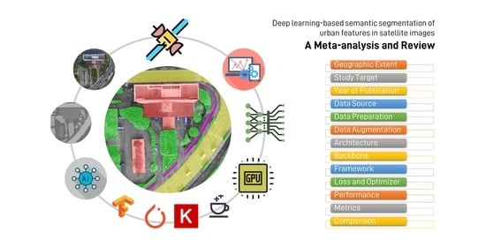
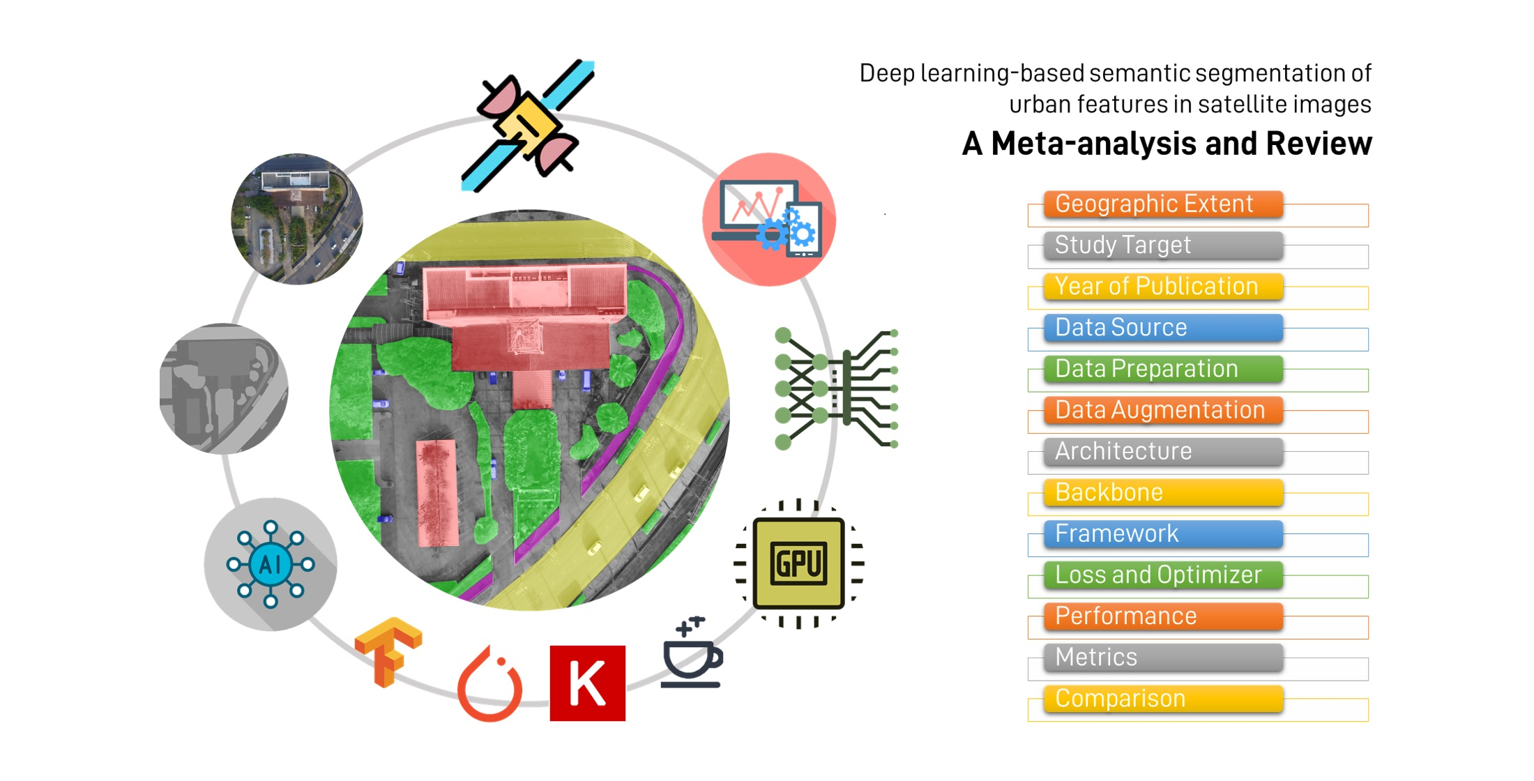
Deep Learning-Based Semantic Segmentation of Urban Features in Satellite Images: A Review and Meta-Analysis


1
Advanced Geospatial Technology Research Unit, Sirindhorn International Institute of Technology, 131 Moo 5, Tiwanon Road, Bangkadi, Mueang Pathumthani, Pathumthani 12000, Thailand
2
School of Information, Computer, and Communication Technology (ICT), Sirindhorn International Institute of Technology, 131 Moo 5, Tiwanon Road, Bangkadi, Mueang Pathumthani, Pathumthani 12000, Thailand
3
Department of Infrastructure Engineering, Faculty of Engineering and IT, The University of Melbourne, Melbourne, VIC 3010, Australia
*
Author to whom correspondence should be addressed.
Remote Sens. 2021, 13(4), 808; https://doi.org/10.3390/rs13040808
Submission received: 18 January 2021
/
Revised: 15 February 2021
/
Accepted: 18 February 2021
/
Published: 23 February 2021
(This article belongs to the Special Issue Deep Learning in Remote Sensing: Sample Datasets, Algorithms and Applications)
Abstract
:Availability of very high-resolution remote sensing images and advancement of deep learning methods have shifted the paradigm of image classification from pixel-based and object-based methods to deep learning-based semantic segmentation. This shift demands a structured analysis and revision of the current status on the research domain of deep learning-based semantic segmentation. The focus of this paper is on urban remote sensing images. We review and perform a meta-analysis to juxtapose recent papers in terms of research problems, data source, data preparation methods including pre-processing and augmentation techniques, training details on architectures, backbones, frameworks, optimizers, loss functions and other hyper-parameters and performance comparison. Our detailed review and meta-analysis show that deep learning not only outperforms traditional methods in terms of accuracy, but also addresses several challenges previously faced. Further, we provide future directions of research in this domain.
1. Introduction
Land-use/land-cover (LULC) maps are often generated from medium resolution satellite images like Sentinel [1] and Landsat [2]. These images are useful to classify land cover classes like built area, residential area, vegetation surface, impervious surface, water, etc. However, to prepare LULC maps for urban areas, objects like cars, individual buildings and trees, etc. needs to be classified. When extracting urban features or urban land cover information from aerial images, spatial resolution is considered being more important than spectral resolution. In other words, a finer-resolution image pixel is more useful than a greater number of spectral bands or narrower interval of wavelength [3]. This is the reason why commercial satellite images and unmanned aerial vehicles (UAV) are now more popular as they aim to increase the visibility of terrestrial objects, especially urban features, by reducing per-pixel size. With the increase in spatial resolution, more urban objects are now clearly visible in satellite images, and studies shifted its paradigm from spectral image classification, pixel-based image analysis (PBIA) and object-based image analysis (OBIA) to and most recently, pixel-level semantic segmentation. In this paper, we will analyse the advancement of deep learning-based semantic segmentation for urban LULC.
In early PBIA methods, the pixel size was not fine enough to identify an object in an image. As reported by Cowen et al. [4], a 4-m wide object needs a minimum of 2 by 2 m spatial resolution (i.e., minimum of four pixels is required). A 4 m wide object however does not locate perfectly over four pixels in a 2 m spatial resolution image. As the spatial resolution increased, the spectral response from different small objects in the urban area started to show complex patterns. This was because many objects are made of the same or similar material (e.g., cemented rooftops, cemented parking lots and cemented sidewalks; grasses and shrubs; etc.), and they emit a similar spectral response [5]. This is where the traditional classification methods and per-pixel classifiers (e.g., maximum likelihood) did not perform effectively because they used pixel-level spectral information alone as a fundamental basis to classify remote sensing images, and ignored spatial and contextual information [6]. Also, PBIA methods tended to produce “salt and pepper” noise after classification. To overcome these drawbacks, OBIA methods were studied.
Unlike PBIA, OBIA starts with the generation of segmented objects at multiple levels of scale as fundamental analysis units [7,8,9]. An object (aka. segment) in this approach is a group of contiguous homogeneous pixels with similar texture, spatial and/or spectral attributes. An image is initially divided into segments, various attributes of the segments are then computed and some rules are built to classify features. These rules are based on attributes such as geometry (length, area), size and textures etc., thus helping to differentiate features in an image. e.g., differentiating lakes and rivers based on length, trees from grass based on texture, separating building and road based on area, etc. For many years, OBIA was considered the better approach because it prioritized contextual information of an object [10]. Supervised and unsupervised learning classifiers methods were produced for the classification task, and PBIA was considered not as useful as OBIA to classify very high-resolution (VHR) images, until recently, after deep learning-based methods were started to be explored for pixel-based semantic segmentation of VHR images. In recent years, the use of UAVs to collect images and open-source/non-commercial software [11] to prepare orthomosaic have opened up a promising future towards the increased use of UAV-collected images. Despite the development of a large number of PBIA and OBIA-based methods proposed in the last two decades, these frameworks had several drawbacks [3] and complexities due to classification errors and imbalance in classes, which limited the widespread application. With recent end-to-end deep deep learning-based semantic segmentation, LULC has seen rapid progress in the classification of VHR images compared to traditional PBIA and OBIA methods.
Deep learning (DL) [12,13] architectures are modern machine learning methods that have increased the performance and precision of computation by increasing the number of “layers” or “depths”. DL allows fast and automatic feature extraction from an adequately large dataset, iteratively using complex models to reduce classification errors in regression [14]. In recent years, DL has become a core method in many researches in remote sensing, such as plant recognition [15], plant disease recognition [16,17], weed detection [18], crop type classification [19,20], crop counting [21], natural hazard modeling [22,23,24], land cover classification [25] and also uncertainty modeling [26]. DL architectures like convolutional neural networks (CNN) [27,28] and Fully Convolutional Network (FCN) [29] are commonly used methods for the segmentation of urban images. The most successful state-of-the-art DL architecture is FCN [30,31]. The main idea of this approach is to use a CNN as a powerful feature extractor while replacing the fully connected layers with convolution ones to output spatial maps instead of classification scores. Those maps are up-sampled to produce dense per-pixel output. This method allows training CNN in the end to end manner for segmentation with input images of arbitrary sizes. This approach achieved a notable enhancement in segmentation accuracy over common methods on standard dataset like Pattern Analysis, Statistical Modelling and Computational Learning (PASCAL) Visual Object Classes (VOC) [32]. However, the architecture of the FCN network is often changed to solve different challenges faced during semantic segmentation of urban satellite images.
A meta-analysis is performed in this paper to review the research papers that used DL-based methods to answer several research questions. A few review and meta-analysis papers have been recently published on a broader scope of the study, mostly focusing on a brief summary of recent trends on DL in remote sensing applications [33,34]. However, these studies do not provide detailed analysis in the domain of deep learning-based semantic segmentation of urban remote sensing images, which has been competitively and rigorously studied in the last 5 years as shown by our meta-analysis. Several studies improved image segmentation on urban features by designing efficient DL architectures, however there is a lack of a complete review on the technical details of the architectures experimented. In this paper, we present detailed and tabulated analysis and discuss how the recent papers have tried to address the challenges faced during the shift of paradigm to semantic segmentation such as: ignorance of spatial/contextual information by CNNs, boundary pixel classification problems, class imbalance problem, domain-shift problem, salt-and-pepper noise, structural stereotype, insufficient training and other limitations.
The rest of the paper is structured as follows: Section 2 presents literature on DL-based semantic segmentation of urban satellite images; Section 3 presents the complete meta-analysis on DL-based semantic segmentation; Section 4 provides discussions; and Section 5 concludes the paper with future directions. Furthermore, Appendix A, Appendix B and Appendix C are presented to display (i) the meta-analysis in structured summary, (ii) a separate performance comparison of papers that use the most abundant datasets and (iii) a list of the available dataset for DL-based semantic segmentation of urban images, respectively.
2. Deep Learning-Based Semantic Segmentation of Urban Remote Sensing Images
2.1. Semantic Segmentation in Remote Sensing
Semantic segmentation can be defined as the process of assigning a semantic label (aka. class) to each coherent region of an image. This coherent region can be a pixel, a sub-pixel, a super-pixel, or an image patch consisting of several pixels. Per-pixel segmentation classifies pixels by either assigning a single label to each pixel for high-resolution images, or assigning class membership on lower-resolution images because the resolution is not enough to contain an object [35]. Several parametric classifiers such as maximum likelihood classifiers and non-parametric classifiers such as artificial neural networks (ANN), support vector machine (SVM), decision tree classifiers, expert systems, etc. have been used in the past for per-pixel segmentation [10,36,37,38]. While the majority of ANN-based research was conducted for per-pixel classification in earlier days [39,40,41], sub-pixel classification of impervious surfaces were also highly studied later [42,43,44,45,46]. In sub-pixel classification, pixels are further classified into a fraction of the pixel size. Soon as the discovery of ANN, various networks were studied in early 2000s: Multi-layer Perceptron (MLP) [47,48,49,50], Adaptive Resonance Theory (ARTMAP), Self-Organizing Map (SOM) [51,52,53] and Hopfield Neural Networks. Superpixel is another coherent region for semantic segmentation of urban images [54,55,56]. These regions are first segmented on images using methods like Simple Linear Iterative Clustering (SLIC) [57] or superpixelization [58] to generate coherent regions at sub-object level.
In patch-based semantic segmentation, classifiers are trained on image patches as a single label and make predictions in a similar fashion. A sliding window is used to extract patches from the input images as bounding boxes around the object, which are further forwarded to predict label [21,23]. Multi-scale inference and re-current refinements performed significant gains on their study, and is also supported by other studies for scene labeling [59,60]. Patch-based segmentation performs well for object detection, but for the tasks like LULC, per-pixel methods often outperform the former method [55,61]. Some even consider patch-based methods wasteful because of redundant operations performed on adjacent patches [31].
As the resolution of satellite images increased, problems like loss of spatial information and imbalance of class distribution due to many small objects visible in an image resulted in many studies on pixel-based semantic-segmentation. Most studies in recent years have used DL-based semantic-segmentation to accurately label each pixel to a specific class like buildings, roads, etc. [62], which is further detailed in the next subsection.
2.2. Convolutional Neural Networks (CNN)
It was in 2006 that deep neural network (DNN) was once again brought to the spotlight, long after CNN was first proposed in [27]. DNN models like deep belief network (DBN) [63], autoencoders (AEs) [64], deep boltzmann machines (DBMs) [65], and stacked denoising autoencoders (SDAEs) [66] improved efficiency when training with large-scale samples. In 2012, AlexNet was proposed and achieved state-of-the-art on ImageNet classification benchmark [67]. After that, the networks started to take a deeper form in ZFNet [68], VGGNet (VGG16 and VGG19) [69] and GoogleNet [70].
The use of blocks consisting of separate architecture on its own and ensemble of the outputs using softmax layer is a general framework for CNN. Steps parametric rectified linear unit (PReLU) [71], dropout [72], batch normalization (BN) [73], and network optimizers like stochastic gradient descent (SGD) [74] and Adam Optimizer [75] are widely used to accelerate CNN training process. A standard structure of CNN consists of an input layer, convolutional layers, pooling layers, a fully connected layer and last the output soft-max layer. The output of each filter for a convolutional layer is calculated as
where and are the weights and bias term of th filter of th layer and denotes nonlinear activation function. A most commonly used activation function in CNN is rectified linear unit (ReLU) [71]. The weights and bias of each filter are passed to every location of the input feature map such that a model learns from the regrets of having applied the filter overlaid over any location of feature maps. A pooling layer like average-pooling and max-pooling are commonly used to provide shift-invariance by reducing the resolution of feature maps. The consecutive use of multiple convolutional and pooling layers produces smaller and abstract 2D feature maps, which are then connected by a sequence of fully connected layers that transform them into 1D features. The last softmax layer makes the final predictions.
CNNs are effective for object detection, scene-wise classification and feature extraction. However for pixel-based semantic segmentation, the use of pooling layers diminishes many features and the resulting feature maps and predictions cannot achieve the required PBIA. In the next section, we will talk about how FCN has improved the drawbacks of CNN.
2.3. Fully Convolutional Network (FCN)
When Long et al. [29] first proposed FCN in 2015, it achieved state-of-the-art semantic segmentation. What made it more efficient than CNN is that fully connected layers in a network for aerial image classification purposes can be considered as convolutions with kernels that cover their entire input region. Mou et al. [76] have considered this as equivalent to evaluating classification network on patches with overlapping regions. As the computation runs across images by overlapping the regions, FCN achieves better efficiency. And due to the presence of a pooling layer, feature maps obtained from FCN are then upsampled. CNN’s pooling layer aggregates information and extracts spatial-invariant features that are crucial for pixel-level semantic segmentation. A general framework of FCN therefore consists of two parts: encoders and decoders. Encoders are inspired from [66] and are similar to CNNs that extracts feature maps, and decoders transform these features into dense label maps, whose size is the same as the input image.
The first proposed FCNs were FCN-8s, FCN-16s and FCN-32s [29]. Instead of using simple bilinear interpolation, they used transpose convolutional layers to upsample the deep feature maps into labeling results. This improved the performance of classification resulting in finer predictions, but new challenges were born: (i) transpose convolutional layers were computationally expensive because of its hunger towards memory [77], (ii) they were difficult to train and (iii) the resulted classification was poor around the object’s boundary [76]. Several studies were thereafter performed to overcome these drawbacks. Chen et al. (2017) [78] introduced atrous convolutions in FCN, removing the max pooling layers, to expand the field of view with fewer parameters. To improve the classification errors around the boundary of label maps, they used conditional random fields (CRF) after FCNs. Ji et al. [79] introduced atrous convolutions on the first two layers of decoding steps to enlarge sight-of-view and integrate semantic information of large buildings, which are aggregated with multi-scale aggregation strategy. The last feature maps of each layer make predictions that are concatenated in the final prediction. Chen et al. (2019) [80] used FCN called DeepLabv3 [81] with Resnet backbone and atrous convolution layers, augmented Atrous Spatial Pyramid Pool (AASPP) with 4 dilated convolutional layers for multi-scale information and fusion layers to concatenate and merge the feature maps.
A mean-field approximate inference was used for CRF by Zheng et al. [82] with Gaussian pairwise potentials as recurrent neural fields (RNNs) to train an end-to-end CRF-as-RNN with unary energy of CRF. Lin et al. [83] later predicted both unary and pairwise energy using a deep structured model, which achieved significant performance on PASCAL VOC 2012 dataset. Most recently, Liu et al. (2019) [84] combined two pixel-level predictions—a pretrained FCN-8s fine-tuned and re-trained on 3-band image and probabilistic classifier called multinomial logistic regression (MLR) trained on LiDAR data—as unary potential modeled as CRF. They also used segments obtained from a gradient-based segmentation algorithm (GSEG) into a higher-order CRF called Potts’ model to resolve ambiguities by exploiting spatial-contextual information, and finally use graph-cut to efficiently infer the final semantic labeling for their proposed higher-order CRF (HCRF) framework. Apart from integrating CRF with FCNs, other network architectures were also designed for better classification, such as ResNet [85] based FCN [86,87].
Pyramid pooling module was proposed by Zhao et al. [88] in 2017, which was applied onto ResNet-based architecture to obtain clues on semantic categories distribution by parsing global information using large kernel pooling layers. Yang et al. [62] proposed end-to-end DL architecture to perform pixel-level understanding of high spatial resolution RS images, based on both local and global contextual information. They used the pyramid pooling module to collect multi-level global information. Low-dimension context representations were then upsampled by bilinear interpolation, thus obtaining representations with the same size as the original feature map. Finally, they concatenated multi-level global features and the last-layer convolutional feature map for the pixel-wise prediction. Yu et al. [89] proposed a pyramid scene parsing network (PSPNet) by incorporating cheaper network building blocks to extract multi-scale features for semantic segmentation. PSPNet comprised of two parts: (i) a CNN based on ResNet101-v2 to extract features by encoding input images into feature maps and (ii) a pyramid pooling module inspired from SPPNet [90] to extract features at multiple scales and upsample the feature maps to learn global contextual information by concatenating the multi-scale features. The final segmentation result is achieved by convolution operation on the concatenated feature maps. Later, Chen et al. (2018) [91] compared the use of ResNet-101 as the base structure for three baseline methods applied on roof segmentation: (i) feature pyramid network (FPN) (ii) FPN with multi-scale feature fusion (MSFF) and (iii) PSPNet; to observe the highest performance from PSPNet.
Different approaches of data fusion such as multi-modal, multi-scale and multi-kernel data fusion have also been practiced to improve the performance of FCN on RS images [56,80,91,92,93,94,95,96,97,98]. In a distinctive approach, some studies focused on the symmetry of the encoder-decoder structure, which is discussed in the next subsection.
2.4. Symmetrical FCNs with Skip Connections
Semantic segmentation requires both contextual information (object-level information) as well as low-level pixel data. Besides the pixel-level information, how to utilize contextual information is a key to formulate better semantic labeling. Contextual relationships therefore provide valuable information from neighborhood objects. In a symmetrical encoder-decoder FCN architecture, upper layers of encoders encode object-level information and lower layers capture rich spatial information. This information can become invariant to factors such as pose and appearance. And with skip connections, such networks can use both lower and higher-level information for finer predictions. This concept also helped the original U-Net architecture of Ronneberger et al. (2015) [99], in which each layer produces independent predictions. Multiple layers of convolutions, ReLU and max pooling combine the outputs of lower layers and higher layers to generate the final output. BN and ReLU are heavily applied to accelerate training and avoid vanishing gradient problems. These layers when trained using model optimizers such as SGD and back propagation (BP) of error, U-Net learns patterns. Finally, a softmax function generates the segmentation results. The model soon became widely used for medical image segmentation and also some studies can be found in urban images segmentation [100,101,102]. Yi et al. [103] proposed DeepResUnet for effective urban building segmentation at pixel-scale from VHR imagery. Their modification to the original U-Net included ResBlocks of two 3 × 3 and one 1 × 1 convolutional layers and ReLU activation functions. Compared to the original U-Net, DeepResUnet achieved better performance with fewer parameters, but with longer inference time. Yue et al. [104] proposed TreeUNet with DeepUNet [105] and Tree-CNN block to improve the differentiation of easily confused multi-classes. Tree-based CNN was later also used by Robinson et al. [106] to improve segmentation results with decision trees. Liu et al. (2020) [107] used two branches of modified U-Net to align feature distributions in the image domain and wavelet domain simultaneously, which were later merged to predict the final classification results. Diakogiannis et al. [108] proposed ResUnet-a, which uses U-Net’s encoder-decoder backbone, in combination with residual connections, atrous convolutions, pyramid scene parsing pooling and multi-tasking inference. SiameseDenseU-Net of Dong et al. (2020) [109] used two similar parallel DenseU-Nets [110] to alleviate boundary detection and class imbalance problems.
Another widely used symmetrical FCN is SegNet [111], which improved boundary delineation with minimum parameters by reusing pooling indices. Segnet is widely used in the domain of urban feature extraction, which can be seen later in Section 3.2.4. Many modified SegNet or used it as a backbone architecture [92,112,113,114,115] and some composed a new network using multiple FCNs like SegNet and U-Net [116,117]. Some used a network with multiple encoders of SegNet [113].
Several other symmetrical FCN networks have been proposed for urban image segmentation: DeconvNet [118], gated semantic segmentation network (GSN) [87], a network with boundaries obtained from edge detection [112] and SharpMask [119]. To boost the speed of segmentation compared to their original network called DeepMask [120], SharpMask produced features instead of independent predictions at all layers. Kemker et al. [121] adapted SharpMask and compared the results to RefineNet with ResNet-50 architecture, to observe similar performance results on urban feature classification. RefineNet [122] is similar to U-Net, but introduces several residual convolutional blocks inside the encoder and decoder. DeepLab networks—DeepLabv3 [81] and DeepLabv3+ [123] are other commonly used FCNs [104,124]. Chen et al. (2018) [125] introduced two semantic segmentation frameworks: Symmetrical normal shortcut fully convolutional networks (SNFCN) and Symmetrical dense-shortcut fully convolutional networks (SDFCN), both of which contain deep FCN with shortcut blocks. In order to properly fuse multi-level convolutional feature maps for semantic segmentation, Mou et al. [76] proposed a novel bidirectional network called “recurrent network in fully convolutional network” (RiFCN). Li et al. (2019) [126] used two separate sub-networks to make a Y-shaped network, whose final predicted feature maps are concatenated and merged using convolutional layers. The first sub-network is an FCN with skip-connections and the second sub-network is a network of 13 convolutional layers without downsampling layers to avoid loss of information. Sun et al. [115] proposed a novel residual architecture called ResegNet to solve the problem of “structural stereotype” and “insufficient learnings” that encoder-decoder architectures face.
2.5. Generative Adversarial Networks (GAN)
Most CNN based methods perform well when they are tested on the images that are similar to the train images, but fail when the domain shifts to a new domain. To address this problem and reduce the domain shift impact caused by imaging sensors, resolution and class representation, Benjdira et al. [127] modified the original GAN [128]. GAN consists of two models: generator and discriminator. A generator is trained to generate fake data to fool the discriminator, whereas discriminator is trained to differentiate between fake and real data. In Benjdira’s GAN, the generator follows a symmetrical encoder-decoder architecture and encoder consists of 4 convolutional layers for down-sampling and Leaky ReLU as an activation function. The output features extracted are passed to the decoder to rebuild the original feature vector. Decoder consists of four convolutional layers for up-sampling, standard ReLU as activation function and ‘dropout’ to reduce over-fitting. Instead of batch normalization, they used instance normalization. On the other hand, the discriminator consists of 5 convolutional layers that encode the generated image into a feature vector of a size of 256 × 256. Then, the sigmoid activation function in the last layer converts this feature vector into a binary output. Similar to the generator, Leaky ReLU activation function and instance normalization are used. The overall method can be summarized into the following steps: (i) Train segmentation model on source dataset. (ii) Train GAN to efficiently translate images from the source domain to the target domain. (iii) Convert the source dataset to the target domain using GAN, producing a new dataset with conserved structures of the source dataset but mimicking the global characteristics of the target dataset. (iv) Fine-tune the already trained segmentation model of step 1 with translated dataset associated with the source labels. Lin et al. [129] proposed an unsupervised model called multiple-layer feature-matching GAN (MARTA GANs) to learn a representation using only unlabeled data to increase the label dataset and Zhan et al. [130] designed a semi-supervised framework for hyper-spectral image data based on a 1-D GAN (HSGAN). Liu et al. (2020) [107] proposed a bispace alignment network called BSANet for domain adaptation (DA) and for automated labeling. BSANet uses two discriminators of modified U-Nets to minimize the discrepancy between the source and target domains. The use of GAN to solve the domain shift problems is limited and is expected to be studied more in the upcoming research works.
2.6. Transfer Learning
In order to increase the performance of a DL-model with fewer training samples and less computational power, some studies have used transfer learning [131]. Transfer learning allows the transfer of knowledge gained from solving one problem to be used for similar problems. The method has been quite popular in the studies that lack enough training images and labels [14,132,133]. Panboonyuen et al. [96] proposed to segment urban features in RS images using a global convolutional network (GCN) with channel attention blocks and domain specific transfer learning to transfer between learning obtained by training on VHR image to medium resolution images. Du et al. (2019) [134] performed semantic segmentation of crop (vegetation) area on RGB aerial images of Worldview-2. A DeepLabv3+ model pre-trained on ImageNet dataset was retrained on their dataset with image-GT (ground truth) label pairs. Compared to modern methods like U-Net, PSPNet, SegNet and DeepLabv2, and traditional machine learning methods like maximum likelihood (ML), SVM, and random forest (RF), their re-trained DeepLabv3+ model obtained the highest performance. Wurm et al. [135] segmented slum areas on RS images, in which they use transfer learning between models trained on different resolution images. Transfer Learning was done in two groups: (i) FCN based on VGG19 architecture that was pre-trained on ImageNet dataset transfers learnings and weights to three FCNs, trained on images collected from QuickBird (FCN-QB), Sentinel-2 (FCN-S2) and TerraSAR-X (FCN-TX). (ii) The learning of FCN-QB of the first group of the experiment was again transferred to FCN-S2 and FCN-TX. Some transfers produced better performance than others. Some studies use transfer learning to test their model in different ablations [79].
3. Meta-Analysis
3.1. Methods and Data for Review
Our methodology for bibliographical analysis in the domain under study follows three steps: (a) collection of related works (b) thorough study and (c) detailed meta-analysis. For the collection of related works, title search was performed in IEEE Xplore, ScienceDirect and Google Scholar using the search query [[“semantic segmentation”] OR [“pixel-level classification”] AND [“urban feature classification”] AND [“satellite imagery”]] on 21 December 2020. Also, more papers were downloaded from International Society for Photogrammetry and Remote Sensing (ISPRS)’s 2D Semantic Labeling Contest’s leaderboard for Vaihingen (Click the http://www2.isprs.org/commissions/comm2/wg4/vaihingen-2d-semantic-labeling-contest.html (accessed on 21 December 2020) to go to ISPRS’s leaderboard for Vaihingen dataset.) and Potsdam (Click the http://www2.isprs.org/commissions/comm2/wg4/potsdam-2d-semantic-labeling.html (accessed on 21 December 2020) to go to ISPRS’s leaderboard for Potsdam dataset). A total of 122 papers related to pixel-based classification of urban features were first downloaded.
Secondly, with thorough study, the papers that adapted object-based methods, traditional machine learning methods, performed vehicle segmentation and the studies that used terrestrial scene images, multi-view stereo (MVS) and Lidar for data collection were filtered out. Also, the technical reports that were not peer-reviewed papers were filtered out to select 71 papers that studied semantic segmentation of VHR satellite images for urban feature classification using DL-based methods. The 71 papers come from different countries. The countries of the first author’s affiliation are shown in Figure 1.
In the third step, the 71 papers filtered in the previous step were studied carefully to look for the trends and contributions of the 71 papers on the following five major research questions:
- What are the study targets?
- What are the data sources and datasets used?
- How is the training and testing data prepared for deep learning? This question looks for pre-processing, preparations and augmentation methods if used.
- What are the training details? This question looks for architecture, backbone, framework, optimizer, loss function and hyper-parameters that are mentioned by the papers?
- What is the overall performance of the method? This question looks for the performance metrics used, methods used for comparison, highest performance in each area of study and performance gains over previous methods.
3.2. Dissection and Overview of Research Questions
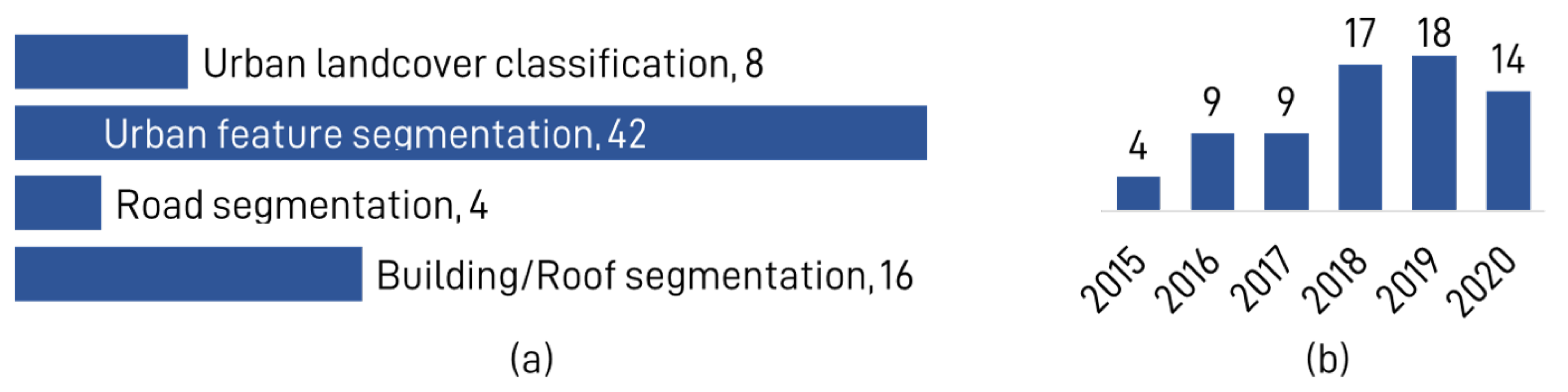
3.2.1. The Study Targets
The 71 papers can be divided into 4 study targets as building/roof segmentation, road segmentation, urban feature segmentation and urban land cover classification. Some papers intend multiple targets. The distribution is shown in Figure 2, which shows fewer studies on urban land cover [96,100,134,136,137,138,139]. With the availability of VHR images, smaller urban features have been segmented in the majority of papers. The papers that used dataset such as ISPRS Vaihingen 2D Semantic Labeling dataset, ISPRS Potsdam 2D Semantic Labeling dataset and IEEE GRSS (Geoscience and Remote Sensing Society) Data Fusion Contest (of Zeebrugge, Belgium) are dedicated to the improvement of semantic segmentation of urban features from traditionally interesting “urban area” class to Impervious surfaces, Building, Low vegetation, Tree, Car, Water, Boats and Clutter/background. Some have segmented urban features as small as sidewalk, motorcycles, traffic signs, pedestrians, picnic table, orange pad, buoy, rocks, sports courts, etc. [106,121,140,141]. Some classified buildings to their utilities [102,113], smaller features inside roads [142] and slum area [135]. Besides the segmentation of features, the studies use different approaches to improve semantic segmentation of urban features, which are shown in Table 1. The coherent regions used for segmentation are pixel, patch and super-pixel for 66, 4 and 2 papers respectively, including [143], which uses super-pixels to enhance pixel-based segmentation.
3.2.2. Data Sources
Among the 71 papers, most of them used a publicly available dataset consisting of a large number of images and labels, and some tested their model on multiple of these datasets. The most commonly used datasets are ISPRS Vaihingen 2D Semantic Labeling dataset [166] (38 papers) and ISPRS Potsdam 2D Semantic Labeling dataset [167] (27 papers) and IEEE GRSS Data Fusion Contest [168] (5 papers) collected their images using UAV. Other than UAV-based images, satellite images were obtained from RADARSAT-2 [136], Worldview-2 [102,134,156], Worldview-3 [149], Landsat-8 [96], SPOT [137,155], Gaofen [138,169], Quickbird, Sentinel-1 and 2 [147], Sentinel-2 and TerraSAR-X [135], PlanetScope (Dove constellations) [164]. A particular research collected data from a plane [140]. Some also used web-services such as Google Maps/Earth [140,161], World [101,140], Bing Maps [113] and Linz Data Service [103] often along with satellite images to improve segmentation results. Terrestrial data was also used for similar purposes [113]. For the comparison purpose or to assist the DL model, some used Lidar data. Lidar data were mostly included in the widely used public dataset mentioned before, and some used different ones. For VHR images, some prepared their own UAV-based dataset [121]. Some used Inria Aerial Image Labeling Dataset [76,114,117] for urban LULC. Other than urban LULC, some specific dataset dedicated for building/roof segmentation are Aerial Imagery for Roof Segmentation [91], SpaceNet building dataset [101], UK-based building dataset [160], WHU Building dataset [79]; for roads are AerialLanes18 dataset [142]; and for both roads and buildings is Massachusetts Building and Road Dataset (Mnih, 2013 dataset) [116,126,151,152,153,158,159]. Other dataset for building and roads are also used in [152,153]. More datasets that were found along with the details on resolution and web-source are provided in Appendix C. The spatial coverage of the 71 papers includes 46 local domain studies and 25 global domain studies. The local domain study means the dataset was collected within a single country and global domain study means the dataset was collected in more than one country.
3.2.3. Data Preparation
Here, we summarize the distribution of pre-processing, preparation and augmentation methods used. Pre-processing methods change the characteristics of images on pixel or spectral level. Some of these methods include image processing methods, image normalization by mean value subtraction on images [31,96,158,161], k-means clustering [134], relative radiometric calibration strategy [79], super-pixel segmentation [93], Lidar to digital surface model (DSM) [163], satellite image correction and pan-sharpening [102,164,169], normalized DSM (nDSM) and calculation of vegetation index such as normalized difference vegetation index (NDVI). Twenty-two papers performed such pre-processing methods. The most commonly performed methods calculation of DSM, nDSM, LiDAR data and NDVI [76,84,92,94,146,150]. Some used a stack of multiple channels of images [95,101,144,160]. Some used filters like unsharp mask filter, median filter, linear contrast filter [106] and Wiener filter [139]. Most papers that used datasets like ISPRS or IEEE did not perform pre-processing on images, because the images were already in a ready-to-use condition, and consisted of annotated labels too.
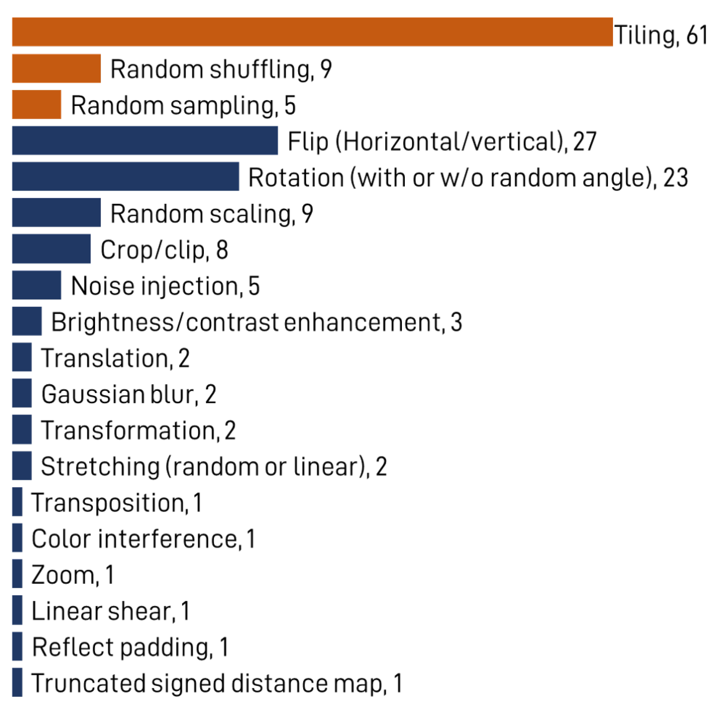
Data preparation includes methods used to prepare labels and images for train, test and validation dataset. The ratio of train-test/validation data is commonly 80-20 or 90-10. Image tiling is the most commonly used method and tile size was mostly 256 × 256 or 512 × 512 pixels. 18 papers overlapped the training tiles to their neighbors, among which most of them used 50% overlap. Yue et al. [104] used 2D Gaussian function to calculate the overlap. The distribution of these methods is shown in Figure 3. For the papers that used datasets like ISPRS and IEEE, the labels were already prepared. Others prepared labels manually [76,103,134,142] or used some traditional image segmenting methods to prepare labels [135,160]. The majority of papers (42 papers) have mentioned the use of image augmentation techniques to increase the number of training dataset or to increase the performance of overall learning procedure. The distribution of these methods is shown in Figure 3. Some also evaluated the increment in performance due to augmentation [95]. More details on this section can be found in Appendix A.
3.2.4. Training Details
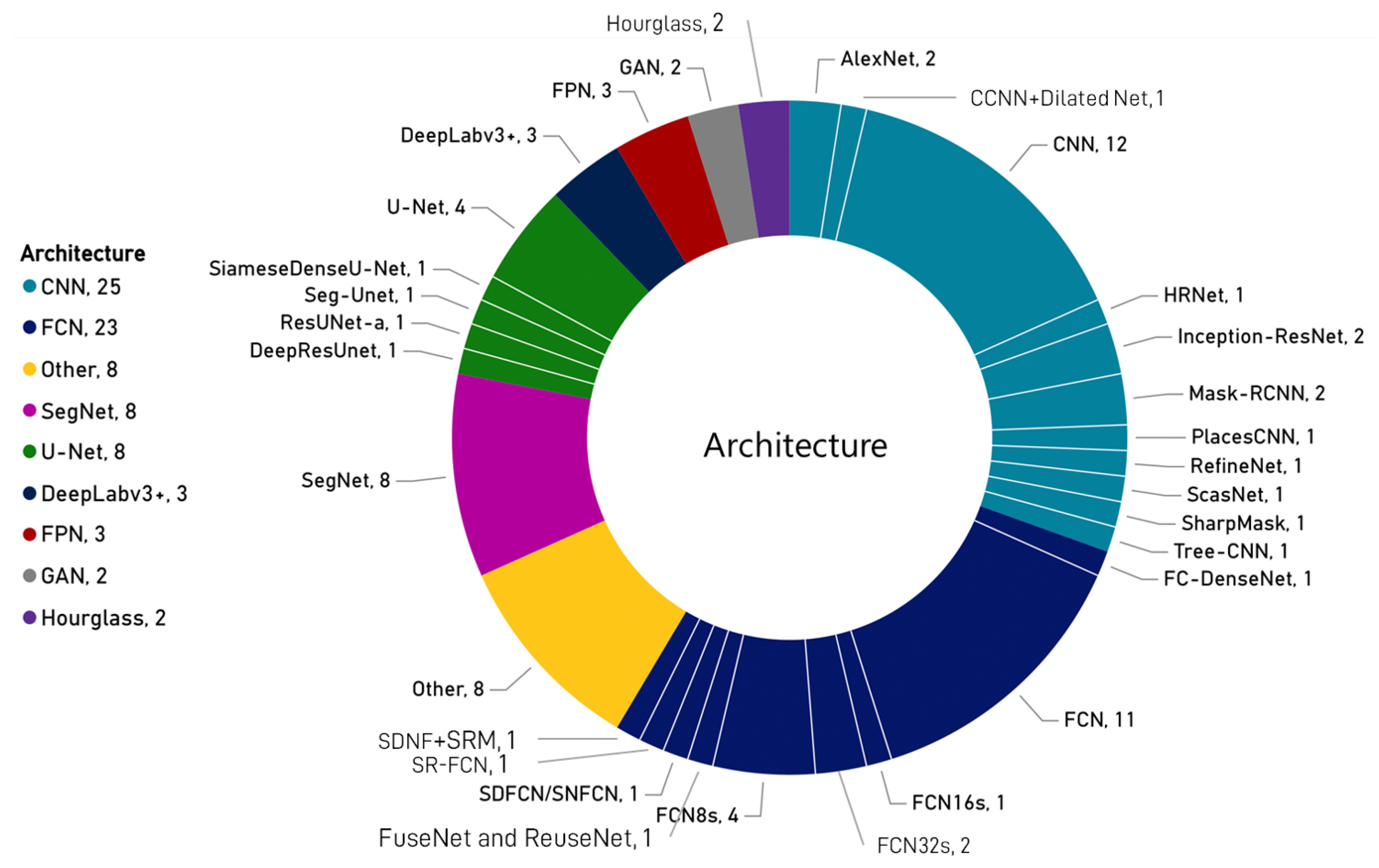
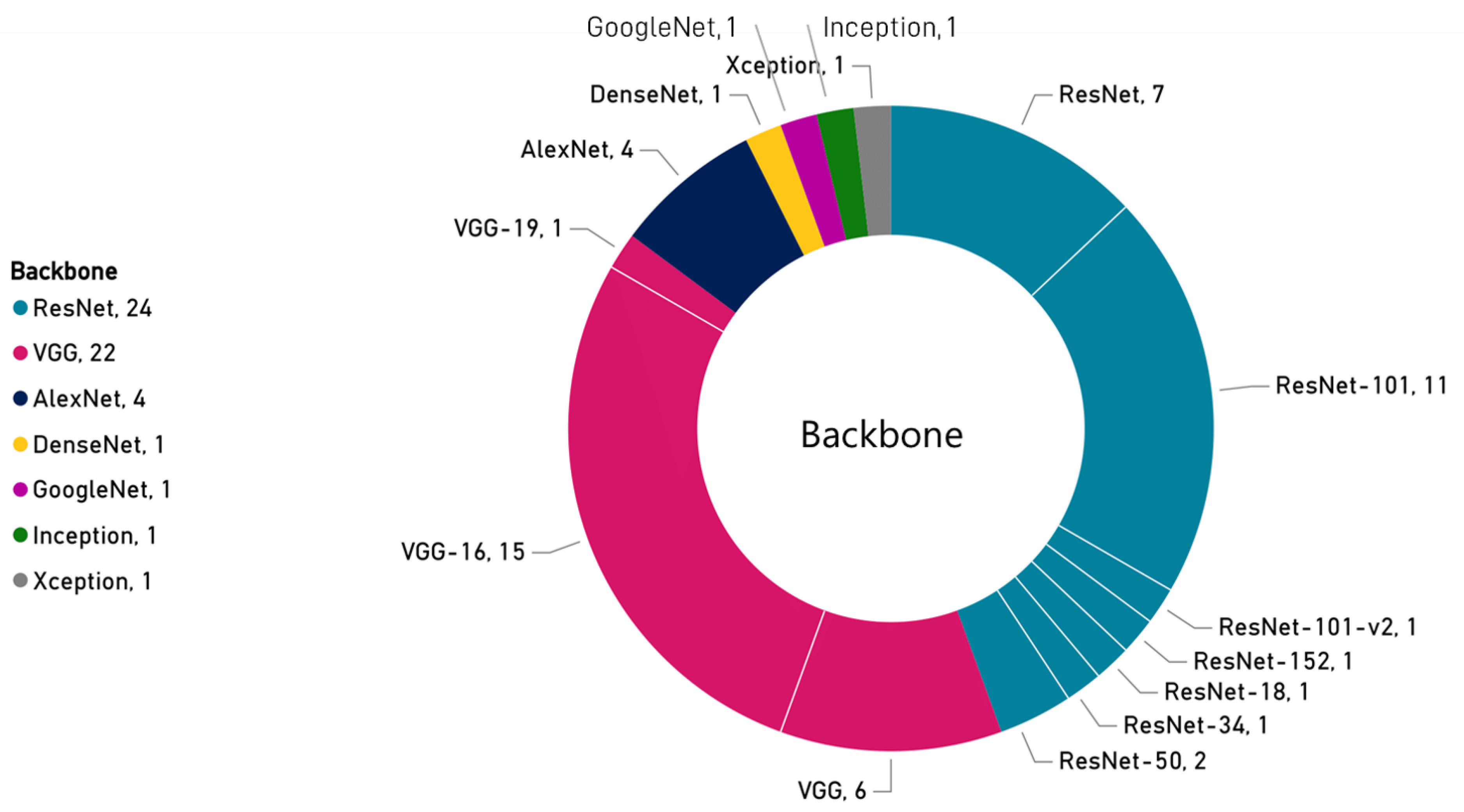
Training details include network architectures, frameworks, optimizers, loss function, hyper-parameters like learning rate, weight decay, momentum, epochs and iterations, use of dropout to handle over-fitting, and the hardware used by the papers. The architectures used are shown in Figure 4. The most commonly used architectures are CNN, SegNet, FCN, U-Net and FPN. More details can be found in Appendix A. Among the architectures used, SegNet, few FCNs, FPN, U-Net, DeepLabv3+, FSN, ResegNet, DeepUNet, ResUNet-a, DenseU-Net, FuseNet and ReuseNet are encoder-decoder structured architectures, mostly using skip connections (aka. skip branches). The convolutional backbones employed by the papers are shown in Figure 5. Among the papers that mentioned the name of the backbone used, the most commonly used ones are ResNet and Visual Geometry Group (VGG). The most commonly used ResNet backbone is ResNet-101, which helps in the reduction of vanishing gradient problem of deep learning. Other than convolutional backbones, some papers used DL architecture like SegNet and U-Net as a part of their model, making them the backbone of their new architecture.
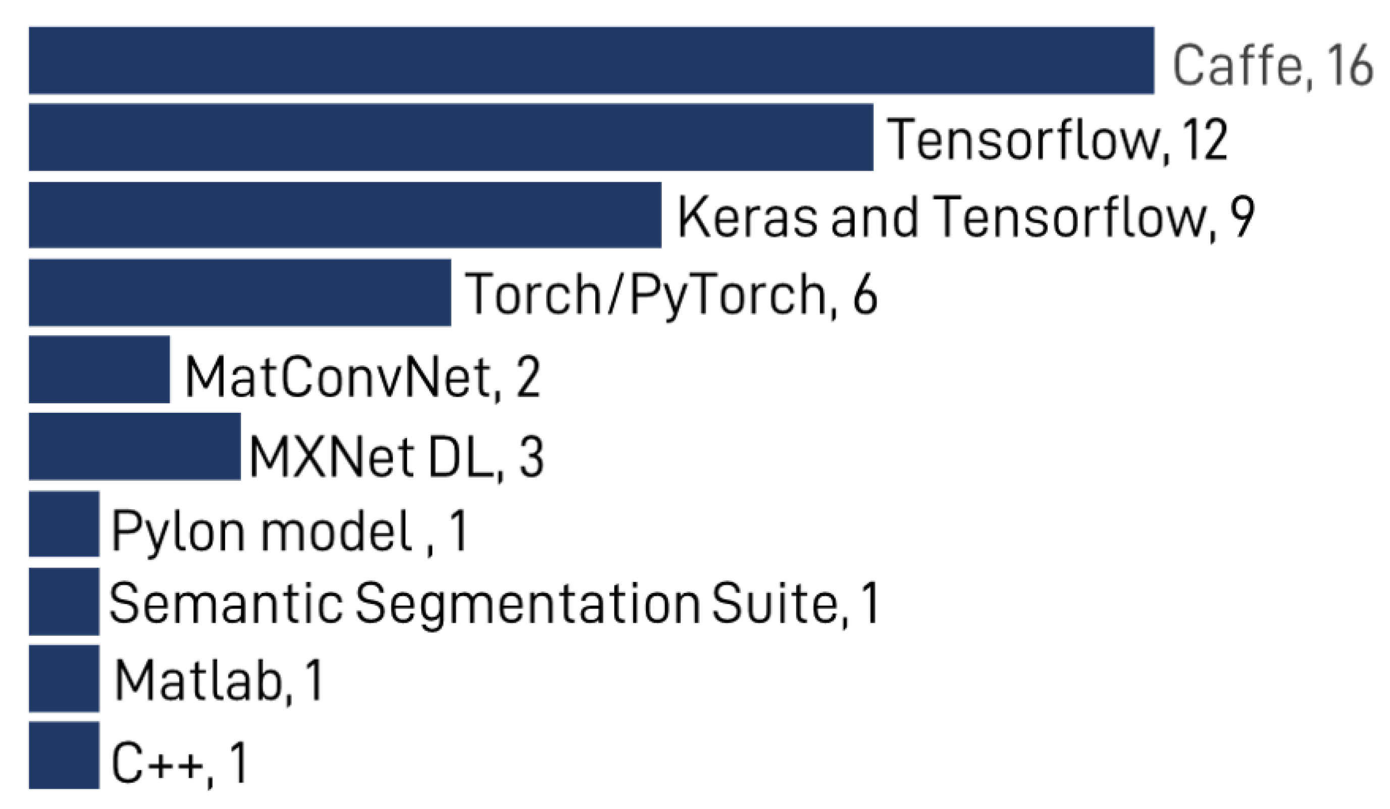
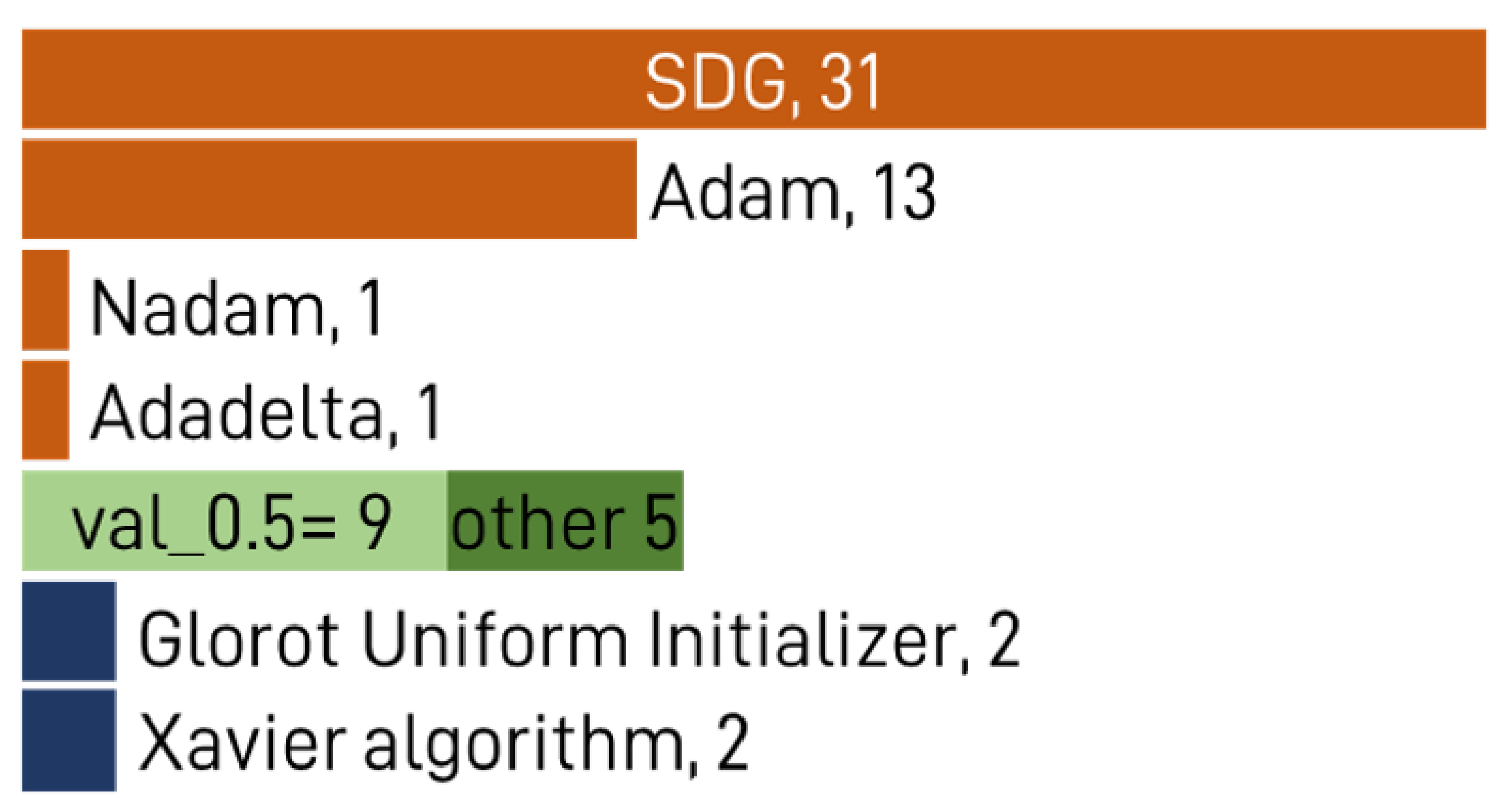
Talking about frameworks that are used to run or wrap the network architecture, the most commonly used were Caffe, Tensorflow, Keras and Torch. The distribution is shown in Figure 6 and details in Appendix A. Most commonly used network optimizers that optimize the network and keep off from model over-fitting are SGD including SGD with momentum or other hyper-parameters like learning rate. Other algorithms were Adam, Nadam (aka. Nesterov Adam) [76,121] and Adadelta [125]. Some used dropout functions to stop the over-fitting with common values of 0.5. To initialize the weights in the network, some used a special algorithm called Glorot Uniform Initializer [76,103] and Xavier algorithm [107,147]. The use of optimizers, dropout values and initializers are shown in Figure 7.
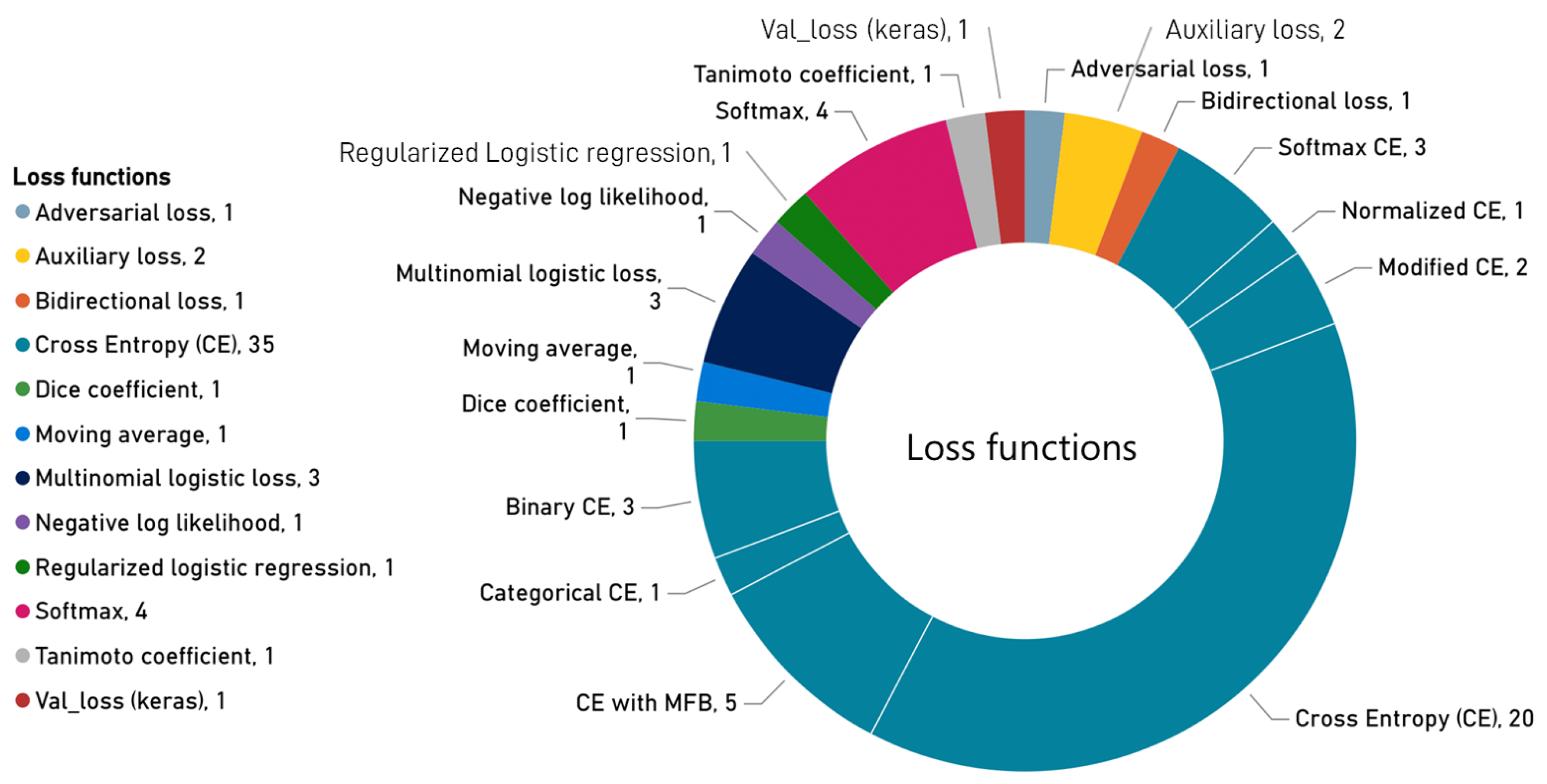
The loss functions that are used to evaluate how well specific algorithm models the given data include commonly used cross-entropy (CE) loss function (35 papers). The variety of CE loss used includes binary CE with semantic encoding loss [154], CE with median frequency balancing (MFB) [61,94,109,110,162], normalized CE [151], categorical CE function called logloss [125] and sparse softmax CE [135,148]. Some modified the CE loss [142,163] and compared the use of CE with MFB and CE with focal loss function weighted by MFB [110]. Other loss functions include auxiliary loss [62,89], adversarial loss [127], regularized logistic regression [144], multinomial logistic loss [146,147,161], validation loss from Keras [121], softmax [104,106,134,138], bidirectional loss [76], moving average [169], negative log likelihood loss (NLLLoss) [164] and Dice coefficient and Tanimoto coefficient [108]. The distribution of loss function is shown in Figure 8.
Hyper-parameters like learning rate, weight decay, momentum, epoch, batch size, number of iterations and steps are set up carefully as they depend upon the architecture, number of layers used and computer hardware specifications. The learning rate is either fixed or is decreasing with some decay rate of weight or momentum after a certain number of steps, iterations or epochs; ranging from 10 to 10. Most studies used graphics processing unit (GPU) units to train models faster (Figure 9). Most recent and powerful GPUs are used by the most recent papers, and all GPUs are from Nvidia.
3.2.5. Performance Comparison
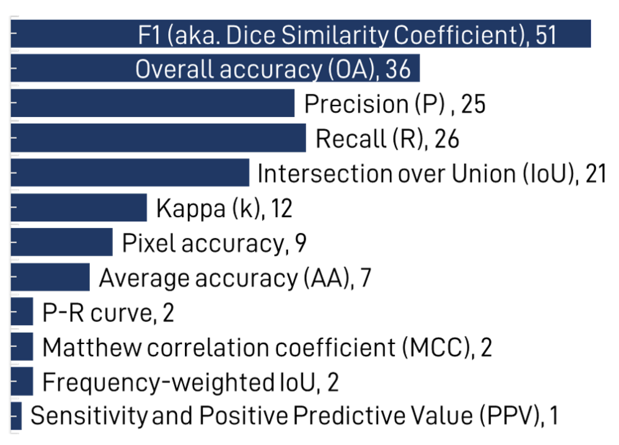
A wide range of metrics are used to evaluate the methods/models as seen in Figure 10 For simplicity, we refer to “DL performance” as the DL model’s performance score obtained from the metrics used in the papers. Most papers use multiple metrics to compare different combinations of same the model or to compare to other base models. The use of different experimental dataset and performance metrics makes performance comparison between different papers extremely difficult and often carries conviction. Therefore, we summarize the findings in the most meaningful ways by only comparing overall accuracy (OA) and F1 score among the papers that segmented multiple classes, and do not compare other metrics if these already exist OA. And some used k-fold cross validation in case the train and test dataset was small [135,137,146].
The papers that used common dataset have used similar metrics. Among the 32 papers that used ISPRS Vaihingen dataset and OA as the metric, OA ranged from 0.86 to 0.92 for the study target of “urban feature segmentation” with the highest value of 0.92 by superpixel-enhanced Deep Neural Forest (SDNF) [143]. For the ones that used F1 score, the highest of 0.92 was obtained by the ScasNet model (CASIA-2 in ISPRS leaderboard) [151]. Among the papers that used pixel accuracy, the highest of 0.87 was obtained. Similarly for the ISPRS Potsdam dataset, among the 23 papers that used the dataset for “urban feature segmentation”, OA ranged from 0.85 to 0.93 with the highest of 0.93 from 2 papers [143,147]. For the ones that used F1 score, the highest was 0.93 [98,108,151] and for the papers that used pixel accuracy, 0.87 was obtained. Potsdam data was also used for other study targets. The highest OA of 0.96 was obtained for “building/roof segmentation” [160].
For the dataset of IEEE GRSS, the highest OA of 0.90 was for “urban feature segmentation” [155] and for the Massachusetts Building dataset and Road Dataset, the highest was 0.97 [159] and 0.94 [153] respectively. For the other datasets used, the highest OA for each study targets are: 0.99 for “building/roof detection” [160], 0.96 for “urban feature segmentation” [76,156] and 0.99 for “urban land cover classification” [100]. For “Road segmentation”, 90% of roads were correctly segmented [159] and the highest F1 score of 0.94 was achieved [152].
It has to be noted that the objective of some papers [107,127] was not focused on producing the highest metric in segmentation, but was centered to improve the segmentation when the train and test datasets are from different domains. Benjdira’s method of GAN [127] improved OA from 35% to 52% when passing from Potsdam (source domain) to Vaihingen (target domain). Also, it improved the average segmentation accuracy of classes inverted due to sensor variation from 14% to 61%.
Out of all 71 papers, 62 compared their DL performance to some base models. Out of these, most (54 papers) compared to base models using modern DL architectures and 14 papers compared their results to traditional models. The traditional models include SVM [138], Extended Morphological Profiles (EMP) [156], conventional neural networks (NN) [152,158,159,170], Stochastic Expectation-Maximization (SEM) [136], Random Forest (RF) [55,102], Unary Potential Classifier [140], CRF, Simple Linear Iterative Clustering (SLIC) [137], maximum likelihood (ML) [134], k-nearest neighbor (kNN), Multi-layer Perceptron (MLP), multi-scale independent component analysis (MICA), stacked convolutional autoencoders (SCAE) [121], etc.
The trend shows that the more recent the research, the less are they being compared to traditional methods that do not use DL. Out of the 54 papers that compared their method to the modern DL-based methods, 38 papers used ISPRS’s Vaihingen or Potsdam data for comparison and 16 papers used other datasets. Details can be found out about the 38 papers that used the ISPRS dataset in Section 4.3 and Appendix B. Among the papers that compare their results to other datasets, some of the modern base models used for comparison are Cascade CNN [137]; Saito et al. (2015) [158]’s CNN [152,153]; DeepLab, Unet, FCN-8s, DeepLabv3 and DeepLabv3+ [142]; U-Net, PSPNet, SegNet and DeepLabv2 [134]; FCN-8s, SegNet, DeconvNet, U-Net, ResUNet and DeepUNet [103]; C-Unet, U-net, FCN-8s and 2-scale FCN [145]’s 2-scale FCN [79]. The recent papers tend to compare their method to recent other DL-based methods for state-of-the-art comparison.
Out of all, most papers (65 papers) obtained less than 20% DL performance, including 55 papers less than 10%, 49 papers less than 6%, 36 papers less than 3% and 25 papers less than 1%. Among the 54 papers that compared their method to modern DL-based methods, majority (41 papers) show improvement in DL performance by less than 6%, and 8 papers shows more than 6% improvement [62,84,101,114,163]. Similarly, among the 14 papers that compared to traditional methods, 7 papers observed less than 6% DL performance and the remaining observed more than 6%. [55,92,136,137,140,156] shows 6 to 20% increment in performance over methods like HOG+SVM, Discriminatively trained Model Mixture (DTMM), SLIC with feature extractor called BIC and SVM with Radial Basis Kernel (RBF-SVM), Cascade CNN, diversity-based fusion framework (DFF), SVM, EMP, pixel-based CRF, RF, SEM and conventional NNs and classifiers. Some papers show 20 to 50% improvement over traditional methods ML, SVM, RF, kNN, MLP, MICA, SCAE and multi-resolution segmentation (MRS) + SCAE [121,134]. These numbers are the DL performance of the overall method, and comparison between each class is not shown. However, they can help us understand how significant DL-based methods are when compared to traditional methods.
The readers are suggested to go through Appendix A, a tabulated analysis that is ordered by the year of publication. Now in the next section, we will discuss how traditional methods helped DL-based methods, improvements shown by DL, improvement boosted by dataset challenges and research problems addressed by DL on semantic segmentation.
4. Discussion
Our meta-analysis shows that DL-based methods have shown significant performance gains in the majority of literature reviewed. Among all papers, 89% papers compared to some traditional, modern or both type of base model and 93% compared to a different version/ablations or combination of their own model including some comparison among different datasets. Some recent papers of 2019 and 2020 include an ablation study to discuss the performance of their method. Most works are motivated to improve segmentation with methods for better fusion, contextual information, auxiliary data, skip connections and transfer learning. Some wanted to minimize pre-processing and post-processing, improve labeling dataset, solve the class imbalance problem and improve the boundary prediction. Compared to the traditional methods, all related works have shown improvement regarding these problems. Thanks to labeling contests, 71% of papers have used a common dataset of ISPRS 2D semantic labeling dataset including 38 that used Vaihingen and 27 that used Potsdam. Also other data sources were mentioned in Section 3.2.2. If the papers did not use these common datasets, it would have been nearly impossible to compare their work. Further, we will now discuss the improvements achieved with the help of traditional methods (Section 4.1), improvements shown by DL (Section 4.2) and dataset challenges (Section 4.3) and research problems addressed by DL (Section 4.4).
4.1. Helping Hands for DL Models
DL models offered superior performance compared to SVM, conventional NNs, RF, CRF, HOG, ML, SLIC and other supervised and unsupervised classification methods. However, some DL-based methods have also included a few of these traditional methods to support their model either on segmentation before training, or as pre-processing or as a post-processing method. CRF has been commonly used with CNN and FCN to exploit contextual information. Many papers applied CRF as a post-processing on their model [31,55,144,169]. Some compared their model to the methods using CRF [92,145]. In 2015, Paisitkriangkrai et al. [144] used CRF on the combined probabilities of a CNN and an RF classifier. Saito et al. (2015) [158] compared the conventional NN’s of Mnih et al. [170], out of which, NN with CRF had shown better segmentation of building. Saito et al. (2016) [159] in their next study omitted the use of data augmentation that Mnih et al.’s networks with CRF needed. Sherrah et al. [31] observed a slight improvement in results when they used RF and CRF on their FCN without downsampling. Marmanis et al. (2016) [157] observed a slight gain in OA while using CRF with his FCN. To quantify the influence of post-processing, they used class likelihoods predicted by their ensemble of FCN, as input to a fully connected CRF (FCRF). Later, Zhao et al. [156] used CRF to capture contextual information about semantic segments and refine classification maps. When comparing pixel-based CRF vs pixel-based CNN, they pointed out that CRF was better than CNN because CRF overcomes the “salt-and-pepper” noise effects. However, CRF generally requires a substantial amount of calculation time and overlooks the contextual information between different objects. Therefore they combined CNN with CRF to observe up to 3% better OA. Liu et al. (2017) [150] used higher-order CRF to combine two predictions from a FCN trained on infrared-red-green (IR-R-G) images of Potsdam and a linear classifier trained on LiDAR. Their fusion using higher order CRF helped them resolve fusion ambiguities and observed 1 to 3% better OA.
As most methods combined CNN with strategies for spatial regularization such as CRF, Volpi et al. (2018) [163] proposed a method to learn evidence in the form of semantic class likelihoods, semantic boundaries across classes and shallow-to-deep visual features, each one modeled by a multi-task CNN. They used CRF to extract boundaries with base parameters of sensitivity to color contrast, flat graph and segmentation tree, producing better OA. Pan et al. (2018) [148] used fully connected CRFs as unary potential on the outputs of softmax layer (heat maps) and as pairwise potential on CIR images, to observe a slight improvement in results on their encoder-decoder architecture called Fine segmentation Network (FSN). Liu et al. (2019) [84] proposed a decision-level multi-sensor fusion technique for semantic labeling of the VHR RGB imagery and LiDAR data. In their study, they fused segmented outputs obtained from multiple classifiers such as FCN, probabilistic classifier and unary potential modeled as CRF, each trained on a different multi-modal data such as 3-band images, LiDAR and NDVI, using HCRF. When tested on Zeebruges dataset, their method produced 3 to 19% better OA than methods like SVM, AlexNet and FCN-8s. Du et al. (2020) [124] obtained two initial probabilistic labeling predictions using a DeepLabv3+ network on spectral image and an RF classifier on hand-crafted features, which they integrated by Dempster-Shafer (D-S) evidence theory to be fed into an object-constrained higher-order CRF framework to estimate the final semantic labeling results with the consideration of the spatial contextual information. Some other post-processing methods also include denoise and smoothing [100] and Otsu’s thresholding [139]. Li et al. (2019) [101] adjusted probability threshold of building pixel and adjusted possible threshold of minimum polygon size of buildings to minimize error and noise. Mi et al. (2020) [143] obtained one of the highest OA on ISPRS Vaihingen dataset by enhancing the output of pixel-based semantic segmentation obtained from Deep Neural Forest (DNF) with superpixel-enhanced Region Module (SRM). While some used post-processing methods to enhance the segmented outputs, some omitted this step as well [104,106,115,143,145,149,151,165].
4.2. Improvements from Deep Learning
Besides the improvement from the use of traditional methods on DL-based methods, various improvements have been produced from the rise in the use of CNNs and FCNs. Among the various architectures used (Figure 4), encoder-decoder architectures like SegNet, few FCNs, FPN, U-Net, Hourglass and DeepLabv3+ mostly have a symmetrical architecture with skip connections. These architectures minimized the problem of boundary pixel classification by using both lower-level and higher-level information coming from skip connections and previous down-sampling layers. Unlike CNN, these architectures do not rely only on the feature maps produced by the pooling layers. Azimi et al. [142] have shown the impact of symmetrical FCN over non-symmetrical FCN like FCN-8s in terms of DL performance. Also from Table 1, 8 papers exclusively exploit contextual information to improve the accuracy of pixel-based semantic segmentation.
Talking about pixel-based and patch-based semantic segmentation, 68 papers performed pixel-based and 4 performed patch-based [55,61,158,159]. Volpi et al. (2016) [55] compared between patch-based, sub-patch-based and full-patch-based CNNs, where the third one performed better. Kampffmeyer et al. [61] compared pixel-based vs patch-based FCN while improving segmentation of small objects like cars. Pixel-based FCN performed better than patch-based methods in their comparison. Other papers performed pixel-based segmentation. Sherrah et al. have also argued that patch-based methods produce output in lower resolution, do not fulfill the task of semantic segmentation and also perform redundant operations on adjacent patches.
As most of the papers used the dataset from some semantic labeling contest, in the next section, we compare those papers in more detail and point out how the DL performance was improved by the contests.
4.3. Improvement Boosted by Dataset Challenges
In 2014, Gerke et al. [171] used Stair Vision Library (abbr. SVL) on ISPRS Vaihingen 2D labeling dataset for the first time, and in 2015, Paisitkriangkrai et al. [144] first used multi-resolution CNN with RF and CRF (abbr. DSTO in ISPRS leaderboard) on the Potsdam dataset. Since then, several competitive CNN and FCN-based architectures have included their contribution in improving the accuracy of DL-based methods using the datasets of Vaihingen and Potsdam. The comparison of their methods to each other and traditional methods is summarized in Appendix B.
For the study target of “urban feature segmentation”, 32 papers that used Vaihingen dataset achieved OA from 0.86 to the highest of 0.92 [143], 23 papers that used the Potsdam dataset obtained OA of 0.85 to the highest 0.93 [143,147], among the 6 papers that used IEEE GRSS the highest OA was 0.90 [155] and for Massachusetts Building dataset and Road Dataset, the highest of 0.97 [159] and 0.94 [153] was achieved. Also for the other datasets, the study target of “building/roof detection”, “urban feature segmentation”, “urban land cover classification” and “road segmentation” achieved up to 0.99, 0.96, 0.99 and 0.90 DL performance respectively. It can be seen that the performance metric of over 90% has been achieved in all four study targets using high-resolution images, which was not possible using traditional methods.
4.4. Problems Addressed by Deep Learning
Section 3.2.5, Section 4.2 and Section 4.3 have shown that DL-based semantic segmentation shows contrasting improvement compared to traditional methods. All of the four study targets have achieved over 90% DL performance, even in challenging datasets like ISPRS 2D labeling dataset and IEEE GRSS dataset. Some of the previously faced challenges of pixel-level semantic segmentation have been addressed by several of the recent DL-based methods, as listed below.
- Complete ignorance of spatial information: In most of the traditional methods for pixel-level segmentation, spatial information was completely ignored. To solve this problem, several DL-based studies figured out the use of contextual information from lower and higher layers/levels of encoder (or downsampling) block, using skip connection and symmetrical networks. The features maps obtained from these lower to higher levels of encoders are concatenated to the feature maps of decoder (or upsampling) layers in symmetrical networks. As this problem also entails incorrect segmentation caused by similar features of similar categories, concatenation/aggregation or better fusion techniques are sought to merge feature maps of different levels. Table 1 shows 18 papers were motivated to use better fusion techniques. The details of these papers are already presented in Section 2 and Section 3.2.1.
- Boundary pixel classification (aka boundary blur) problem: Several studies were performed to address this problem. Chen et al. (2017) [78] removed max pooling layers and used CRF for post-processing, Badrinarayanan et al. [111] reused pooling indices, and Marmanis et al. (2018) [112] combined semantic segmentation with semantically informed edge detection to make boundary explicit. Other papers [55,163] were also motivated to address this problem. Specifically, encoder-decoder architectures with symmetrical network and skip connections have minimized this problem significantly. Mi et al. [143] alleviated the problem by using superpixel segmentation with region loss to emphasize on homogeneity within and the heterogeneity between superpixels.
- Class imbalance problem: Several studies proposed the use of contextual information to address this problem. Li et al. (2017) [162] used multi-skip network, Liu et al. (2017) [94] proposed a novel Hourglass-Shaped CNN (HSN) to perform multi-scale inference and Li et al. (2018) [154] proposed Contextual Hourglass Network (CxtHGNet). Dong et al. (2019) [110] and Dong et al. (2020) [109] proposed DenseU-Net and SiameseDenseU-Net architecture inspired from [172] to solve this problem. Some used MFB with focal loss to minimize this problem [61,94,109,110,162].
- Salt-and-pepper noise: To minimize the noises produced by pixel-based semantic segmentation, Guo et al. [100] denoised and smoothened the segmentation results by implementing kernel-based morphological methods, and Zhao et al. [156] used CRF to capture contextual information of the semantic segments and refine the classification map.
- Structural stereotype and insufficient training: As highlighted by Sun et al. [115] in 2019, the problem of structural stereotype causes unfair learning and inhomogeneous reasoning in encoder-decoder architectures. They alleviate this problem by random sampling and ensemble inference strategy. They also proposed a novel encoder-decoder architecture called ResegNet to solve insufficient training.
- Domain-shift problem: Another drawback of DL-based method is that the DL performance decreases when the study domains are shifted. To address this problem, and reduce the domain-shift impact caused by imaging sensors, resolution and class representation, Benjdira et al. [127] used GAN consisting of generator and discriminant as explained in Section 2.5. Liu et al. (2020) [107] used two discriminators to minimize the discrepancy between the source and target domains. Also, many others performed multi-modal, multi-scale and multi-resolution training of DL-models [56,80,91,92,93,94,95,96,97,98], for sufficient training of DL model.
The major drawback of DL-based methods is considered the lack of training dataset. Depending on the complexity of the problem and number of classes, any DL-model would require a large set of training images. Also with the added complexity of remote sensing-based data collection and expense, the use of DL is even more challenging. Several augmentation techniques (Figure 3) are often used to increase the number and variation of the dataset. However, ISPRS’s 2D labeling dataset and IEEE’s GRRS dataset have tried to address the insufficiency of data by providing VHR images collected from UAVs, of up to 5 cm resolution. Also, several studies used transfer learning to transfer the learning from a model trained on a different domain to the model to be trained. Therefore, with the availability of public datasets and the use of transfer learning, several studies have therefore also conducted multi-modal and multi-resolution training of DL-models.
Another disadvantage of DL-based semantic segmentation is the requirement of a high amount of label dataset that often needs manual annotation. This problem has also been addressed to some extent by the public datasets by providing annotations as well, but is still persistent if we want to our own datasets. Some studies used traditional methods to produce the annotations [135,160]. In a similar way, one can also take advantage of existing pre-trained models to create their label dataset. Some have also tried to improve the labeling dataset [160,161]. Also, the labels can be collected from web services like open street maps (OSM) [164] for the segmentation of some urban features.
The other cons of DL-based methods are the necessity of GPU-based computation and heavier size of models in terms of storage volume. This challenge is addressed by a few cloud computing services like Google Colaboratory [173] recently, providing free usage until several hours. From Figure 9, 62% of papers mentioned the GPU specification they used, and it has to be noted that most of them were able to use costly GPU’s like Nvidia’s Titan-X. This could also be because of the rapid introduction of the latest powerful GPUs with higher capabilities and price reduction of the older ones. In a dissimilar note, some have also attempted to produce a smaller DL-model of less than a megabyte [165] and some reduced the training parameters [155] to create a faster model. Although DL-models take longer time to train compared to traditional methods, the time to test the model is significantly faster.
5. Conclusions and Future Directions
The results of the meta-analysis found that DL offers superior performance and outperforms traditional methods. Several drawbacks of DL-based methods have been addressed and minimized in recent years (Section 4.4), further increasing the performance. However, more challenges are to be expected with the recent trend to classify smaller features such as type of vehicle. Similar to the ISPRS and IEEE’s dataset for 2D labeling challenge, availability of more public datasets including VHR imagery as well as coarser resolution imagery could help in the improvement of urban feature classification, by allowing multi-modal and multi-resolution training of DL-model. Also, more training labels are expected in the future. Auxiliary data sources like OSM are needed to be updated for the most recent labels. More digital image processing methods and vegetation indices can be explored to make the labeling/annotation task easier. GANs can help increase the number of training datasets by translating images, and also provide synthetically produced ultra-high resolution images. Moreover, we propose the surge of studies that focus on minimization of domain-shift problem, the number of training dataset, the training parameters, size and the time required to train the DL models with optimized architectures, GANs and transfer learning.
Author Contributions
Conceptualization, methodology, investigation, data curation, formal analysis, and writing-original draft preparation B.N.; supervision, writing—review and editing J.A. and T.H. All the authors read, edited, and critiqued the manuscript and approved the final version. All authors have read and agreed to the published version of the manuscript.
Funding
This study was financially supported by Thammasat University Research Fund under the TU Research Scholar, Contract No. 6/2562.
Institutional Review Board Statement
Not applicable.
Informed Consent Statement
Not applicable.
Data Availability Statement
All the necessary data are included in the manuscript and the tables in the Appendix A, Appendix B and Appendix C. There no other data presented in the study.
Acknowledgments
This work was partially supported by Center of Excellence in Intelligent Informatics, Speech and Language Technology and Service Innovation (CILS), Thammasat University and Advance Geospatial Technology Research Unit, SIIT, Thammasat University. We would like to thank the supporters and also the reviewers, whose valuable suggestions and comments increased the overall quality of this review paper.
Conflicts of Interest
The authors declare no conflict of interest.
Appendix A

Table A1.
Deep Learning-Based Semantic Segmentation for Urban LULC and Methods Used.
| SN | Area | Data Summary | Pre-Processing/Preparation | Data Augmentation | Classes | DL Model | Framework | Metric | Highest Value | Ref. |
|---|---|---|---|---|---|---|---|---|---|---|
| 1 | UL. Cl. | RADARSAT-2 PolSAR data | Multi-spectral images were ortho-rectified using DEM, and converted to Pauli RGB Image using a neighboring window of some size. | No | 10 land cover classes | DBN | N/A | Conf. matrix, OA, K | OA: 0.81 | [136] |
| 2 | Rd. Seg. | Images from camera mounted on a plane, Aerial KITTI, Google Earth Pro | No | No | Sky, Build, Road, Sidewalk, Vegetation, Car | MRF using S-SVM | C++ | P-R Curve and IoU | IoU: 78.71 | [140] |
| 3 | UF. Seg. | ISPRS Vaihingen | nDSMs are generated using lasground tool. 7500 patches are randomly extracted for each class. Image patches of 16 × 16, 32 × 32 and 64 × 64 pixels are used. | N/A | ISPRS: Vaihingen | CNN+RF+CRF (aka. DSTO) | MatConvNet CNN toolbox and MATLAB | OA and F1 | OA: 0.87 | [144] |
| 4 | B/R. Seg. | Massachusetts Buildings and Roads Dataset | Mean value substraction over each patch and division by standard deviation computed over the entire dataset. | Random rotation. | buildings, roads, and others | CNN | Caffe | P, R | P-R: 0.84–0.86 | [158] |
| 5 | B/R. Seg.; Rd. Seg. | Massachusetts Buildings and Roads Dataset | 64 × 64 sized RGB image patch. | Rotation with a random angle and random horizontal flip. | building, road, background | CNN | N/A | P-R Curve | P-R: 0.9–0.97 | [159] |
| 6 | UF. Seg. | ISPRS Vaihingen and Potsdam | Mean subtraction; Vahingen: 128 × 128; Potsdam: 256 × 265; no overlapping | Flip and Rotation of 90 and 10 degree. | ISPRS Vaihingen and Potsdam | FCN with downsampling (DS); FCN without DS (DST_1); DS+RF+CRF (DST_2) | Caffe | OA and F1 | OA: 0.89–0.90 | [31] |
| 7 | UF. Seg. | ISPRS Vaihingen and Potsdam | Random sampling of training data | Random flip and rotation, and noise injection | ISPRS Vaihingen and Potsdam | Encoder-decoder CNN. | DAGNN from MatConvNet | OA, K, AA, and F1 | OA: 0.89–0.90 | [55] |
| 8 | UL. Cl. | IEEE GRSS; Coffee Dataset | Image patch of 7 × 7 and 25 × 25 were used to train the model. | No | AGRICULTURE: coffee crop and non-coffee. URBAN: unclassified, road, trees, red roof, grey roof, concrete roof, vegetation, bare soil | CNN | Torch | OA and K | OA: 0.91 | [137] |
| 9 | UF. Seg. | ISPRS Vaihingen | Patch-based: First extracted a patch with every car at center. Pixel-based: Image patches with 50% overlap. | 1. Patch-based: Rotation. 2. Pixel-based: Flip (horizontal and vertical) and rotation at 90 degree intervals. | ISPRS Vaihingen | CNN and FCN | Caffe | OA and F1 | OA: 0.87 | [61] |
| 10 | UF. Seg. | ISPRS Vaihingen | Randomly sampled 12,000 patches of 259 × 259 px for training. | No | ISPRS Vaihingen | FCN | N/A | Mean acc. and OA | OA: 0.88 | [157] |
| 11 | UF. Seg. | ISPRS Vaihingen and Potsdam | Random sampling to select patches of 256 × 256 for Vaihingen and 512 × 512 for Potsdam, with overlap. | Random flip (vertical, horizontal orboth) and transposition. | ISPRS Vaihingen and Potsdam | FCN-based MLP (INR) | Caffe | OA and F1 | OA: 0.87–0.89 | [145] |
| 12 | UF. Seg. | ISPRS Vaihingen | Prepare a composite of DSM, nDSM and NDVI. Patches of 256 × 256 px are used for training, which are overlapped for testing. | No | ISPRS Vaihingen | SegNet | N/A | P, R and F1 | OA: 0.9 | [92] |
| 13 | B/R. Seg. | Massachusetts Buildings Dataset, European Buildings Dataset, Romanian Roads, Satu mare Dataset | Local Patches: 64 × 64 and Global patches: 256 × 256 | No | Residential Area, Buildings and Roads | CNN: VGGNet based on Alexnet; and ResNet. | Caffe | F1 | F1: 0.94 | [152] |
| 14 | B/R. Seg. | Massachusetts Buildings Dataset, European Buildings Dataset, Romanian Roads, Satu mare Dataset | Local Patches: 64 × 64 and Global patches: 256 × 256 | No | Residential Area, Buildings and Roads | CNN: VGGNet based on Alexnet; and ResNet. | Caffe | F1 | F1: 0.94 | [153] |
| 15 | UF. Seg. | ISPRS Vaihingen and Stanford Background dataset (Scene data) | No | No | ISPRS Vaihingen; Scenes: sky, tree, road, grass, water, building, mountain, and foreground object | CNN (aka. ETH_C) | Python and Matlab | Pixel acc. and Class acc. | Pixel acc: 0.85 | [165] |
| 16 | UF. Seg. | ISPRS Potsdam; OSM; Google Earth | Mean value substraction on every 500 × 500 px patch. | No | Building, road, and background | FCN based on VGG-16 | N/A | F1 | OA: 0.88 | [161] |
| 17 | UF. Seg. | ISPRS Vaihingen and Beijing dataset using Worldview-2 satellite | 18 × 18 image patches used for training | No | ISPRS Vaihingen; Beijing dataset: Commercial buildings, Residential buildings, Roads, Parking lots, Shadows, Impervious surfaces, Bare soils | CNN | N/A | OA and K | OA: 0.86–0.96 | [156] |
| 18 | UF. Seg. | ISPRS Vaihingen | Patches of 600 × 600 with 50% overlap | Rotation of 90 and 180 degrees. Random mirror, rotate between −10 and 10 degrees, resize by factor between 0.5 and 1.5, and gaussian blur. | ISPRS Vaihingen | CNN (named GSN) with ResNet-101 | Caffe | OA and F1 | OA: 0.89 | [87] |
| 19 | UF. Seg. | ISPRS Vaihingen | 256 × 256 patches with 50% overlap | Rotate by step of 90 degrees and flip. | ISPRS Vaihingen | CNN with multiple skip connections (named MSN) | Caffe | OA and F1 | OA: 0.86 | [162] |
| 20 | UF. Seg. | ISPRS Potsdam | nDSM, NDVI were produced from Lidar. 36,000 images and GTs of 224 × 224 px used for training and 50% overlap used on test data. Chose extra data for car category for data balancing. | Random crop | ISPRS Potsdam | FCN | Caffe | OA and F1 | OA: 0.88 | [150] |
| 21 | UF. Seg. | ISPRS Vaihingen and Potsdam | Training: NIR-R-G-B and the nDSMs of 256 × 256 px with 50% of overlap. Testing: 0%, 25%, 50% and 75% overlaps. | Flip (horizontal and vertical) | ISPRS Vaihingen and Potsdam | CNN (named HSN) | Caffe | OA and F1 | OA: 0.89 | [94] |
| 22 | UF. Seg. | ISPRS Vaihingen; IEEE GRSS | Super-pixel segmentation by multi-scale semantic segmentation. Image patches of 32 × 32, 64 × 64 and 128 × 128 are extracted around the superpixel centroid. Superpixel is classified first. Then the multi-scale patches are resized to 228 × 228 and fed to pre-trained AlexNet. | No | Impervious surfaces, Building, Low vegetation, Tree, Car | AlexNet CNN and SegNet with VGG-16 encoder | N/A | OA | OA: 0.89 | [93] |
| 23 | UF. Seg. | ISPRS Vaihingen and Potsdam | A composite image of stacked NDVI, DSM and nDSM are first prepared. Patch size = 128 × 128; stride 32 px and 64 px for two dataset. | No | ISPRS Vaihingen and Potsdam | SegNet-RC, V-FuseNet, ResNet-34-RC, FusResNet. | Caffe | P,R, OA and F1 | OA: 0.90–0.91 | [146] |
| 24 | B/R. Seg.; UF. Seg. | ISPRS Vaihingen and Potsdam; Massachussets Buildings dataset | 400 × 400 patches with the overlap of 100 pixels | Flip (horizontal and vertical) and rotate counterclockwise at the step of 90 degrees. | ISPRS Vaihingen and Potsdam; Massachussets: buildings | ScasNet (aka. CASIA) | Caffe | IoU and F1 | F1: 0.92–0.93 | [151] |
| 25 | UF. Seg.; UL. Cl. | ISPRS Vaihingen and Potsdam; IEEE GRSS; Sentinel-1; Sentinel-2 | ISPRS and IEEE data: Tiling into 224 × 224 without overlap, and random sampling. For Sentinel images: labels were created from OSM. | ISPRS Vaihingen and Potsdam; IEEE GRSS; Sentinel: water, farmland, forest and urban area. | Sevral fusion techniques: CoFsn, LaFsn and LnFsn (aka. RIT_3...RIT_7) | Caffe | OA and F1 | OA: 0.90–0.93 | [147] | |
| 26 | UF. Seg. | ISPRS Vaihingen | 256 × 256 pixels tiles with strides of 150, 200 and 220 px. | Random: scaling, rotation, linear shear, translation and flips (vertical and horizontal axis). | ISPRS Vaihingen | Ensemble of SegNet and two variants of FCN initialized with (i) Pascal and (ii) VGG-16 | N/A | OA, P, R and F1 | OA: 0.85–0.90 | [112] |
| 27 | UF. Seg. | RIT-18 dataset | Pre-trained ResNet-50 FCN and 520 thousand 80 × 80 MSI are randomly shuffled for training. Then again trained the model with 16 × 160 patches of their training dataset for semantic segmentation. | Random horizontal and vertical flips | 18 urban feature classes | SharpMask and RefineNet | Theano/ Keras | Per-class acc., AA and OA | AA: 0.60 | [121] |
| 28 | UF. Seg. | ISPRS Vaihingen and Potsdam | Patches of 128 × 128 × 3 with stride of 48 px (62.5) and 128 px (100) | Random scaling, translation and flips (horizontal and vertical) | ISPRS Vaihingen and Potsdam | FCN (named SDFCN and SNFCN, aka. CVEO) | Keras and Tensorflow. | P, R, OA, K, F1 and mIoU | OA: 0.88–0.89 | [125] |
| 29 | UF. Seg. | ISPRS Vaihingen and Potsdam | Patches of size 256 × 256 from the original images without overlap, and pad 0 s if needed. Further, the training images are split into train and valid sets in the ratio of 9:1. Training data are randomly shuffled. | Random flip (horizontal and vertical), scale and crop image into fix size with padding 0 s if needed. | ISPRS Vaihingen and Potsdam | Cotextual Hourglass Network (named CxtHGNet) | Tensorflow | Pixel acc. and mIoU | Pixel acc: 0.87 | [154] |
| 30 | Rd. Seg. | AerialLanes18 dataset | 1024 × 1024 patches are cropped bt 800 px step in horizontal and vertical directions. Manual annotation of road lane features are prepared. | Random flip | 5 classes including road signs and lane lines | FCN-32s (named Aerial LaneNet) | Tensorflow | Pixel acc., AA, IoU, Dice Sim. Coef., P and R | AA: 0.70 | [142] |
| 31 | UF. Seg. | ISPRS Vaihingen | Method 1. Crop each entire image into 500 × 500 patches, use vertical/horizontal overlap of 100 px. Method 2. Randomly crop these patches again into 473 × 473 to train the network. | Random horizontal flips and resize with five scales, 0.5, 0.75, 1.0, 1.25, and 1.5 | ISPRS Vaihingen | PSPNet with pretrained ResNet101-v2 | Caffe | P, R, and F1 | OA: 0.88 | [89] |
| 32 | UF. Seg. | ISPRS Vaihingen and Potsdam | Potsdam: 512 × 512, Vaihingen: 256 × 256, both with 50% overlap. | Flip (horizontal and vertical) and rotation by steps of 90 degree. | ISPRS Vaihingen and Potsdam | FSN (aka. CASDE2/CASRS1) and FSN-noL (aka. CASDE1/CASRS2) | N/A | OA and F1 | OA: 0.89–0.9 | [148] |
| 33 | B/R. Seg. | Aerial Imagery for Roof Segmentation (AIRS) dataset | Significant misalignment between building footprint and detected roof were corrected and refined. GT dataset was then created containing 226,342 buildings for roof segmentation. | Random horizontal flip, random scaling, crop into 401 × 401 pixel patch and random rotation of 0, 90, 180, 270. | Roof | FPN, FPN + MSFF and PSPNet | TensorFlow | IoU, F1, P and R | F1: 0.95 | [91] |
| 34 | UF. Seg. | ISPRS Vaihingen | Stack of NIR-R-G image, DSM, nDSM, normalization to NIR-R-G to nNIR, nR, nG, NDVI, GNDVI are used to train the model. Image patches of 992 × 992 px with step size of 812 px used for patch-wise prediction. | Random scaling, horizontal flip and rotation of step of 90 degrees. | ISPRS Vaihingen | CNN | MXNet deep learning | OA, mIoU and F1 | OA: 0.86 | [95] |
| 35 | UF. Seg. | ISPRS Potsdam; Inria Aerial Image Labeling Data Set | IRRG images with prepared nDSM are used to train model. Manually annotated labels for Inria dataset. | Flip (horizontal and vertical) done on 3 quarters of image patches. | Impervious surfaces, Building, Low vegetation, Tree, Car, Clutter | RiFCN with forward stream inspired by VGG-16. | TensorFlow | F1, P, R, OA and IoU | OA: 0.88–0.96 | [76] |
| 36 | UF. Seg. | ISPRS Vaihingen; IEEE GRSS | Vaihingen: Images of 256 × 256 px and nDSM. IEEE GRSS: Lidar transformed into DSM an images of 500 × 500 px. | No | Impervious surfaces, Building, Low vegetation, Tree, Car, water and boats | CNN based on modified VGG-16 and CRF | Pylon model | OA, AA and F1 | OA: 0.86 | [163] |
| 37 | UL. Cl. | RGB Urban planning maps of Shibuya, Tokyo. | No | Random rotation and stretch. | 11 classes that are not mentioned. | U-Net | N/A | IoU and OA | OA: 0.99; IoU: 0.94 | [100] |
| 38 | UF. Seg. | ISPRS Vaihingen; Worldview-3 | Vahingen: 128 × 128; Potsdam: 256 × 265; no overlapping | No | ISPRS Vaihingen | FuseNet with ReuseNet (aka. ITCB) | N/A | OA, K, AA and F1 | OA: 0.88 | [149] |
| 39 | UF. Seg. | Bing Maps and Google Street Views | Aerial images, corresponding land use maps, and sparsely sampled street views are collected and prepared to train. | No | 11 classes of building types based on usage | PlacesCNN and SegNet | Pytorch | Pixel acc, mIoU and K | OA: 0.78 | [113] |
| 40 | UL. Cl.; UF. Seg. | ISPRS Vaihingen; Landsat-8 | Mean subtraction done on the images, with patch size 512 × 512. | Random horizontal flip | ISPRS Vaihingen; Landsat: agriculture, forest, miscellaneous, urban, and water. | CNN (named GCN) | Tensorflow | AA, F1 and mIoU | F1: 0.79 | [96] |
| 41 | B/R. Seg. | SpaceNet building dataset; Google Maps; OSM; Map World | A stack of (R,G,B, red edge, coastal) of WorldView-3 and RGB map images collected from auxiliary sources made total 8-channel input for the U-Net architecture. Each 650 × 650 px image was rescaled into 256 × 256 px, or sliced into 3 × 3 sub-images of 256 × 256. | Rotation of step of 90 degrees. | Buildings | U-Net | Keras | P, R and F1 | OA: 0.70 | [101] |
| 42 | UF. Seg. | ISPRS Vaihingen and Potsdam; IEEE GRSS; Coffee dataset (SPOT) | No | No | Coffee: Coffee and non-coffee; IEEE GRSS: trees, vegetation, road, bare soil, red roof, gray roof, and concrete roof; ISPRS Vaihingen and Potsdam | CNN: Dilated6, DenseDilated6, Dilated6Pooling, Dilated8Pooling (aka. UFMG 1 to 5) | Tensorflow | OA, AA, K and F1 | OA: 0.88–0.90 | [155] |
| 43 | UF. Seg. | ISPRS Vaihingen and Potsdam | Patches of 500 × 500 px with overlap of 200 px between neighboring patches | Random horizontal flip, rescale and random crop. | ISPRS Vaihingen and Potsdam | Combination of ResNet-101-v2 and pyramid pooling module. | Caffe | P, R, F1 and OA | OA: 0.89–0.90 | [62] |
| 44 | UF. Seg. | ISPRS Vaihingen and Potsdam; IEEE GRSS | FCN-8s: Images only. MLR: Images and LiDAR data (height, height variations, surface norm), and NDVI. Image patches of 224 × 224 and 1000 pixels are randomly selected, and 50 cars and boats were randomly chosen. Overlap of 50% used on image patches. | No | Impervious surface, buildings, low vegetation, trees, cars, boats and water | FCN (named DNN_HCRF) | Caffe | OA and F1 | OA: 0.88 | [84] |
| 45 | UL. Cl. | WorldView-2 | Used K-means clustering to check the abundance of classes in the study image. Then, they manually labeled eight slices (2048 × 2048) of whole area at pixel-level. Then 128 × 128 patches with 32 px stride were prepared. | Rotation with steps of 90 degree and flip. | Crop Area (CA) and Non-CA | DeepLabv3+ | Tensorflow | OA, F1 and K | OA: 0.95 | [134] |
| 46 | UF. Seg. | QuickBird: BGR-NIR at 2 m res, Sentinel-2: BGR-NIR at 10 m res, and TerraSAR-X: SAR images with 6 m res. | Patches of 224 × 224 with overlap of 28 px used for training. Labeling of reference data is based on a multi-step image analysis procedure through a combination of hierarchical, knowledge-based and object-based classification, machine learning and visual image interpretation with 93% OA. | No | urban, vegetation, water and slums | FCN of VGG19 backbone | Tensorflow | K, PPV, OA and IoU | OA: 0.91 | [135] |
| 47 | B/R. Seg. | ISPRS Potsdam; UK-based building dataset; OSM | RGB, RG-DE, RG-DN, RGB-DE and RGB-DN, where N = normalized pixel values, E = edge-magnitude data for depth channel were used. Any areas missing lidar data and tiles with no building were deleted. Labels for buildings were created using image border extraction algorithm. | No | Buildings | MaskR-CNN and RetinaNet | Tensorflow | mAP, OA and F1 | OA: 0.96–0.99 | [160] |
| 48 | B/R. Seg. | Linz Data Service: VHR satellite images with spatial resolution of 0.075 m for Christchurch and Waimakariri, New Zealand | Patches of 256 × 256 px with stride of 128 during train and stride of 64 during test. Building labels were prepared as polygon shapefiles of building outines. | No | Buildings | DeepResUnet | Keras and Tensorflow. | P, R, F1, K and OA | OA: 0.97 | [103] |
| 49 | UF. Seg. | ISPRS Vaihingen and Potsdam | 512 × 512 training patches. | No | ISPRS Vaihingen and Potsdam | BiseNet with ResNet101 feature extractor and GAN. | Semantic Seg. Suite framework; Keras and tensorflow. | AA, P, R, F1 and IoU | F1: 0.49 | [127] |
| 50 | UF. Seg. | ISPRS Vaihingen | Images of 256 × 256 px with 50% overlap. | Rotated at 0, 90, 180 and 270 degrees and then horizontally flipped. | ISPRS Vaihingen | DenseU-Net | N/A | P, R, F1 and OA | OA: 0.86 | [110] |
| 51 | B/R. Seg. | WHU Building dataset | Relative radiometric calibration strategy and tiles of 512 × 512. | Random resampling of images using one of linear stretching, histogram equalization, gaussian blur, and salt-and-pepper noise | Buildings | SR-FCN with VGG-16 and Atrous conv layers | Keras with TensorFlow | IoU, P, R | IoU: 0.64 | [79] |
| 52 | Rd. Seg. | Mnih 2013 dataset | Tiling: 500 × 500 pixels | N/A | Road | Y-Net | Tensorflow | Mean acc, pixel acc, mIoU, fwIoU, dice coeff., and Matthew correlation coeff. (MCC) | Mean Accuracy: 0.83 | [126] |
| 53 | UF. Seg. | CCF Satellite Image AI Classification and Recognition Competition | Random sampling of image tiles of 512 × 512 | N/A | Background, vegetation, road, building and water body | DeepLabv3 + ASPP + FC-Fusion Path | Tensorflow | Classification acc and mean IoU | Acc: 0.77 | [80] |
| 54 | B/R. Seg. | Inria Aerial Image Labeling Dataset | Crop 24 patches of 384 × 384 px | Random horizontal and vertical flips | Buildings and non-buildings | SegNet | IoU and pixel acc | IoU: 0.74 | [114] | |
| 55 | UF. Seg. | ISPRS Vaihingen and Potsdam | Tiling: 128 × 128 and random position sampling | N/A | ISPRS Vaihingen and Potsdam | ResegNet | N/A | OA and F1 | OA: 0.92 | [115] |
| 56 | B/R. Seg. | Gaofen-2 VHR satellite imagery | Georectification, registration and pan-sharpening. The images are normalized. Labels are delineated manually for segments of connected building roofs. Tiling: 512 × 512 and random sampling | N/A | Buildings and non-buildings | FCN with VGG-16 | Tensorflow | OA, IoU and mIoU | OA: 0.95 | [169] |
| 57 | UF. Seg. | ISPRS Vaihingen and Potsdam | Tiling: 600 × 600 with overlaps alculated using 2D Gaussian function. | Transformation, clipping and rotation | ISPRS Vaihingen and Potsdam | TreeUNet with DeepLabv3+ and TreeUNet with DeepUNet | MXNET deep learning | OA, F1, P, R | OA: 0.90 | [104] |
| 58 | B/R. Seg. | Massachusetts building dataset | Tiling: 384 × 384 | N/A | Buildings | Seg-Unet | Keras with TensorFlow | OA, F1, P, R | OA: 0.93 | [116] |
| 59 | UF. Seg. | ISPRS Vaihingen and Potsdam | Tiling: 512 × 512 | Randomly flipped and rotated | Ground, grass, tree, building, car | BSANet | Pytorch | Pixel acc, K, F1, mIoU | F1: 0.53 | [107] |
| 60 | B/R. Seg. | ISPRS Potsdam and PlanetScope Dove | Band normalization, coregistration, refinement, and a truncated signed distance map (TSDM). Tiling: 256 × 256. | TSDM for the medium-resolution images | Buildings | DSFE with FC-DenseNet | Pytorch | OA, F1 and IoU | OA: 0.93 | [164] |
| 61 | B/R. Seg. | Worldview-2 | Pansharpening of 2 m MS imagery into 0.5 m by nearest neighbor diffusion (NNDiffuse) pan sharpening algorithm. Tiling: 256 × 256 | Random crop; rotating, mirroring, brightness enhancement and adding noise points | Types of buildings: Old house, Old factory, Iron roof building and New building. | U-Net | Keras with TensorFlow | OA, F1 and IoU | OA: 0.87 | [102] |
| 62 | B/R. Seg. | Inria | Tiling: 224 × 224 | N/A | Buildings | SegNet with VGG-16 and FCN | N/A | Val acc (IoU) | 0.90 | [117] |
| 63 | UF. Seg. | ISPRS Vaihingen and Potsdam | Tiling: 500 × 500 | Noise injection (salt pepper noise or Gaussian noise), color interference (change saturation, brightness or contrast), random non-proportional scaling from 0.8 to 1.2 times, random rotation 0 to 360 degree and random flip of 90, 180, or 270. | ISPRS Vaihingen and Potsdam | DeepLabv3+ | N/A | OA and K | OA: 0.91 | [124] |
| 64 | UF. Seg.; UL. Cl. | Zurich dataset, Gaofen Image Dataset (GID), and Data Fountain 2017 | Tiling: 256 × 256 with overlap 80% | Random rotation and random scaling | Zurich dataset: Road, buildings, trees, bare soil, water, grass, rails and pools. Gaofen dataset: land-cover classes | Mask-R-FCN model: Mask-RCNN with RPN and FCN8s with VGG-16 | N/A | OA, AA, F1, P, R | AA: 0.82 | [138] |
| 65 | UF. Seg. | Zurich dataset and ISPRS Vaihingen and Potsdam | Tiling 512 × 512 pixels. Overlap: 100 px for ISPRS and 256 px for Zurich. | Horizontal and vertical flip and random scale rotation. Random changes in brightness, saturation, and contrast were adopted in color. | ISPRS Vaihingen; Zurich dataset: Road, buildings, trees, bare soil, water, grass, rails and pools. | MANet | Pytorch | OA, F1, P, R | OA: 0.88–0.89 | [97] |
| 66 | UF. Seg. | ISPRS Vaihingen and Potsdam | Tiling 512 × 512 pixels | Random-flipping and random-cropping. | ISPRS Vaihingen and Potsdam | HRNet | Pytorch | OA, F1, P, R | Vaihingen OA: 0.90; Potsdam OA: 0.92 | [98] |
| 67 | UF. Seg. | ISPRS Potsdam | Tiling: 256 × 256 with stride of 64 px and 128 px | Geometric data sugmentation: Rotation at random angle, with random centre and zoomed in/out according to random scale factor. Reflect padding. | ISPRS Potsdam | ResUNet-a | MXNET deep learning library | OA, F1, P, R, MCC | OA: 0.91 | [108] |
| 68 | UF. Seg. | ISPRS Vaihingen | Tiling: 256 × 256 with 50% overlap | Rotated at four angles (0, 90, 180, and 270), and each rotated image was horizontally mirrored. | ISPRS Vaihingen | SiameseDenseU-Net | N/A | OA, F1, P, R | OA: 0.86–0.89 | [109] |
| 69 | UF. Seg. | ISPRS Vaihingen and Potsdam | Tiling: Train: Cropped the image to patches of 256 × 256 with random upper left corners. Test: 256 × 256 with 50% overlap | Random enhancement of images. Rotating with a random angle; Random Gamma transformation; Gaussian blur; Adding Gaussian noise. | ISPRS Vaihingen and Potsdam | SDNF+SRM with backbones of ResNet101 and ASPP | N/A | OA, F1, P, R | OA: 0.92–0.93 | [143] |
| 70 | UF. Seg. | NWPU-VHR-10 dataset | An unsharp mask filter followed by a median filter, resized, the median values are obtained from histogram and the images image are pre-filtered. Also, linear contrast filter and a histogram-equalized with a spatial filter. | No | Cars, buildings, ships, trees, tennis courts, basket ball courts, ground track fields, harbors, bridges and airplanes | Tree-based CNN with Decision tree and Atrous conv layers | MatLab | Accuracy, F1, P, R | F1: 0.94 | [106] |
| 71 | UL. Cl. | N/A | Wiener Filter. Crop image into 50 × 50 px and enlarge to 500 × 500 px. | N/A | Water, road, residential area and natural vegetation | GoogLeNet | N/A | F1, P, R | F1: 0.68 | [139] |
Appendix B
Table A2.
Comparison of Papers Using ISPRS 2D Semantic Labeling Dataset.
| SN | Ref. | Year | Their Model | Models Compared for Vaihingen | Better by | Models Compared for Potsdam | Better by |
|---|---|---|---|---|---|---|---|
| 1 | [144] | 2015 | CNN + RF + CRF (abbr. DSTO) | ||||
| 2 | [55] | 2016 | CNN | ||||
| 3 | [31] | 2016 | FCN + RF + CRF (abbr. DST) | UT_Mev, SVL 3, HUST, ONE_5, ADL_3, UZ_1 [55], DLR_1, DLR_2 | 7% | SVL_1 | 12% |
| 4 | [157] | 2016 | FCN (DLR) | ||||
| 5 | [145] | 2016 | MLP (INR) | CNN + RF and CNN + RF + CRF of [144], Deconvolution [55], Dilation and Dilation + CRF of [31] | 1 to 2% | Dilation, VGG pretr. and VGG + Dilation of (sherrah2016fully) | Reference [31]’s VGG + Dilation was better |
| 6 | [92] | 2016 | Multi-kernel SegNet | SVL_3, RF + CRF (HUST), CNN ensemble (ONE_5), FCN (UZ_1), FCN (UOA), CNN + RF + CRF (ADL_ 3), FCN (DLR_2), FCN + RF + CRF (DST_2) | 1% to 5% | ||
| 7 | [165] | 2017 | CNN (ETH_C) | CNN [144] and CNN_PC [55] | Not better, but smaller model | ||
| 8 | [161] | 2017 | FCN | ||||
| 9 | [87] | 2017 | CNN called GSN | UPB, ETH_C, UOA, ADL_3, RIT_2, DST_2, ONE_7, DLR_9 | 1% to 5% | ||
| 10 | [162] | 2017 | CNN | ||||
| 11 | [150] | 2017 | FCN | ||||
| 12 | [94] | 2017 | CNN called HSN | ||||
| 13 | [151] | 2018 | VGG-Scasnet (CASIA-1) and ResNet-ScasNet (CASIA-2) | SVL_6, UZ_1 [55], ADL_3 [174], DST_2 [31], DLR_8 [157], ONE_7 | 3 to 13% | SVL_3, GU, UZ_1, AZ_1, RIT_2, DST_2 | 1 to 2% |
| 14 | [146] | 2018 | SegNet-RC, V-FuseNet, ResNet-34-RC and FusResNet | FCN of [31,157] | FCN of [157] performed better by 0.3% | FCN of [31,150] | Their V-FuseNet was better compared to [31,150] by 0.3% and 1.2% OA. |
| 15 | [112] | 2018 | Ensemble of SegNet, CNN and FCN (DLR) | DST_2, INR, ONE_6 and ONE_7 | 1% | ||
| 16 | [125] | 2018 | SDFCN-139 (CVEO) | (CASIA, HUSTW4, ADL_3, WUH_C4, RIT_L8, RIT_4, CONC_2, HUST, UPB and Ucal) | CASIA (90.6) and HUSTW4 (89.5) were better than their CVEO (88.3) by 1 and 2% | AMA_1, CASIA2, AZ3, RIT6, BUCT_1, WuhZ, KLab_2, UZ_1, GU | AMA_1 (91.2), CASIA2 (91.1), AZ3 (90.7), RIT6 (90.2) and BUCT_1 (90) were better than CVEO (89) by 1 to 2%. |
| 17 | [89] | 2018 | PSPNet | SVL_3, UT_Mev, ETH_C. UPB, UZ_1 and CAS_L1 | up to 6% | ||
| 18 | [163] | 2018 | CNN | Reference [112]’s single scale, ensemble and full model, [55]’s Segnet, [146]’s SegNet, WUH_W3 (ResNet-101, à-trous conv), CAS_L1 (PSPNet) and HUSTW5 (ensemble of deconv. Net and U-Net) | All of the compared models were better | ||
| 19 | [147] | 2018 | CoFsn, LaFsn and LnFsn (RIT_3 to RIT_7) | DST_2, DLR_10, structured RF and NLPR_3. | NLPR3 was better. | FCN-8s, DST_5 and CASIA2. | CASIA2 was better. |
| 20 | [148] | 2018 | FSN (CASDE2/CASRS1) and FSN-noL (CASDE1/CASRS2) | ONE_7, UZ_1, DST_2 | ONE_7 was better | Ensemble of 5 FCN-8s (BKHN_2) and RITL_7. | BKHN_2 was better |
| 21 | [149] | 2018 | FuseNet with ReuseNet (ITCB) | FCNs of [31], CNN-FPL [55] and AllConvNet. | Their better in OA by 1%. | ||
| 22 | [96] | 2019 | CNN called GCN | DCED of [111] | Their GCN with Res152 backbone had better F1 score than DCED by 2.5% | ||
| 23 | [62] | 2019 | FPN | SP-SVL [171], CNN_HAW [165], CNN-FPL [55] and SegNet-p [112]. | 1 to 4% | SP-SVL, DCNN [121], CNN-FPL and SegNet-p. | 4 to 13% |
| 24 | [84] | 2019 | DNN_HCRF | SVL_3, ADL_3, ONE_7, UZ_1, DLR_10 and UOA | DLR_10 was better by 2.5% | SVL_1, UZ_1, KLab_3 and DST_6 | DST_6 was better by 1.8% |
| 25 | [110] | 2019 | U-Net | 3 hourglass-based models of [94] | Their mode better by 1%. | ||
| 26 | [155] | 2019 | Dilated6, DenseDilated6, Dilated6Pooling, Dilated8Pooling (UFMG 1 to 5) | DLR_9, GSN_3, ONE_7, INR, DST_2, UFMG_2, ADL_3, RIT_2, RIT_L8, UZ_1. | DLR_9, GSN_3, ONE_7 and INR are better by up to 1%. | DST_5, RIT_L7, Klab_2, UZ_1 | DST_5 and RIT_L7 are better by up to 2%. |
| 27 | [115] | 2019 | ResegNet (HUSTW) | 20 model from leaderboard including NLPR and CASIA | HUSTW better than NLPR and CASIA by 0.5 and 0.4% resp | 15 model from leaderboard including AMA and CASIA | HUSTW better than AMA and CASIA by 0.5 and 0.4% resp. |
| 28 | [104] | 2019 | TreeUNet | SVL_3, DST_2, UZ_1, RIT_L7, ONE_7, ADL_3, DLR_10, CASIA2, BKHN10 | BKHN10 and CASIA2 were better than TreeUNet (with DeepUNet) in OA by around 0.6%. | SVL_1, DST_5, UZ_1, RIT_L7, SWJ_2, CASIA2. | SWJ_2 and CASIA2 are better by less than 1%. |
| 29 | [107] | 2020 | BSANet | ||||
| 30 | [164] | 2020 | DSFE-GGCN | FCN-32s, SegNet, FCN16s, U-Net, FCN-8s, ResNet-DUC, CWGAN-GP, FC-DenseNet, GCN, GraphSAGE, and GGNN | Better than DSFE-GCN [175] by 1%. | ||
| 31 | [124] | 2020 | DeepLabv3+ | SVL_3, ADL_3, UT_Mev, HUST, ONE_7, DST_2, UZ_1, DLR_9, IVFL, ETH_C, UCal6, CASIA3, RIT_7, HUSTW3, WUH_C3, CASRS1 and BKHN10 | Their method better than BKHN by 1%. | [150,157] and U-Net | Better than U-net by 1.2% |
| 32 | [97] | 2020 | MANet | FCN, U-net, UZ1, Light-weight RefineNet, DeepLabv3+ and APPD | MANet was better than APPD by 1%. | FCN, U-net, UZ1, Light-weight RefineNet, DeepLabv3+ and APPD | MANet was better than APPD by 1%. |
| 33 | [98] | 2020 | HRNet | FCN, PSPNet, DeepLabv3+, SENet, CBAM, GloRe and DANet. | HRNet was better than DeepLabv3+ in OA by 1.16% | FCN, PSPNet, DeepLabv3+, SENet, CBAM, GloRe and DANet. | HRNet was better than DeepLabv3+ in OA by 1.74% |
| 34 | [108] | 2020 | ResUnet-a | UZ_1, RIT_L7, RIT_4, DST_5, CAS_Y3, CASIA2, DPN_MFFL and HSN + OI + WBP. | Their method better than CASIA2 [151] in OA by 0.4%. | ||
| 35 | [109] | 2020 | SiameseDenseU- Net | HSN [94], U-Net, DenseU-Net (with and without CE loss and MFB Focal loss) | Their SiameseDenseU-Net + MFB_Focalloss was better than DenseU-Net+ MFB_Focalloss by 1% | ||
| 36 | [143] | 2020 | SDNF+SRM | UPB, UZ_1, RIT_L8, ADL_3, CVEO, ITC_B2, DST_2, UFMG_4, INR, MMDN, RIT_7, V-FuseNet, TreeUNet, DLR_9, BKHN11, CASIA2, NLPR3, HUSTW5 | Their method better than HUSTW5 [115] in OA by less than 1%. | UZ_1, Klab_3, UFMG_4, RIT_L7, CVEO, DST_5, RIT6, V-FuseNet, TreeUNet, CASIA3, BKHN_3, AMA_1, HUSTW4, SWJ_2 | Their method better than SWJ_2 in OA by 1%. |
Appendix C
Table A3.
Datasets for Urban LULC Segmentation.
| S.N. | Dataset/ Challenge | Description | Resolution | Tags | Link |
|---|---|---|---|---|---|
| 1 | Linz Data Service | RGB images of New Zealand | 10 m | Land Cover | https://data.linz.govt.nz/ |
| 2 | Massachusetts Bldg./Road Dataset | Train and test images with vector data | 1 m | Building and Road | https://www.cs.toronto.edu/~vmnih/data/ |
| 3 | ISPRS Vaihingen 2D Semantic Labeling | 33 patches of true orthophoto (TOP) with IR-R-G bands, DSM, labelled ground truth (GT) | 9 cm | Imp. surface, bldg., low veg., tree, car | http://www2.isprs.org/commissions/comm3/wg4/2d-sem-label-vaihingen.html |
| 4 | ISPRS Potsdam 2D Semantic Labeling | 38 patches of TOP with different bands (IRRG, RGB, RGBIR), DSM, labelled GT | 5 cm | Imp. surface, bldg., low veg., tree, car, clutter/ background | http://www2.isprs.org/commissions/comm3/wg4/2d-sem-label-potsdam.html |
| 5 | IEEE GRSS Data Fusion | Lidar and image collected by airborne platform | Lidar: 10 cm, Image: 5 cm | Urban land cover | http://www.grss-ieee.org/community/technical-committees/data-fusion/2015-ieee-grss-data-fusion-contest/ |
| 6 | NZAM/ONERA Christchurch dataset | 1785 x ortho-rectified RGB GeoTIFF images | 10 cm | background, building, vegetation and vehicle | https://www.linz.govt.nz/land/maps/linz-topographic-maps/imagery-orthophotos/christchurch-earthquake-imagery |
| 7 | RIT-18 dataset UAS-based spectral dataset | UAS-collected dataset with 18 labeled object classes | 4.7 cm | 18 urban feature classes [121] | https://github.com/rmkemker/RIT-18 |
| 8 | AerialLanes18 dataset | RGB images of size 5616 × 3744 pixels with flight height of 1000 m | 13 cm | Aerial road lanes and vehicles | [142] |
| 9 | Aerial Imagery for Roof Segmentation (AIRS) | Collected from Linz Data Service for Christchurch City; RGB bands | 7.5 cm | contains over 220,000 buildings [91] | https://www.airs-dataset.com/ |
| 10 | Inria Aerial Image Labeling Data Set | 360 ortho-rectified aerial RGB images of 5000 × 5000 px | 30 cm | Building segmentation dataset | https://project.inria.fr/aerialimagelabeling/ |
| 11 | SpaceNet building dataset | Images collected from WorldView-2 and 3 for several locations; 8 band multispectral | 30 cm to 50 cm | Building footprints and roads | https://spacenetchallenge.github.io/ |
| 12 | fMoW Challenge | 4-band and 8-band multispectral imagery | For multiple area | https://www.iarpa.gov/challenges/fmow.html | |
| 13 | UK-based bldg. dataset | RGB image, DSMs, and OSM shapefile | 25 cm | 24,556 images with 169,835 buildings | [160] |
| 14 | DATAFOUNTAIN 2017 | 8 m | [138] | https://www.datafountain.cn/competitions/270 | |
| 15 | WHU Building dataset | Comes from Linz Data Service with training samples for buildings | 0.075 m | Building segmentation dataset | http://study.rsgis.whu.edu.cn/pages/download/ |
| 16 | CCF Satellite Image AI Classification and Recognition Competition | RGB images | sub-meter | Urban features | [80] |
| 17 | NWPU VHR-10 | Images from Google Earth (0.5–2 m) and 0.08 m infrared images from ISPRS Vaihingen dataset | 8 cm to 2 m | Urban features | https://ifpwww.ifp.uni-stuttgart.de/dgpf/DKEP-Allg.html |
| 18 | Zurich Dataset | Quickbird’s multi-spectral images | 0.6 m pan-sharpened | 8 LULC classes | [97,138] |
| 19 | Some more datasets from Signal Processing in Earth Observation | Several Remote Sensing-based datasets for different purpose | For multiple area | https://www.sipeo.bgu.tum.de/downloads |
References
- Drusch, M.; Del Bello, U.; Carlier, S.; Colin, O.; Fernandez, V.; Gascon, F.; Hoersch, B.; Isola, C.; Laberinti, P.; Martimort, P.; et al. Sentinel-2: ESA’s optical high-resolution mission for GMES operational services. Remote Sens. Environ. 2012, 120, 25–36. [Google Scholar] [CrossRef]
- Irons, J.R.; Dwyer, J.L.; Barsi, J.A. The next Landsat satellite: The Landsat data continuity mission. Remote Sens. Environ. 2012, 122, 11–21. [Google Scholar] [CrossRef] [Green Version]
- Myint, S.W.; Gober, P.; Brazel, A.; Grossman-Clarke, S.; Weng, Q. Per-pixel vs. object-based classification of urban land cover extraction using high spatial resolution imagery. Remote Sens. Environ. 2011, 115, 1145–1161. [Google Scholar] [CrossRef]
- Cowen, D.J.; Jensen, J.R.; Bresnahan, P.J.; Ehler, G.B.; Graves, D. The design and implementation of an integrated geographic information system for environmental applications. Photogramm. Eng. Remote Sens. 1995, 61, 1393–1404. [Google Scholar]
- Campbell, J.B.; Wynne, R.H. Introduction to Remote Sensing; Guilford Press: lNew York, NY, USA, 2011. [Google Scholar]
- Walter, V. Object-based classification of remote sensing data for change detection. ISPRS J. Photogramm. Remote Sens. 2004, 58, 225–238. [Google Scholar] [CrossRef]
- Myint, S.W.; Giri, C.P.; Wang, L.; Zhu, Z.; Gillette, S.C. Identifying mangrove species and their surrounding land use and land cover classes using an object-oriented approach with a lacunarity spatial measure. GIScience Remote Sens. 2008, 45, 188–208. [Google Scholar] [CrossRef]
- Navulur, K. Multispectral Image Analysis Using the Object-Oriented Paradigm; CRC Press: Boca Raton, FL, USA, 2006. [Google Scholar]
- Stow, D.; Lopez, A.; Lippitt, C.; Hinton, S.; Weeks, J. Object-based classification of residential land use within Accra, Ghana based on QuickBird satellite data. Int. J. Remote Sens. 2007, 28, 5167–5173. [Google Scholar] [CrossRef] [PubMed] [Green Version]
- Lu, D.; Weng, Q. A survey of image classification methods and techniques for improving classification performance. Int. J. Remote Sens. 2007, 28, 823–870. [Google Scholar] [CrossRef]
- Neupane, B.; Horanont, T.; Duy, H.N.; Suebvong, S.; Mahattanawutakorn, T. An Open-Source UAV Image Processing Web Service for Crop Health Monitoring. In Proceedings of the 2019 8th IEEE International Congress on Advanced Applied Informatics (IIAI-AAI), lToyama, Japan, 7–12 July 2019; pp. 11–16. [Google Scholar]
- LeCun, Y.; Bengio, Y. Convolutional networks for images, speech, and time series. Handb. Brain Theory Neural Netw. 1995, 3361, 1995. [Google Scholar]
- LeCun, Y.; Bengio, Y.; Hinton, G. Deep learning. Nature 2015, 521, 436. [Google Scholar] [CrossRef] [PubMed]
- Pan, S.J.; Yang, Q. A survey on transfer learning. IEEE Trans. Knowl. Data Eng. 2009, 22, 1345–1359. [Google Scholar] [CrossRef]
- Reyes, A.K.; Caicedo, J.C.; Camargo, J.E. Fine-tuning Deep Convolutional Networks for Plant Recognition. CLEF (Work. Notes) 2015, 1391, 467–475. [Google Scholar]
- Amara, J.; Bouaziz, B.; Algergawy, A. A Deep Learning-based Approach for Banana Leaf Diseases Classification. In Datenbanksysteme für Business, Technologie und Web (BTW 2017)—Workshopband; Gesellschaft für Informatik e.V.: Bonn, Germany, 2017; pp. 79–88. [Google Scholar]
- Mohanty, S.P.; Hughes, D.P.; Salathé, M. Using deep learning for image-based plant disease detection. Front. Plant Sci. 2016, 7, 1419. [Google Scholar] [CrossRef] [PubMed] [Green Version]
- Huang, H.; Deng, J.; Lan, Y.; Yang, A.; Deng, X.; Zhang, L. A fully convolutional network for weed mapping of unmanned aerial vehicle (UAV) imagery. PLoS ONE 2018, 13, e0196302. [Google Scholar]
- Kussul, N.; Lavreniuk, M.; Skakun, S.; Shelestov, A. Deep learning classification of land cover and crop types using remote sensing data. IEEE Geosci. Remote Sens. Lett. 2017, 14, 778–782. [Google Scholar] [CrossRef]
- Mortensen, A.K.; Dyrmann, M.; Karstoft, H.; Jørgensen, R.N.; Gislum, R. Semantic segmentation of mixed crops using deep convolutional neural network. In Proceedings of the CIGR-AgEng Conference, Abstracts and Full Papers, Aarhus, Denmark, 26–29 June 2016; Organising Committee, CIGR: London, UK, 2016; pp. 1–6. [Google Scholar]
- Neupane, B.; Horanont, T.; Hung, N.D. Deep learning based banana plant detection and counting using high-resolution red-green-blue (RGB) images collected from unmanned aerial vehicle (UAV). PLoS ONE 2019, 14, e0223906. [Google Scholar] [CrossRef]
- Dutta, R.; Aryal, J.; Das, A.; Kirkpatrick, J.B. Deep cognitive imaging systems enable estimation of continental-scale fire incidence from climate data. Sci. Rep. 2013, 3, 1–4. [Google Scholar] [CrossRef] [PubMed] [Green Version]
- Ghorbanzadeh, O.; Blaschke, T.; Gholamnia, K.; Meena, S.R.; Tiede, D.; Aryal, J. Evaluation of different machine learning methods and deep-learning convolutional neural networks for landslide detection. Remote Sens. 2019, 11, 196. [Google Scholar] [CrossRef] [Green Version]
- Ghorbanzadeh, O.; Meena, S.R.; Blaschke, T.; Aryal, J. UAV-based slope failure detection using deep-learning convolutional neural networks. Remote Sens. 2019, 11, 2046. [Google Scholar] [CrossRef] [Green Version]
- Zhu, X.X.; Tuia, D.; Mou, L.; Xia, G.S.; Zhang, L.; Xu, F.; Fraundorfer, F. Deep learning in remote sensing: A comprehensive review and list of resources. IEEE Geosci. Remote Sens. Mag. 2017, 5, 8–36. [Google Scholar] [CrossRef] [Green Version]
- Shadman Roodposhti, M.; Aryal, J.; Lucieer, A.; Bryan, B.A. Uncertainty assessment of hyperspectral image classification: Deep learning vs. random forest. Entropy 2019, 21, 78. [Google Scholar] [CrossRef] [Green Version]
- LeCun, Y.; Boser, B.; Denker, J.S.; Henderson, D.; Howard, R.E.; Hubbard, W.; Jackel, L.D. Backpropagation applied to handwritten zip code recognition. Neural Comput. 1989, 1, 541–551. [Google Scholar] [CrossRef]
- Krizhevsky, A.; Sutskever, I.; Hinton, G.E. Imagenet classification with deep convolutional neural networks. Adv. Neural Inf. Process. Syst. 2012, 25, 1097–1105. [Google Scholar] [CrossRef]
- Long, J.; Shelhamer, E.; Darrell, T. Fully convolutional networks for semantic segmentation. In Proceedings of the IEEE Conference on Computer Vision and Pattern Recognition, Boston, MA, USA, 7–12 June 2015; pp. 3431–3440. [Google Scholar]
- Fu, G.; Liu, C.; Zhou, R.; Sun, T.; Zhang, Q. Classification for high resolution remote sensing imagery using a fully convolutional network. Remote Sens. 2017, 9, 498. [Google Scholar] [CrossRef] [Green Version]
- Sherrah, J. Fully convolutional networks for dense semantic labelling of high-resolution aerial imagery. arXiv 2016, arXiv:1606.02585. [Google Scholar]
- Everingham, M.; Van Gool, L.; Williams, C.K.; Winn, J.; Zisserman, A. The pascal visual object classes (voc) challenge. Int. J. Comput. Vis. 2010, 88, 303–338. [Google Scholar] [CrossRef] [Green Version]
- Li, Y.; Zhang, H.; Xue, X.; Jiang, Y.; Shen, Q. Deep learning for remote sensing image classification: A survey. Wiley Interdiscip. Rev. Data Min. Knowl. Discov. 2018, 8, e1264. [Google Scholar] [CrossRef] [Green Version]
- Ma, L.; Liu, Y.; Zhang, X.; Ye, Y.; Yin, G.; Johnson, B.A. Deep learning in remote sensing applications: A meta-analysis and review. ISPRS J. Photogramm. Remote Sens. 2019, 152, 166–177. [Google Scholar] [CrossRef]
- Wang, F. Fuzzy supervised classification of remote sensing images. IEEE Trans. Geosci. Remote Sens. 1990, 28, 194–201. [Google Scholar] [CrossRef] [Green Version]
- Anees, A.; Aryal, J. Near-real time detection of beetle infestation in pine forests using MODIS data. IEEE J. Sel. Top. Appl. Earth Obs. Remote Sens. 2014, 7, 3713–3723. [Google Scholar] [CrossRef]
- Anees, A.; Aryal, J. A statistical framework for near-real time detection of beetle infestation in pine forests using MODIS data. IEEE Geosci. Remote Sens. Lett. 2014, 11, 1717–1721. [Google Scholar] [CrossRef]
- Anees, A.; Aryal, J.; O’Reilly, M.M.; Gale, T.J. A relative density ratio-based framework for detection of land cover changes in MODIS NDVI time series. IEEE J. Sel. Top. Appl. Earth Obs. Remote Sens. 2015, 9, 3359–3371. [Google Scholar] [CrossRef]
- Civco, D.L. Artificial neural networks for land-cover classification and mapping. Int. J. Geogr. Inf. Sci. 1993, 7, 173–186. [Google Scholar] [CrossRef]
- Chen, K.; Tzeng, Y.; Chen, C.; Kao, W.; Ni, C. Classification of multispectral imagery using dynamic learning neural network. In Proceedings of the IGARSS’93-IEEE International Geoscience and Remote Sensing Symposium, Tokyo, Japan, 18–21 August 1993; pp. 896–898. [Google Scholar]
- Foody, G.M. Image classification with a neural network: From completely-crisp to fully-fuzzy situations. Adv. Remote Sens. GIS Anal. 1999, 17–37. [Google Scholar]
- Flanagan, M.; Civco, D.L. Subpixel impervious surface mapping. In Proceedings of the 2001 ASPRS Annual Convention, Bethesda, MD, USA, 23–27 April 2001; American Society for Photogrammetry & Remote Sensing: St. Louis, MO, USA, 2001; Volume 23. [Google Scholar]
- Yang, L.; Xian, G.; Klaver, J.M.; Deal, B. Urban land-cover change detection through sub-pixel imperviousness mapping using remotely sensed data. Photogramm. Eng. Remote Sens. 2003, 69, 1003–1010. [Google Scholar] [CrossRef]
- Powell, R.L.; Roberts, D.A.; Dennison, P.E.; Hess, L.L. Sub-pixel mapping of urban land cover using multiple endmember spectral mixture analysis: Manaus, Brazil. Remote Sens. Environ. 2007, 106, 253–267. [Google Scholar] [CrossRef]
- Walton, J.T. Subpixel urban land cover estimation. Photogramm. Eng. Remote Sens. 2008, 74, 1213–1222. [Google Scholar] [CrossRef] [Green Version]
- Deng, C.; Wu, C. A spatially adaptive spectral mixture analysis for mapping subpixel urban impervious surface distribution. Remote Sens. Environ. 2013, 133, 62–70. [Google Scholar] [CrossRef]
- Kavzoglu, T.; Mather, P. The use of backpropagating artificial neural networks in land cover classification. Int. J. Remote Sens. 2003, 24, 4907–4938. [Google Scholar] [CrossRef]
- Chormanski, J.; Van de Voorde, T.; De Roeck, T.; Batelaan, O.; Canters, F. Improving distributed runoff prediction in urbanized catchments with remote sensing based estimates of impervious surface cover. Sensors 2008, 8, 910–932. [Google Scholar] [CrossRef] [PubMed] [Green Version]
- Mohapatra, R.P.; Wu, C. Subpixel imperviousness estimation with IKONOS imagery: An artificial neural network approach. Remote Sens. Impervious Surfaces 2008, 21–37. [Google Scholar] [CrossRef]
- Weng, Q.; Hu, X. Medium spatial resolution satellite imagery for estimating and mapping urban impervious surfaces using LSMA and ANN. IEEE Trans. Geosci. Remote Sens. 2008, 46, 2397–2406. [Google Scholar] [CrossRef]
- Hu, X.; Weng, Q. Estimating impervious surfaces from medium spatial resolution imagery using the self-organizing map and multi-layer perceptron neural networks. Remote Sens. Environ. 2009, 113, 2089–2102. [Google Scholar] [CrossRef]
- Ji, C.Y. Land-use classification of remotely sensed data using Kohonen self-organizing feature map neural networks. Photogramm. Eng. Remote Sens. 2000, 66, 1451–1460. [Google Scholar]
- Li, Z.; Eastman, J.R. Commitment and typicality measurements for fuzzy ARTMAP neural network. In Proceedings of the Geoinformatics 2006: Geospatial Information Science, International Society for Optics and Photonics, Wuhan, China, 28–29 October 2006; Volume 6420, p. 64201I. [Google Scholar]
- Volpi, M.; Ferrari, V. Semantic segmentation of urban scenes by learning local class interactions. In Proceedings of the IEEE Conference on Computer Vision and Pattern Recognition Workshops, Boston, MA, USA, 7–12 June 2015; pp. 1–9. [Google Scholar]
- Volpi, M.; Tuia, D. Dense semantic labeling of subdecimeter resolution images with convolutional neural networks. IEEE Trans. Geosci. Remote Sens. 2016, 55, 881–893. [Google Scholar] [CrossRef] [Green Version]
- Audebert, N.; Le Saux, B.; Lefèvre, S. Segment-before-detect: Vehicle detection and classification through semantic segmentation of aerial images. Remote Sens. 2017, 9, 368. [Google Scholar] [CrossRef] [Green Version]
- Achanta, R.; Shaji, A.; Smith, K.; Lucchi, A.; Fua, P.; Süsstrunk, S. SLIC superpixels compared to state-of-the-art superpixel methods. IEEE Trans. Pattern Anal. Mach. Intell. 2012, 34, 2274–2282. [Google Scholar] [CrossRef] [PubMed] [Green Version]
- Felzenszwalb, P.F.; Huttenlocher, D.P. Efficient graph-based image segmentation. Int. J. Comput. Vis. 2004, 59, 167–181. [Google Scholar] [CrossRef]
- Farabet, C.; Couprie, C.; Najman, L.; LeCun, Y. Learning hierarchical features for scene labeling. IEEE Trans. Pattern Anal. Mach. Intell. 2012, 35, 1915–1929. [Google Scholar] [CrossRef] [PubMed] [Green Version]
- Pinherio, R.C.P.H.; Pedro, H. Recurrent convolutional neural networks for scene parsing. In Proceedings of the International Conference of Machine Learning, Bejing, China, 22–24 June 2014. [Google Scholar]
- Kampffmeyer, M.; Salberg, A.B.; Jenssen, R. Semantic segmentation of small objects and modeling of uncertainty in urban remote sensing images using deep convolutional neural networks. In Proceedings of the IEEE Conference on Computer Vision and Pattern Recognition Workshops, Las Vegas, NV, USA, 26 June–1 July 2016; pp. 1–9. [Google Scholar]
- Yang, H.; Yu, B.; Luo, J.; Chen, F. Semantic segmentation of high spatial resolution images with deep neural networks. GIScience Remote Sens. 2019, 56, 749–768. [Google Scholar] [CrossRef]
- Hinton, G.E.; Osindero, S.; Teh, Y.W. A fast learning algorithm for deep belief nets. Neural Comput. 2006, 18, 1527–1554. [Google Scholar] [CrossRef] [PubMed]
- Hinton, G.E.; Salakhutdinov, R.R. Reducing the dimensionality of data with neural networks. Science 2006, 313, 504–507. [Google Scholar] [CrossRef] [Green Version]
- Salakhutdinov, R.; Hinton, G. Deep boltzmann machines. In Proceedings of the Artificial Intelligence and Statistics, Clearwater Beach, FL, USA, 16–18 April 2009; pp. 448–455. [Google Scholar]
- Vincent, P.; Larochelle, H.; Lajoie, I.; Bengio, Y.; Manzagol, P.A.; Bottou, L. Stacked denoising autoencoders: Learning useful representations in a deep network with a local denoising criterion. J. Mach. Learn. Res. 2010, 11, 3371–3408. [Google Scholar]
- Deng, J.; Dong, W.; Socher, R.; Li, L.J.; Li, K.; Fei-Fei, L. Imagenet: A large-scale hierarchical image database. In Proceedings of the 2009 IEEE Conference on Computer Vision and Pattern Recognition, Miami, FL, USA, 20–25 June 2009; pp. 248–255. [Google Scholar]
- Zeiler, M.D.; Fergus, R. Visualizing and understanding convolutional networks. In European Conference on Computer Vision; Springer: Berlin/Heidelberg, Germany, 2014; pp. 818–833. [Google Scholar]
- Simonyan, K.; Zisserman, A. Very deep convolutional networks for large-scale image recognition. arXiv 2014, arXiv:1409.1556. [Google Scholar]
- Szegedy, C.; Liu, W.; Jia, Y.; Sermanet, P.; Reed, S.; Anguelov, D.; Erhan, D.; Vanhoucke, V.; Rabinovich, A. Going deeper with convolutions. In Proceedings of the IEEE Conference on Computer Vision and Pattern Recognition, Boston, MA, USA, 7–12 June 2015; pp. 1–9. [Google Scholar]
- He, K.; Zhang, X.; Ren, S.; Sun, J. Delving deep into rectifiers: Surpassing human-level performance on imagenet classification. In Proceedings of the IEEE International Conference on Computer Vision, Santiago, Chile, 7–13 December 2015; pp. 1026–1034. [Google Scholar]
- Srivastava, N.; Hinton, G.; Krizhevsky, A.; Sutskever, I.; Salakhutdinov, R. Dropout: A simple way to prevent neural networks from overfitting. J. Mach. Learn. Res. 2014, 15, 1929–1958. [Google Scholar]
- Ioffe, S.; Szegedy, C. Batch normalization: Accelerating deep network training by reducing internal covariate shift. arXiv 2015, arXiv:1502.03167. [Google Scholar]
- Bottou, L. Large-scale machine learning with stochastic gradient descent. In Proceedings of COMPSTAT’2010; Springer: Berlin/Heidelberg, Germany, 2010; pp. 177–186. [Google Scholar]
- Kingma, D.P.; Ba, J. Adam: A method for stochastic optimization. arXiv 2014, arXiv:1412.6980. [Google Scholar]
- Mou, L.; Zhu, X.X. RiFCN: Recurrent network in fully convolutional network for semantic segmentation of high resolution remote sensing images. arXiv 2018, arXiv:1805.02091. [Google Scholar]
- Noh, H.; Hong, S.; Han, B. Learning deconvolution network for semantic segmentation. In Proceedings of the IEEE International Conference on Computer Vision, Santiago, Chile, 7–13 December 2015; pp. 1520–1528. [Google Scholar]
- Chen, L.C.; Papandreou, G.; Kokkinos, I.; Murphy, K.; Yuille, A.L. Deeplab: Semantic image segmentation with deep convolutional nets, atrous convolution, and fully connected crfs. IEEE Trans. Pattern Anal. Mach. Intell. 2017, 40, 834–848. [Google Scholar] [CrossRef]
- Ji, S.; Wei, S.; Lu, M. A scale robust convolutional neural network for automatic building extraction from aerial and satellite imagery. Int. J. Remote Sens. 2019, 40, 3308–3322. [Google Scholar] [CrossRef]
- Chen, G.; Li, C.; Wei, W.; Jing, W.; Woźniak, M.; Blažauskas, T.; Damaševičius, R. Fully convolutional neural network with augmented atrous spatial pyramid pool and fully connected fusion path for high resolution remote sensing image segmentation. Appl. Sci. 2019, 9, 1816. [Google Scholar] [CrossRef] [Green Version]
- Chen, L.C.; Papandreou, G.; Schroff, F.; Adam, H. Rethinking atrous convolution for semantic image segmentation. arXiv 2017, arXiv:1706.05587. [Google Scholar]
- Zheng, S.; Jayasumana, S.; Romera-Paredes, B.; Vineet, V.; Su, Z.; Du, D.; Huang, C.; Torr, P.H. Conditional random fields as recurrent neural networks. In Proceedings of the IEEE International Conference on Computer Vision, Santiago, Chile, 7–13 December 2015; pp. 1529–1537. [Google Scholar]
- Lin, G.; Shen, C.; Van Den Hengel, A.; Reid, I. Efficient piecewise training of deep structured models for semantic segmentation. In Proceedings of the IEEE Conference on Computer Vision and Pattern Recognition, Las Vegas, NV, USA, 27–30 June 2016; pp. 3194–3203. [Google Scholar]
- Liu, Y.; Piramanayagam, S.; Monteiro, S.T.; Saber, E. Semantic segmentation of multisensor remote sensing imagery with deep ConvNets and higher-order conditional random fields. J. Appl. Remote Sens. 2019, 13, 016501. [Google Scholar] [CrossRef] [Green Version]
- He, K.; Zhang, X.; Ren, S.; Sun, J. Deep residual learning for image recognition. In Proceedings of the IEEE Conference on Computer Vision and Pattern Recognition, Las Vegas, NV, USA, 27-30 June 2016; pp. 770–778. [Google Scholar]
- Wu, Z.; Shen, C.; Hengel, A.V.D. High-performance semantic segmentation using very deep fully convolutional networks. arXiv 2016, arXiv:1604.04339. [Google Scholar]
- Wang, H.; Wang, Y.; Zhang, Q.; Xiang, S.; Pan, C. Gated convolutional neural network for semantic segmentation in high-resolution images. Remote Sens. 2017, 9, 446. [Google Scholar] [CrossRef] [Green Version]
- Zhao, H.; Shi, J.; Qi, X.; Wang, X.; Jia, J. Pyramid scene parsing network. In Proceedings of the IEEE Conference on Computer Vision and Pattern Recognition, Honolulu, HI, USA, 21–26 July 2017; pp. 2881–2890. [Google Scholar]
- Yu, B.; Yang, L.; Chen, F. Semantic segmentation for high spatial resolution remote sensing images based on convolution neural network and pyramid pooling module. IEEE J. Sel. Top. Appl. Earth Obs. Remote Sens. 2018, 11, 3252–3261. [Google Scholar] [CrossRef]
- He, K.; Zhang, X.; Ren, S.; Sun, J. Spatial pyramid pooling in deep convolutional networks for visual recognition. IEEE Trans. Pattern Anal. Mach. Intell. 2015, 37, 1904–1916. [Google Scholar] [CrossRef] [Green Version]
- Chen, Q.; Wang, L.; Wu, Y.; Wu, G.; Guo, Z.; Waslander, S.L. Aerial imagery for roof segmentation: A large-scale dataset towards automatic mapping of buildings. arXiv 2018, arXiv:1807.09532. [Google Scholar] [CrossRef] [Green Version]
- Audebert, N.; Le Saux, B.; Lefèvre, S. Semantic segmentation of earth observation data using multimodal and multi-scale deep networks. In Asian Conference on Computer Vision; Springer: Berlin/Heidelberg, Germany, 2016; pp. 180–196. [Google Scholar]
- Audebert, N.; Boulch, A.; Randrianarivo, H.; Le Saux, B.; Ferecatu, M.; Lefèvre, S.; Marlet, R. Deep learning for urban remote sensing. In Proceedings of the 2017 IEEE Joint Urban Remote Sensing Event (JURSE), Dubai, United Arab Emirates, 6–8 March 2017; pp. 1–4. [Google Scholar]
- Liu, Y.; Minh Nguyen, D.; Deligiannis, N.; Ding, W.; Munteanu, A. Hourglass-shapenetwork based semantic segmentation for high resolution aerial imagery. Remote Sens. 2017, 9, 522. [Google Scholar] [CrossRef] [Green Version]
- Chen, K.; Weinmann, M.; Sun, X.; Yan, M.; Hinz, S.; Jutzi, B.; Weinmann, M. Semantic Segmentation of Aerial Imagery Via Multi-Scale Shuffling Convolutional Neural Networks with Deep Supervision. ISPRS Ann. Photogramm. Remote Sens. Spat. Inf. Sci. 2018, 4, 29–36. [Google Scholar] [CrossRef] [Green Version]
- Panboonyuen, T.; Jitkajornwanich, K.; Lawawirojwong, S.; Srestasathiern, P.; Vateekul, P. Semantic segmentation on remotely sensed images using an enhanced global convolutional network with channel attention and domain specific transfer learning. Remote Sens. 2019, 11, 83. [Google Scholar] [CrossRef] [Green Version]
- Shang, R.; Zhang, J.; Jiao, L.; Li, Y.; Marturi, N.; Stolkin, R. Multi-scale Adaptive Feature Fusion Network for Semantic Segmentation in Remote Sensing Images. Remote Sens. 2020, 12, 872. [Google Scholar] [CrossRef] [Green Version]
- Zhang, J.; Lin, S.; Ding, L.; Bruzzone, L. Multi-scale context aggregation for semantic segmentation of remote sensing images. Remote Sens. 2020, 12, 701. [Google Scholar] [CrossRef] [Green Version]
- Ronneberger, O.; Fischer, P.; Brox, T. U-net: Convolutional networks for biomedical image segmentation. In International Conference on Medical Image Computing and Computer-Assisted Intervention; Springer: Berlin/Heidelberg, Germany, 2015; pp. 234–241. [Google Scholar]
- Guo, Z.; Shengoku, H.; Wu, G.; Chen, Q.; Yuan, W.; Shi, X.; Shao, X.; Xu, Y.; Shibasaki, R. Semantic segmentation for urban planning maps based on U-Net. In Proceedings of the IGARSS 2018-2018 IEEE International Geoscience and Remote Sensing Symposium, Valencia, Spain, 22–27 July 2018; pp. 6187–6190. [Google Scholar]
- Li, W.; He, C.; Fang, J.; Zheng, J.; Fu, H.; Yu, L. Semantic segmentation-based building footprint extraction using very high-resolution satellite images and multi-source GIS data. Remote Sens. 2019, 11, 403. [Google Scholar] [CrossRef] [Green Version]
- Pan, Z.; Xu, J.; Guo, Y.; Hu, Y.; Wang, G. Deep Learning Segmentation and Classification for Urban Village Using a Worldview Satellite Image Based on U-Net. Remote Sens. 2020, 12, 1574. [Google Scholar] [CrossRef]
- Yi, Y.; Zhang, Z.; Zhang, W.; Zhang, C.; Li, W.; Zhao, T. Semantic segmentation of urban buildings from vhr remote sensing imagery using a deep convolutional neural network. Remote Sens. 2019, 11, 1774. [Google Scholar] [CrossRef] [Green Version]
- Yue, K.; Yang, L.; Li, R.; Hu, W.; Zhang, F.; Li, W. TreeUNet: Adaptive Tree convolutional neural networks for subdecimeter aerial image segmentation. ISPRS J. Photogramm. Remote Sens. 2019, 156, 1–13. [Google Scholar] [CrossRef]
- Li, R.; Liu, W.; Yang, L.; Sun, S.; Hu, W.; Zhang, F.; Li, W. Deepunet: A deep fully convolutional network for pixel-level sea-land segmentation. IEEE J. Sel. Top. Appl. Earth Obs. Remote Sens. 2018, 11, 3954–3962. [Google Scholar] [CrossRef] [Green Version]
- Robinson, Y.H.; Vimal, S.; Khari, M.; Hernández, F.C.L.; Crespo, R.G. Tree-based convolutional neural networks for object classification in segmented satellite images. Int. J. High Perform. Comput. Appl. 2020. [Google Scholar] [CrossRef]
- Liu, W.; Su, F.; Jin, X.; Li, H.; Qin, R. Bispace Domain Adaptation Network for Remotely Sensed Semantic Segmentation. IEEE Trans. Geosci. Remote Sens. 2020. [Google Scholar] [CrossRef]
- Diakogiannis, F.I.; Waldner, F.; Caccetta, P.; Wu, C. Resunet-a: A deep learning framework for semantic segmentation of remotely sensed data. ISPRS J. Photogramm. Remote Sens. 2020, 162, 94–114. [Google Scholar] [CrossRef] [Green Version]
- Dong, R.; Bai, L.; Li, F. SiameseDenseU-Net-based Semantic Segmentation of Urban Remote Sensing Images. Math. Probl. Eng. 2020, 2020. [Google Scholar] [CrossRef]
- Dong, R.; Pan, X.; Li, F. DenseU-net-based semantic segmentation of small objects in urban remote sensing images. IEEE Access 2019, 7, 65347–65356. [Google Scholar] [CrossRef]
- Badrinarayanan, V.; Kendall, A.; Cipolla, R. Segnet: A deep convolutional encoder-decoder architecture for image segmentation. IEEE Trans. Pattern Anal. Mach. Intell. 2017, 39, 2481–2495. [Google Scholar] [CrossRef]
- Marmanis, D.; Schindler, K.; Wegner, J.D.; Galliani, S.; Datcu, M.; Stilla, U. Classification with an edge: Improving semantic image segmentation with boundary detection. ISPRS J. Photogramm. Remote Sens. 2018, 135, 158–172. [Google Scholar] [CrossRef] [Green Version]
- Cao, R.; Qiu, G. Urban land use classification based on aerial and ground images. In Proceedings of the 2018 IEEE International Conference on Content-Based Multimedia Indexing (CBMI), Bordeaux, France, 25–27 June 2018; pp. 1–6. [Google Scholar]
- Bischke, B.; Helber, P.; Folz, J.; Borth, D.; Dengel, A. Multi-task learning for segmentation of building footprints with deep neural networks. In Proceedings of the 2019 IEEE International Conference on Image Processing (ICIP), Taipei, Taiwan, 22–29 September 2019; pp. 1480–1484. [Google Scholar]
- Sun, Y.; Tian, Y.; Xu, Y. Problems of encoder-decoder frameworks for high-resolution remote sensing image segmentation: Structural stereotype and insufficient learning. Neurocomputing 2019, 330, 297–304. [Google Scholar] [CrossRef]
- Abdollahi, A.; Pradhan, B.; Alamri, A.M. An Ensemble Architecture of Deep Convolutional Segnet and Unet Networks for Building Semantic Segmentation from High-resolution Aerial Images. Geocarto Int. 2020, 1–13. [Google Scholar] [CrossRef]
- Sariturk, B.; Bayram, B.; Duran, Z.; Seker, D.Z. Feature Extraction from Satellite Images Using Segnet and Fully Convolutional Networks (FCN). Int. J. Eng. Geosci. 2020, 5, 138–143. [Google Scholar] [CrossRef]
- Hong, S.; Noh, H.; Han, B. Decoupled deep neural network for semi-supervised semantic segmentation. Advances in neural information processing systems. arXiv 2015, arXiv:1506.04924. [Google Scholar]
- Pinheiro, P.O.; Lin, T.Y.; Collobert, R.; Dollár, P. Learning to refine object segments. In European Conference on Computer Vision; Springer: Berlin/Heidelberg, Germany, 2016; pp. 75–91. [Google Scholar]
- Pinheiro, P.O.; Collobert, R.; Dollár, P. Learning to segment object candidates. Advances in Neural Information Processing Systems. arXiv 2015, arXiv:1506.06204. [Google Scholar]
- Kemker, R.; Salvaggio, C.; Kanan, C. Algorithms for semantic segmentation of multispectral remote sensing imagery using deep learning. ISPRS J. Photogramm. Remote Sens. 2018, 145, 60–77. [Google Scholar] [CrossRef] [Green Version]
- Lin, G.; Milan, A.; Shen, C.; Reid, I. Refinenet: Multi-path refinement networks for high-resolution semantic segmentation. In Proceedings of the IEEE Conference on Computer Vision and Pattern Recognition, Honolulu, HI, USA, 21–26 July 2017; pp. 1925–1934. [Google Scholar]
- Chen, L.C.; Zhu, Y.; Papandreou, G.; Schroff, F.; Adam, H. Encoder-decoder with atrous separable convolution for semantic image segmentation. In Proceedings of the European Conference on Computer Vision (ECCV), Munich, Germany, 8–14 September 2018; pp. 801–818. [Google Scholar]
- Du, S.; Du, S.; Liu, B.; Zhang, X. Incorporating DeepLabv3+ and object-based image analysis for semantic segmentation of very high resolution remote sensing images. Int. J. Digit. Earth 2020, 1–22. [Google Scholar] [CrossRef]
- Chen, G.; Zhang, X.; Wang, Q.; Dai, F.; Gong, Y.; Zhu, K. Symmetrical dense-shortcut deep fully convolutional networks for semantic segmentation of very-high-resolution remote sensing images. IEEE J. Sel. Top. Appl. Earth Obs. Remote Sens. 2018, 11, 1633–1644. [Google Scholar] [CrossRef]
- Li, Y.; Xu, L.; Rao, J.; Guo, L.; Yan, Z.; Jin, S. A Y-Net deep learning method for road segmentation using high-resolution visible remote sensing images. Remote Sens. Lett. 2019, 10, 381–390. [Google Scholar] [CrossRef]
- Benjdira, B.; Bazi, Y.; Koubaa, A.; Ouni, K. Unsupervised domain adaptation using generative adversarial networks for semantic segmentation of aerial images. Remote Sens. 2019, 11, 1369. [Google Scholar] [CrossRef] [Green Version]
- Goodfellow, I.; Pouget-Abadie, J.; Mirza, M.; Xu, B.; Warde-Farley, D.; Ozair, S.; Courville, A.; Bengio, Y. Generative adversarial nets. In Advances in Neural Information Processing Systems; ACM: New York, NY, USA, 2014; pp. 2672–2680. [Google Scholar]
- Lin, D.; Fu, K.; Wang, Y.; Xu, G.; Sun, X. MARTA GANs: Unsupervised representation learning for remote sensing image classification. IEEE Geosci. Remote Sens. Lett. 2017, 14, 2092–2096. [Google Scholar] [CrossRef] [Green Version]
- Zhan, Y.; Hu, D.; Wang, Y.; Yu, X. Semisupervised hyperspectral image classification based on generative adversarial networks. IEEE Geosci. Remote Sens. Lett. 2017, 15, 212–216. [Google Scholar] [CrossRef]
- Torrey, L.; Shavlik, J. Transfer learning. In Handbook of Research on Machine Learning Applications and Trends: Algorithms, Methods, and Techniques; IGI Global: Hershey, PA, USA, 2010; pp. 242–264. [Google Scholar]
- Weiss, K.; Khoshgoftaar, T.M.; Wang, D. A survey of transfer learning. J. Big Data 2016, 3, 9. [Google Scholar] [CrossRef] [Green Version]
- Tan, C.; Sun, F.; Kong, T.; Zhang, W.; Yang, C.; Liu, C. A survey on deep transfer learning. In International Conference on Artificial Neural Networks; Springer: Berlin/Heidelberg, Germany, 2018; pp. 270–279. [Google Scholar]
- Du, Z.; Yang, J.; Ou, C.; Zhang, T. Smallholder crop area mapped with a semantic segmentation deep learning method. Remote Sens. 2019, 11, 888. [Google Scholar] [CrossRef] [Green Version]
- Wurm, M.; Stark, T.; Zhu, X.X.; Weigand, M.; Taubenböck, H. Semantic segmentation of slums in satellite images using transfer learning on fully convolutional neural networks. ISPRS J. Photogramm. Remote Sens. 2019, 150, 59–69. [Google Scholar] [CrossRef]
- Lv, Q.; Dou, Y.; Niu, X.; Xu, J.; Xu, J.; Xia, F. Urban land use and land cover classification using remotely sensed SAR data through deep belief networks. J. Sens. 2015, 2015. [Google Scholar] [CrossRef] [Green Version]
- Nogueira, K.; Dalla Mura, M.; Chanussot, J.; Schwartz, W.R.; dos Santos, J.A. Learning to semantically segment high-resolution remote sensing images. In Proceedings of the 2016 23rd IEEE International Conference on Pattern Recognition (ICPR), Cancun, Mexico, 4–8 December 2016; pp. 3566–3571. [Google Scholar]
- Zhang, Y.; Chi, M. Mask-R-FCN: A Deep Fusion Network for Semantic Segmentation. IEEE Access 2020, 8, 155753–155765. [Google Scholar] [CrossRef]
- Poomani, M.; Sutha, J.; Soundar, K.R. Wiener filter based deep convolutional network approach for classification of satellite images. J. Ambient. Intell. Humaniz. Comput. 2020. [Google Scholar] [CrossRef]
- Mattyus, G.; Wang, S.; Fidler, S.; Urtasun, R. Enhancing road maps by parsing aerial images around the world. In Proceedings of the IEEE International Conference on Computer Vision, Santiago, Chile, 7–13 December 2015; pp. 1689–1697. [Google Scholar]
- Hackel, T.; Wegner, J.D.; Schindler, K. Fast semantic segmentation of 3D point clouds with strongly varying density. ISPRS Ann. Photogramm. Remote Sens. Spat. Inf. Sci. 2016, 3, 177–184. [Google Scholar] [CrossRef] [Green Version]
- Azimi, S.M.; Fischer, P.; Körner, M.; Reinartz, P. Aerial LaneNet: Lane-marking semantic segmentation in aerial imagery using wavelet-enhanced cost-sensitive symmetric fully convolutional neural networks. IEEE Trans. Geosci. Remote Sens. 2018, 57, 2920–2938. [Google Scholar] [CrossRef] [Green Version]
- Mi, L.; Chen, Z. Superpixel-enhanced deep neural forest for remote sensing image semantic segmentation. ISPRS J. Photogramm. Remote Sens. 2020, 159, 140–152. [Google Scholar] [CrossRef]
- Paisitkriangkrai, S.; Sherrah, J.; Janney, P.; Hengel, V.D. Effective semantic pixel labelling with convolutional networks and conditional random fields. In Proceedings of the IEEE Conference on Computer Vision and Pattern Recognition Workshops, Boston, MA, USA, 7–12 June 2015; pp. 36–43. [Google Scholar]
- Maggiori, E.; Tarabalka, Y.; Charpiat, G.; Alliez, P. High-resolution semantic labeling with convolutional neural networks. arXiv 2016, arXiv:1611.01962. [Google Scholar]
- Audebert, N.; Le Saux, B.; Lefèvre, S. Beyond RGB: Very high resolution urban remote sensing with multimodal deep networks. ISPRS J. Photogramm. Remote Sens. 2018, 140, 20–32. [Google Scholar] [CrossRef] [Green Version]
- Piramanayagam, S.; Saber, E.; Schwartzkopf, W.; Koehler, F.W. Supervised classification of multisensor remotely sensed images using a deep learning framework. Remote Sens. 2018, 10, 1429. [Google Scholar] [CrossRef] [Green Version]
- Pan, X.; Gao, L.; Marinoni, A.; Zhang, B.; Yang, F.; Gamba, P. Semantic labeling of high resolution aerial imagery and LiDAR data with fine segmentation network. Remote Sens. 2018, 10, 743. [Google Scholar] [CrossRef] [Green Version]
- Bergado, J.R.; Persello, C.; Stein, A. Recurrent multiresolution convolutional networks for VHR image classification. IEEE Trans. Geosci. Remote Sens. 2018, 56, 6361–6374. [Google Scholar] [CrossRef] [Green Version]
- Liu, Y.; Piramanayagam, S.; Monteiro, S.T.; Saber, E. Dense semantic labeling of very-high-resolution aerial imagery and lidar with fully-convolutional neural networks and higher-order CRFs. In Proceedings of the IEEE Conference on Computer Vision and Pattern Recognition Workshops, Honolulu, HI, USA, 21–26 July 2017; pp. 76–85. [Google Scholar]
- Liu, Y.; Fan, B.; Wang, L.; Bai, J.; Xiang, S.; Pan, C. Semantic labeling in very high resolution images via a self-cascaded convolutional neural network. ISPRS J. Photogramm. Remote Sens. 2018, 145, 78–95. [Google Scholar] [CrossRef] [Green Version]
- Marcu, A.; Leordeanu, M. Dual local-global contextual pathways for recognition in aerial imagery. arXiv 2016, arXiv:1605.05462. [Google Scholar]
- Marcu, A.E.; Leordeanu, M. Object contra context: Dual local-global semantic segmentation in aerial images. In Proceedings of the Thirty-First AAAI Conference on Artificial Intelligence, San Francisco, CA, USA, 4–9 February 2017. [Google Scholar]
- Li, P.; Lin, Y.; Schultz-Fellenz, E. Contextual Hourglass Network for Semantic Segmentation of High Resolution Aerial Imagery. arXiv 2018, arXiv:1810.12813. [Google Scholar]
- Nogueira, K.; Dalla Mura, M.; Chanussot, J.; Schwartz, W.R.; dos Santos, J.A. Dynamic multicontext segmentation of remote sensing images based on convolutional networks. IEEE Trans. Geosci. Remote Sens. 2019, 57, 7503–7520. [Google Scholar] [CrossRef] [Green Version]
- Zhao, W.; Du, S.; Wang, Q.; Emery, W.J. Contextually guided very-high-resolution imagery classification with semantic segments. ISPRS J. Photogramm. Remote Sens. 2017, 132, 48–60. [Google Scholar] [CrossRef]
- Marmanis, D.; Wegner, J.D.; Galliani, S.; Schindler, K.; Datcu, M.; Stilla, U. Semantic segmentation of aerial images with an ensemble of CNSS. ISPRS Ann. Photogramm. Remote Sens. Spat. Inf. Sci. 2016 2016, 3, 473–480. [Google Scholar] [CrossRef] [Green Version]
- Saito, S.; Aoki, Y. Building and road detection from large aerial imagery. In Image Processing: Machine Vision Applications VIII; International Society for Optics and Photonics: Bellingham, WA, USA, 2015; Volume 9405, p. 94050K. [Google Scholar]
- Saito, S.; Yamashita, T.; Aoki, Y. Multiple object extraction from aerial imagery with convolutional neural networks. Electron. Imaging 2016, 2016, 1–9. [Google Scholar] [CrossRef]
- Griffiths, D.; Boehm, J. Improving public data for building segmentation from Convolutional Neural Networks (CNNs) for fused airborne lidar and image data using active contours. ISPRS J. Photogramm. Remote Sens. 2019, 154, 70–83. [Google Scholar] [CrossRef]
- Kaiser, P.; Wegner, J.D.; Lucchi, A.; Jaggi, M.; Hofmann, T.; Schindler, K. Learning aerial image segmentation from online maps. IEEE Trans. Geosci. Remote Sens. 2017, 55, 6054–6068. [Google Scholar] [CrossRef]
- Li, J.; Ding, W.; Li, H.; Liu, C. Semantic segmentation for high-resolution aerial imagery using multi-skip network and Markov random fields. In Proceedings of the 2017 IEEE International Conference on Unmanned Systems (ICUS), Beijing, China, 27–29 October 2017; pp. 12–17. [Google Scholar]
- Volpi, M.; Tuia, D. Deep multi-task learning for a geographically-regularized semantic segmentation of aerial images. ISPRS J. Photogramm. Remote Sens. 2018, 144, 48–60. [Google Scholar] [CrossRef] [Green Version]
- Shi, Y.; Li, Q.; Zhu, X.X. Building segmentation through a gated graph convolutional neural network with deep structured feature embedding. ISPRS J. Photogramm. Remote Sens. 2020, 159, 184–197. [Google Scholar] [CrossRef]
- Tschannen, M.; Cavigelli, L.; Mentzer, F.; Wiatowski, T.; Benini, L. Deep structured features for semantic segmentation. In Proceedings of the 2017 25th European Signal Processing Conference (EUSIPCO), Kos, Greece, 28 August–2 September 2017; pp. 61–65. [Google Scholar]
- ISPRS Vaihingen 2D Semantic Labeling Dataset. Available online: http://www2.isprs.org/commissions/comm3/wg4/2d-sem-label-vaihingen.html (accessed on 21 December 2020).
- ISPRS Potsdam 2D Semantic Labeling Dataset. Available online: http://www2.isprs.org/commissions/comm3/wg4/2d-sem-label-potsdam.html (accessed on 21 December 2020).
- Moser, G.; Tuia, D.; Shimoni, M. 2015 IEEE GRSS data fusion contest: Extremely high resolution LidAR and optical data [technical committees]. IEEE Geosci. Remote Sens. Mag. 2015, 3, 40–41. [Google Scholar] [CrossRef]
- Qin, Y.; Wu, Y.; Li, B.; Gao, S.; Liu, M.; Zhan, Y. Semantic segmentation of building roof in dense urban environment with deep convolutional neural network: A case study using GF2 VHR imagery in China. Sensors 2019, 19, 1164. [Google Scholar] [CrossRef] [PubMed] [Green Version]
- Mnih, V. Machine Learning for Aerial Image Labeling; Citeseer: Forest Grove, OR, USA, 2013. [Google Scholar]
- Gerke, M. Use of the Stair Vision Library within the ISPRS 2D Semantic Labeling Benchmark (Vaihingen). 2014. Available online: https://doi.org/10.13140/2.1.5015.9683 (accessed on 21 December 2020).
- Huang, G.; Liu, Z.; Van Der Maaten, L.; Weinberger, K.Q. Densely connected convolutional networks. In Proceedings of the IEEE Conference on Computer Vision and Pattern Recognition, Honolulu, HI, USA, 21–26 July 2017; pp. 4700–4708. [Google Scholar]
- Bisong, E. Google colaboratory. In Building Machine Learning and Deep Learning Models on Google Cloud Platform; Springer: lBerlin/Heidelberg, Germany, 2019; pp. 59–64. [Google Scholar]
- Paisitkriangkrai, S.; Sherrah, J.; Janney, P.; Van Den Hengel, A. Semantic labeling of aerial and satellite imagery. IEEE J. Sel. Top. Appl. Earth Obs. Remote Sens. 2016, 9, 2868–2881. [Google Scholar] [CrossRef]
- Kipf, T.N.; Welling, M. Semi-supervised classification with graph convolutional networks. arXiv 2016, arXiv:1609.02907. [Google Scholar]
Figure 1.
Overview of first author’s affiliation grouped by countries and continents.

Figure 2.
Evolution of deep learning-based semantic segmentation of urban remote sensing images. (a) The distribution of number of publications into four study targets. (b) The number of publications by year.
Figure 2.
Evolution of deep learning-based semantic segmentation of urban remote sensing images. (a) The distribution of number of publications into four study targets. (b) The number of publications by year.

Figure 3.
Distribution of image preparation and augmentation methods used.

Figure 4.
Overview of the deep learning (DL) architectures employed. The encoder-decoder models like Fully Convolutional Network (FCN), U-Net, SegNet, DeepLab, Hourglass and others are the most commonly employed ones. Many papers have employed more than one of these architectures to later fuse the output feature maps.

Figure 5.
Overview of the convolutional backbones employed. Out of the papers that mentioned the use of backbones, the most commonly employed are ResNet and Visual Geometry Group (VGG). As many papers used multiple DL architectures, more than one backbone is used by those papers.
Figure 5.
Overview of the convolutional backbones employed. Out of the papers that mentioned the use of backbones, the most commonly employed are ResNet and Visual Geometry Group (VGG). As many papers used multiple DL architectures, more than one backbone is used by those papers.

Figure 6.
Distribution of frameworks used to wrap the deep learning models.

Figure 7.
Distribution of optimizers used to fit the deep learning models.

Figure 8.
Overview of loss functions used to evaluate the deep learning models. The most commonly used loss in Cross Entropy (CE) loss.
Figure 8.
Overview of loss functions used to evaluate the deep learning models. The most commonly used loss in Cross Entropy (CE) loss.

Figure 9.
Overview of GPUs used to run the deep learning models. All GPUs are from Nvidia.

Figure 10.
Overview of performance metrics used to evaluate the results of deep learning models.

Table 1.
Overview of the research problems the papers were motivated to solve in order to improve the results of semantic segmentation.
Table 1.
Overview of the research problems the papers were motivated to solve in order to improve the results of semantic segmentation.
| Research Problem | Count | Reference |
|---|---|---|
| Use better fusion technique | 18 | [76,79,80,84,87,92,95,97,98,126,144,145,146,147,148,149,150,151] |
| Use contextual information | 8 | [62,93,151,152,153,154,155,156] |
| Use auxiliary data | 2 | [101,140] |
| Use skip connections | 5 | [94,103,125,149,157] |
| Use transfer learning | 4 | [96,134,135,148] |
| Minimize pre/post processing | 3 | [89,158,159] |
| Improve labeling dataset | 2 | [160,161] |
| Solve class imbalance problem | 5 | [108,109,110,154,162] |
| Improve boundary detection | 9 | [55,109,112,114,124,138,143,163,164] |
| Remove downsampling | 1 | [31] |
| Reduce model size | 1 | [165] |
| Minimize training parameters | 1 | [155] |
| Solve structural stereotype and insufficient training | 1 | [115] |
| Improve with decision tree | 2 | [104,106] |
| Minimize domain shift problem | 2 | [107,127] |
| Improve using pre-processing filters | 1 | [139] |
Publisher’s Note: MDPI stays neutral with regard to jurisdictional claims in published maps and institutional affiliations. |
© 2021 by the authors. Licensee MDPI, Basel, Switzerland. This article is an open access article distributed under the terms and conditions of the Creative Commons Attribution (CC BY) license (http://creativecommons.org/licenses/by/4.0/).
Share and Cite
MDPI and ACS Style
Neupane, B.; Horanont, T.; Aryal, J. Deep Learning-Based Semantic Segmentation of Urban Features in Satellite Images: A Review and Meta-Analysis. Remote Sens. 2021, 13, 808. https://doi.org/10.3390/rs13040808
AMA Style
Neupane B, Horanont T, Aryal J. Deep Learning-Based Semantic Segmentation of Urban Features in Satellite Images: A Review and Meta-Analysis. Remote Sensing. 2021; 13(4):808. https://doi.org/10.3390/rs13040808
Chicago/Turabian StyleNeupane, Bipul, Teerayut Horanont, and Jagannath Aryal. 2021. "Deep Learning-Based Semantic Segmentation of Urban Features in Satellite Images: A Review and Meta-Analysis" Remote Sensing 13, no. 4: 808. https://doi.org/10.3390/rs13040808
Note that from the first issue of 2016, this journal uses article numbers instead of page numbers. See further details here.