
Hyperspectral Image Classification Based on Superpixel Pooling Convolutional Neural Network with Transfer Learning


1
School of Geography, Liaoning Normal University, Dalian 116029, China
2
Department of Information Engineering, Qinhuangdao Vocational and Technical College, Qinhuangdao 116600, China
*
Author to whom correspondence should be addressed.
Remote Sens. 2021, 13(5), 930; https://doi.org/10.3390/rs13050930
Submission received: 18 January 2021
/
Revised: 22 February 2021
/
Accepted: 24 February 2021
/
Published: 2 March 2021
Abstract
:Deep learning-based hyperspectral image (HSI) classification has attracted more and more attention because of its excellent classification ability. Generally, the outstanding performance of these methods mainly depends on a large number of labeled samples. Therefore, it still remains an ongoing challenge how to integrate spatial structure information into these frameworks to classify the HSI with limited training samples. In this study, an effective spectral-spatial HSI classification scheme is proposed based on superpixel pooling convolutional neural network with transfer learning (SP-CNN). The suggested method includes three stages. The first part consists of convolution and pooling operation, which is a down-sampling process to extract the main spectral features of an HSI. The second part is composed of up-sampling and superpixel (homogeneous regions with adaptive shape and size) pooling to explore the spatial structure information of an HSI. Finally, the hyperspectral data with each superpixel as a basic input rather than a pixel are fed to fully connected neural network. In this method, the spectral and spatial information is effectively fused by using superpixel pooling technique. The use of popular transfer learning technology in the proposed classification framework significantly improves the training efficiency of SP-CNN. To evaluate the effectiveness of the SP-CNN, extensive experiments were conducted on three common real HSI datasets acquired from different sensors. With 30 labeled pixels per class, the overall classification accuracy provided by this method on three benchmarks all exceeded 93%, which was at least 4.55% higher than that of several state-of-the-art approaches. Experimental and comparative results prove that the proposed algorithm can effectively classify the HSI with limited training labels.

1. Introduction
The emergence of hyperspectral remote sensing technology is undoubtedly a breakthrough in the field of remote sensing [1,2,3]. Hyperspectral sensors with dozens or even hundreds of spectral bands may effectively capture abundant spectral and spatial information on the Earth’s surface. This is clearly conducive to further research and analyze of land-cover of interest. Consequently, hyperspectral images (HSIs) with detailed spectral and spatial information have been successfully applied in various fields, such as environmental monitoring [4], land management [5], target detection [6], urban area planning [7], and precision agriculture [8]. However, it is not easy to classify HSIs effectively and efficiently because of its characteristics of big data and the complexity of the distribution of ground objects, especially in the case of limited training samples.
A large number of existing studies have shown that deep learning-based classification method has good classification performance, and has achieved great success in computer vision, image processing and other fields. Some representative deep learning techniques include convolutional neural network (CNN) [9,10], recurrent neural network (RNN) [11,12], generative adversarial network [13,14] and convolutional auto-encoder [15,16]. Recently, a series of deep learning-based classification frameworks have been widely used in the field of remote sensing [17,18,19,20,21,22]. Combining the deep CNN with multiple feature learning, a joint feature map for HSI classification was generated, which makes the developed method have high classification performance on test datasets [18]. A spectral locality-aware regularization term and label-based data augmentation were used in the CNN structure to prevent over-fitting in the presence of many features and few training samples [19]. Based on the stacked sparse auto-encoder, Tao et al. proposed a suitable feature representation method for adaptively learning label-free data [23]. A feature learning model based on unsupervised segmented denoising auto-encoder was depicted to learn both spectral and spatial features [24]. Even though these deep learning-based HSI classification methods can achieve satisfactory results, a large number of training samples are usually required (e.g., labeling 200 pixels per class) [18,19,20,21]. Therefore, it is necessary to investigate the classification performance of these models in case of finite training samples.
Superpixels are such homogeneous regions where pixels are spatially nearest neighbors and their color or spectral features are similar to each other. There are many superpixel segmentation algorithms in computer vision and image processing. Among them, two representative methods, entropy rate superpixel (ERS) [25] and simple linear iterative clustering [26], are commonly used to split an HSIs into superpixels in remote sensing. Based on the superpixel homogeneity, a series of spectral-spatial HSI classification or dimensionality reduction approaches have recently been developed [27,28,29] in order to improve the classification accuracy and speed up the classification process. Taking each superpixel rather than pixel as the basic input of the classifiers, several superpixel-level HSI classification methods have been proposed in the past few years [30,31,32]. Experimental results demonstrate that these superpixel-level approaches can effectively explore spectral-spatial information of hyperspectral data and achieve satisfactory results on typical benchmarks even for limited training samples. Some superpixel–based dimensionality reduction methods were also investigated by combining superpixel with classic dimensionality reduction techniques [33,34,35]. These methods make full use of spatial information provided by superpixels to improve the dimensionality reduction performance of classic methods. In addition, Blanco et al. adopted the texture information extracted from each superpixel to improve the classification accuracy [36]. Extensive work has shown that the clever use of superpixels in the HSI classification process does contribute to the improvement of the classification results.
A common problem we have to face in practical HSI classification is the scarcity of labeled data, since it is expensive and time-consuming to label samples. Some researchers attempt to address this issue methodologically through various techniques [37,38,39,40,41,42]. Acquarelli et al. selected pixels in smaller classes by data enhancement, and then used the smoothing- and label-based techniques to prevent overfitting of few of training samples [19]. Following the strategy of the pairing or recombining of samples, a spatial–spectral relation network was designed for HSI classification with limited labeled samples [43]. Xie et al. used the pseudo sample labels obtained by the pre-classification method of multiple classifiers to enlarge the volume of training samples [44]. Additionally, superpixel-wise classification methods provide an effective means to solve this problem [45]. In fact, the superpixel-level classification method is to effectively expand the proportion of labeled samples by reducing the input. Based on this advantage of superpixel-wise method. We would like to adopt this technique in this work.
The use of transfer learning technique also provides a feasible solution to address the problem of insufficient training samples [46,47,48]. Transfer learning technology is to transfer the knowledge learned from the source model to different but related new tasks, thus reducing both the training time of the new task and the number of labeled samples needed. Liu et al. suggested an HSI classification method to improve the performance of 3D-CNN model through parameter optimization, transfer learning and virtual samples [47]. By combining the 3-D separable ResNet with cross-sensor transfer learning, an effective approach is presented to classify the HSIs with only a few of labeled samples [48]. The multi-source or heterogeneous transfer learning strategy to classify HSIs were investigated to alleviate the problem of small labeled samples [49,50]. An end-to-end 3D lightweight CNN with less parameters was modeled for HSI classification via cross-sensor and cross-modal transfer learning strategies [51]. To achieve a good transfer effect, the models were well pre-trained on the source dataset with sufficient labeled samples in these methods. However, the number of training samples on the source dataset may be limited. Therefore, it is interesting to investigate the effect and efficiency of knowledge transfer from source data to target data in this case.
Previous work has demonstrated that the traditional CNN-based pixel-wise HSI classification framework can effectively extract the main spectral features of HSI in the down-sampling process. With the increase of network depth, the spatial structure information of the HSIs is gradually lost. Generally, the lack of spatial information in the HSI classification will lead to unsatisfactory classification results. To obtain good classification results, a large number of labeled samples are used in these methods to improve the performance of the classifier. However, the acquisition of a considerable number of labeled samples is expensive. Meanwhile, the increase of network depth also means that it will take more time to train the network, because a large number of parameters need to be optimized. To address these two problems, we design an efficient deep learning-based spectral-spatial classification framework for HSIs with limited training samples, that is, superpixel pooling CNNwith transfer learning (SP-CNN).The main spectral features extracted by the CNN architecture and the spatial structure information provided by superpixel map are effectively fused in the suggested classification scheme. This clearly contributes to satisfactory results in the classification. Furthermore, different from previous pooling techniques, superpixel pooling weakens the dependence of the deep learning-based classification scheme on massive labeled samples, thus alleviating the problem of insufficient training samples on both source and target datasets. Meanwhile, for the purpose of improving the training efficiency of SP-CNN, the introduction of transfer learning strategy in our suggested framework obviously speed up the training process. As a result, the proposed method can classify the HSIs accurately and quickly with a small number of training samples.
The novelties of the current work lie in:
- An efficient spectral-spatial HSI classification scheme is proposed based on superpixel pooling CNN with transfer learning;
- The introduced superpixel pooling technique effectively alleviates the problem of insufficient training samples in HSI classification;
- The training efficiency of the proposed classification model is improved significantly by using transfer learning strategy.
The reminder of this work is organized as follows: In Section 2, we depict the designed classification framework and the used technologies. Section 3 quantitatively reports the classification results on three benchmarks and discusses them qualitatively. The impact of the number of training samples, superpixel number and network architecture on classification results of SP-CNN method are analyzed in Section 4.
2. Methodology
Figure 1 shows the framework of the suggested SP-CNN method. In the process of down-sampling, the main spectral information of the HSIs is gradually extracted by convolution and pooling. Spatial information with extracted spectral features can be recovered in the up-sampling module. The followed superpixel pooling essentially achieves the spatial reduction of hyperspectral data. Taking superpixels as basic inputs rather than pixels greatly reduces the number of classification samples. Extensive experimental results in this work confirm the effect and efficiency of this method.
2.1. Convolution and Pooling
Spectral information collected through hyperspectral sensors is usually subject to various disturbances, so the spectra of objects belonging to the same class may differ from one another. This obviously brings great difficulties to the classification task. Fortunately, the down-sampling technique in convolutional neural network structure can capture the main spectral information of ground objects by using convolution and pooling techniques.
Specifically, for a given HSI with B bands of m×n size, denoted by , the discrete convolution can be mathematically expressed as
where is the l-th band image and is the convolutional kernel with receptive field (2r + 1)×(2r + 1). Pooling operator includes global average pooling and global maximum pooling. In this work, we use global maximum pooling in the process of down-sampling. Sliding convolutional kernel pixel by pixel, the main features of the HSIs can be captured.
Generally, the activation function is adopted in CNNs to solve nonlinear problems. The commonly used rectified linear unit function (ReLU) is defined as
In the gradient optimization based methods, the adoption of ReLU function seems to be able to effectively deal with the problems of gradient vanishing and gradient exploding, thereby improving the training speed. In addition, the use of ReLU activation function will also increase the nonlinear factors of neurons and the whole network, leading to network sparseness, reducing the interdependence between parameters, preventing over-fitting and reducing the amount of calculation without affecting the receptive field of the convolution layer. Considering these advantages of ReLU function, we insert a ReLU layer before the last convolution layer in the proposed framework.
In order to improve the training efficiency of the model, batch normalization layer (BN) is utilized to normalize the input of the former layer. The regularization function is
where x is the output of the previous layer, and are the mean and variance of data batch normalization, respectively.
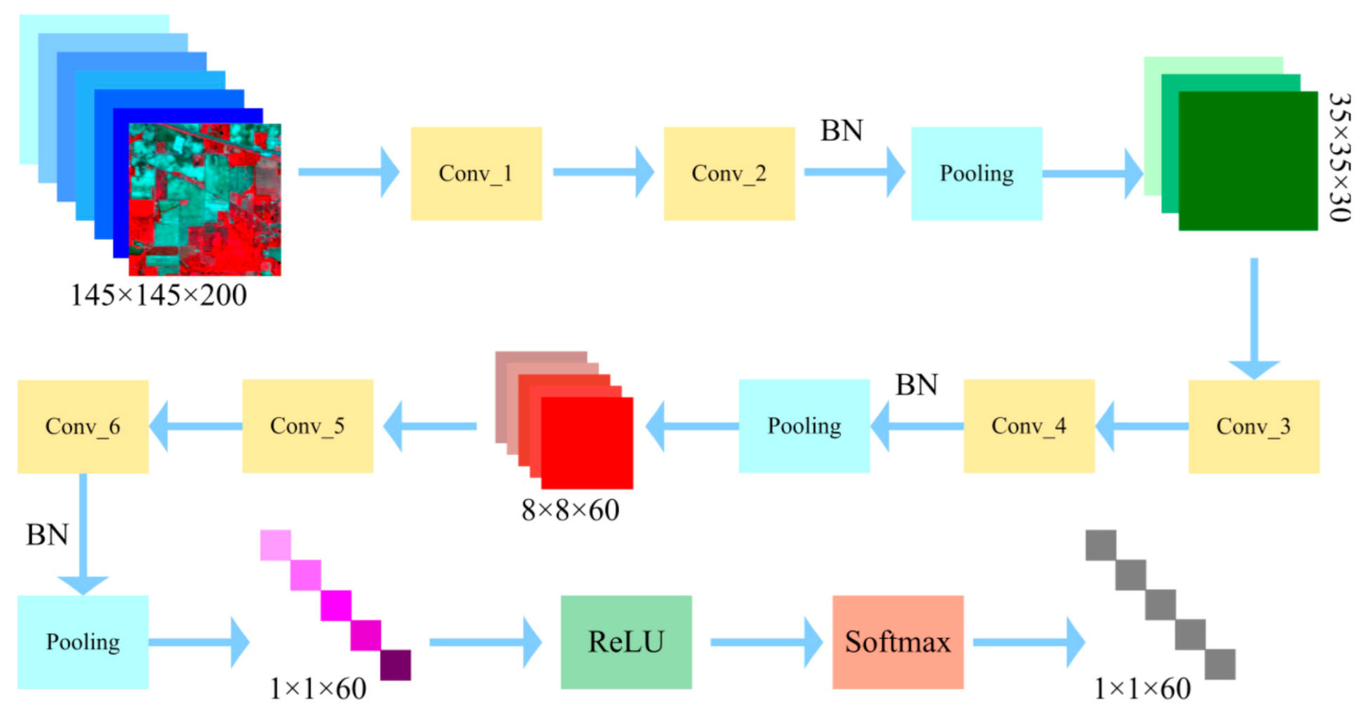
The visualization of the down-sampling process in the proposed scheme is shown in Figure 2. The main spectral features can be extracted from the original HSI by using different kernel sizes and different number of convolutional kernels. Table 1 lists the size and the number of convolutional kernels, stride and output size of the feature map.
2.2. Deconvolution and Unpooling
It is well known that the main features of the image can be effectively extracted by using the down-sampling technique with multiple convolutional kernels. If the whole image is taken as the classification object, this obviously helps to improve the final classification result. However, this is not enough for the HSI classification because an HSI often contains numerous pixels belonging to different classes. In addition, spatial structure information of the image is gradually lost as the number of convolution layers and pooling layer increases. Previous work demonstrates that in the process of HSI classification, satisfactory classification results are usually not obtained if only considering the spectral information of an HSI. To address this problem, deconvolution (also known as transposed convolution) and unpooling technique are used to restore the spatial structure of feature map and to retrieve the missing image details.
Deconvolution is a transformation process used to reverse the effect of convolution on recorded data, which has been widely used in signal processing and image processing. In the convolutional layer, we expand the input matrix and the output matrix into column vectors X and Y, respectively. For a given convolution kernel K, the sparse matrix C can be derived, such that
Deconvolution is to carry on the inverse operation to the above transformation Equation (4), that is, through the matrix C and vector Y to get X. According to the sizes of the feature map and the convolution kernel, one can easily obtain the following deconvolution operation
The deconvolution operation, however, only restores the size of the matrix X rather than each element value. In the traditional upsampling process, the interpolation or resampling techniques are commonly used to generate smooth images, such as nearest neighbor interpolation, bilinear interpolation, cubic convolution interpolation [52,53,54]. These techniques rescale the image to a specific size and replenish the information of each pixel. However, the interpolation-based method blurs the boundary of the class when smoothing the data. Unlike interpolation and resampling approaches, unpooling is the reverse operation of the max pooling. Unpooling is to replenish 0 at all positions in unpooling layers, except for the maximum feature. Thus, the spatial structure information of maximum is well preserved.
After the downsampling network, a multi-scale upsampling feature recovery scheme is adopted in the proposed SP-CNN framework, as shown in Figure 1. Corresponding to the downsampling process, each upsampling block also consists of two deconvolutional layers and an unpooling layer, and is accompanied by a batch normalization layer and a rectified linear unit layer. Furthermore, each upsampling block corresponds to a downsampling block.
2.3. Superpixel Pooling
The commonly used CNN-based HSI classification methods convert the features extracted from the last network layer into a one-dimensional vectors through global maximum pooling or global average pooling. Then, a fully connected neural network is utilized to classify the obtained vectors at pixel-level by activating the learned features. For this HSI classification framework, there are several issues to be further considered: (i) a large number of training samples are needed to train classifiers with high accuracy. However, the acquisition of labeled samples is usually expensive; (ii) the boundary and regional shape information of geographic objects are gradually lost after continuous downsampling. This will undoubtedly affect the final classification results. To address these issues, we design a superpixel pooling layer before classifier, as shown in Figure 1.
In this study, we adopt the graph-based ERS approach to segment the HSIs into superpixels, due to its advantages of fast implementation and good edge retention [25]. Since ERS was originally designed for image segmentation, it is necessary to execute principal component analysis (PCA) algorithm in advance to reduce the dimension of high-dimensional HSIs. We herein take the first principal component to generate the base image because it contains the primary information of the raw data.
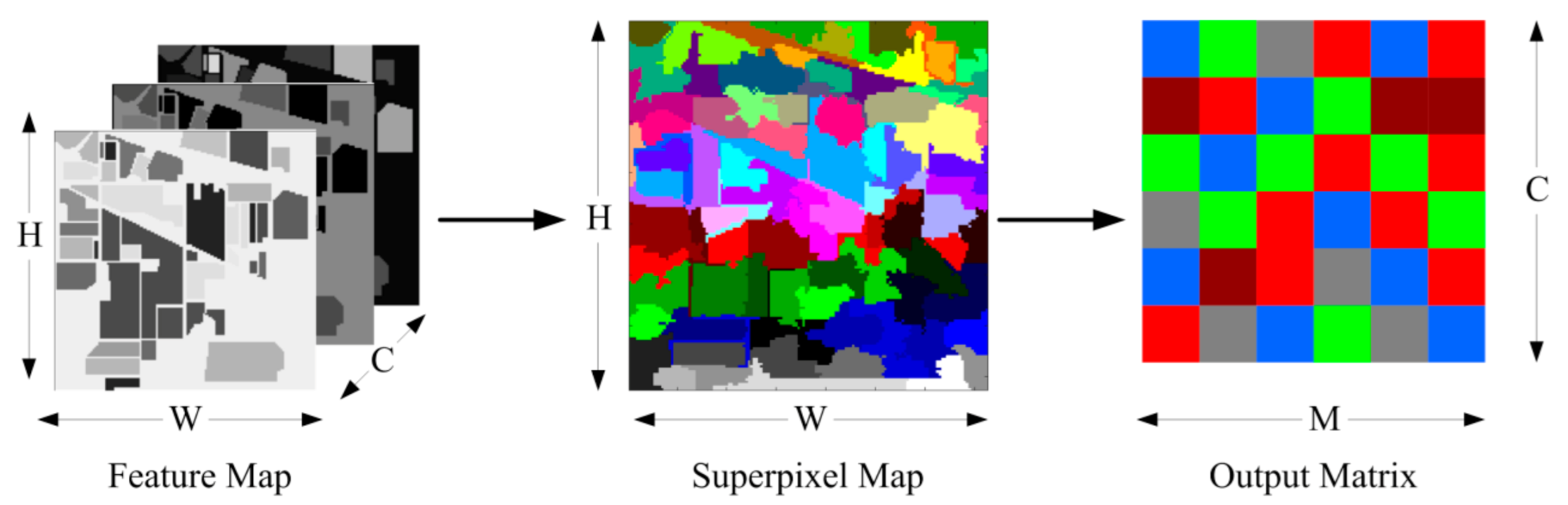
The homogeneity of superpixels implies that pixels in the same superpixel should belong to the same class with higher probability. Therefore, it is reasonable to take superpixels as a whole in the classification process. This will greatly reduce the number of samples to be classified. Additionally, the feature of adaptive size and shape of superpixel are more conducive to maintaining spatial structure information of the HSIs. The designed superpixel pooling layer is illustrated in Figure 3.
Suppose that the feature map is input into the superpixel pooling layer, where W represents the width, H the height and C the number of channels; the HSIs with size of W × H is divided into M superpixels, and each superpixel contains ni pixels. The output of superpixel pooling layer is a matrix, denoted by . The pooling function is defined as
where is the arithmetic mean of the mean and the median of the j-th channel of the ni pixels in the superpixel . The median vector used in Equation(6) is an attempt to reduce the effect of singular values on this function.
In the superpixel pooling layer, taking each superpixel instead of the pixel as input to the neural network has the advantages of (i) effective fusion of main spectral features learned from downsampling and spatial structure information provided by superpixels, (ii) preservation of spatial information in original HSIs, and (iii) effective reduction of samples to be classified. Particularly, the third advantage also means that the proportion of labeled samples increases. In other words, the adoption of superpixel pooling weakens the dependence of our proposal on massive training samples. In addition, different from traditional pooling layer, superpixel pooling does not require a pre-designed rectangular layout.
2.4. Transfer Learning between HSIs
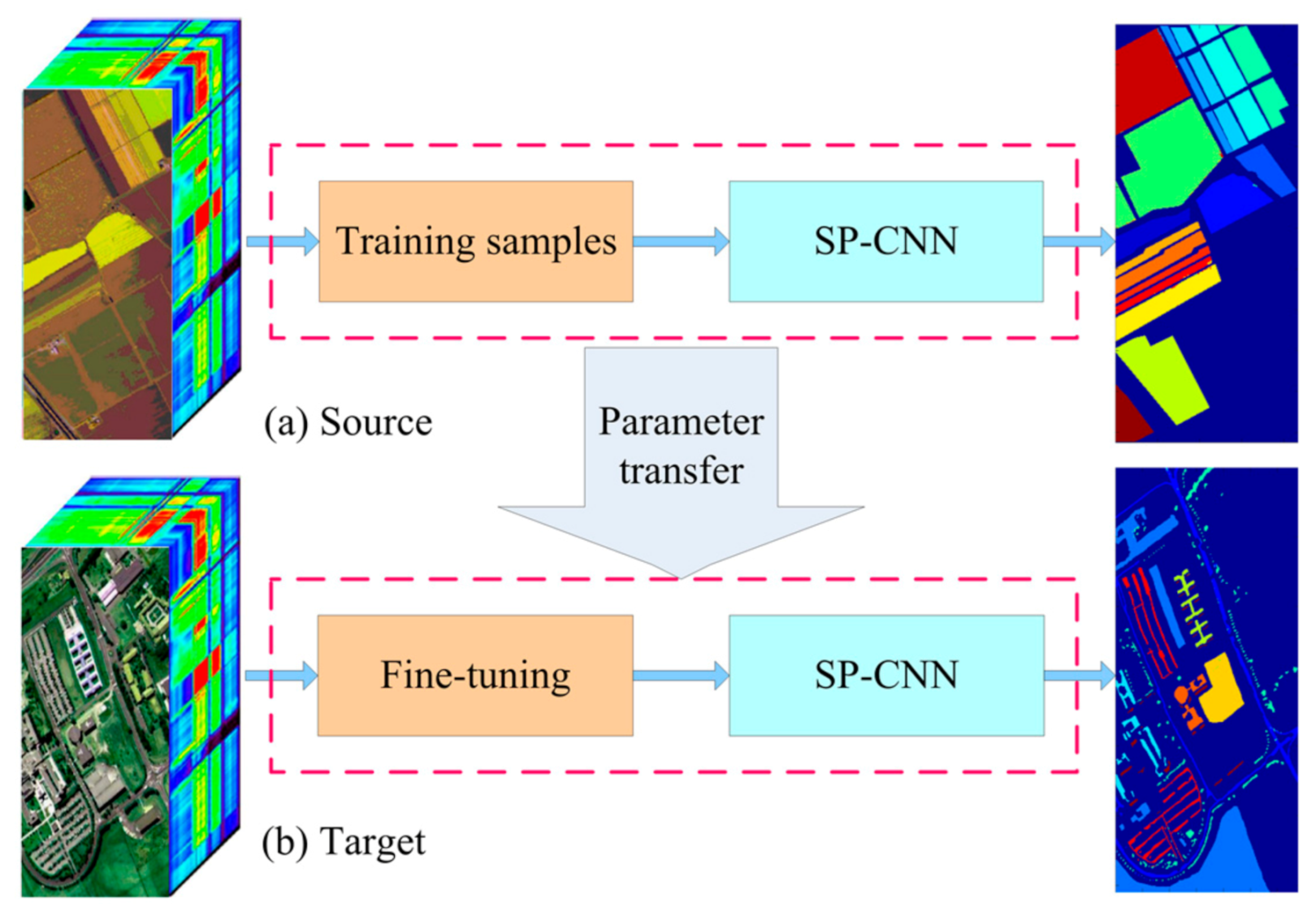
To improve the training efficiency and the classification performance of deep learning model with limited labeled samples, we apply transfer learning technique to the proposed SP-CNN framework. It is well known that the excellent classification performance of deep learning-based methods depends on the massive parameters and plenty of labeled samples to balance the final classification results. This means that we need a long time to train the designed model. Transfer learning can accelerate training process by transferring well-trained parameters from the source domain to the target. In addition, the use of superpixel pooling technique can effectively alleviate the problem which there are insufficient training samples on both resource and target datasets. Figure 4 shows that, transfer learning is composed of two parts: source and target. Specifically, the SP-CNN was first pre-trained on the source HSI, and then it was fine-tuned on the target HSI by using fewer samples. As the pre-trained model has already been very robust, new tasks can be rapidly accomplished by setting a subtle learning rate.
3. Experimental Results and Analysis
To verify the effectiveness of the proposed SP-CNN method, extensive experiments were conducted on three public hyperspectral datasets, namely, Indian Pines, Pavia University and Salinas. These three typical benchmarks are widely utilized to test the performance of the HSI classification algorithms.
3.1. Datasets and Evaluation Indicators
Indian Pines dataset was collected by an airborne visible infrared imaging spectrometer (AVIRIS) sensor in a pine field in the northwestern Indiana. This image consists of 16 different categories, 145 × 145 pixels, and 200 bands. After removing background points, there are 10,249 pixels to be classified. The imbalance between class sizes leads to the difficulty of accurate classification.
Pavia University image was acquired by reflective optics system imaging spectrometer (ROSIS) sensors at University of Pavia, Italy. It has nine classes, 610 × 340 pixels, and 103 bands. The spatial structure of each class in this dataset varies greatly, which brings great challenges to classification.
The last dataset is the Salinas dataset. This dataset was collected by AVIRIS sensor from the Salinas Valley in California. It is composed of 16 categories, 512 × 217 pixels, and 204 bands. In this image, there are two spatially adjacent classes whose spectra are very similar.
In all experiments conducted in this work, the classification results were evaluated by adopting three commonly used indices, that is, overall accuracy (OA), average accuracy (AA), and kappa coefficient (κ). To overcome the classification bias caused by random marking, the mean and standard deviation of 10 independent runs were calculated as the final classification results.
3.2. Classification Results and Analysis
The suggested method was compared with the other four state-of-the-art HSI classification approaches, namely, artificial neural network (ANN), CNN [55], convolutional recurrent neural network (CRNN) [56], CNN based on pixel-pair features (CNN-PPF) [57], spectral-spatial CNN (SS-CNN) [58], because these methods are based on CNN framework [56,57,58] and adopt ANN as the final classifier. Table 2, Table 3 and Table 4 list the comparison results of these algorithms on the three datasets.
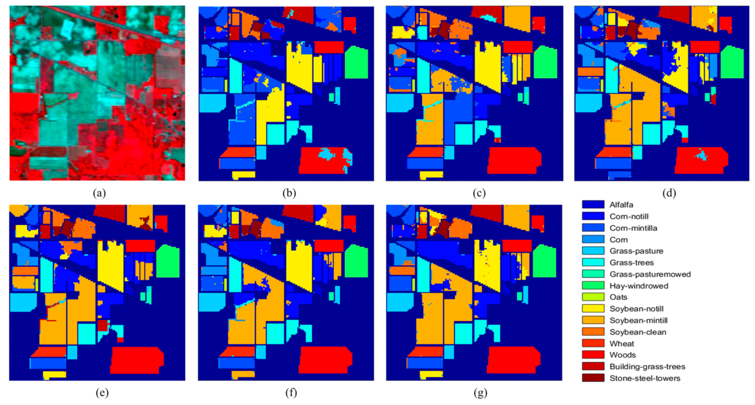
The classification results of several competitive algorithms on Indian Pines dataset are reported in Table 2. Compared with SS-CNN, the classification accuracy of our method achieves 94.45%, which is about 10% higher (94.45% vs. 84.58%). The SS-CNN method is superior to CRNN and CNN approaches, due to the use of spatial information in classification. CNN, CRNN, SS-CNN and SP-CNN methods outperform ANN because the CNN-based framework can extract the main spectral features from raw data. Satisfactory results on this dataset are not obtained by CNN, CRNN and SS-CNN when there are no more than 30 labeled pixels per class. However, these three methods can still exhibit superior classification performance in the case of 200 labeled pixels per class [55,56,58]. Noted that in this case, seven classes with no more than 400 pixels per class were ignored in the classification. Experimental results of this image demonstrate that the proposed SP-CNN method can classify the unbalanced dataset with limited labeled samples. The classification result maps of these methods are shown in Figure 5.
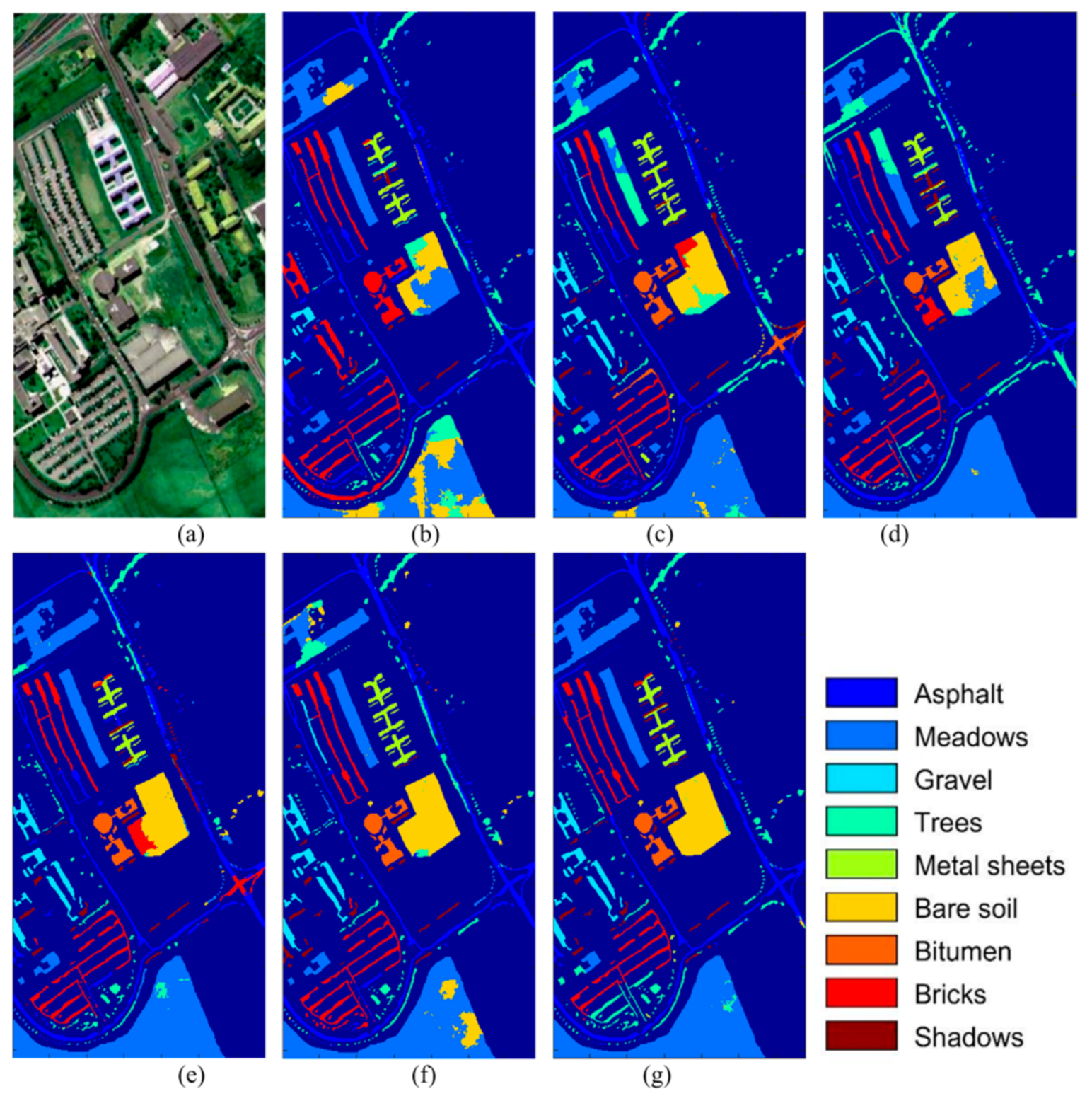
The classification statistics of six methods on Pavia University dataset are listed in Table 3. According to the values of three evaluation indicators, our method has defeated the other five algorithms. The utilization of spatial information in classification makes the classification results of SS-CNN and SP-CNN methods better than those of other four approaches. The suggested classification scheme, however, does not identify classes “Trees” and “Shadows” well from other ground objects. This may be because, after removing the background points, fragmented or strip-like class distributions result in the generation of many superpixels with very small size, thus weakening the role of spatial structure information in classification. Particularly for class “Trees”, the spectral-based classifiers, ANN, CNN and CRNN also do not achieve good classification accuracy. This shows that the spectrum of this class is complex. Although good classification results can be obtained by marking more pixels in each class, it is worth studying how to improve the recognition accuracy of this class under the deep learning framework in the case of limited labeled samples. Figure 6 presents the visualization of the classification results in Table 3.
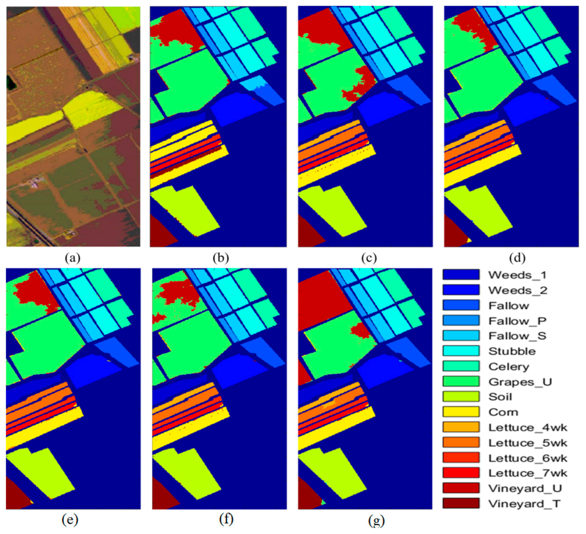
Table 4 summarizes the classification results of six classifiers on Salinas dataset. The main challenge for this dataset is to classify classes “Grapes_U” and “Vineyard_U” correctly, because there is a slight spectral difference between these two spatially adjacent categories. It can be seen from Table 4, none of the six methods has satisfactory classification accuracy for class “Vineyard_U”. As shown in Figure 7c–e, most of pixels of class “Vineyard_U” were misclassified and incorrectly assigned to the class “Grapes_U”, especially for the classifiers ANN and CNN. As was expected, three spectral-spatial classifiers, CNN-PPF, SS-CNN and SP-CNN show good classification completion and achieve more than 90% classification accuracy.
4. Parametric Analysis
In this section, we analyze the influence of the number of training samples on classification results, the comparison of the running time of six classifiers and the impact of transfer learning on the efficiency of the proposed method, respectively. All experiments were carried out on the computer with Intel i3 9100F CPU, 16GB Memory and NVIDIA GEFORCE RTX 1660 GPU.
4.1. Impact of Different Labeled Samples on Classification Results
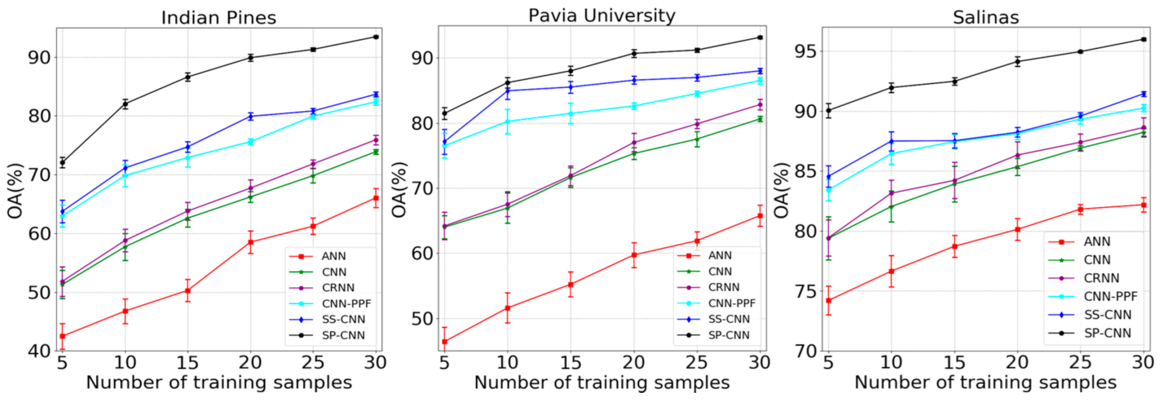
To further demonstrate the advantage of the framework, we compare the proposed classification framework with five other competitors for different numbers of training samples (per class) on three datasets. As the number of training samples increases, the classification results of six methods are obviously getting better and better (Figure 8). The main reason should be that with the increase of the number of training samples, the initial parameter values gradually approximate the optimal values in the training process. As a result, the classification ability of these classifiers is enhanced and satisfactory classification results are obtained. For our method, the number of marked superpixels may be smaller than the number of marked pixels, because it is possible that multiple labeled pixels are in the same superpixel block. In addition, our method is still superior to the other five classification algorithms on three datasets. In particular, there is a about 10% and 5% gap between the remaining classifiers and our proposal on Indian Pines and Salinas images, respectively. This indicates the necessity of inserting a superpixel pooling layer to the proposed framework. As expected, three CNN-based spectral-spatial classifiers, CNN-PPF, SS-CNN and SP-CNN, outperform the spectral classification methods of ANN, CNN and CRNN. It shows that the use of spatial information can improve classification results. As seen from Figure 8, the classification accuracy of our method on three datasets exceeds 90% when marking 20 pixels per class. This means the effectiveness of the scheme in the case of limited labeled pixels.
4.2. Running Times
Running time is another important statistics to evaluate the effectiveness of HSI classification algorithm. An effective and efficient classification algorithm means that it may be applied in engineering field. Table 5 reports the running times of six HSI classification algorithms on three images. The structure of neural network in CNN-based methods is the same as that adopted in ANN. The running time of CNN is less than ANN because the main spectral features, instead of original spectral information are fed into the neural network. The use of recurrent technique in ANN results in an increase of computing time of CRNN. Since CNN-PPF method takes more time to calculate the pixel-pair model, it is more time-consuming. Compared with the other five methods, our method is time-saving. This should benefit from the adoption of transfer learning strategy and the smaller data size of the input network layer in our method.
4.3. Influence of the Number of Superpixels
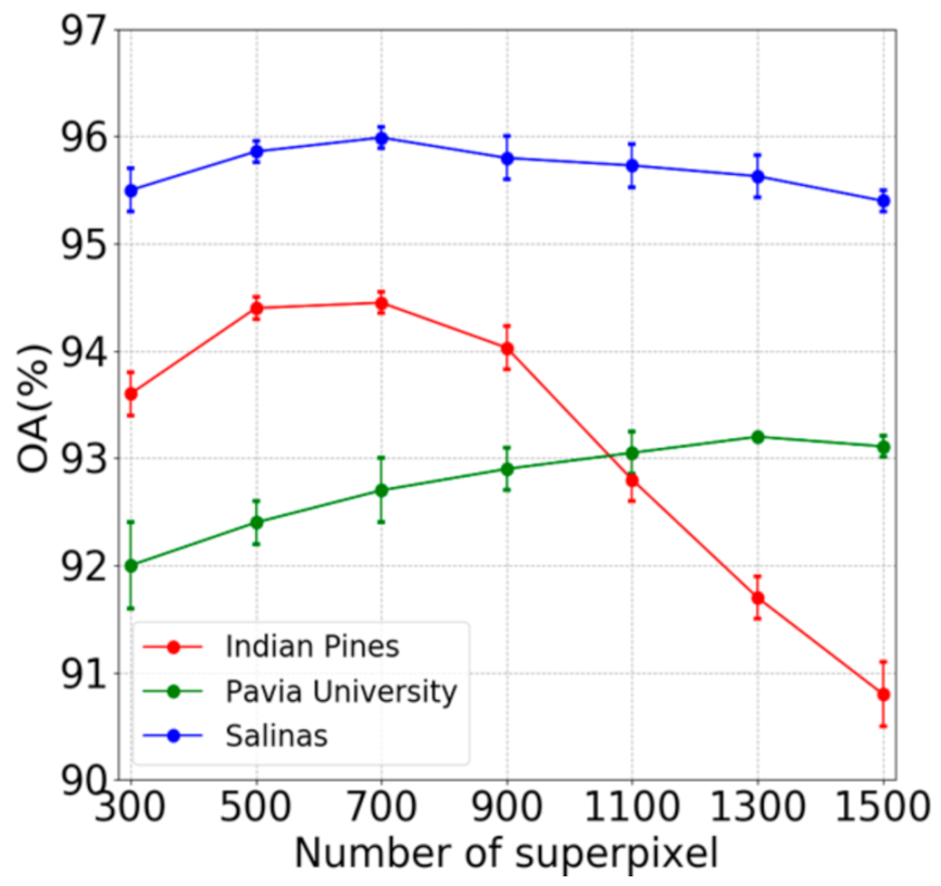
Another factor that affects classification results of our method is the number of superpixel. Thus, far, the determination of the optimal number of superpixels still depends on the experimental results. Figure 9 presents the change of the classification results of our method with the increase of superpixel number on three datasets. There is a change of about 1% on Pavia University and Salinas images when the number of superpixel increases from 300 to 1500. This indicates that the proposed algorithm is relatively robust on these two datasets. When the number of superpixels is more than 700, the classification results of Indian Pines image decrease sharply (about 4%). This may be due to the unbalanced characterictic of the dataset and the small superpixel volume, which result in the increase of the misclassification of the superpixels. Based on the experiments, in this work, the number of superpixel is 700, 1300 and 700 for Indian Pines, Pavia University andSalinas images, respectively.
4.4. Impact of Network Architecture and Transfer Learning on Efficiency
Generally, the increase of convolution layers means that the extracted spectral information will be more accurate. However, this will take more computational time since more parameters are involved. Table 6 lists the classification results and the running times of the proposed SP-CNN method for different numbers of convolution layers on three images. In Table 6, SP-CNN-4 represents that there are four convolutional layers, two pooling layers, one superpixel pooling layer and one fully connected layer in the proposed framework. With the increase of network depth, the number of used parameters and computational time show an obvious growth trend. However, the improvement of classification results is slow and insignificant. According to the classification results and running time. A six-layer structure is adopted in the framework to avoid over-fitting and gradient problems.
For the pre-specified classification accuracy, Table 7 shows the effect of transfer learning on training efficiency of the suggested SP-CNN method. The training times of SP-CNN on three datasets are reported in the second column without using transfer learning. If Indian Pines, Pavia University and Salinas images are, respectively, taken as the source domain (pre-training model) and the remaining two images as the target, the training times of SP-CNN on the other two datasets are listed in columns 3 to 5. When the parameters well-trained on the University of Pavia images are transferred to the model that classifies Salinas image, or versa, the fourth and fifth columns show that the training time of SP-CNN on the target dataset is significantly reduced. However, the opposite conclusion is obtained while Indian Pines image acts as the target dataset. It is probably because, unlike the other two images, Indian Pines image is an unbalanced dataset. This makes the well-trained parameters on the other two datasets unsuitable for the dataset.
5. Conclusions
In this work, we suggest a spectral-spatial deep learning model for HSI classification based on CNN and superpixel. Different from the traditional CNN structure, an up-sampling process is connected after down-sampling to recover the lost spatial structure information while preserving the extracted spectral features. The extracted spectral features and spatial structure information provided by superpixel are effectively fused in the designed superpixel pooling layer. Furthermore, the homogeneity of superpixels allows to regard each superpixel instead of a pixel as the basic input of classifier, thus reducing the number of objects to be classified. For a fixed number of training samples, the reduction of the object to be classified means an increase in the proportion of training samples. This is the main reason why the proposed SP-CNN method can effectively classify the HSI with limited training samples. At the same time, this idea may serve as a feasible solution to the problem that the CNN-based HSI classification framework cannot achieve better classification accuracy due to insufficient training samples. As with the traditional CNN classification framework, the efficiency of the proposed SP-CNN method relies on the optimization process of a large number of parameters. As expected, the use of transfer learning technique in the proposed model significantly shortens the training time. Therefore, this method can be applied to solve other practical problems in the field of remote sensing. As our work effectively integrates the advantages of CNN architecture, superpixel and transfer learning, the proposed SP-CNN method can classify the hyperspectral data with a small number of training samples accurately and quickly. Extensive experimental and comparative results on three benchmarks confirm the effectiveness and efficiency of the SP-CCN.
Thus far, the optimal superpixel segmentation scale is still an experimental result and is difficult to specify in advance. In the future, we would like to adopt the superpixel merging technique to alleviate the dependence of the superpixel-level classification method on the segmentation scale.
Author Contributions
F.X. and Q.G. conceived and designed the experiments; Q.G. performed the experiments; F.Z. and C.J. analyzed the data and developed the figures and tables; F.X., Q.G. and C.J. wrote the paper. All authors have read and agreed to the published version of the manuscript.
Funding
This research was funded by the National Natural Science Foundation of China (Grants number 41801340); Natural Science Research Project of Liaoning Education Department (Grants number LJ2019013), andthe APC was funded by the National Natural Science Foundation of China (Grants number 41801340).
Acknowledgments
We would like to thank the authors of CRNN, CNN-PPF, and SS-CNN for sharing the source code.
Conflicts of Interest
The authors declare no conflict of interest.
References
- Mukherjee, F.; Singh, D. Assessing Land Use–Land Cover Change and Its Impact on Land Surface Temperature Using LANDSAT Data: A Comparison of Two Urban Areas in India. Earth Syst. Environ. 2020, 4, 385–407. [Google Scholar] [CrossRef]
- Abdelmoneim, H.; Soliman, M.; Moghazy, H. Evaluation of TRMM 3B42V7 and CHIRPS Satellite Precipitation Products as an Input for Hydrological Model over Eastern Nile Basin. Earth Syst. Environ. 2020, 4, 685–698. [Google Scholar] [CrossRef]
- Irteza, S.; Nichol, J.; Shi, W.; Abbas, S. NDVI and Fluorescence Indicators of Seasonal and Structural Changes in a Tropical Forest Succession. Earth Syst. Environ. 2021, 5, 127–133. [Google Scholar] [CrossRef]
- Stuart, M.; Stanger, L.; Hobbs, M.; Pering, T.; Thio, D.; McGonigle, A.; Willmott, J. Low-Cost Hyperspectral Imaging System: Design and Testing for Laboratory-Based Environmental Applications. Sensors 2020, 20, 3293. [Google Scholar] [CrossRef] [PubMed]
- Park, S.; Song, A. Discrepancy Analysis for Detecting Candidate Parcels Requiring Update of Land Category in Cadastral Map Using Hyperspectral UAV Images: A Case Study in Jeonju, South Korea. Remote Sens. 2020, 12, 354. [Google Scholar] [CrossRef] [Green Version]
- Li, Z.; Ling, Q.; Wu, J.; Wang, Z.; Lin, Z. A Constrained Sparse-Representation-Based Spatio-Temporal Anomaly Detector for Moving Targets in Hyperspectral Imagery Sequences. Remote Sens. 2020, 12, 2783. [Google Scholar] [CrossRef]
- Cerreta, M.; Mele, R.; Poli, G. Urban Ecosystem Services (UES) Assessment within a 3D Virtual Environment: A Methodological Approach for the Larger Urban Zones (LUZ) of Naples, Italy. Appl. Sci. 2020, 10, 6205. [Google Scholar] [CrossRef]
- Faqeerzada, M.; Perez, M.; Lohumi, S.; Lee, H.; Kim, G.; Wakholi, C.; Joshi, R.; Cho, B. Online Application of a Hyperspectral Imaging System for the Sorting of Adulterated Almonds. Appl. Sci. 2020, 10, 6569. [Google Scholar] [CrossRef]
- Lim, H.; Lee, O.; Shung, K.; Kim, J.; Kim, H. Classification of Breast Cancer Cells Using the Integration of High-Frequency Single-Beam Acoustic Tweezers and Convolutional Neural Networks. Cancers 2020, 12, 1212. [Google Scholar] [CrossRef]
- Gorban, A.; Mirkes, E.; Tukin, I. How deep should be the depth of convolutional neural networks: A backyard dog case study. Cogn. Comput. 2020, 12, 388. [Google Scholar] [CrossRef] [Green Version]
- Chen, Y.; Lei, T.; Yao, S.; Wang, H. PM2.5 Prediction Model Based on Combinational Hammerstein Recurrent Neural Networks. Mathematics 2020, 8, 2178. [Google Scholar] [CrossRef]
- Ince, I. Performance Boosting of Scale and Rotation Invariant Human Activity Recognition (HAR) with LSTM Networks Using Low Dimensional 3D Posture Data in Egocentric Coordinates. Appl. Sci. 2020, 10, 8474. [Google Scholar] [CrossRef]
- Wang, F.; Leng, L.; Teoh, A.; Chu, J. Palmprint False Acceptance Attack with a Generative Adversarial Network (GAN). Appl. Sci. 2020, 10, 8547. [Google Scholar] [CrossRef]
- Wang, G.; Ren, P. Hyperspectral Image Classification with Feature-Oriented Adversarial Active Learning. Remote Sens. 2020, 12, 3879. [Google Scholar] [CrossRef]
- Qiu, T.; Liu, M.; Zhou, G.; Wang, L.; Gao, K. An Unsupervised Classification Method for Flame Image of Pulverized Coal Combustion Based on Convolutional Auto-Encoder and Hidden Markov Model. Energies 2019, 12, 2585. [Google Scholar] [CrossRef] [Green Version]
- Chien, Y.; Hsu, K.; Tsao, H. Phonocardiography Signals Compression with Deep Convolutional Autoencoder for Telecare Applications. Appl. Sci. 2020, 10, 5842. [Google Scholar] [CrossRef]
- Li, Y.; Chen, R.; Zhang, Y.; Zhang, M.; Chen, L. Multi-Label Remote Sensing Image Scene Classification by Combining a Convolutional Neural Network and a Graph Neural Network. Remote Sens. 2020, 12, 4003. [Google Scholar] [CrossRef]
- Gao, Q.; Lim, S.; Jia, X. Hyperspectral Image Classification Using Convolutional Neural Networks and Multiple Feature Learning. Remote Sens. 2018, 10, 299. [Google Scholar] [CrossRef] [Green Version]
- Acquarelli, J.; Marchiori, E.; Buydens, L.M.; Tran, T.; Van, T. Spectral-Spatial Classification of Hyperspectral Images: Three Tricks and a New Learning Setting. Remote Sens. 2018, 10, 1156. [Google Scholar] [CrossRef] [Green Version]
- Cao, J.; Chen, Z.; Wang, B. Deep Convolutional networks with superpixel segmentation for hyperspectral image classification. In Proceedings of the 2015 IEEE International Geoscience and Remote Sensing Symposium (IGARSS), Beijing, China, 10–15 July 2016; pp. 3310–3313. [Google Scholar]
- Li, Z.; Guo, F.; Li, Q.; Ren, G.; Wang, L. An Encoder–Decoder Convolution Network With Fine-Grained Spatial Information for Hyperspectral Images Classification. IEEE Access 2020, 8, 33600. [Google Scholar] [CrossRef]
- Wang, Z.; Xia, Q.; Yan, J.; Xuan, S.; Yang, C. Hyperspectral Image Classification Based on Spectral and Spatial Information Using Multi-Scale ResNet. Appl. Sci. 2019, 9, 4890. [Google Scholar] [CrossRef] [Green Version]
- Tao, C.; Pan, H.; Li, Y.; Zou, Z. Unsupervised Spectral-Spatial Feature Learning With Stacked Sparse Autoencoder for Hyperspectral Imagery Classification. IEEE Geosci. Remote Sens. Lett. 2015, 12, 2438. [Google Scholar]
- Wang, C.; Zhang, L.; Wei, W.; Zhang, Y. When Low Rank Representation Based Hyperspectral Imagery Classification Meets Segmented Stacked Denoising Auto-Encoder Based Spatial-Spectral Feature. Remote Sens. 2018, 10, 284. [Google Scholar] [CrossRef] [Green Version]
- Liu, M.; Tuzel, O.; Ramalingam, S.; Chellappa, R. Entropy rate superpixel segmentation. In Proceedings of the IEEE Conference on Computer Vision and Pattern Recognition (CVPR), Colorado Springs, CO, USA, 20–25 June 2011; pp. 2097–2104. [Google Scholar]
- Achanta, R.; Shaji, A.; Smith, K.; Lucchi, A.; Fua, P.; Süsstrunk, S. SLIC superpixels compared to state-of-the-art superpixel methods. IEEE Trans. Pattern Anal. Mach. Intell. 2012, 34, 2274–2282. [Google Scholar] [CrossRef] [PubMed] [Green Version]
- Alkhatib, M.Q.; Velez-Reyes, M. Improved Spatial-Spectral Superpixel Hyperspectral Unmixing. Remote Sens. 2019, 11, 2374. [Google Scholar] [CrossRef] [Green Version]
- Zhang, Y.; Jiang, X.; Wang, X.; Cai, Z. Spectral-Spatial Hyperspectral Image Classification with Superpixel Pattern and Extreme Learning Machine. Remote Sens. 2019, 11, 1983. [Google Scholar] [CrossRef] [Green Version]
- Liu, Y.; Condessa, F.; Bioucas-Dias, J.M.; Du, P.; Plaza, A. Convex Formulation for Multiband Image Classification With Superpixel-Based Spatial Regularization. IEEE Trans. Geosci. Remote Sens. 2018, 56, 2704–2721. [Google Scholar] [CrossRef]
- Farooq, A.; Jia, X.; Hu, J.; Zhou, J. Multi-Resolution Weed Classification via Convolutional Neural Network and Superpixel Based Local Binary Pattern Using Remote Sensing Images. Remote Sens. 2019, 11, 1692. [Google Scholar] [CrossRef] [Green Version]
- Xie, F.; Lei, C.; Jin, C.; An, N. A Novel Spectral–Spatial Classification Method for Hyperspectral Image at Superpixel Level. Appl. Sci. 2020, 10, 463. [Google Scholar] [CrossRef] [Green Version]
- Zhao, Y.; Su, F.; Yan, F. Novel Semi-Supervised Hyperspectral Image Classification Based on a Superpixel Graph and Discrete Potential Method. Remote Sens. 2020, 12, 1528. [Google Scholar] [CrossRef]
- Jiang, J.; Ma, J.; Chen, C.; Wang, Z.; Cai, Z.; Wang, L. SuperPCA: A Superpixelwise PCA Approach for Unsupervised Feature Extraction of Hyperspectral Imagery. IEEE Trans. Geosci. Remote Sens. 2018, 56, 4581. [Google Scholar] [CrossRef] [Green Version]
- Xu, H.; Zhang, H.; He, W.; Zhang, L. Superpixel-based spatial-spectral dimension reduction for hyperspectral imagery classification. Neurocomputing 2019, 360, 138. [Google Scholar] [CrossRef]
- Zhang, L.; Su, H.; Shen, J. Hyperspectral Dimensionality Reduction Based on Multiscale Superpixelwise Kernel Principal Component Analysis. Remote Sens. 2019, 11, 1219. [Google Scholar] [CrossRef] [Green Version]
- Blanco, S.; Heras, D.; Argüello, F. Texture Extraction Techniques for the Classification of Vegetation Species in Hyperspectral Imagery: Bag of Words Approach Based on Superpixels. Remote Sens. 2020, 12, 2633. [Google Scholar] [CrossRef]
- Liu, B.; Wei, Y.; Zhang, Y.; Yang, Q. Deep neural networks for high dimension, low sample size data. In Proceedings of the 21 International Joint Conference on Artificial Intelligence (IJCAI), Melbourne, Australia, 19–25 August 2017; pp. 2287–2293. [Google Scholar]
- Makantasis, K.; Karantzalos, K.; Doulamis, A.; Doulamis, N. Deep supervised learning for hyperspectral data classification through convolutional neural networks. In Proceedings of the 2015 IEEE International Geoscience and Remote Sensing Symposium (IGARSS), Milan, Italy, 26–31 July 2015; pp. 4959–4962. [Google Scholar]
- Zhang, H.; Li, Y.; Zhang, Y.; Shen, Q. Spectral-spatial classification of hyperspectral imagery using a dualchannel convolutional neural network. Remote Sens. Lett. 2017, 8, 438–447. [Google Scholar] [CrossRef] [Green Version]
- Li, W.; Chen, C.; Zhang, M.; Li, H.; Du, Q. Data Augmentation for Hyperspectral Image Classification With Deep CNN. IEEE Geosci. Remote Sens. Lett. 2018, 16, 593–597. [Google Scholar] [CrossRef]
- Cui, B.; Xie, X.; Hao, S.; Cui, J.; Lu, Y. Semi-Supervised Classification of Hyperspectral Images Based on Extended Label Propagation and Rolling Guidance Filtering. Remote Sens. 2018, 10, 515. [Google Scholar] [CrossRef] [Green Version]
- Amirabbas, D.; Erchan, A.; Berrin, Y.; Andreas, M.; Christian, R. GMM-Based Synthetic Samples for Classification of Hyperspectral Images With Limited Training Data. IEEE Geosci. Remote Sens. Lett. 2018, 15, 942–946. [Google Scholar]
- Rao, M.; Tang, P.; Zhang, Z. Spatial–Spectral Relation Network for Hyperspectral Image Classification with Limited Training Samples. IEEE J. Sel. Top. Appl. Earth Obs. Remote Sens. 2019, 99, 1–15. [Google Scholar] [CrossRef]
- Xie, F.; Hu, D.; Li, F.; Yang, J.; Liu, D. Semi-Supervised Classification for Hyperspectral Images Based on Multiple Classifiers and Relaxation Strategy. ISPRS Int. J. Geo-Inf. 2018, 7, 284. [Google Scholar] [CrossRef] [Green Version]
- Acción, Á.; Argüello, F.; Heras, D. Dual-Window Superpixel Data Augmentation for Hyperspectral Image Classification. Appl. Sci. 2020, 10, 8833. [Google Scholar] [CrossRef]
- Yang, J.; Zhao, Y.; Chan, J. Learning and transferring deep joint spectral–spatial features for hyperspectral classification. IEEE Trans. Geosci. Remote Sens. 2017, 55, 4729–4742. [Google Scholar] [CrossRef]
- Liu, X.; Sun, Q.; Meng, Y.; Fu, M.; Bourennane, S. Hyperspectral image classification based on parameter-optimized 3D-CNNs combined with transfer learning and virtual samples. Remote Sens. 2018, 10, 1425. [Google Scholar] [CrossRef] [Green Version]
- Jiang, Y.; Li, Y.; Zhang, H. Hyperspectral image classification based on 3-D separable ResNet and transfer learning. IEEE Geosci. Remote Sens. Lett. 2019, 16, 1949–1953. [Google Scholar] [CrossRef]
- He, X.; Chen, Y.; Ghamisi, P. Heterogeneous transfer learning for hyperspectral image classification based on convolutional neural network. IEEE Trans. Geosci. Remote Sens. 2019, 58, 3246–3263. [Google Scholar] [CrossRef]
- Zhao, X.; Liang, Y.; Guo, A.J.; Zhu, F. Classification of small-scale hyperspectral images with multi-source deep transfer learning. Remote Sens. Lett. 2020, 11, 303–312. [Google Scholar] [CrossRef]
- Zhang, H.; Li, Y.; Jiang, Y.; Wang, P.; Shen, Q.; Shen, C. Hyperspectral classification based on lightweight 3-D-CNN with transfer learning. IEEE Trans. Geosci. Remote Sens. 2019, 57, 5813–5828. [Google Scholar] [CrossRef] [Green Version]
- Jiang, N.; Wang, L. Quantum image scaling using nearest neighbor interpolation. Quantum Inf. Process. 2015, 14, 1559–1571. [Google Scholar] [CrossRef]
- Jawak, S.; Luis, A. A Comprehensive Evaluation of PAN-Sharpening Algorithms Coupled with Resampling Methods for Image Synthesis of Very High Resolution Remotely Sensed Satellite Data. Adv. Remote Sens. 2013, 2, 40777. [Google Scholar] [CrossRef] [Green Version]
- Keys, R. Cubic convolution interpolation for digital image processing. IEEE Trans. Acoustics. Speech. Signal. Process. 2003, 29, 1153–1160. [Google Scholar] [CrossRef] [Green Version]
- Hu, W.; Huang, Y.; Wei, L.; Zhang, F.; Li, H. Deep Convolutional Neural Networks for Hyperspectral Image Classification. J. Sens. 2015, 2015, 258619. [Google Scholar] [CrossRef] [Green Version]
- Wu, H.; Prasad, S. Convolutional Recurrent Neural Networks for Hyperspectral Data Classification. Remote Sens. 2017, 9, 298. [Google Scholar] [CrossRef] [Green Version]
- Li, W.; Wu, G.; Zhang, F.; Du, Q. Hyperspectral Image Classification Using Deep Pixel-Pair Features. IEEE Trans. Geosci. Remote Sens. 2016, 55, 844–853. [Google Scholar] [CrossRef]
- Mei, S.; Ji, J.; Hou, J.; Xu, L.; Qian, D. Learning Sensor-Specific Spatial-Spectral Features of Hyperspectral Images via Convolutional Neural Networks. IEEE Trans. Geosci. Remote Sens. 2017, 55, 4520–4533. [Google Scholar] [CrossRef]
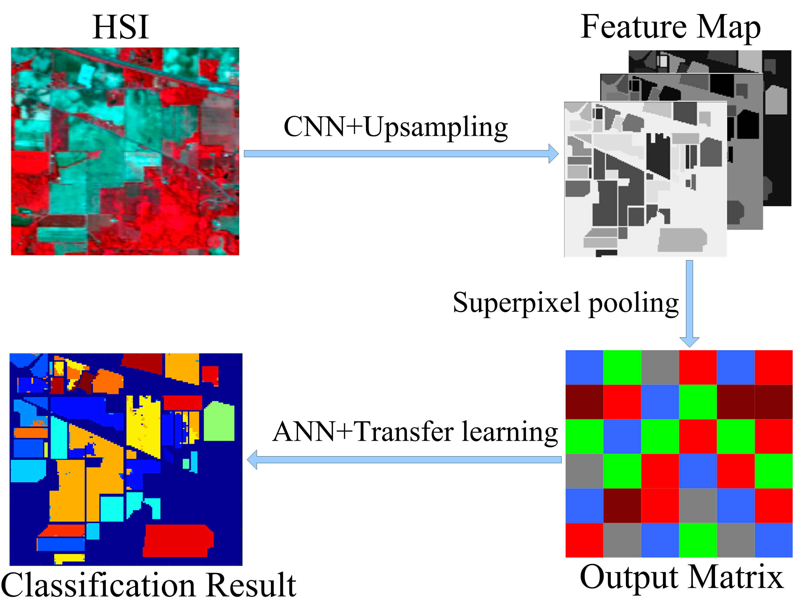
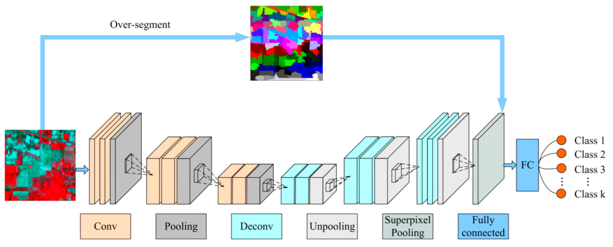
Figure 1.
The framework of the proposed superpixel pooling convolutional neural network with transfer learning (SP-CNN) method. This scheme consists of down-sampling (convolution and pooling), up-sampling (deconvolution and up-pooling), superpixel pooling and a fully connected layer.
Figure 1.
The framework of the proposed superpixel pooling convolutional neural network with transfer learning (SP-CNN) method. This scheme consists of down-sampling (convolution and pooling), up-sampling (deconvolution and up-pooling), superpixel pooling and a fully connected layer.

Figure 2.
Structure of the down-sampling in the proposed CNN model (Taking Indian Pines dataset as an example).
Figure 2.
Structure of the down-sampling in the proposed CNN model (Taking Indian Pines dataset as an example).

Figure 3.
The structure of superpixel pooling layer.

Figure 4.
Transfer learning on the SP-CNN. (a) Pre-training SP-CNN on source hyperspectral image (HSI). (b) SP-CNN classifies for target HSI.
Figure 4.
Transfer learning on the SP-CNN. (a) Pre-training SP-CNN on source hyperspectral image (HSI). (b) SP-CNN classifies for target HSI.

Figure 5.
Indian Pines image. (a) False color image. The classification maps of (b) ANN, (c) CNN, (d) CRNN, (e) CNN-PPF, (f) SS-CNN and (g) SP-CNN.
Figure 5.
Indian Pines image. (a) False color image. The classification maps of (b) ANN, (c) CNN, (d) CRNN, (e) CNN-PPF, (f) SS-CNN and (g) SP-CNN.

Figure 6.
Pavia University dataset. (a) False color image. Classification maps of (b) ANN, (c) CNN, (d) CRNN, (e) CNN-PPF, (f) SS-CNN and (g) SP-CNN.
Figure 6.
Pavia University dataset. (a) False color image. Classification maps of (b) ANN, (c) CNN, (d) CRNN, (e) CNN-PPF, (f) SS-CNN and (g) SP-CNN.

Figure 7.
Slinas dataset. (a) False color image. The classification maps of (b) ANN, (c) CNN, (d) CRNN, (e) CNN-PPF, (f) SS-CNN and (g) SP-CNN.
Figure 7.
Slinas dataset. (a) False color image. The classification maps of (b) ANN, (c) CNN, (d) CRNN, (e) CNN-PPF, (f) SS-CNN and (g) SP-CNN.

Figure 8.
Variation of classification accuracy with the increase of number of training samples.

Figure 9.
Changes of classification accuracy with the increase of the number of superpixels.


Table 1.
Parameters setting in CNN model.
| Layer | Kernelsize | Number of Kernels | Padding | Stride | Output Size |
|---|---|---|---|---|---|
| Conv_1 | 5 × 5 × 200 | 20 | 0 | 1 | 141 × 141 × 20 |
| Conv_2 | 3 × 3 × 20 | 30 | 0 | 2 | 70 × 70 × 30 |
| Max Pooling_1 | 2 × 2 | - | - | 2 | 35 × 35 × 30 |
| Conv_3 | 5 × 5 × 30 | 40 | 1 | 1 | 33 × 33 × 40 |
| Conv_4 | 3 × 3 × 40 | 60 | 0 | 2 | 16 × 16 × 60 |
| Max Pooling_2 | 2 × 2 | - | - | 2 | 8 × 8 × 60 |
| Conv_5 | 5 × 5 × 60 | 60 | 0 | 1 | 4 × 4 × 60 |
| Conv_6 | 3 × 3 × 60 | 60 | 0 | 1 | 2 × 2 × 60 |
| Max Pooling_3 | 2 × 2 | - | - | 2 | 1 × 1 × 60 |
| ReLU | 1 × 1 × 60 | ||||
| Softmax | 60 |
Table 2.
Classification accuracy (%) achieved by seven different methods on Indian Pines dataset.
| Class | Train/Test | ANN | CNN | CRNN | CNN-PPF | SS-CNN | SP-CNN |
|---|---|---|---|---|---|---|---|
| Alfalfa | 3/43 | 34.65 ± 3.32 | 97.22 ± 0.42 | 100.00 | 100.00 | 100.00 | 100.00 |
| Corn-notill | 30/1398 | 65.58 ± 5.72 | 62.02 ± 2.84 | 70.03 ± 2.86 | 67.99 ± 4.72 | 71.29 ± 1.64 | 89.62 ± 0.92 |
| Corn-mintill | 30/800 | 43.59 ± 3.73 | 87.79 ± 0.79 | 85.37 ± 2.04 | 66.46 ± 1.48 | 66.46 ± 1.48 | 98.12 ± 0.02 |
| Corn | 30/207 | 34.30 ± 2.35 | 51.98 ± 5.88 | 76.21 ± 3.92 | 79.66 ± 1.44 | 75.33 ± 1.52 | 100.00 |
| Grass-pasture | 30/453 | 81.04 ± 4.28 | 78.53 ± 0.64 | 83.07 ± 0.80 | 90.53 ± 2.24 | 93.23 ± 0.21 | 99.77 ± 0.12 |
| Grass-trees | 30/700 | 93.28 ± 2.45 | 97.22 ± 0.29 | 97.22 ± 0.20 | 95.78 ± 0.64 | 96.67 ± 0.26 | 100.00 |
| Grass-pasturemowed | 2/26 | 65.22 ± 1.49 | 100.00 | 100.00 | 98.55 ± 0.08 | 94.45 ± 0.16 | 100.00 |
| Hay-windrowed | 30/488 | 95.83 ± 0.3 | 98.16 ± 0.16 | 99.78 ± 0.08 | 99.45 ± 0.06 | 100.00 | 99.55 ± 0.04 |
| Oats | 1/19 | 36.63 ± 5.05 | 100.00 | 100.00 | 100.00 | 100.00 | 100.00 |
| Soybean-notill | 30/942 | 61.92 ± 3.13 | 78.84 ± 1.26 | 52.27 ± 1.62 | 75.49 ± 6.21 | 78.69 ± 2.82 | 88.85 ± 1.37 |
| Soybean-mintill | 30/2425 | 78.95 ± 3.32 | 61.92 ± 5.88 | 61.90 ± 4.82 | 83.64 ± 1.24 | 87.64 ± 1.64 | 89.36 ± 1.82 |
| Soybean-clean | 30/563 | 55.37 ± 7.37 | 80.31 ± 0.84 | 82.21 ± 1.04 | 76.99 ± 1.44 | 63.97 ± 3.05 | 95.38 ± 0.84 |
| Wheat | 30/175 | 93.03 ± 0.95 | 95.97 ± 0.86 | 98.97 ± 0.16 | 100.00 | 100.00 | 99.42 ± 0.26 |
| Woods | 30/1235 | 95.34 ± 2.5 | 96.59 ± 0.24 | 99.58 ± 0.01 | 99.64 ± 0.11 | 99.68 ± 0.02 | 99.43 ± 0.06 |
| Building-grass-trees | 30/356 | 42.78 ± 12.13 | 63.05 ± 4.82 | 76.32 ± 2.54 | 98.30 ± 0.72 | 97.34 ± 0.29 | 99.43 ± 0.11 |
| Stone-steel-towers | 6/87 | 86.29 ± 1.39 | 98.67 ± 0.04 | 97.61 ± 0.75 | 99.09 ± 0.06 | 98.79 ± 0.06 | 100.00 |
| OA | 66.04 ± 5.83 | 73.89 ± 1.73 | 75.92 ± 1.88 | 82.38 ± 1.26 | 83.67 ± 0.84 | 94.45 ± 0.24 | |
| AA | 60.77 ± 2.74 | 81.68 ± 1.90 | 82.75 ± 2.85 | 89.07 ± 2.07 | 88.97 ± 1.67 | 96.43 ± 0.14 | |
| Kappa | 62.75 ± 1.12 | 71.28 ± 0.93 | 72.23 ± 0.82 | 81.23 ± 0.28 | 82.7 ± 1.29 | 93.44 ± 0.20 |
Table 3.
Statistical results of six methods on Pavia University dataset.
| Class | Train/Test | ANN | CNN | CRNN | CNN-PPF | SS-CNN | SP-CNN |
|---|---|---|---|---|---|---|---|
| Asphalt | 30/6601 | 62.85 ± 12.37 | 87.26 ± 1.38 | 68.48 ± 2.32 | 86.76 ± 1.54 | 86.36 ± 2.25 | 91.13 ± 1.03 |
| Meadows | 30/18619 | 58.68 ± 2.23 | 83.53 ± 1.26 | 85.96 ± 1.63 | 81.36 ± 1.36 | 85.50 ± 1.02 | 98.72 ± 0.21 |
| Gravel | 30/2069 | 46.56 ± 9.28 | 98.20 ± 0.99 | 99.32 ± 0.08 | 99.15 ± 0.23 | 99.95 ± 0.02 | 99.67 ± 0.04 |
| Trees | 30/3034 | 53.45 ± 8.40 | 56.24 ± 1.93 | 71.63 ± 5.06 | 77.62 ± 1.17 | 79.13 ± 2.07 | 78.34 ± 3.06 |
| Metal sheets | 30/1315 | 88.82 ± 3.51 | 88.68 ± 0.72 | 94.13 ± 1.56 | 85.25 ± 1.56 | 85.13 ± 1.07 | 99.34 ± 0.06 |
| Bare soil | 30/4999 | 59.57 ± 6.12 | 95.24 ± 0.66 | 98.84 ± 0.05 | 97.02 ± 0.37 | 96.32 ± 0.17 | 97.10 ± 0.42 |
| Bitumen | 30/1300 | 88.81 ± 4.27 | 99.50 ± 0.02 | 100.0 | 100.0 | 100.0 | 100.0 |
| Bricks | 30/3652 | 76.16 ± 2.26 | 92.90 ± 0.87 | 93.68 ± 0.65 | 93.27 ± 0.52 | 94.49 ± 0.22 | 99.45 ± 0.03 |
| Shadows | 30/917 | 81.34 ± 4.02 | 79.05 ± 4.24 | 86.05 ± 1.04 | 87.31 ± 2.52 | 87.59 ± 1.42 | 88.45 ± 2.03 |
| OA | 65.78 ± 2.94 | 80.63 ± 0.75 | 82.84 ± 0.64 | 86.53 ± 0.28 | 88.02 ± 0.12 | 93.18 ± 0.12 | |
| AA | 75.59 ± 3.57 | 86.96 ± 0.31 | 88.39 ± 0.25 | 89.01 ± 0.30 | 90.15 ± 0.18 | 93.78 ± 0.25 | |
| Kappa | 57.65 ± 2.04 | 77.61 ± 0.20 | 80.84 ± 0.12 | 84.34 ± 0.26 | 85.24 ± 0.04 | 92.36 ± 0.13 |
Table 4.
Summary of classification results of six classifiers on Salinas dataset.
| Class | Train/Test | ANN | CNN | CRNN | CNN-PPF | SS-CNN | SP-CNN |
|---|---|---|---|---|---|---|---|
| Weeds_1 | 30/1979 | 100.0 | 100.0 | 100.0 | 100.0 | 100.0 | 100.0 |
| Weeds_2 | 30/3696 | 92.42 ± 0.13 | 99.27 ± 0.02 | 99.66 ± 0.04 | 99.90 ± 0.02 | 99.89 ± 0.01 | 99.89 ± 0.02 |
| Fallow | 30/1946 | 100.0 | 100.0 | 100.0 | 100.0 | 100.0 | 100.0 |
| Fallow_P | 30/1364 | 99.54 ± 0.03 | 99.29 ± 0.04 | 99.54 ± 0.07 | 99.62 ± 0.01 | 99.26 ± 0.02 | 99.89 ± 0.01 |
| Fallow_S | 30/2648 | 95.28 ± 0.53 | 98.35 ± 0.06 | 97.94 ± 1.34 | 99.38 ± 0.04 | 99.43 ± 0.08 | 98.45 ± 0.02 |
| Stubble | 30/3929 | 99.03 ± 0.38 | 99.42 ± 0.02 | 99.98 ± 0.01 | 99.97 ± 0.01 | 100.0 | 99.56 ± 0.02 |
| Celery | 30/3549 | 99.20 ± 0.12 | 99.84 ± 0.01 | 99.96 ± 0.01 | 99.92 ± 0.03 | 99.32 ± 0.04 | 99.26 ± 0.02 |
| Grapes_U | 30/11241 | 61.69 ± 2.53 | 79.30 ± 10.59 | 86.52 ± 3.11 | 86.73 ± 1.92 | 90.92 ± 1.43 | 95.63 ± 0.14 |
| Soil | 30/6173 | 97.32 ± 0.72 | 94.59 ± 1.84 | 98.40 ± 0.02 | 97.57 ± 0.05 | 99.96 ± 0.01 | 99.53 ± 0.02 |
| Corn | 30/3248 | 72.06 ± 7.72 | 73.92 ± 0.73 | 95.52 ± 0.40 | 96.12 ± 0.13 | 96.02 ± 0.20 | 99.64 ± 0.04 |
| Lettuce_4wk | 30/1038 | 91.23 ± 2.24 | 99.20 ± 0.01 | 99.20 ± 0.01 | 99.20 ± 0.21 | 99.10 ± 0.17 | 99.22 ± 0.06 |
| Lettuce_5wk | 30/1897 | 97.46 ± 0.03 | 100.0 | 100.0 | 100.0 | 100.0 | 100.0 |
| Lettuce_6wk | 30/886 | 95.24 ± 0.05 | 96.24 ± 0.04 | 96.44 ± 0.03 | 99.04 ± 0.07 | 99.28 ± 0.04 | 100.0 |
| Lettuce_7wk | 30/1040 | 91.75 ± 0.57 | 98.02 ± 0.92 | 96.38 ± 0.68 | 99.23 ± 0.63 | 100.0 | 100.0 |
| Vineyard_U | 30/7238 | 48.58 ± 5.27 | 40.81 ± 0.55 | 56.37 ± 7.88 | 71.54 ± 2.93 | 84.52 ± 1.06 | 87.36 ± 2.10 |
| Vineyard_T | 30/1777 | 91.37 ± 2.81 | 98.15 ± 0.29 | 99.03 ± 0.04 | 99.31 ± 0.12 | 99.66 ± 0.04 | 99.49 ± 0.02 |
| OA | 82.18 ± 1.92 | 88.22 ± 1.36 | 88.63 ± 0.20 | 90.24 ± 1.02 | 91.44 ± 0.19 | 95.99 ± 0.07 | |
| AA | 89.14 ± 2.28 | 90.50 ± 0.31 | 91.22 ± 0.48 | 91.36 ± 0.25 | 92.66 ± 0.05 | 95.97 ± 0.06 | |
| Kappa | 80.22 ± 1.62 | 87.88 ± 0.62 | 87.98 ± 0.05 | 89.57 ± 0.08 | 90.97 ± 0.13 | 95.46 ± 0.05 |
Table 5.
Running time (seconds) of six classification schemes on three datasets with no more than 30 labeled pixels per class.
Table 5.
Running time (seconds) of six classification schemes on three datasets with no more than 30 labeled pixels per class.
| Indian Pines | Pavia University | Salinas | ||
|---|---|---|---|---|
| ANN | Training | 3200 | 3560 | 4800 |
| Testing | 3.2 | 4.25 | 3.26 | |
| CNN | Training | 1800 | 2160 | 3600 |
| Testing | 0.21 | 0.37 | 0.26 | |
| CRNN | Training | 2900 | 2480 | 4800 |
| Testing | 1.2 | 1.7 | 1.3 | |
| CNN-PPF | Training | 21,600 | 3600 | 43,200 |
| Testing | 5 | 17 | 21 | |
| SS-CNN | Training | 1620 | 630 | 1680 |
| Testing | 0.74 | 1 | 0.78 | |
| SP-CNN | Training | 366 | 320 | 510 |
| Testing | 0.34 | 0.65 | 0.5 |
Table 6.
Overall accuracy and computational time (s) of SP-CNN for different network layers on three datasets.
Table 6.
Overall accuracy and computational time (s) of SP-CNN for different network layers on three datasets.
| SP-CNN-4 | SP-CNN-6 | SP-CNN-8 | |
|---|---|---|---|
| Parameters | ≈600,000 | ≈900,000 | ≈1,600,000 |
| Indian Pines | 92.34% | 93.46% | 93.57% |
| 290 s | 366 s | 880 s | |
| Pavia University | 92.61% | 93.18% | 93.40% |
| 280 s | 320s | 765 s | |
| Salinas | 95.51% | 95.99% | 96.12% |
| 420 s | 510 s | 930 s |
Table 7.
Effect of transfer learning on training efficiency for three datasets.
| Without Pre-Training | Indian Pines_PT | Pavia University_PT | Salinas_PT | |
|---|---|---|---|---|
| Indian Pines (>93.5%) | 366 s | / | 560 s | 768 s |
| Pavia University (>93.2%) | 760 s | 626 s | / | 320 s |
| Salinas (>95.9%) | 2060 s | 1096 s | 510 s | / |
Publisher’s Note: MDPI stays neutral with regard to jurisdictional claims in published maps and institutional affiliations. |
© 2021 by the authors. Licensee MDPI, Basel, Switzerland. This article is an open access article distributed under the terms and conditions of the Creative Commons Attribution (CC BY) license (http://creativecommons.org/licenses/by/4.0/).
Share and Cite
MDPI and ACS Style
Xie, F.; Gao, Q.; Jin, C.; Zhao, F. Hyperspectral Image Classification Based on Superpixel Pooling Convolutional Neural Network with Transfer Learning. Remote Sens. 2021, 13, 930. https://doi.org/10.3390/rs13050930
AMA Style
Xie F, Gao Q, Jin C, Zhao F. Hyperspectral Image Classification Based on Superpixel Pooling Convolutional Neural Network with Transfer Learning. Remote Sensing. 2021; 13(5):930. https://doi.org/10.3390/rs13050930
Chicago/Turabian StyleXie, Fuding, Quanshan Gao, Cui Jin, and Fengxia Zhao. 2021. "Hyperspectral Image Classification Based on Superpixel Pooling Convolutional Neural Network with Transfer Learning" Remote Sensing 13, no. 5: 930. https://doi.org/10.3390/rs13050930
Note that from the first issue of 2016, this journal uses article numbers instead of page numbers. See further details here.