Outlier Detection at the Parcel-Level in Wheat and Rapeseed Crops Using Multispectral and SAR Time Series

Abstract

This paper studies the detection of anomalous crop development at the parcel-level based on an unsupervised outlier detection technique. The experimental validation is conducted on rapeseed and wheat parcels located in Beauce (France). The proposed methodology consists of four sequential steps: (1) preprocessing of synthetic aperture radar (SAR) and multispectral images acquired using Sentinel-1 and Sentinel-2 satellites, (2) extraction of SAR and multispectral pixel-level features, (3) computation of parcel-level features using zonal statistics and (4) outlier detection. The different types of anomalies that can affect the studied crops are analyzed and described. The different factors that can influence the outlier detection results are investigated with a particular attention devoted to the synergy between Sentinel-1 and Sentinel-2 data. Overall, the best performance is obtained when using jointly a selection of Sentinel-1 and Sentinel-2 features with the isolation forest algorithm. The selected features are co-polarized (VV) and cross-polarized (VH) backscattering coefficients for Sentinel-1 and five Vegetation Indexes for Sentinel-2 (among us, the Normalized Difference Vegetation Index and two variants of the Normalized Difference Water). When using these features with an outlier ratio of 10%, the percentage of detected true positives (i.e., crop anomalies) is equal to 94.1% for rapeseed parcels and 95.5% for wheat parcels.

1. Introduction

Monitoring crop growth and status is a major challenge in remote sensing for agriculture [1]. Multispectral images have been used for this purpose for many years, thanks to their convenient interpretation and exploitation [2,3,4,5]. Synthetic aperture radar (SAR) images have also been widely studied since they are available regardless of sunlight and cloud coverage conditions [6,7,8,9,10]. The complementarity of these two types of images has been used to address problems including crop type classification [11,12], estimation of crop water requirement [13] and change detection [14,15,16]. The joint use of SAR and multispectral images is also encouraged by the large amount of free data provided by the Sentinel-1 (S1) and Sentinel-2 (S2) satellites operated by the European Space Agency (ESA). The fine spatial and temporal resolutions of S1 and S2 images allow working at the parcel-level with a high revisit frequency, which is well suited for precision agriculture [17,18]. Various studies have introduced methodologies for deriving crop classification maps using S1 and S2 data [19,20,21]. A comprehensive analysis of the temporal behavior of S1 and S2 data have also been proposed [13,22].

This work addresses an interesting remaining challenge in precision agriculture, namely the automatic detection of crop parcels that have an anomalous vegetation development. Detecting crop parcels whose phenological behaviors significantly differ from the others could help users such as farmers or agricultural cooperatives to optimize agricultural practices, disease detection or fertilization management. It could also be valuable in areas such as subsidy control or crop insurance.

In the literature, the problem of finding objects that are unusual or different from the majority of the data is known as outlier detection (also referred to as anomaly detection). Outlier detection methods have received a considerable attention [23,24,25] since they are used in a large variety of application domains, e.g., fraud detection or medical diagnosis. In the Earth observation area, various methods have been introduced to detect abnormal vegetation areas at the country-level using time series constructed from the Normalized Difference Vegetation Index (NDVI). These approaches aim at modeling NDVI time series using historical data and detecting potential anomalies by comparing new observations with their corresponding predicted values [26,27,28,29,30]. Recent studies have investigated similar techniques with S1 and S2 data, as for instance in Kanjir et al. [31] where Breaks for Additive Season and Trend (BFAST) are used to detect land use anomalies. However, these approaches can be difficult to implement for crop monitoring since modeling the normal behavior of the data implies having access to normal representative examples, which can be complex and time consuming in practice. Crop rotation, lack of historical data and the inconsistency of S2 time series due to the cloud coverage are other factors leading to a harder practical implementation (e.g., applying the BFAST algorithm to analyze a unique growing season is not adapted since this algorithm relies on a Season Trend modeling that needs multiple seasons to be calibrated). In previous work conducted in Albughdadi et al. [32], agronomic features have been extracted from multispectral images to detect outliers in crop parcels. Nevertheless, this approach was based on clustering (using the mean shift algorithm), whose parameters are not easy to adjust for the detection of abnormal crop parcels. This literature overview motivates the need to investigate new approaches for outlier detection dedicated to crop monitoring.

Rather than detecting inter-annual abnormalities, a method investigated in this paper consists in detecting the most abnormal parcels within a growing season (or a part of a growing season). In the literature, such method is referred to as point outlier detection ([24], Section 2.2). Point outlier detection consists in comparing each instance of the dataset (here, each crop parcel) to the rest of the data to find the most different instances, which are isolated from the majority of the observed data. Point outlier detection approaches are well suited to our problem since (1) they are unsupervised by nature (i.e., a training set using nominal data is not necessary), (2) they can be used with multiple indicators providing information about the crop development and (3) they can be applied to data acquired within the growing season (i.e., no historical data are needed).

This paper provides a methodology to detect anomalous crop development using SAR and multispectral images acquired by S1 and S2 sensors. The novelty of this work for crop monitoring is that it uses unsupervised outlier detection algorithms within a single growing season analysis, without any prior knowledge on the normal behavior of the parcels and using SAR and multispectral data jointly. The two main objectives of this study are: (1) to provide a detailed analysis of the different anomalies detectable with S1 and S2 data that could affect crops such as wheat and rapeseed and (2) to investigate the different factors that influence the detection results such as the feature sets.

This paper is structured as follows. Section 2 presents the study area and the data used for the detection of outlier crop parcels. Section 3 proposes the methodology suggested to detect anomalous crop development at the parcel-level. In particular, a description of the different types of agronomic outliers encountered during the study is provided. Section 4 validates the detection results for rapeseed and wheat crops. Finally, some conclusions and future work are reported in Section 5.

2. Study Area and Data

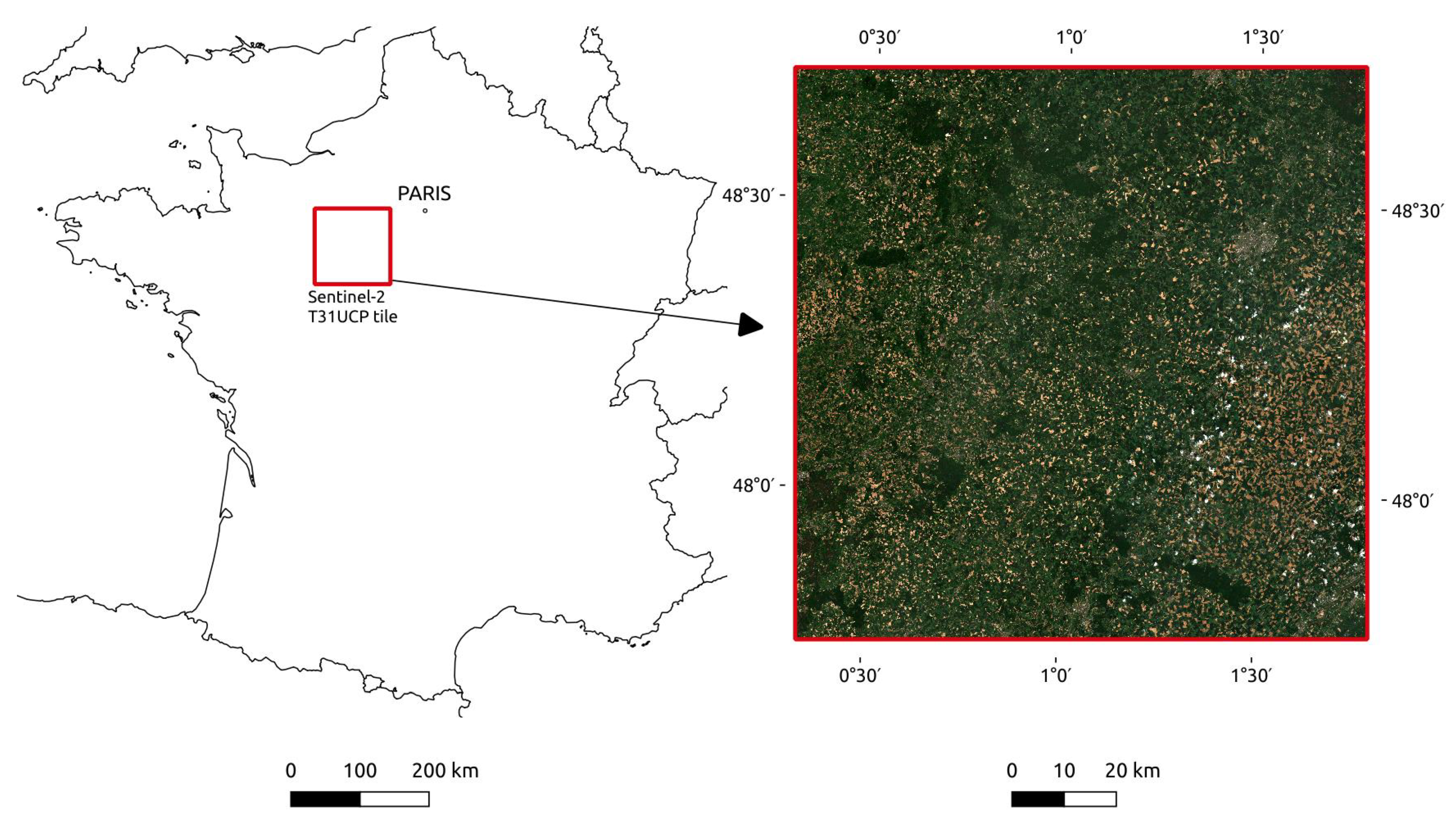
This section presents the study area and the data used for the analysis, which consist of parcel delineations and satellite data.

2.1. Study Area

The analyzed area is located in the Beauce region in France. The area has an extent of $109.8\times 109.8$ ${\mathrm{km}}^2$ and is centered approximately at 48°24${}^{\prime }$ N latitude and 1°00${}^{\prime }$ E longitude (corresponding to the T31UCP S2 tile). Figure 1 shows the tile location and the studied area, which was chosen due to its richness of large crop fields such as wheat and rapeseed.

2.2. Parcel Data

The analysis is conducted on a total of 2218 rapeseed parcels (associated with the 2017/2018 growing season) and 3361 wheat parcels (associated with the 2016/2017 growing season). To avoid problems in parcel boundaries, a buffer of 10 m was applied allowing too small parcels (area less than 0.5 ha) to be discarded from the database. In the Supplementary Materials, the robustness of the proposed method to changes in the parcel boundaries is validated using 2118 rapeseed parcel delineations resulting from the French Land Parcel Identification System (LPIS) [33], which is available in open license.

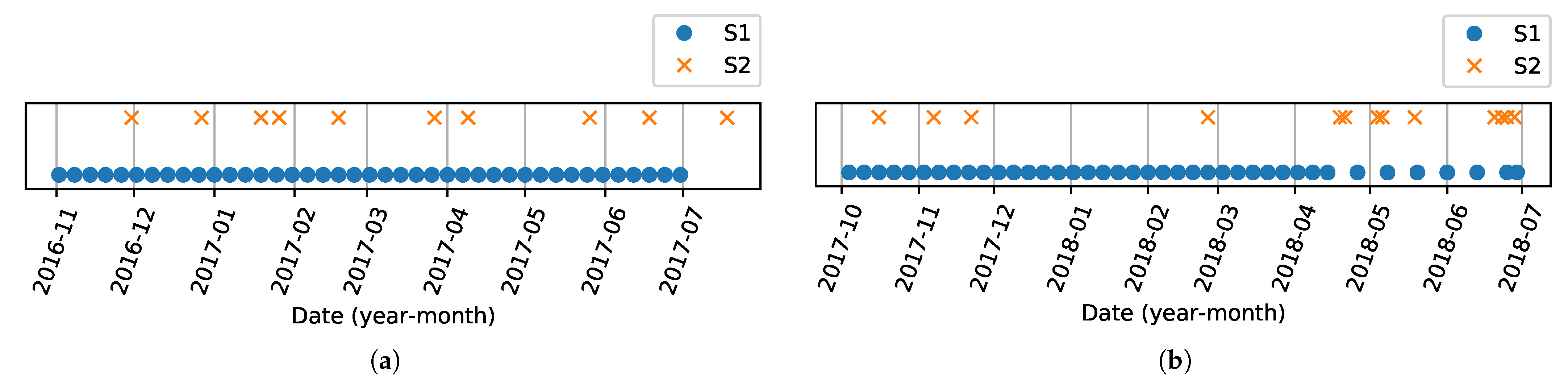
2.3. Remote Sensing Data

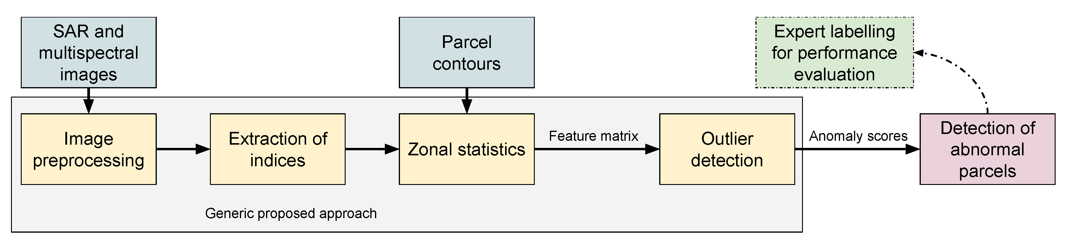
The S2 and S1 images used in this study were selected and downloaded from the PEPS platform (Plateforme d’Exploitation des Produits Sentinel) of the French National Center for Space Studies (Centre National d’Études Spatiales, CNES, https://peps.cnes.fr/, online accessed 8 December 2020). For multispectral data, both S2-A and S2-B satellites were used, which makes a theoretical revisit time of 5 days. S2 images have 13 spectral bands covering the visible, the near infra-red (NIR) and the shortwave-infrared (SWIR) spectral region [34]. Spectral bands used in the analysis to extract agronomic features at the pixel-level are reported in

Table 1. Sentinel-2 multispectral bands used for the analysis.

Spectral Bands	Central Wavelength ($\mathsf{\mu }$m)	Bandwith ($\mathsf{\mu }$m)	Resolution (m)
Band 3: Green	$0.560$	$0.035$	10
Band 4: Red	$0.665$	$0.030$	10
Band 5: Vegetation Red Edge	$0.705$	$0.015$	20
Band 8: Near Infrared (NIR)	$0.842$	$0.115$	10
Band 11: Shortwave Infrared (SWIR)	$1.610$	$0.090$	20

.

Radar S1 images are constructed by analyzing the response signal in flight direction of a C-band synthetic aperture radar (SAR) operating at a center frequency of 5.405 GHz. Both S1-A and S1-B satellites were used in ascending orbit (6 days revisit time). Ground Range Detected (GRD) products were used in the Interferometric Wide (IW) swath mode: phase information is lost but the volume of data is considerably reduced. All SAR images were available in dual polarization (VH+VV) with a 10 m spatial resolution [35].

The acquisition dates of S1 and S2 images are depicted in Figure 2 for the 2016/2017 and 2017/2018 growing seasons. One interest of analyzing two different growing seasons is to evaluate the robustness of the proposed method to changes in the satellite data. It was decided to select S2 images with a low cloud coverage (cloud coverage lower than 20%). The strategy considered to handle remaining clouds is detailed in Section 3.1. All S1 images covering the analyzed area in ascending orbit were selected. For the 2016/2017 growing season, 41 S1 images and 10 S2 images were selected whereas 40 S1 images and 13 S2 images were selected in 2017/2018. Due to cloud coverage, the acquisition dates for S2 images are very different for the two growing seasons. Note that a reduced number of S1 images were available between May and July 2018. The absence of data during this period can be observed in all web pages providing S1 data, which confirms problems in data acquisition. This absence of images is interesting since it allows the robustness of the method to missing data to be appreciated.

3. Methods

The proposed method for detecting abnormal crop development relies on a four-step sequential procedure depicted in Figure 3 and discussed in detail in what follows. Methods to describe and evaluate the detection results are also provided in this section.

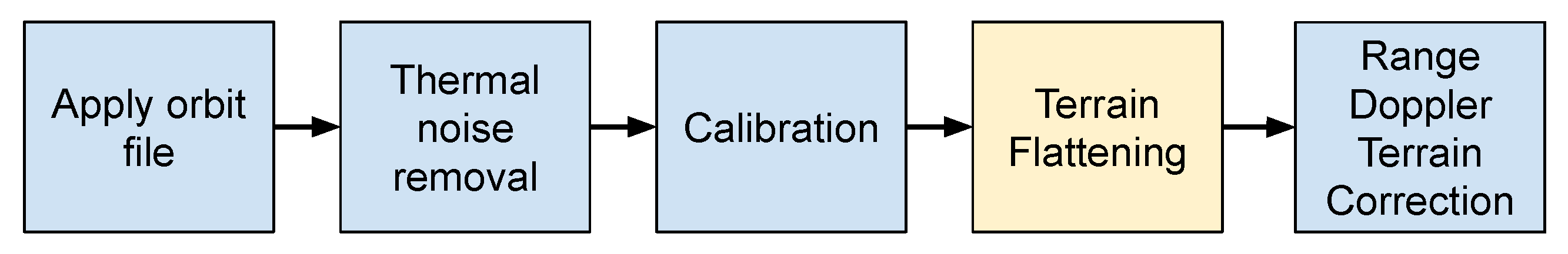
3.1. Image Preprocessing

S2 images were preprocessed using the online MAJA processing chain [36] available on the PEPS platform of CNES. This preprocessing step provides level-2A ortho-rectified products expressed in surface reflectance. In addition to atmospheric correction, level-2A images are available with a cloud and shadow mask discarding irrelevant pixels in the images. A resampling strategy was adopted to obtain a spatial resolution of 10 m for the channels with a lower spatial resolution. Parcels fully covered by clouds during at least one time instant were discarded from the database and parcels partially covered by clouds were analyzed using pixels not covered by the cloud mask (the shadow mask was used in a similar way).

To build the database of S1 images, an offline processing (illustrated in Figure 4) was conducted with the Sentinel Application Platform (SNAP, version 7.0, http://step.esa.int/main/toolboxes/snap/, online accessed 8 December 2020). This processing is inspired by the workflow proposed in Filipponi [37]. A Terrain-Flattening operation was added to take into account the local incidence angles, as the analyzed area is wide and parcel features are compared to each other. This operation uses the Shuttle Radar Topography Mission (SRTM) Digital Elevation Model (DEM). The Range Doppler terrain correction provides orthorectified images. Note that a multi-temporal speckle filtering step was also tested without significant differences on the results (we implemented our own Python version of the filter introduced in Equation (14) of Quegan and Jiong Jiong Yu [38]). The best results were obtained with the workflow of Figure 4 (Supplementary Figure S15).

3.2. Extraction of SAR and Multispectral Features at the Pixel-Level

The following section describes the pixel-level features derived from multispectral and SAR images considered in this work (reported in

Table 2. Pixel-level features computed from S2 and S1 images used in this paper. For S2, The near infrared (band 8), red edge (band 5), short wave infrared (band 11), green (band 3) and red (band 4) channels are denoted as NIR, RE, SWIR, GREEN and RED, respectively.

Sensor Type	Indicator	Formula
Multispectral	NDVI	$\left(\mathrm{NIR}-\mathrm{RED}\right)/\left(\mathrm{NIR}+\mathrm{RED}\right)$
	${\mathrm{NDWI}}_{\mathrm{SWIR}}$	$\left(\mathrm{NIR}-\mathrm{SWIR}\right)/\left(\mathrm{NIR}+\mathrm{SWIR}\right)$
	${\mathrm{NDWI}}_{\mathrm{GREEN}}$	$\left(\mathrm{GREEN}-\mathrm{NIR}\right)/\left(\mathrm{GREEN}+\mathrm{NIR}\right)$
	$\mathrm{MCARI}/\mathrm{OSAVI}$	$\left((\mathrm{RE}-\mathrm{IR})-0.2\times (\mathrm{RE}-\mathrm{RED})\right)/\left((1+0.16)\times \frac{\mathrm{NIR}-\mathrm{RED}}{\mathrm{NIR}+\mathrm{RED}+0.16}\right)$
	GRVI	$\left(\mathrm{GREEN}-\mathrm{RED}\right)/\left(\mathrm{GREEN}+\mathrm{RED}\right)$
SAR	Cross-polarized backscattering coefficient VH	${\gamma }_{\mathrm{VH}}^0$
	Co-polarized backscattering coefficient VV	${\gamma }_{\mathrm{VV}}^0$

) and their importance for monitoring crop growth. It was observed that choosing irrelevant features can lead to poor detection results, since unsupervised algorithms use all the features available for the analysis. For post-analysis and practical applications, it is also important to choose features whose interpretation is convenient in order to understand why an anomaly has been detected.

3.2.1. Multispectral Vegetation Indices

Many multispectral Vegetation Indices (VIs) have been introduced in the literature e.g., [2,39]. A VI relates the acquired spectral information to the observed vegetation, and thus allows better quantitative and qualitative evaluations of the vegetation covers. The five multispectral VIs considered in this paper are reported in Table 2 and described below. Note that raw S2 bands were also tested without any improvement in the detection precision and a more difficult interpretation of the results when compared to VIs.

The NDVI is a benchmark indicator for agronomic analyses and is mainly related to the plant vigor [2,40]. The Normal Difference Water Index (NDWI) actually refers to two different widely used indicators. The first version uses Near infrared (NIR) and Short Wave infrared (SWIR) to monitor changes in the water content of leaves [41]. The second version uses the green band and NIR to monitor changes related to content in water bodies [42]. Both formulas are similar to NDVI with different bands involved. The SWIR version of NDWI seems to be more appropriate for crop analysis but the GREEN version of NDWI can also provide relevant information, e.g., for flooded parcels. The Modified Chlorophyll Absorption Ratio Index (MCARI) was designed to extract information from the chlorophyll content in plants with a resistance to the variation of the Leaf Area Index (LAI). A variant called MCARI/OSAVI uses the Optimized Soil Adjusted Vegetation Index (OSAVI) to minimize the contribution of background reflectance [39,43]. The Green Red Vegetation Index (GRVI) is similar to NDVI but uses the red and green bands. According to [44], GRVI “can be a site-independent single threshold for detection of the early phase of leaf green-up and the middle phase of autumn coloring” (referred to as senescence for crops).

3.2.2. SAR Features

Many investigations have been performed to establish a relationship between SAR images and vegetation and have been reported in two recent reviews [9,10]. The backscattering coefficients (denoted as ${\gamma }_{\mathrm{VH}}^0$ and ${\gamma }_{\mathrm{VV}}^0$) have been used intensively in the literature [7,45]. The polarization ratio ${\gamma }_{\mathrm{VH}}^0/{\gamma }_{\mathrm{VV}}^0$, also used in various studies [18,19,22,46] was tested without showing any clear improvement. The same observation stands for the Radar Vegetation Index (RVI) [8], which has been adapted to S1 with an alternative form $4{\sigma }_{\mathrm{VH}}^0/({\sigma }_{\mathrm{VH}}^0+{\sigma }_{\mathrm{VV}}^0)$ [47]. Thus, the results presented in this paper have been obtained with the backscattering coefficients reported in Table 2.

3.3. Input Data for the Outlier Detection Algorithms

This section explains the steps needed to have parcel-level features, which will be used as inputs for the outlier detection algorithm.

3.3.1. Extraction of Parcel-Level Features with Zonal Statistics

The pixel-level features are averaged through spatial statistics referred to as “zonal statistics” in order to provide parcel-level features. Two zonal statistics are considered for the S2 VIs, namely the median and interquartile range (IQR). The median captures the mean behavior of a given parcel with more robustness than the classical mean as it is not affected by extreme values [48]. It is used to detect anomalies affecting the entire crop parcel, such as anomalies in crop vigor. IQR is defined as the difference between the 75th and 25th percentiles. It contains information related to the heterogeneity of a given parcel while being robust to the presence of extreme values. These statistics were computed using the Python libraries SciPy version 1.4.1 [49] and rasterstats version 0.13.0 (https://pythonhosted.org/rasterstats/, online accessed 8 December 2020). Since cloud and shadow pixels were discarded, these statistics were computed from the remaining pixels after applying the cloud and shadow masks. Other zonal statistics were also tested, namely the skewness (which is related to the asymmetry of a distribution) and the kurtosis (which can be used to characterize the tail of a distribution) but led to a deterioration of the detection results (Supplementary Figure S14). The SAR feature set was reduced to the median of the backscatter intensities, as IQR of S1 data was found to be directly proportional to the median.

3.3.2. Feature Matrix

Each parcel is represented by a vector concatenating the zonal statistics computed for all pixel-level features at each date. The construction of the feature matrix, used as the input of the outlier detection algorithms, is illustrated in

Table 3. Simplified version of the feature matrix using NDVI only and two statistics (median/IQR) for n dates and M parcels. NDVI${}_{t_n}$ means NDVI computed for image $\#n$ and median${}_{P_M}$ means spatial median of the feature computed inside the parcel $\#M$.

Parcel #	Feature 1	Feature 2	.	Feature L-1	Feature L
$P_1$	median${}_{P_1}$(NDVI${}_{t_0}$)	IQR${}_{P_1}$(NDVI${}_{t_0}$)	.	median${}_{P_1}$(NDVI${}_{t_n}$)	IQR${}_{P_1}$(NDVI${}_{t_n}$)
$P_2$	median${}_{P_2}$(NDVI${}_{t_0}$)	IQR${}_{P_2}$(NDVI${}_{t_0}$)	.	median${}_{P_2}$(NDVI${}_{t_n}$)	IQR${}_{P_2}$(NDVI${}_{t_n}$)
...	...	...	.	...	...
$P_M$	median${}_{P_M}$(NDVI${}_{t_0}$)	IQR${}_{P_M}$(NDVI${}_{t_0}$)	.	median${}_{P_M}$(NDVI${}_{t_n}$)	IQR${}_{P_M}$(NDVI${}_{t_n}$)

when using the NDVI with 2 statistics. In the general case, the number of columns of this matrix is $N_{col}=N_{1,im}\times N_{1,f}\times N_{1,s}+N_{2,im}\times N_{2,f}\times N_{2,s}$, where $N_{1,im}$ is the number of S1 images, $N_{1,f}$ is the number of pixel-level features extracted for each S1 image, $N_{1,s}$ is the number of statistics computed for each S1 feature and similar definitions apply to $N_{2,im}$, $N_{2,f}$ and $N_{2,s}$ for S2 images. As each column corresponds to a unique combination statistics/feature/time, it is possible to compare each parcel column-wise. Note that classical preprocessings such as the Principal Component Analysis (PCA) [50] or the Multidimensional Scaling (MDS) [51] were applied to this feature matrix without significant improvement regarding the outlier detection results. Thus, these preprocessing were ignored from our analysis.

3.4. Outlier Detection Algorithms

Using the feature matrix whose construction is detailed in the previous section, an outlier detection algorithm attributes to each parcel an outlier score. The percentage of the most abnormal parcels to be detected is called the outlier ratio (i.e., the parcels that have the highest outlier score).

The experiments presented in this document were conducted using the Isolation Forest (IF) algorithm [52], which provided the best results overall. IF is an isolation-based technique that assumes that anomalies can be easily isolated in “a tree structure based on random cuts in the values of randomly selected features in the dataset” [53]. IF is considerably fast since it does not need computation of distances or density measures. The number of isolation trees was fixed to ${\mathrm{n}}_{\mathrm{trees}}=1000$ and the size of the data sub-sampling was fixed to ${\mathrm{n}}_{\mathrm{samples}}=256$, as in the original paper. Changing these two parameters did not have a significant effect on the results, which is a crucial advantage compared to the other algorithms (see Section 4.3 for more details).

Three other outlier detection algorithms were also tested, namely: One-Class Support Vector Machine (OC-SVM) [54], Local Outlier Probabilities (LoOP) [55], and AutoEncoder (AE) ([23], Section 3.6). These algorithms are based on different ideas, making them interesting for comparison purposes. The effect of changing the algorithm used for the detection is discussed in Section 4.3 and details regarding the choice of the hyperparameters are provided in the Supplementary Materials. To run the experiments conducted in this study, the Python Scikit-learn (version 0.23.0) implementations of OC-SVM and IF were used [56]. The Python library PyNomaly (version 0.3.3) was used for the implementation of the LoOP algorithm [57]. Finally, we implemented our own autoencoder with the Python library Keras (https://keras.io/, online accessed 8 December 2020) (version 2.3.0).

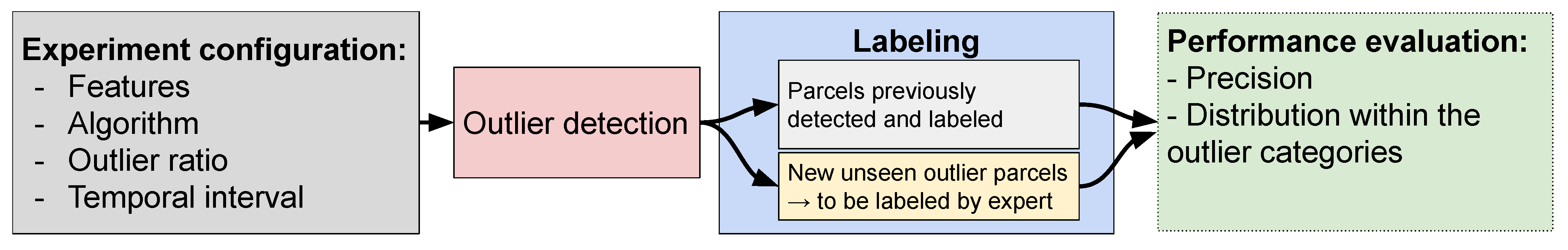
3.5. Experiments Conducted to Evaluate the Proposed Method

In what follows, what is called “experiment” corresponds to an outlier detection conducted with a specific initial configuration (set of features, algorithm, outlier ratio, temporal interval) using one of the two datasets (wheat or rapeseed). Various experiments were conducted to evaluate the proposed approach: each time a new set of features or a new algorithm tuning was tested, the parcels declared as outliers were counterchecked by experts (if not previously detected), confirming the anomaly (true positive) or not (false positive), and determining the type of anomaly (see details later). This iterative procedure is illustrated in Figure 5.

For the rapeseed dataset, 252 initial configurations were tested to evaluate the factors that can influence the detection results. Most of these experiments were conducted on a complete growing season to evaluate the capacity of the proposed approach to detect anomalies occurring at different periods of the crop growth, and to determine whether differences between the detected parcels can be observed or not. Some other experiments were also made with a lower amount of data, in particular for a mid-season analysis between October and February. Early detection can be of interest for warning purposes at the beginning of the growth cycle and gives more details on the effect of having only few data available for the analysis. The influence of the amount of parcels to be detected (called outlier ratio) is also tested to analyze the relevance of the outlier score given to each parcel.

For the wheat dataset, 25 experiments were made: the main idea was to determine whether our approach can be applied with minor modifications to other kinds of crops. The different experiments conducted during the study are reported in

Table 4. Summary of the evaluated factors analyzed throughout the study. In parenthesis, the number of different initial configurations tested (features, algorithm, time interval, outlier ratio).

Evaluated Crop Type	Time Interval	Evaluated Factors
Rapeseed (252)	Complete season (218)	Outlier detection algorithms
		Feature sets
		Outlier ratio
		Zonal statistics
		Missing S2 images
		Changes in parcel boundaries
	Mid-season (34)	Feature sets, algorithms, outlier ratio
Wheat (25)	Complete season (20)	Feature sets, algorithm
	Mid-season (5)	Feature sets, algorithm

. The main results obtained from a selection of these experiments are presented in this document whereas additional results are discussed in Section 4.3.

3.6. Description of the Outlier Parcels

The outlier parcels were identified through multiple outlier detection analyses presented in Section 3.5. With the help of agronomic experts, the labeling of the detected parcels was conducted by visual-interpretation using all the available S1 and S2 images and by using all the time series of the different features/statistics to compare any analyzed parcel to the rest of the dataset. Each labeled parcel was assigned to one of the outlier categories described in what follows.

3.6.1. Outlier Categories

The different anomalies analyzed throughout the study can be decomposed into 4 main categories: heterogeneity problems, growth anomalies, database errors and others. The category “others” corresponds to non-agronomic outliers that were considered not relevant for crop monitoring (referred to as false positives). A brief description of each category is proposed in

Table 5. Description of the different categories of anomalies detected during the labeling process. Subcategories were added to have a more precise description. For each category TP means true positive, considered relevant for crop monitoring, and FP means false positive, considered irrelevant for crop monitoring.

Category (TP/FP)	Subcategory	Description
Heterogeneity (TP)	Heterogeneity	Affects the parcel most of the season
	Heterogeneity (2 different parts)	The parcel is separated into two homogeneous different parts
	Heterogeneity after senescence	Occurs during senescence phase
	Early heterogeneity	Occurs during early growing season
Growth (TP)	Late growth	A late development is observed (non-vigorous crop)
	Vigorous crop	A vigorous development is observed
	Early flowers	Early flowering phase
	Early senescence	Early senescence phase
	Late senescence	Late senescence phase
Error in database (TP)	Wrong type	A wrong crop type is reported in the database
	Wrong shape	The parcel boundaries are not accurately reported
Others (FP)	Normal (counterchecked)	The parcel was declared normal by the agronomic expert
	Too small	The parcel is too small, causing abnormal features
	SAR anomaly	Soil surface conditions cause abnormal SAR features
	Shadow perturbation (cloud or forest)	Shadows cause abnormality in the features.

and more details and examples are provided below. Additional examples are also available in the Supplementary Materials.

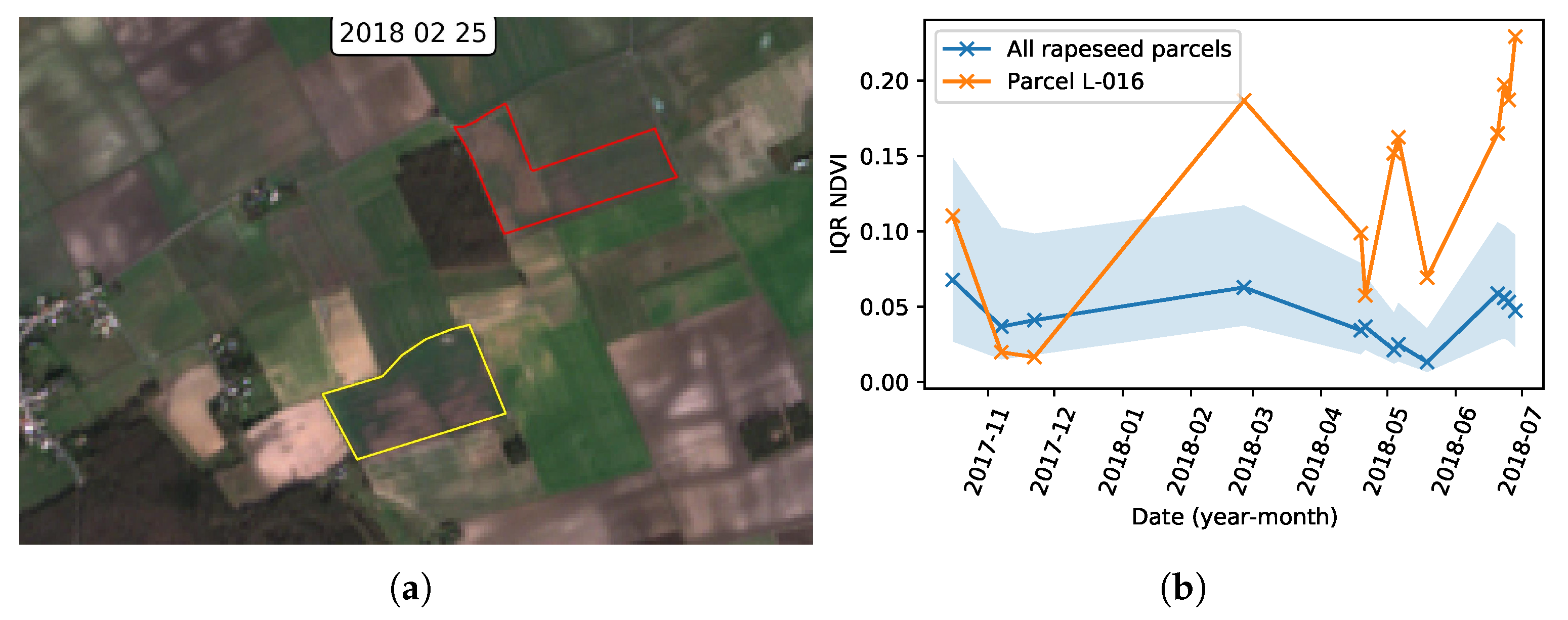
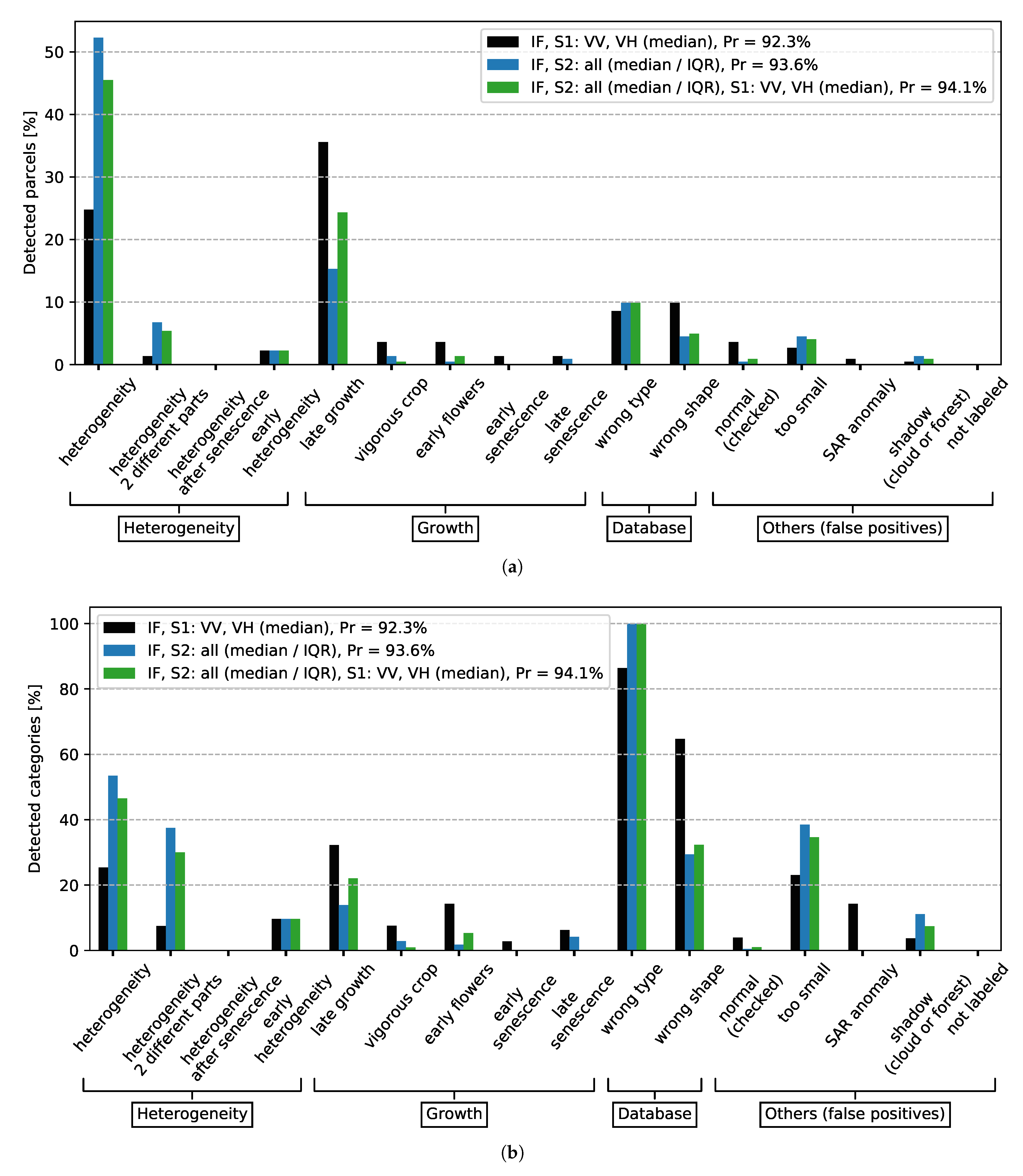
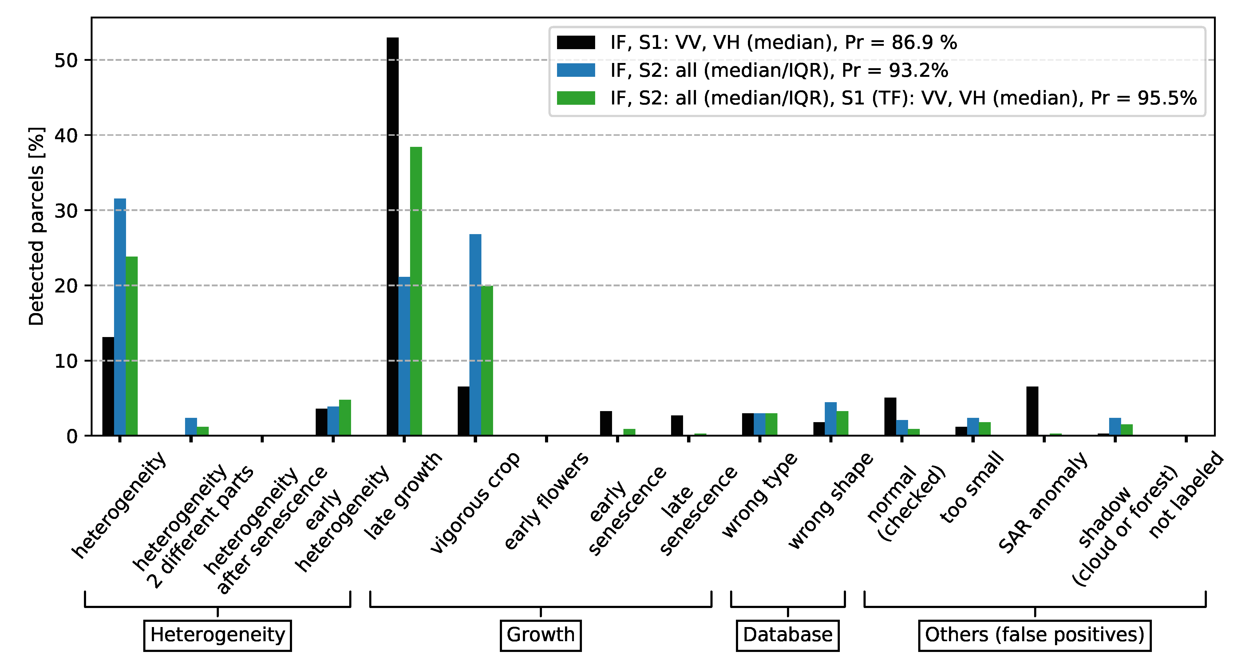
• Heterogeneity corresponds to parcels presenting a clear heterogeneous development (i.e., spatially heterogeneous development). The most common cases of heterogeneity can be observed all along the growing season and are for instance related to soil heterogeneity, presence of weed or diseases. An example of heterogeneous parcel is shown in Figure 6. More transient cases of heterogeneity can affect the beginning (early heterogeneity) or the end of the growing season (heterogeneity after senescence) and can be for instance related to differences in soil characteristics or parcel exposure (Supplementary Figure S2). Heterogeneity (2 different parts) parcels have two areas of the same crop separated by a clear frontier (e.g., strong difference in the phenological stages) (Supplementary Figure S1).
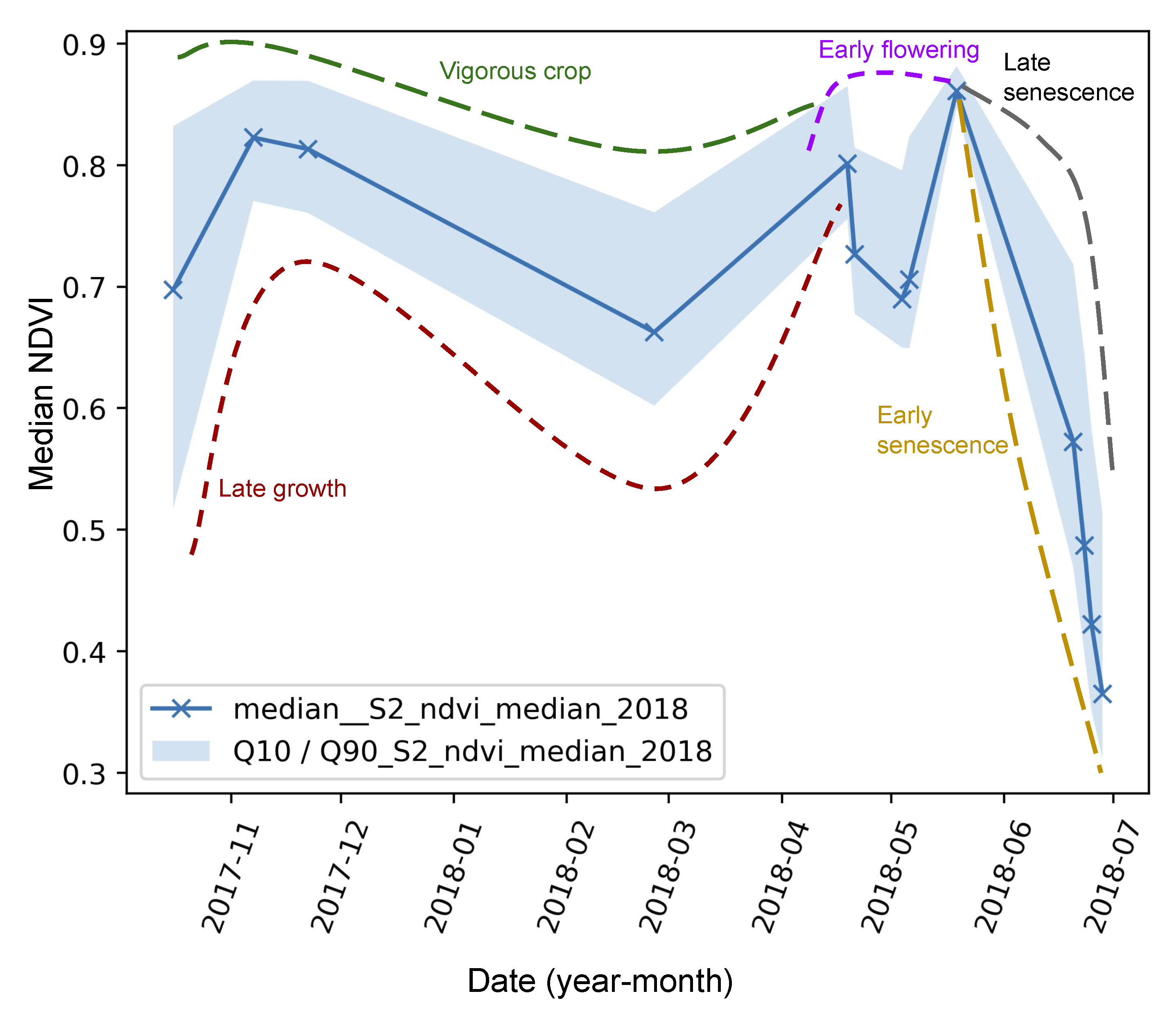
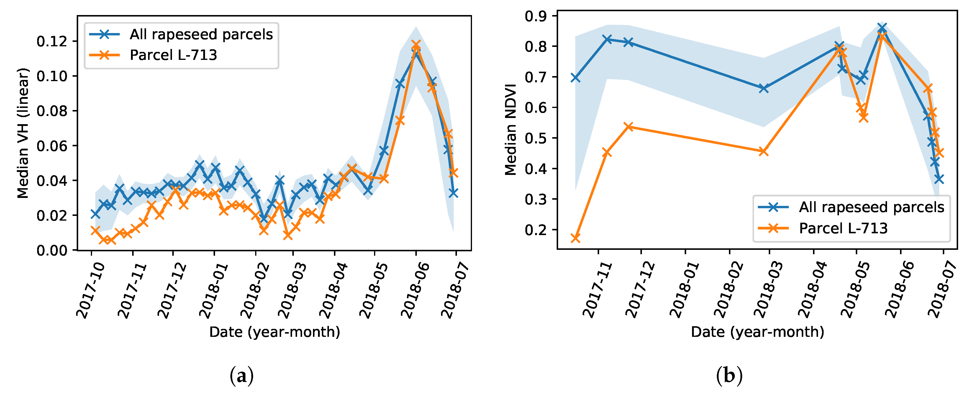
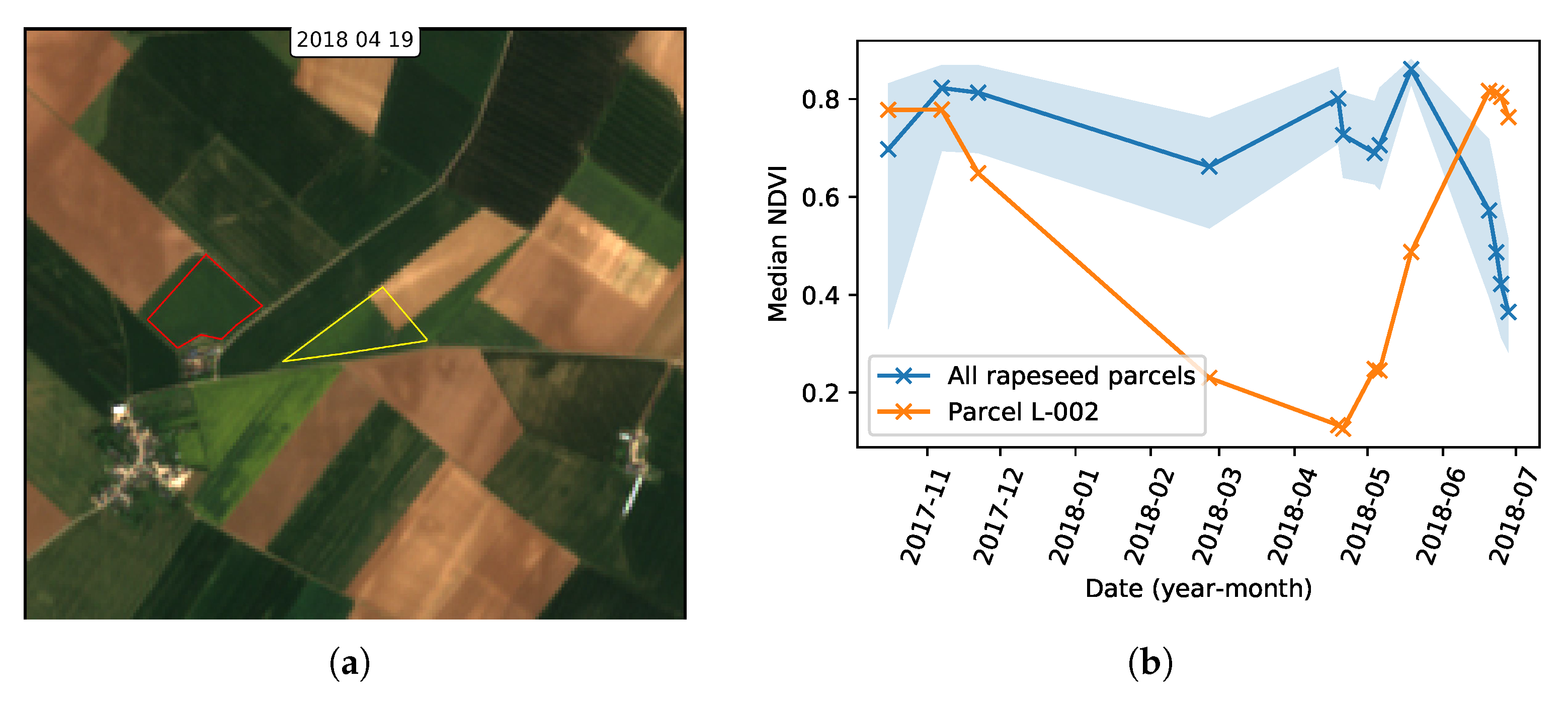
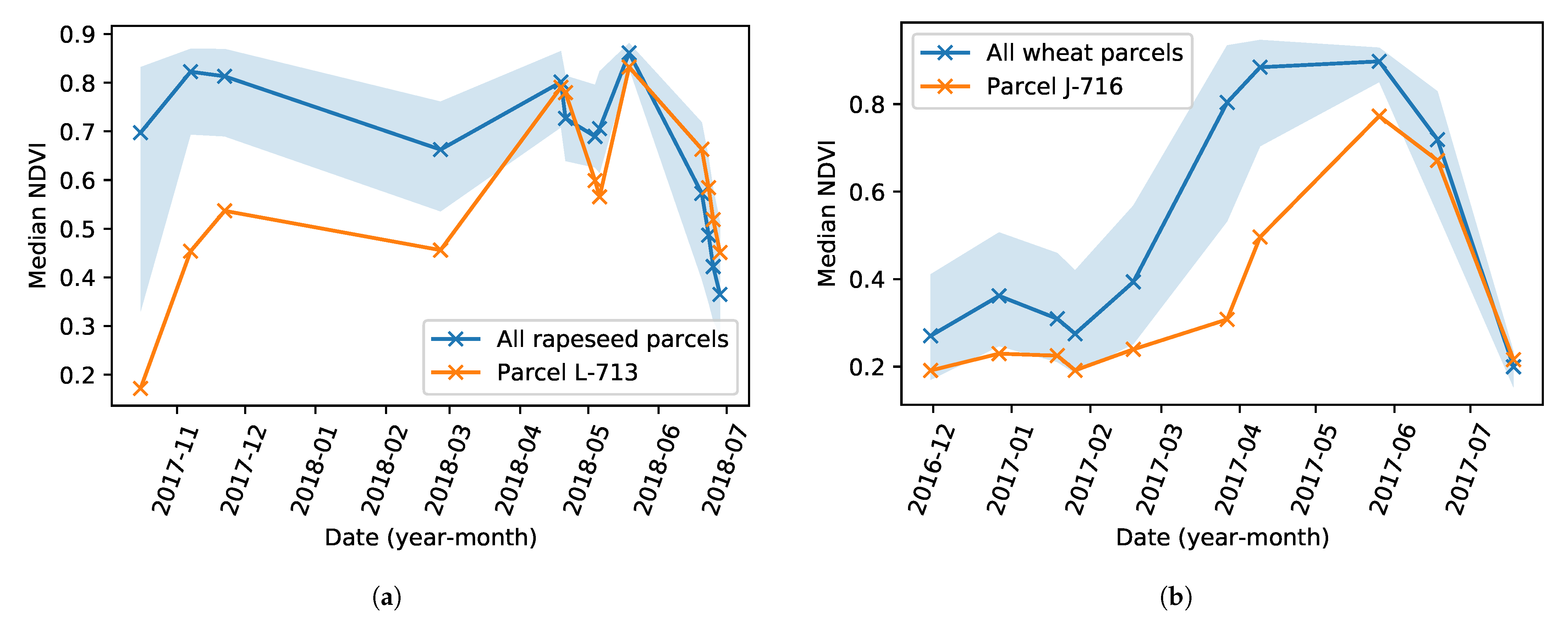
• Growth anomalies are related to an abnormal development of the crop. The two main categories of growth anomalies are parcels with a low vigor (late growth) or, on the contrary, with a high vigor (vigorous crop). Figure 7 illustrates how the different growth anomalies can affect the median NDVI of the parcels within a growing season. Figure 8 provides an example of growth anomaly where the S1 VH time series is affected by a late growth issue. As for heterogeneity, more transient growth anomalies, such as a delay in the flowering or senescence phase, can affect a crop parcel (Supplementary Figure S5).
• Database errors are considered as relevant anomalies to be detected. This type of error is a common problem in large databases and can be challenging and time consuming to be detected manually. Examples of “wrong shape” and “wrong type” parcels reported in the database are provided in Figure 9. This category of anomalies presents in general a strong sign of abnormality. Note that a “wrong shape” parcel can be caused by a farmer using part of a neighborhood parcel or by an inaccurate delineation reported in the database. Note also that a “wrong type” parcel can be confirmed using another database such as the French LPIS.
• The “Normal (checked)” label was given to parcels that were labeled as normal after inspecting the features and images. In some cases, some few extreme values were observed explaining why the parcel was detected as abnormal by the outlier detection algorithms. In any case, all these parcels should have an outlier score (i.e., the score given by an outlier detection algorithm) lower than the parcels affected by agronomic anomalies (e.g., heterogeneity or growth anomaly).
• Other non-agronomic anomalies considered as false positives concern a few percentage of the analyzed parcels. Some very small parcels were still present in the dataset and are labeled as “too small” (it is sometimes difficult to clean efficiently too small parcels that are long and narrow). Analyzing this type of parcels is not possible due to the spatial resolution of Sentinel data. These parcels were kept in the database to illustrate problems that can occur in practical applications. “Shadow” is another kind of non-agronomic anomaly that can be caused by forests near the parcel (Supplementary Figure S6) or clouds that are not detected using the cloud mask.
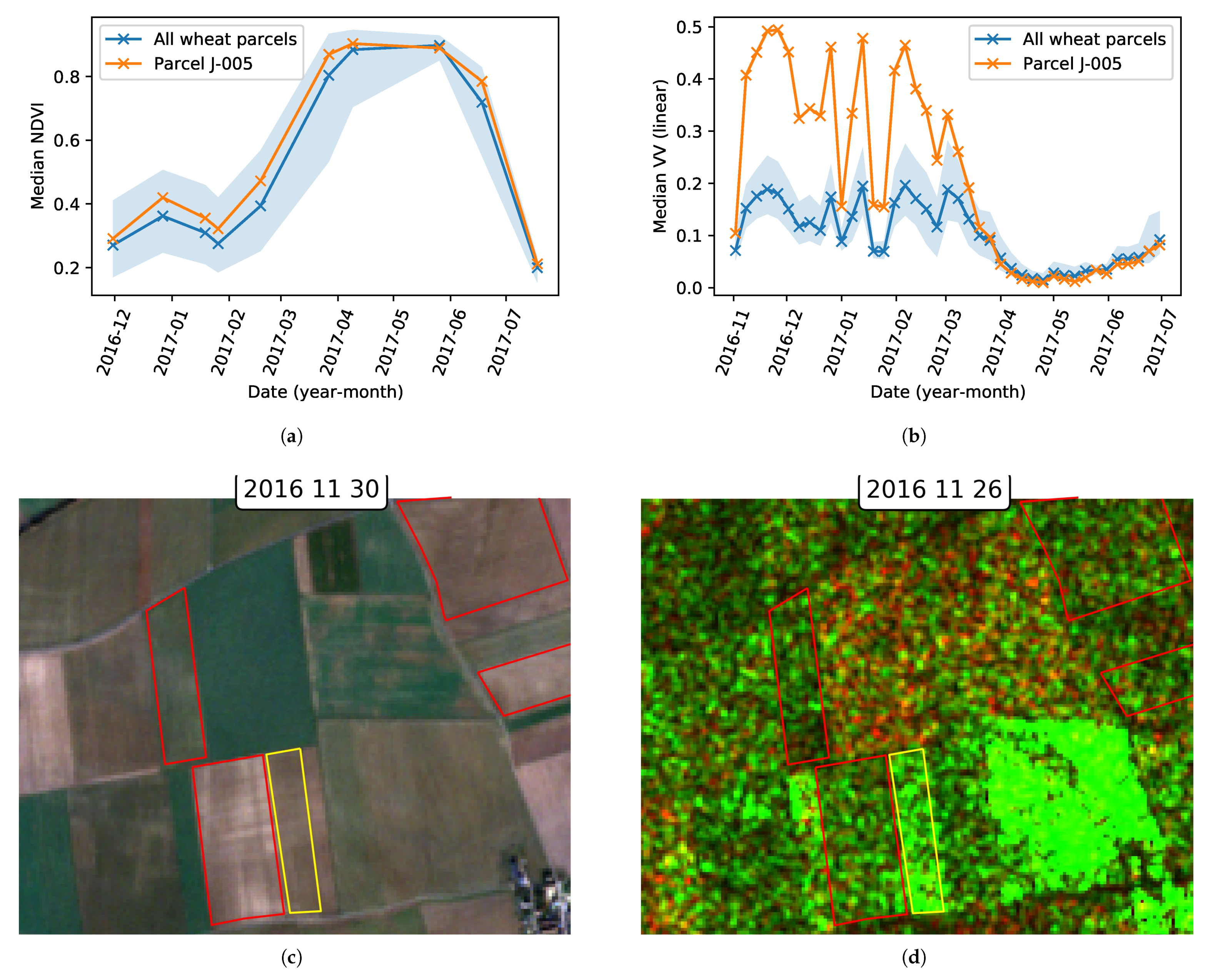
• A subcategory of non-agronomic anomalies are “SAR anomalies”. These anomalies correspond to parcels where SAR features have an abnormal time evolution in early growing season (i.e., the SAR indicators are abnormal compared to the rest of the data), whereas multispectral images and their features were counterchecked as normal. It is a known issue in crop monitoring with SAR data that was studied in Wegmuller et al. [58], Wegmüller et al. [59], Marzahn et al. [60], which is reported as a “Flashing field” phenomenon. These anomalies are considered as non-agronomic since SAR data are affected by other factors than the vegetation status such as soil moisture, soil structure, row orientation or soil roughness. This kind of anomalies was observed more frequently for wheat crops and in early growing season when there is a low vegetation cover. The “flashing field” terminology can be understood by looking at the example displayed in Figure 10.

3.6.2. Distribution of the Outlier Parcels in the Two Datasets

Figure 11 summarizes the distribution of the anomaly categories for both wheat and rapeseed crops. Approximately 55% of the rapeseed dataset was checked by the agronomic experts, ensuring that the outlier parcels analyzed in the study are representative. Similarly, 30% of the most abnormal wheat parcels were checked to validate the relevance of our method when applied to another crop type. Figure 11 shows that heterogeneity and growth problems are the most detected anomalies for both crop types.

3.7. Performance Evaluation

The precision is used to evaluate the quality of a detection and is defined as

$$\mathrm{precision}=\frac{\mathrm{TP}}{\mathrm{TP}+\mathrm{FP}}$$

(1)

where TP and FP are the numbers of true positives and false positives, respectively. The precision expresses the percentage of detected parcels that are true positives (here, agronomic anomalies checked by the experts). Plotting precision vs. outlier ratio curves is a good way to compare various detection results: for a given outlier ratio, a good algorithm or feature choice has generally detection results with a higher precision. Note that these curves also provide information regarding the false negatives samples since for a given outlier ratio, a higher precision means less false negatives. These curves are similar to the Receiver Operating Characteristics (ROC) or the precision vs. recall curves but with the advantage of being more adapted to outlier detection. Indeed, the outlier ratio can be adjusted without ground-truth, by selecting the parcels with the highest outlier scores. Moreover, when analyzing these curves one can focus on realistic values of the outlier ratio (e.g., precision obtained when detecting more than 50% of the data instances seems not adapted to our problem). The area under the precision vs. outlier ratio curve (AUC) can be used to provide a quantitative measure of detection performance summarizing the information contained in the whole curve. In the analysis, we computed the AUC for outlier ratios in the range [0, 0.5]. The AUC was then divided by 0.5 to normalize the obtained value: the resulting score can be seen as the average precision for outlier ratios in the range [0, 0.5]. Note that this representation does not give information regarding the distribution of the different detected categories since two algorithms can have the same precision without detecting the same parcels (e.g, one algorithm can detect more heterogeneous parcels whereas another one detects more late growth anomalies). Using the distribution of the different types of anomalies detected for a given outlier ratio is a complementary way to address this limitation. Note that to highlight the distribution of the false negative instances, it is possible to display the number of detected parcels in each category divided by the total number of parcels in each category.

4. Results and Discussion

The different feature combinations tested in this section are identified in the figures using abbreviations that are defined in

Table 6. Abbreviations used with their corresponding sets of features used for outlier detection. Each abbreviation can be read as follows: “S2: pixel-level features (parcel-level statistics), S1: pixel-level features (parcel-level statistics)”.

Abbreviated Name	Features Used
S1: VV, VH (median)	Median of S1 features listed in Section 3.2
S2: all (median/IQR)	Median and IQR of all S2 features listed in Section 3.2
S2: all (median/IQR), S1: VV, VH (median)	Median and IQR of all the S2 features and median of the 2 S1 features VV and VH.

.

4.1. Anomaly Detection Results for Rapeseed Crops

The results presented in this section were conducted by analyzing the complete rapeseed dataset with the IF algorithm. First, the outlier detection is conducted using only S1 features, since SAR data are available permanently through all the crop cycle, which is important for crop monitoring applications. Then, the effect of using only S2 features is investigated. Finally, S1 and S2 features are used jointly to study the effect of combining the contribution of both types of sensors.

4.1.1. Outlier Detection with S1 Features

The strength of S1 data for crop anomaly detection is confirmed when analyzing Figure 12 (black curve): the precision is equal to 92.3% for an outlier ratio fixed to 10%. For lower outlier ratios, the precision obtained when using S1 features is slightly higher than the precision obtained when using S2 features (which will be discussed later). For higher outlier ratios, the precision decreases (more false positives are detected) but remains close to 85% for an outlier ratio equal to 20%. These results highlight the ability of the IF algorithm to provide relevant outlier scores: the parcels with the highest outlier scores are more likely to be true positives. Figure 13a shows the distribution of the detected parcels in the different anomaly categories. The majority of the detected parcels are affected by late growth (35%) and heterogeneity (25%). Anomalies coming from an error in the database (wrong shape and wrong crop type reported) are also largely detected (18.5%). To further investigate these results, Figure 13b depicts for each category the percentage of detected parcels. All parcels of the category wrong type are detected, which can be understood since this anomaly strongly affects the features at a parcel-level. Using S1 features leads to detect more parcels of the category wrong shape when compared to using S2 features. A similar observation can be done for vigorous crops and early flowering to a lesser extent (for this outlier ratio, only few of these transient anomalies are detected).

4.1.2. Outlier Detection with S2 Features

Although S2 time series have lower temporal resolution when compared to S1 time series, they are useful for outlier analysis as shown in Figure 12 (blue curve). For an outlier ratio fixed to 20%, the precision of the detection obtained using only S2 features is still above 90%. Moreover, the average precision for outlier ratios in the range [0, 0.5] is equal to 87% whereas it is 80% when using S1 features only. For a complete growing season, having 13 S2 images is sufficient to detect a majority of relevant anomalies. However, S1 and S2 features tend to detect different types of anomalies as highlighted in Figure 13a. When using S2 features, the IF algorithm detects a majority of heterogeneous parcels (52%) and less late growth parcels (15%). This observation justifies the joint use of S1 and S2 features, which is investigated below. Figure 13b shows that 40% of the parcels affected by two parts heterogeneity are detected when using S2 features (only 10% are detected when using S1 features). Moreover, a larger amount of too small parcels are detected when using S2 features (around 40% whereas it is close to 20% when using S1 features). This last observation should be put in perspective with the small amount of parcels belonging to this category (less than 5% of the detected parcels).

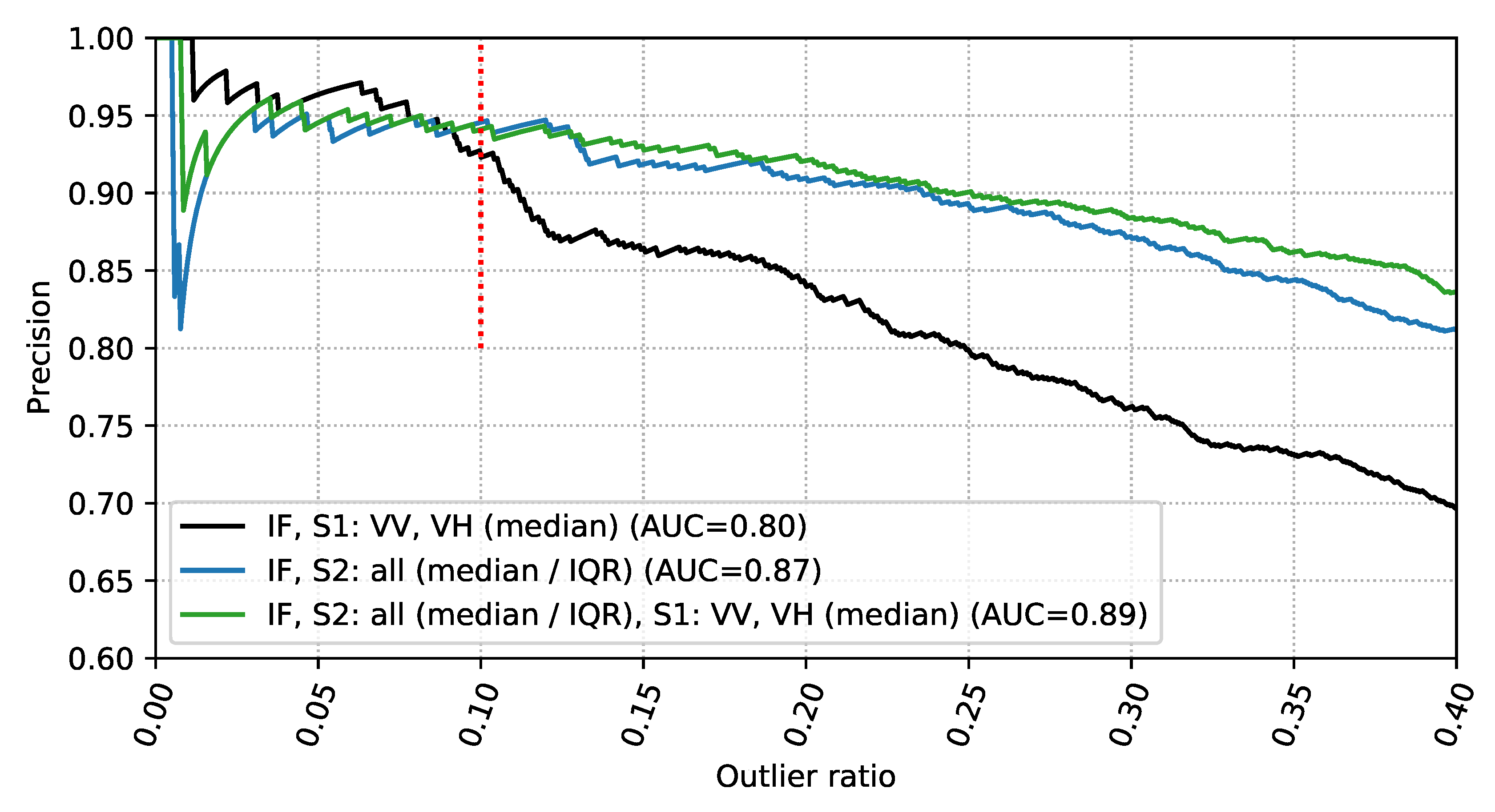
4.1.3. Outlier Detection with S1 and S2 Features

One of the main objectives of this study is to investigate the joint use of S1 and S2 for outlier detection in agricultural crops. Figure 12 (green curve) shows that the average precision obtained when using S1 and S2 features jointly is close to 89%, which is the best performance obtained for a complete growing season analysis of the rapeseed parcels. This result means that a larger amount of relevant anomalies are detected for a given outlier ratio when compared to using S1 or S2 features separately. Moreover, it also means that the IF algorithm is able to use efficiently the characteristics of each sensor. Figure 13a shows that using S1 and S2 features jointly allows the contribution of each sensor to be accounted. In particular, late growth anomalies are more detected when compared to using only S2 features (24% vs. 15% of the detected parcels) and heterogeneous parcels are more detected when compared to using only S1 features (45% vs. 25% of the detected parcels). These observations are confirmed by Figure 13b.

Overall, the best combination of features obtained throughout the study consists in using S1 and S2 features jointly. This combination exploits the strength of each sensor for crop monitoring. To be more specific, on the one hand some heterogeneous parcels are not impacting the features extracted from S1 images since this sensor is not sensitive to the color of the crop parcels. On the other hand, some anomalies affecting the crop growth are impacting more clearly the S1 time series that are more sensitive to the vegetation structure. Moreover, since S1 time series are dense, it is in some cases easier to detect late growth or senescence problems (e.g., as mentioned for the wheat crop analysis, only few S2 images were available during the senescence phase). These results are confirmed in what follows when analyzing a different crop type.

4.2. Extension to Wheat Crops

A complementary analysis was conducted to measure the robustness of the proposed method to a change in the crop type. An experiment is presented with the selection of the best features used for rapeseed crops analysis, i.e., all the features listed in Table 6. The IF algorithm was used to detect abnormal wheat parcels for a complete growing season with an outlier ratio of 10%. The distribution of the detected anomalies in the different categories is depicted in Figure 14, which also indicates the precision obtained for each detection. Again, combining S1 and S2 data leads to the best precision (95.5%). Similar to rapeseed crops, using S1 data allows more growth anomalies to be detected when compared to S2 data. The precision obtained using S1 features is lower due to a higher number of SAR anomalies (i.e., 22 SAR anomalies) but the results are still accurate (precision = 86.9%). As for the rapeseed analysis, no SAR anomaly is detected when using S1 and S2 data jointly. Finally, since less S2 images were available during the senescence phase, using S1 features logically leads to better detect problems affecting this growing phase and confirms the interest of using both types of features. These results confirm the interest of the proposed approach and its robustness to changes in the crop type.

Some differences were observed after analyzing the results obtained for rapeseed and wheat crops. These differences are interesting to analyze since they provide specific information for the monitoring of each crop type. For the wheat crops, the percentage of detected heterogeneous parcels is lower: when using S2 features, 31% of the detected wheat parcels belong to this category whereas 52% of heterogeneous parcels are detected for the rapeseed crops. On the other hand, the amount of detected vigorous parcels is higher (28% when using only S2 features) whereas few vigorous parcels were detected during the rapeseed analysis. It is also interesting to note that these parcels are more easily detected using S2 features whereas late growth anomalies are still detected in higher proportion (52%) when using S1 features.

The fact that more late growth anomalies have been detected for wheat parcels is coherent with the observations made during the labeling, where it was noticed that late growth problems frequently have a bigger impact on the wheat parcels. A representative example is provided in Figure 15: the rapeseed parcel affected by a late growth anomaly has a normal vigor after the flowering phase, whereas the wheat parcel has a low vigor for the complete growing season. It was also observed that few abnormally vigorous parcels have been detected among the rapeseed dataset: this could be related to an early sowing date and a high vigor shortly after the plant emergence as pointed out in Veloso et al. [22]. Finally, the fact that few abnormally vigorous wheat parcels have been detected when using only S1 features is also coherent with the observations made in Veloso et al. [22], where it was highlighted that the SAR signal remains stable during early growing season whereas the NDVI starts increasing after the emergence of the plant.

4.3. Influence of Other Factors on the Detection Results

Various other factors that can influence the detection results were analyzed in complement of the experiments presented in this document. A summary of the influence of each factor is available at the end of this section in

Table 7. Summary of the influence of the different analyzed factors for the detection of anomalous crop development.

Evaluated Factor	Effect and Recommendation
Outlier detection algorithm	Similar results obtained with various algorithms. IF is recommended for its robustness and easy tuning.
Outlier score	Strongest anomalies have a higher outlier score than transient anomalies, which is interesting for crop monitoring.
Missing S2 data	The proposed method is robust to missing S2 data. Using S1 dense time series improves the results.
Mid growing season analysis	Results with high precision are obtained, early analysis is possible.
Changes in parcel delineation	Small changes in the parcel delineation do not affect the detection results

.

Regarding the outlier detection algorithms, different methods for detecting anomalies lead to similar results for a complete growing season analysis (Supplementary Figures S9 and S10). However, we think that the IF algorithm is better suited for two main reasons: (1) it provides a higher precision overall during the various experiments, showing its robustness to different changes in the initial configuration, (2) the fact that no tuning is necessary is of crucial importance since the detection results are relevant without a preliminary analysis of the data. This does not hold true for autoencoders, whose hyperparameters are challenging to tune and strongly impact the detection results. For OC-SCM and LoOP, poor results were observed in the case of a mid growing season analysis, showing a lack of robustness of these methods when changing the amount of data used for the analysis.

Experiments were conducted by changing the outlier ratio and analyzing their distribution among the different categories of outliers (Supplementary Figure S13). For a low outlier ratio (e.g., 10%), the detected parcels are affected by strong agronomic anomalies (e.g., global heterogeneity, globally low vigor). It is of crucial importance because it means that the IF algorithm attributes to these parcels the highest anomaly scores, which is relevant from an agronomic point of view. Then, parcels with lower outlier scores are affected by more transient anomalies, such as senescence problems. Using an outlier ratio equal to 20% ensures the detection of the most important anomalies among the crop parcels, with a low amount of false positives when using both S1 and S2 features.

The robustness of our method was also tested regarding the impact of missing S2 images. A good precision was obtained even with a low amount of S2 images: by using half of the S2 images, a similar precision is obtained thanks to the complementary of S1 data, which is permanently available (Supplementary Figures S16 and S17). Moreover, an outlier analysis conducted on a mid growing season (all images acquired before February) was investigated in more detail. The main reasons were to (1) measure the impact of a reduced temporal interval for the analysis and (2) investigate the interest of such analysis for early warning purposes. The results (Supplementary Figures S18 and S19) show that a large number of abnormal parcels are detected with high precision and that the presented method can be used for an early growing season analysis.

Finally parcel delineations coming from the French Land Parcel Identification System (LPIS) were investigated to confirm the robustness of the proposed method to small changes in the parcel boundaries for the rapeseed parcels (Supplementary Figures S20 and S21). Our results confirm that the proposed method provides consistent results even when using parcel boundaries of lower precision.

5. Conclusions

This paper studied a new anomaly detection method for crop monitoring based on outlier analysis at the parcel-level using Sentinel-1 and Sentinel-2 features. This method is decomposed into 4 main steps: (1) preprocessing of multispectral and synthetic aperture radar (SAR) images, (2) computation of pixel-level features, (3) computation of zonal statistics at the parcel-level for all pixel-level features at each date, (4) detection of abnormal crop parcels using the isolation forest algorithm with the multi-temporal zonal statistics. The proposed method is fully unsupervised and can be used without historical data. It can be applied to different kinds of crops (such as rapeseed or wheat considered in this paper) and is able to detect a majority of parcels that are abnormal in an agronomic sense. Moreover, a relevant anomaly score is attributed to each parcel: agronomic anomalies affecting most of the growing season have a higher score than transient anomalies.

This study showed that S1 and S2 features are complementary for the detection of abnormal parcels in agricultural crops. Regarding S1 features, it is recommended using median statistics computed at the parcel-level from VV and VH backscattering coefficients. For S2 features, median and IQR statistics computed at the parcel-level from the Normalized Difference Vegetation Index (NDVI), the Green-Red Vegetation Index (GRVI), two variants of the Normalized Difference Water Index (NDWI) and a variant of the Modified Chlorophyll Absorption Ratio Index (MCARI/OSAVI) provided the best results, especially when combined with S1 features. Finally, the Isolation Forest algorithm is the outlier detection algorithm that provided the best results for identifying abnormal agricultural parcels with a simple parameter tuning.

Further investigation should be conducted to determine whether other multispectral features, e.g., biophysical parameters such as the Leaf Area Index (LAI) or the fraction of green vegetation cover (fCover) [61,62], can improve crop monitoring. Regarding SAR features, the use of SLC images could also be investigated to extract polarimetric parameters such as entropy or volume scattering and in particular the new Dual polarimetric radar vegetation index (DpRVI) considered in Mandal et al. [63]. Another line of research is to take into account the temporal structure of vegetation indices to potentially improve detection of agronomic anomalies and estimate the dates where the detected anomalies have appeared. For instance, contextual outlier detection might be interesting for disturbance or inter-annual anomaly detection. Including a contextual outlier detection in the strategy might provide complementary information to detect both inter-annual and intra-annual anomalies. Coupling the detection method with a supervised or unsupervised classification algorithm is another prospect, in order to assign to each detection an anomaly type that could be helpful for example to identify heterogeneity or growth problems automatically. It could also be interesting to investigate other types of crops such as soybean (a low biomass crop contrary to wheat and rapeseed that are both considered as high biomass crops). Finally, crop anomaly detection has several potential applications in precision agriculture at different scales. For the farmer, a weekly access to a list of parcels with abnormal behavior would help them to optimize their practices (e.g., regarding optimization of fertilization or better in-situ monitoring). For regional actors such as agricultural cooperatives or consultants, the detection of outlier parcels is useful to focus their visits on specific parcels having potential problems. Deploying and operating the proposed processing chain under operational conditions is a current challenge requiring adapted tools (e.g., for storage or processing). Finally, making the outputs of the proposed anomaly detection algorithm understandable and accessible to end-users (e.g., to farmers or companies) is an important issue to be solved using adapted web and mobile interfaces.

References

1. Weiss, M.; Jacob, F.; Duveiller, G. Remote sensing for agricultural applications: A meta-review. Remote Sens. Environ. 2020, 236, 111402. [Google Scholar] [CrossRef]
2. Bannari, A.; Morin, D.; Bonn, F.; Huete, A.R. A review of vegetation indices. Remote Sens. Rev. 1995, 13, 95–120. [Google Scholar] [CrossRef]
3. Gómez, C.; White, J.C.; Wulder, M.A. Optical remotely sensed time series data for land cover classification: A review. ISPRS J. Photogramm. Remote Sens. 2016, 116, 55–72. [Google Scholar] [CrossRef] [Green Version]
4. Inglada, J.; Vincent, A.; Arias, M.; Tardy, B.; Morin, D.; Rodes, I. Operational High Resolution Land Cover Map Production at the Country Scale Using Satellite Image Time Series. Remote Sens. 2017, 9, 95. [Google Scholar] [CrossRef] [Green Version]
5. Verrelst, J.; Camps-Valls, G.; Muñoz-Marí, J.; Rivera, J.P.; Veroustraete, F.; Clevers, J.G.; Moreno, J. Optical remote sensing and the retrieval of terrestrial vegetation bio-geophysical properties—A review. ISPRS J. Photogramm. Remote Sens. 2015, 108, 273–290. [Google Scholar] [CrossRef]
6. Betbeder, J.; Rémy, F.; Philippets, Y.; Ferro-Famil, L.; Baup, F. Contribution of multitemporal polarimetric synthetic aperture radar data for monitoring winter wheat and rapeseed crops. J. Appl. Remote Sens. 2016, 10, 026020. [Google Scholar] [CrossRef]
7. Khabbazan, S.; Vermunt, P.; Steele-Dunne, S.; Ratering Arntz, L.; Marinetti, C.; van der Valk, D.; Iannini, L.; Molijn, R.; Westerdijk, K.; van der Sande, C. Crop monitoring using Sentinel-1 Data: A Case Study from the Netherlands. Remote Sens. 2019, 11, 1887. [Google Scholar] [CrossRef] [Green Version]
8. Kumar, D.; Rao, S.; Sharma, J. Radar Vegetation Index as an Alternative to NDVI for Monitoring of Soyabean and Cotton. In Proceedings of the XXXIII INCA International Congress (Indian Cartographer), Jodhpur, India, 19–21 September 2013; Volume 33, pp. 91–96. [Google Scholar]
9. Liu, C.; Chen, Z.; Shao, Y.; Chen, J.; Hasi, T.; Pan, H. Research advances of SAR remote sensing for agriculture applications: A review. J. Integr. Agric. 2019, 18, 506–525. [Google Scholar] [CrossRef] [Green Version]
10. McNairn, H.; Shang, J. A Review of Multitemporal Synthetic Aperture Radar (SAR) for Crop Monitoring. In Multitemporal Remote Sensing: Methods and Applications; Ban, Y., Ed.; Springer International Publishing: Cham, Switzerland, 2016; Chapter 15; pp. 317–340. [Google Scholar] [CrossRef]
11. Inglada, J.; Vincent, A.; Arias, M.; Marais-Sicre, C. Improved Early Crop Type Identification By Joint Use of High Temporal Resolution SAR Furthermore, Optical Image Time Series. Remote Sens. 2016, 8, 362. [Google Scholar] [CrossRef] [Green Version]
12. Orynbaikyzy, A.; Gessner, U.; Conrad, C. Crop type classification using a combination of optical and radar remote sensing data: A review. Int. J. Remote Sens. 2019, 40, 6553–6595. [Google Scholar] [CrossRef]
13. Navarro, A.; Rolim, J.; Miguel, I.; Catalão, J.; Silva, J.; Painho, M.; Vekerdy, Z. Crop Monitoring Based on SPOT-5 Take-5 and Sentinel-1A Data for the Estimation of Crop Water Requirements. Remote Sens. 2016, 8, 525. [Google Scholar] [CrossRef] [Green Version]
14. Prendes, J.; Chabert, M.; Pascal, F.; Giros, A.; Tourneret, J.Y. Change detection for optical and radar images using a Bayesian nonparametric model coupled with a Markov random field. In Proceedings of the 2015 IEEE International Conference on Acoustics, Speech and Signal Processing (ICASSP), South Brisbane, QLD, Australia, 9–24 April 2015; pp. 1513–1517. [Google Scholar]
15. Prendes, J.; Chabert, M.; Pascal, F.; Giros, A.; Tourneret, J.Y. A new multivariate statistical model for change detection in images acquired by homogeneous and heterogeneous sensors. IEEE Trans. Image Process. 2015, 24, 799–812. [Google Scholar] [CrossRef] [PubMed] [Green Version]
16. Prendes, J.; Chabert, M.; Pascal, F.; Giros, A.; Tourneret, J.Y. Performance assessment of a recent change detection method for homogeneous and heterogeneous images. Rev. Française Photogrammétrie Télédétection 2015, 209, 23–29. [Google Scholar]
17. Defourny, P.; Bontemps, S.; Bellemans, N.; Cara, C.; Dedieu, G.; Guzzonato, E.; Hagolle, O.; Inglada, J.; Nicola, L.; Rabaute, T.; et al. Near real-time agriculture monitoring at national scale at parcel resolution: Performance assessment of the Sen2-Agri automated system in various cropping systems around the world. Remote Sens. Environ. 2019, 221, 551–568. [Google Scholar] [CrossRef]
18. Vreugdenhil, M.; Wagner, W.; Bauer-Marschallinger, B.; Pfeil, I.; Teubner, I.; Rüdiger, C.; Strauss, P. Sensitivity of Sentinel-1 backscatter to vegetation dynamics: An Austrian case study. Remote Sens. 2018, 10, 1396. [Google Scholar] [CrossRef] [Green Version]
19. Denize, J.; Hubert-Moy, L.; Betbeder, J.; Corgne, S.; Baudry, J.; Pottier, E. Evaluation of using Sentinel-1 and Sentinel-2 Time-Series to Identify Winter Land Use in Agricultural Landscapes. Remote Sens. 2018, 11, 37. [Google Scholar] [CrossRef] [Green Version]
20. Kussul, N.; Mykola, L.; Shelestov, A.; Skakun, S. Crop inventory at regional scale in Ukraine: Developing in season and end of season crop maps with multi-temporal optical and SAR satellite imagery. Eur. J. Remote Sens. 2018, 51, 627–636. [Google Scholar] [CrossRef] [Green Version]
21. Hedayati, P.; Bargiel, D. Fusion of Sentinel-1 and Sentinel-2 Images for Classification of Agricultural Areas Using a Novel Classification Approach. In Proceedings of the IGARSS 2018—2018 IEEE International Geoscience and Remote Sensing Symposium, Valencia, Spain, 22–27 July 2018; pp. 6643–6646. [Google Scholar] [CrossRef]
22. Veloso, A.; Mermoz, S.; Bouvet, A.; Toan, T.L.; Planells, M.; Dejoux, J.F.; Ceschia, E. Understanding the temporal behavior of crops using Sentinel-1 and Sentinel-2-like data for agricultural applications. Remote Sens. Environ. 2017, 199, 415–426. [Google Scholar] [CrossRef]
23. Aggarwal, C.C. Outlier Analysis, 2nd ed.; Springer International Publishing: Cham, Switzerland, 2017. [Google Scholar] [CrossRef]
24. Chandola, V.; Banerjee, A.; Kumar, V. Survey of Anomaly Detection. ACM Comput. Surv. 2009, 41, 15:1–15:58. [Google Scholar] [CrossRef]
25. Pimentel, M.; Clifton, D.; Clifton, L.; Tarassenko, L. A Review of Novelty Detection. Signal Process. 2014, 99, 215–249. [Google Scholar]
26. Atzberger, C.; Eilers, P.H.C. Evaluating the effectiveness of smoothing algorithms in the absence of ground reference measurements. Int. J. Remote Sens. 2011, 32, 3689–3709. [Google Scholar] [CrossRef]
27. Beck, P.S.; Atzberger, C.; Høgda, K.A.; Johansen, B.; Skidmore, A.K. Improved monitoring of vegetation dynamics at very high latitudes: A new method using MODIS NDVI. Remote Sens. Environ. 2006, 100, 321–334. [Google Scholar] [CrossRef]
28. Klisch, A.; Atzberger, C. Operational Drought Monitoring in Kenya Using MODIS NDVI Time Series. Remote Sens. 2016, 8, 267. [Google Scholar] [CrossRef] [Green Version]
29. Meroni, M.; Fasbender, D.; Rembold, F.; Atzberger, C.; Klisch, A. Near real-time vegetation anomaly detection with MODIS NDVI: Timeliness vs. accuracy and effect of anomaly computation options. Remote Sens. Environ. 2019, 221, 508–521. [Google Scholar] [CrossRef]
30. Verbesselt, J.; Zeileis, A.; Herold, M. Near real-time disturbance detection using satellite image time series. Remote Sens. Environ. 2012, 123, 98–108. [Google Scholar] [CrossRef]
31. Kanjir, U.; Đurić, N.; Veljanovski, T. Sentinel-2 Based Temporal Detection of Agricultural Land Use Anomalies in Support of Common Agricultural Policy Monitoring. ISPRS Int. J. Geo-Inf. 2018, 7, 405. [Google Scholar] [CrossRef] [Green Version]
32. Albughdadi, M.; Kouamé, D.; Rieu, G.; Tourneret, J.Y. Missing data reconstruction and anomaly detection in crop development using agronomic indicators derived from multispectral satellite images. In Proceedings of the 017 IEEE International Geoscience and Remote Sensing Symposium (IGARSS), Fort Worth, TX, USA, 23–28 July 2017; pp. 5081–5084. [Google Scholar] [CrossRef]
33. Barbottin, A.; Bouty, C.; Martin, P. Using the French LPIS database to highlight farm area dynamics: The case study of the Niort Plain. Land Use Policy 2018, 73, 281–289. [Google Scholar] [CrossRef]
34. Drusch, M.; Del Bello, U.; Carlier, S.; Colin, O.; Fernandez, V.; Gascon, F.; Hoersch, B.; Isola, C.; Laberinti, P.; Martimort, P.; et al. Sentinel-2: ESA’s Optical High-Resolution Mission for GMES Operational Services. Remote Sens. Environ. 2012, 120, 25–36. [Google Scholar] [CrossRef]
35. Torres, R.; Snoeij, P.; Geudtner, D.; Bibby, D.; Davidson, M.; Attema, E.; Potin, P.; Rommen, B.; Floury, N.; Brown, M.; et al. GMES Sentinel-1 mission. Remote Sens. Environ. 2012, 120, 9–24. [Google Scholar] [CrossRef]
36. Hagolle, O.; Huc, M.; Villa Pascual, D.; Dedieu, G. A multi-temporal and multi-spectral method to estimate aerosol optical thickness over land, for the atmospheric correction of FormoSat-2, LandSat, VENμS and Sentinel-2 images. Remote Sens. 2015, 7, 2668–2691. [Google Scholar] [CrossRef] [Green Version]
37. Filipponi, F. Sentinel-1 GRD Preprocessing Workflow. In Proceedings of the 3rd International Electronic Conference on Remote Sensing, 22 May–5 June 2019; Volume 18, p. 11. [Google Scholar] [CrossRef] [Green Version]
38. Quegan, S.; Yu, J.J. Filtering of multichannel SAR images. IEEE Trans. Geosci. Remote Sens. 2001, 39, 2373–2379. [Google Scholar] [CrossRef]
39. Wu, C.; Niu, Z.; Tang, Q.; Huang, W. Estimating chlorophyll content from hyperspectral vegetation indices: Modeling and validation. Agric. For. Meteorol. 2008, 148, 1230–1241. [Google Scholar] [CrossRef]
40. Rouse, J.; Haas, R.; Schell, J.; Deering, D. Monitoring vegetation systems in the Great Plains with ERTS. NASA Spec. Publ. 1974, 351, 309. [Google Scholar]
41. Gao, B. NDWI—A normalized difference water index for remote sensing of vegetation liquid water from space. Remote Sens. Environ. 1996, 58, 257–266. [Google Scholar] [CrossRef]
42. McFeeters, S.K. The use of the Normalized Difference Water Index (NDWI) in the delineation of open water features. Int. J. Remote Sens. 1996, 17, 1425–1432. [Google Scholar] [CrossRef]
43. Daughtry, C.; Walthall, C.; Kim, M.; de Colstoun, E.; McMurtrey, J. Estimating corn leaf chlorophyll concentration from leaf and canopy reflectance. Remote Sens. Environ. 2000, 74, 229–239. [Google Scholar] [CrossRef]
44. Motohka, T.; Nasahara, K.N.; Oguma, H.; Tsuchida, S. Applicability of Green-Red Vegetation Index for Remote Sensing of Vegetation Phenology. Remote Sens. 2010, 2, 2369–2387. [Google Scholar] [CrossRef] [Green Version]
45. Whelen, T.; Siqueira, P. Time-series classification of Sentinel-1 agricultural data over North Dakota. Remote Sens. Lett. 2018, 9, 411–420. [Google Scholar] [CrossRef]
46. Abdikan, S.; Balik Sanli, F.; Üstüner, M.; Calò, F. Land cover mapping using Sentinel-1 SAR data. In Proceedings of the 2016 XXIII ISPRS Congress, Prague, Czech Republic, 12–19 July 2016; Volume XLI-B7, pp. 757–761. [Google Scholar] [CrossRef] [Green Version]
47. Nasirzadehdizaji, R.; Balik Sanli, F.; Abdikan, S.; Cakir, Z.; Sekertekin, A.; Ustuner, M. Sensitivity Analysis of Multi-Temporal Sentinel-1 SAR Parameters to Crop Height and Canopy Coverage. Appl. Sci. 2019, 9, 655. [Google Scholar] [CrossRef] [Green Version]
48. Huber, P.J. Robust Statistics. In International Encyclopedia of Statistical Science; Springer: Berlin/Heidelberg, Germany, 2011; pp. 1248–1251. [Google Scholar] [CrossRef]
49. Virtanen, P.; Gommers, R.; Oliphant, T.E.; Haberland, M.; Reddy, T.; Cournapeau, D.; Burovski, E.; Peterson, P.; Weckesser, W.; Bright, J.; et al. SciPy 1.0: Fundamental Algorithms for Scientific Computing in Python. Nat. Methods 2020, 17, 261–272. [Google Scholar] [CrossRef] [Green Version]
50. Jolliffe, I.T. Principal Component Analysis; Springer: New York, NY, USA, 1986. [Google Scholar] [CrossRef]
51. Borg, I.; Groenen, P. Modern Multidimensional Scaling; Springer: New York, NY, USA, 1997. [Google Scholar]
52. Liu, F.T.; Ting, K.M.; Zhou, Z.H. Isolation-Based Anomaly Detection. ACM Trans. Knowl. Discov. Data 2012, 6, 1–39. [Google Scholar] [CrossRef]
53. Hariri, S.; Kind, M.C.; Brunner, R.J. Extended Isolation Forest. arXiv 2018, arXiv:1811.02141. [Google Scholar] [CrossRef] [Green Version]
54. Schölkopf, B.; Williamson, R.; Smola, A.; Shawe-Taylor, J.; Platt, J. Support Vector Method for Novelty Detection. In Proceedings of the NIPS 1999: Neural Information Processing Systems, Denver, CO, USA, 29 November–4 December 1999; Volume 12, pp. 582–588. [Google Scholar]
55. Kriegel, H.P.; Kröger, P.; Schubert, E.; Zimek, A. LoOP: Local outlier probabilities. In Proceedings of the 18th ACM Conference on Information and Knowledge Management, Hong Kong, China, 2–6 November 2009; pp. 1649–1652. [Google Scholar] [CrossRef]
56. Pedregosa, F.; Varoquaux, G.; Gramfort, A.; Michel, V.; Thirion, B.; Grisel, O.; Blondel, M.; Prettenhofer, P.; Weiss, R.; Dubourg, V.; et al. Scikit-learn: Machine Learning in Python. J. Mach. Learn. Res. 2011, 12, 2825–2830. [Google Scholar]
57. Constantinou, V. PyNomaly: Anomaly detection using Local Outlier Probabilities (LoOP). J. Open Source Softw. 2018, 3, 845. [Google Scholar] [CrossRef]
58. Wegmuller, U.; Cordey, R.A.; Werner, C.; Meadows, P.J. “Flashing Fields” in nearly simultaneous ENVISAT and ERS-2 C-band SAR images. IEEE Trans. Geosci. Remote Sens. 2006, 44, 801–805. [Google Scholar] [CrossRef]
59. Wegmüller, U.; Santoro, M.; Mattia, F.; Balenzano, A.; Satalino, G.; Marzahn, P.; Fischer, G.; Ludwig, R.; Floury, N. Progress in the understanding of narrow directional microwave scattering of agricultural fields. Remote Sens. Environ. 2011, 115, 2423–2433. [Google Scholar] [CrossRef]
60. Marzahn, P.; Wegmuller, U.; Mattia, F.; Ludwig, R. “Flashing Fields” and the impact of soil surface roughness. In Proceedings of the 2012 IEEE International Geoscience and Remote Sensing Symposium, Munich, Germany, 22–27 July 2012; pp. 6963–6966. [Google Scholar] [CrossRef]
61. Djamai, N.; Fernandes, R.; Weiss, M.; McNairn, H.; Goïta, K. Validation of the Sentinel Simplified Level 2 Product Prototype Processor (SL2P) for mapping cropland biophysical variables using Sentinel-2/MSI and Landsat-8/OLI data. Remote Sens. Environ. 2019, 225, 416–430. [Google Scholar] [CrossRef]
62. Verrelst, J.; Rivera, J.P.; Veroustraete, F.; Muñoz-Marí, J.; Clevers, J.G.; Camps-Valls, G.; Moreno, J. Experimental Sentinel-2 LAI estimation using parametric, non-parametric and physical retrieval methods—A comparison. ISPRS J. Photogramm. Remote Sens. 2015, 108, 260–272. [Google Scholar] [CrossRef]
63. Mandal, D.; Kumar, V.; Ratha, D.; Dey, S.; Bhattacharya, A.; Lopez-Sanchez, J.M.; McNairn, H.; Rao, Y.S. Dual polarimetric radar vegetation index for crop growth monitoring using Sentinel-1 SAR data. Remote Sens. Environ. 2020, 247, 111954. [Google Scholar] [CrossRef]
Figure 1. The Sentinel-2 tile T31UCP considered in this work is located in the Beauce area (near Paris) and delimited by the red box. On the right, the S2 image processed in level 2A acquired in May 19 2018 is displayed in natural colors.
Remotesensing 13 00956 g001
Figure 2. Each marker corresponds to the acquisition date of a used image for the growing season (a) 2016/2017 and (b) 2017/2018.
Remotesensing 13 00956 g002
Figure 3. Diagram summarizing the methodological steps for the detection of anomalous crop development.
Remotesensing 13 00956 g003
Figure 4. Sentinel-1 processing chain used in the Sentinel Application Platform (SNAP). The yellow box, terrain flattening, was added to the workflow proposed in Filipponi [37] to take into account the local incidence angle.
Remotesensing 13 00956 g004
Figure 5. Diagram illustrating the idea behind the different conducted experiments.
Remotesensing 13 00956 g005
Figure 6. Example of heterogeneity affecting rapeseed parcels. (a): true color S2 image in February (the yellow boundary corresponds to the analyzed parcel). (b): Interquartile range (IQR) time series of the parcel NDVI. The blue line is the median value of the whole dataset. The blue area is filled between the 10th and 90th percentiles. The orange line is the IQR NDVI time series for the analyzed parcel.
Remotesensing 13 00956 g006
Figure 7. Illustration of the different growth anomalies that were detected and their potential influence on the median NDVI of the parcels (rapeseed crop). The blue line is the median value of the whole dataset. The blue area is filled between the 10th and 90th percentiles. Note that the labeling was conducted using all the S1 and S2 features (not only median NDVI).
Remotesensing 13 00956 g007
Figure 8. Examples of time series subjected to late growth for a rapeseed parcel: (a) median VH and (b) median NDVI for a rapeseed parcel. The blue line is the median value of the whole dataset. The blue area is filled between the 10th and 90th percentiles. The orange line corresponds to a specific parcel subjected to late growth.
Remotesensing 13 00956 g008
Figure 9. Two examples of error in the parcel contour database (a): an error in the parcel delineation is visible (true color S2 image). (b): median NDVI time series for a parcel having a wrong crop type declared.
Remotesensing 13 00956 g009
Figure 10. Time series of (a) median NDVI and (b) median VV polarization for a wheat parcel. The blue line is the median value of the whole dataset. The blue area is filled between the 10th and 90th percentiles. The orange line corresponds to a specific flashing-field parcel. Images acquired at the end of November: (c) true color S2 image (the yellow boundary corresponds to the analyzed parcel) and (d) S1 composite image (Green = VV, Red = VH).
Remotesensing 13 00956 g010
Figure 11. Distribution of the outlier parcels (labeled by experts) and the inlier parcels (never detected) for (a,b) rapeseed crops and (c,d) wheat crops. Green categories correspond to relevant anomalies considered as true positives and red categories to non-agronomic anomalies considered as not relevant.
Remotesensing 13 00956 g011
Figure 12. Precision vs. outlier ratio using the IF algorithm on the rapeseed parcels. Black: S1 features only, blue: S2 features only, green: S1 and S2 features jointly. The red line corresponds to the outlier ratio used in Figure 13.
Remotesensing 13 00956 g012
Figure 13. (a) 100 × (Number of detected parcels in each category/Number of detected parcels) (b) 100 × (Number of detected parcels in each category/Number of parcels in each category). The analysis is conducted using rapeseed parcels with an outlier ratio equal to 10% and the IF algorithm. Black: S1 features only, blue: S2 features only, green: S1 and S2 features jointly. The precision (Pr) of the results for each feature set is added in the legend.
Remotesensing 13 00956 g013
Figure 14. 100 × (Number of detected parcels in each category/Number of detected parcels). The analysis is conducted using wheat parcels with an outlier ratio equal to 10% and the IF algorithm. Black: S1 features only, blue: S2 features only, green: S1 and S2 features jointly. The precision (Pr) of the results for each feature set is added in the legend.
Remotesensing 13 00956 g014
Figure 15. Median NDVI for late growth parcels (a) rapeseed parcel and (b) wheat parcel. The blue line is the median value of the whole dataset. The blue area is filled between the 10th and 90th percentiles. The orange line is a specific parcel analyzed.
Remotesensing 13 00956 g015