Estimation of Surface NO2 Concentrations over Germany from TROPOMI Satellite Observations Using a Machine Learning Method

Chan, Ka Lok; Khorsandi, Ehsan; Liu, Song; Baier, Frank; Valks, Pieter

doi:10.3390/rs13050969

Open AccessFeature PaperArticle

Estimation of Surface NO₂ Concentrations over Germany from TROPOMI Satellite Observations Using a Machine Learning Method

¹

German Aerospace Center (DLR), Remote Sensing Technology Institute, 82234 Weßling, Germany

²

German Remote Sensing Data Center, German Aerospace Center (DLR), 82234 Weßling, Germany

^*

Author to whom correspondence should be addressed.

Remote Sens. 2021, 13(5), 969; https://doi.org/10.3390/rs13050969

Submission received: 18 December 2020 / Revised: 21 February 2021 / Accepted: 24 February 2021 / Published: 4 March 2021

(This article belongs to the Section AI Remote Sensing)

Download

Browse Figures

Versions Notes

Abstract

:

In this paper, we present the estimation of surface NO

_{2}

concentrations over Germany using a machine learning approach. TROPOMI satellite observations of tropospheric NO

_{2}

vertical column densities (VCDs) and several meteorological parameters are used to train the neural network model for the prediction of surface NO

_{2}

concentrations. The neural network model is validated against ground-based in situ air quality monitoring network measurements and regional chemical transport model (CTM) simulations. Neural network estimation of surface NO

_{2}

concentrations show good agreement with in situ monitor data with Pearson correlation coefficient (R) of 0.80. The results also show that the machine learning approach is performing better than regional CTM simulations in predicting surface NO

_{2}

concentrations. We also performed a sensitivity analysis for each input parameter of the neural network model. The validated neural network model is then used to estimate surface NO

_{2}

concentrations over Germany from 2018 to 2020. Estimated surface NO

_{2}

concentrations are used to investigate the spatio-temporal characteristics, such as seasonal and weekly variations of NO

_{2}

in Germany. The estimated surface NO

_{2}

concentrations provide comprehensive information of NO

_{2}

spatial distribution which is very useful for exposure estimation. We estimated the annual average NO

_{2}

exposure for 2018, 2019 and 2020 is 15.53, 15.24 and 13.27

µ

g/m

^{3}

, respectively. While the annual average NO

_{2}

concentration of 2018, 2019 and 2020 is only 12.79, 12.60 and 11.15

µ

g/m

^{3}

. In addition, we used the surface NO

_{2}

data set to investigate the impacts of the coronavirus disease 2019 (COVID-19) pandemic on ambient NO

_{2}

levels in Germany. In general, 10–30% lower surface NO

_{2}

concentrations are observed in 2020 compared to 2018 and 2019, indicating the significant impacts of a series of restriction measures to reduce the spread of the virus.

Keywords:

NO₂; surface concentration; TROPOMI; satellite; Germany; machine learning; exposure; COVID-19

Graphical Abstract

1. Introduction

Nitrogen dioxide (NO

_{2}

) is an important atmospheric constituent that can have a strong influence on air quality and climate. It plays a crucial role in the formation of tropospheric ozone (O

_{3}

) [1] and aerosols [2], consequently having a strong impact on the Earth’s radiation budget. Moreover, high NO

_{2}

levels may be toxic to humans. Nitrogen oxides (NO

_{x}

), defined as the sum of nitric oxide (NO) and NO

_{2}

, is released into the atmosphere from both natural and anthropogenic sources. Major sources of NO

_{2}

are fossil fuel combustion, biomass burning, lightning and oxidation of ammonia [3,4]. The NO

_{2}

level in Germany generally shows a decline trend in the recent decades. However, NO

_{2}

concentrations in many population dense cities, e.g., Berlin, Düsseldorf, Munich and Stuttgart, are still unsatisfactory, making it one of the most serious air pollution problems.

In situ measurements have long been conducted to monitor ambient air quality. However, the existing ambient air quality monitoring network is sparse in spatial distribution. In addition, in situ measurements are only representative for a very small area surrounding the station and governed by local emissions and meteorological conditions [5,6]. Spaceborne observations provide indispensable spatial distribution information of atmospheric pollutants like NO

_{2}

on a global scale. This kind of observations have been conducted since the Global Ozone Monitoring Experience (GOME) mission launched in 1995 [7] and other follow-up satellite missions, for example, SCanning Imaging Absorption SpectroMeter for Atmospheric CHartographY (SCIAMACHY) [8], Global Ozone Monitoring Experience 2 (GOME-2) [9], Ozone Mapping and Profiler Suite (OMPS) [10], Environmental Monitoring Instrument (EMI) [11] and Ozone Monitoring Instrument (OMI) [12]. The recent satellite mission TROPOspheric Monitoring Instrument (TROPOMI) [13] on board the European Space Agency (ESA) Sentinel-5 Precursor (S5P) satellite provides daily global observations of NO

_{2}

columns with a much finer spatial resolution (3.6 km × 7.2 km) compared to its predecessors. However, the temporal resolution of satellite observations are usually limited to a single measurement per day. In addition, due to the limitation of measurement sensitivity, satellite observations only provide vertical columns that are difficult for public to assess the pollution levels. Therefore, there is a growing interest in combining both ground-based monitor data and satellite observations to assess the spatio-temporal variation of NO

_{2}

concentrations at surface level.

There are several ways to derive pollutant concentrations over a large region from in situ and satellite measurements. The most comprehensive method would be assimilating these observations in comprehensive atmospheric chemical transport models (CTMs) to improve the model predictions of pollutant concentrations [14,15,16]. CTMs consider relevant physical and chemical processes by solving the primitive equations to predict pollution conditions in the lower troposphere. Data assimilation provides realistic constrains to the model which can improve simulation accuracy. However, operating a CTM is computationally expensive. In addition, the spatial resolution of a European scale CTM is usually in the range of several tens of kilometers. To limit the computational burden, a large simulation domain typically means low spatial resolution. For the investigation of pollution at small scales, a multi-nesting approach can be adopted to put more emphasis on a smaller prescribed domain. Other approaches to derive pollutant concentrations at surface level include combining vertical column observations from satellite and vertical distribution information from CTM [17,18,19,20], using land use regression approach [21,22,23] as well as the spatio-temporal interpolation method [24]. The recent development of machine leaning approaches offers alternative solutions to simplify complex atmospheric processes by using a simple regression model, providing fast and spatially accurate approximations of pollutant concentrations [25,26,27,28,29].

The objective of this study is to develop a machine learning method to combine both ground-based monitor data and satellite observations to derive surface NO

_{2}

concentration maps. The estimated surface NO

_{2}

concentration maps are used to evaluate the spatio-temporal variation of air quality in Germany. In addition, we also demonstrated the applications of the derived surface NO

_{2}

data for exposure estimation and investigation of the coronavirus impacts on air quality. This paper is organized as follows. The study area and data sets used are presented in Section 2. Pre-processing of data and the machine learning approach developed for the estimation of surface NO

_{2}

concentrations are described in Section 3. Validation of the method and the comparison with regional CTM are presented in Section 4.1. The analysis of the spatio-temporal variation of NO

_{2}

in Germany is presented in Section 4.2. The retrieved surface NO

_{2}

concentrations are also used to estimate the exposure level (Section 4.3) as well as to evaluate the coronavirus disease 2019 (COVID-19) pandemic impacts on NO

_{2}

levels in Germany (Section 4.4). Section 5 concludes our study.

2. Study Area and Data Sets

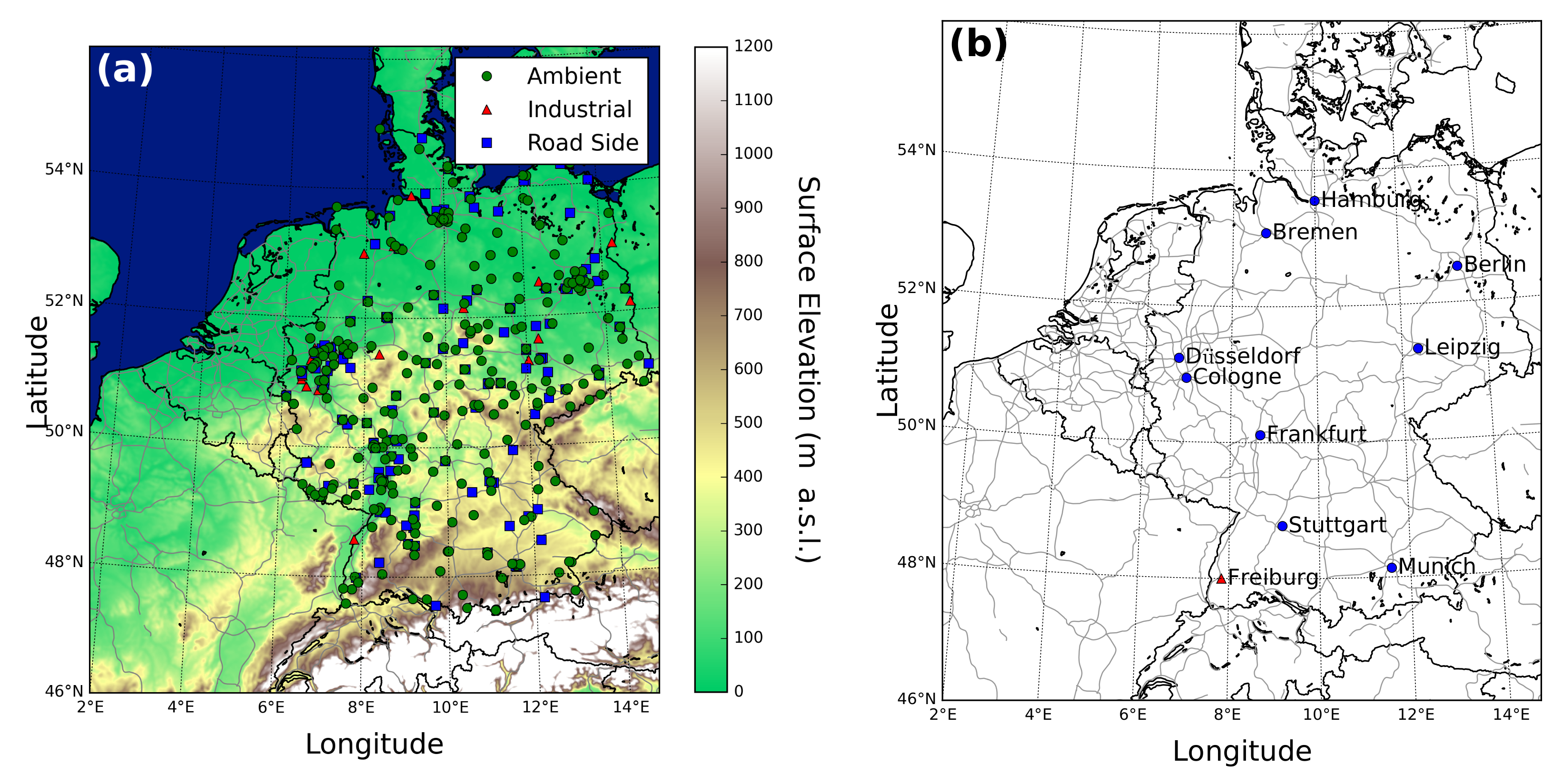
2.1. Study Area

This study focuses on Germany in the Central Europe. Germany is the fifth largest European Union member state by area with its territory covering 357,022 km

^{2}

. However, Germany has the largest population and gross domestic product (GDP) among all European Union member states, with over 83 million inhabitants [30] and 3800 billion US dollars GDP [31] in 2019. With high population density and heavily industrialized, Germany is facing a series of air pollution problems. Nitrogen oxides related air pollution is the most concerned issue among all air pollution problems in Germany. Although the NO

_{2}

load in Germany generally shows a decreasing trend, NO

_{2}

concentrations in many cities are still exceeding the World Health Organization (WHO) annual average limit of 40

µ

g/m

^{3}

. Such exceedances are recorded at about 40% of the traffic oriented monitoring stations [32], constituting one of the most severe air pollution problems in Germany.

2.2. TROPOMI Tropospheric NO $_{2}$ Columns

TROPOspheric Monitoring Instrument (TROPOMI) is a passive nadir viewing satellite borne push-broom imaging spectrometer on board the Copernicus Sentinel 5 Precursor (S5P) satellite. The satellite was launched on 13 October 2017 on a sun-synchronous orbit at an altitude of ∼824 km, with a local equator overpass time of 13:30 on ascending node. The instrument has 8 spectral bands covering ultraviolet (UV), visible (VIS), near infrared (NIR) and short-wavelength infrared (SWIR). The instrument takes measurements at 450 positions across the orbital track which cover a swath of ∼2600 km, providing daily global coverage observations. The spatial resolution of the instrument is 3.6 km (across-track) × 7.2 km (along-track) for measurements taken before 6 August 2019. Thereafter the instrument was switched to a better spatial resolution of 3.6 km (across-track) × 5.6 km (along-track). A more detailed description of the TROPOMI instrument can be found in Veefkind et al. [13].

Tropospheric NO

_{2}

columns measured by TROPOMI are used in this study for the estimation of surface NO

_{2}

concentration. The retrieval of tropospheric NO

_{2}

is briefly described as follows. NO

_{2}

slant column densities (SCDs) are derived from earthshine radiance spectra in the visible band from 405–465 nm using the differential optical absorption spectroscopy (DOAS) spectral retrieval technique [33]. Retrieved NO

_{2}

SCDs are then converted to vertical column densities (VCDs) using the concept of air mass factors (AMFs) [34]. The AMFs used for the retrieval of NO

_{2}

VCDs are calculated at 437.5 nm with NO

_{2}

vertical profiles taken from the global chemical transport model TM5-MP [35]. Albedo data used for AMF calculation is taken from the climatology albedo database derived from 5 years of Ozone Monitoring Instrument (OMI) satellite observations [36], which is advantageous due to the similar overpass time (13:30 local time) and viewing conditions with TROPOMI. Cloud parameters used for the calculation of AMF for cloud scene measurements are taken from the TROPOMI operational cloud product, which is retrieved by the OCRA/ROCINN algorithms [37,38]. Separation of stratospheric and tropospheric columns is achieved by using the STRatospheric Estimation Algorithm from Mainz (STREAM) [39]. STREAM is a modified reference sector method that does not require additional model input, and can be considered as a complement to the operational stratospheric correction based on data assimilation. A more detailed description of the tropospheric NO

_{2}

retrieval algorithm can be found in Liu et al. [40]. The retrieved tropospheric NO

_{2}

columns show good agreement with ground-based Multi-AXis Differential Optical Absorption Spectroscopy (MAX-DOAS) measurements with mean biases of −39% over Munich and −26 to −46% over polluted regions over the globe [40].

2.3. Ambient Air Quality Monitoring Station Data

Ambient NO

_{2}

concentrations data in Germany are acquired from air quality monitoring network operated by the Environment Agency of each Federal State (Landesamt für Umwelt, LfU) and summarized by the Federal Environment Agency (Umwelt Bundesamt, UBA) of Germany. The air quality monitoring network comprises 455 in situ monitoring stations, in which 268 of them are ambient stations, 30 of them are industrial stations and 157 of them are road side stations. Locations of all air quality monitoring stations are shown in Figure 1a. Locations of major cities are also indicated in Figure 1b. In this study, we only used data measured by ambient monitoring stations to avoid strong influences from very local sources, i.e., traffic and industrial. These monitoring stations cover both urban, suburban and rural areas of Germany. These air quality monitoring stations use in situ chemiluminescence NO

_{2}

analyzers to measure ambient NO

_{2}

concentrations. Details of the air quality monitoring network as well as air quality monitoring data can be found on the website of the European Environment Agency (https://www.eea.europa.eu/ accessed on 14 December 2020).

2.4. Meteorological Data

Several meteorological parameters are also used to improve the estimation of surface NO

_{2}

concentrations over Germany. In this study, meteorological parameters, such as, boundary layer height, surface air temperature, wind speed, relative humidity, precipitation and downward ultraviolet radiation, are taken from the European Center for Medium-Range Weather Forecasts (ECMWF) ERA5 reanalysis product [41]. The ERA5 reanalysis data covers a long time period, since 1979, and provides consistent meteorological data on a global scale. The reanalysis data are produced with a data assimilation scheme, which combined various measurements as prior information from model forecasts. The original ERA5 data set is in a spatial resolution of ∼31 km (T255 Spectral). The data are then transformed to the latitude-longitude coordinate system, with a horizontal resolution of 0.25

^{\circ}

× 0.25

^{\circ}

through the Copernicus Climate Change Service. The ERA5 reanalysis data is available on the Copernicus Climate Data Store (https://cds.climate.copernicus.eu accessed on 14 December 2020).

2.5. Surface Elevation Data

The territory of Germany stretches from the North Sea and the Baltic Sea across the Northern Lowland to the Alps in the South. The surface elevation of Germany ranges from sea level up to 2963 m above sea level (a.s.l.) with the highest point at Zugspitze. As the surface elevation of Germany varies in such a wide range, it is also an important factor for the estimation of surface level NO

_{2}

concentrations from satellite observations of vertical columns. In this study, surface elevation data from the Digital Elevation Model over Europe (EU-DEM) is used. EU-DEM is a digital surface model provided by the Copernicus Land Monitoring Service. It is a hybrid product produced from the Shuttle Radar Topography Mission (SRTM) [42] and Advanced Spaceborne Thermal Emission and Reflection Radiometer (ASTER) Global Digital Elevation Model (GDEM) [43] data using a weighted averaging approach. The spatial resolution of the EU-DEM data set is about 30 m. The surface elevation map of Germany and its surrounding areas is shown in Figure 1a.

2.6. Population Data

Geospatial distribution information of population is required for the investigation of NO

_{2}

exposure. In this study, the Gridded Population of the World (GPW) data set version 4 [44] obtained from the NASA Socioeconomic Data and Applications Center (SEDAS) (https://sedac.ciesin.columbia.edu/ accessed on 14 December 2020) is used. The gridded population data is in a resolution of 0.04

^{\circ}

× 0.04

^{\circ}

(∼5 km) and is available every 5 years. Population data from 2015 is used in this study and the population distribution across Germany is assumed to be static during the entire period from 2018 to 2020.

2.7. Regional Chemical Transport Model

In this study, Chemical Transport Model (CTM) POLYPHEMUS/DLR data are used to evaluate and compare our results to independently estimated surface NO

_{2}

concentrations. POLYPHEMUS/DLR is an operational regional CTM that provides daily forecast of air pollution over Europe on a routine base since 2014. The output data of the POLYPHEMUS model covering Europe (latitude of 34–60

^{\circ}

and longitude of −12–40

^{\circ}

) is in a horizontal resolution of 0.3

^{\circ}

(longitude) × 0.2

^{\circ}

(latitude) and a temporal resolution of 1 h. It covers the troposphere up to 12 km altitude with 20 vertical levels. The vertical resolution is 20 m near the surface, 50 m up to 200 m altitude, 100 m up to 1 km altitude and 1 km up to 12 km altitude. The data is freely available via Geospatial Web Services of the German Aerospace Center (DLR) (https://wdc.dlr.de/data_products/ accessed on 14 December 2020). The model implementation is based on the POLYPHEMUS platform [45]. Meteorological input parameters required for CTM simulations are taken from Weather Research and Forecasting (WRF) Version 3.5 [46] simulations with a spatial resolution of 30 × 30 km

^{2}

. The WRF simulation is initialized daily with Global Forecast System (GFS) data provided by the National Oceanic and Atmospheric Administration (NOAA). The original POLYPHEMUS simulation platform covers a wide range of atmospheric models. We use the Polair3D [47] model as the main driver for transport and chemistry. For the calculation of tropospheric trace gases and aerosols, the Regional Atmospheric Chemistry Modeling (RACM) chemical mechanism [48] is applied together with the SIze REsolved Aerosol Model (SIREAM) and Secondary ORGanic Aerosol Model (SORGAM) size-resolved aerosol model [49,50]. The direct space-time third-order advection scheme (DST3) [51] is used for transport simulation, while a second-order Rosenbrock method [52] is used for the calculation of atmospheric diffusion. Boundary conditions are extracted from a 10-year model run by the Model for OZone and Related chemical Tracers (MOZART) [53]. Vertical diffusion coefficients are calculated based on the Troen and Mahrt parameterization [54] from WRF forecasts. Dry deposition velocities for trace gases are derived following Zhang et al. [4]. Land cover characterization is taken from the US Geological Survey (USGS) data set, which is employed for calculating biogenic emissions. Anthropogenic emissions are taken from the TNO-MACC inventory [55,56] with base year 2005. Emissions were not updated for the time period used in this study, i.e., the actual emission trend is not taken into account. The POLYPHEMUS/DLR model has been developed within the PASODOBLE project [57] for mountainous terrain [58] and has been recently used to assess COVID-19 lock-down effect on surface NO

_{2}

[59].

3. Methodology

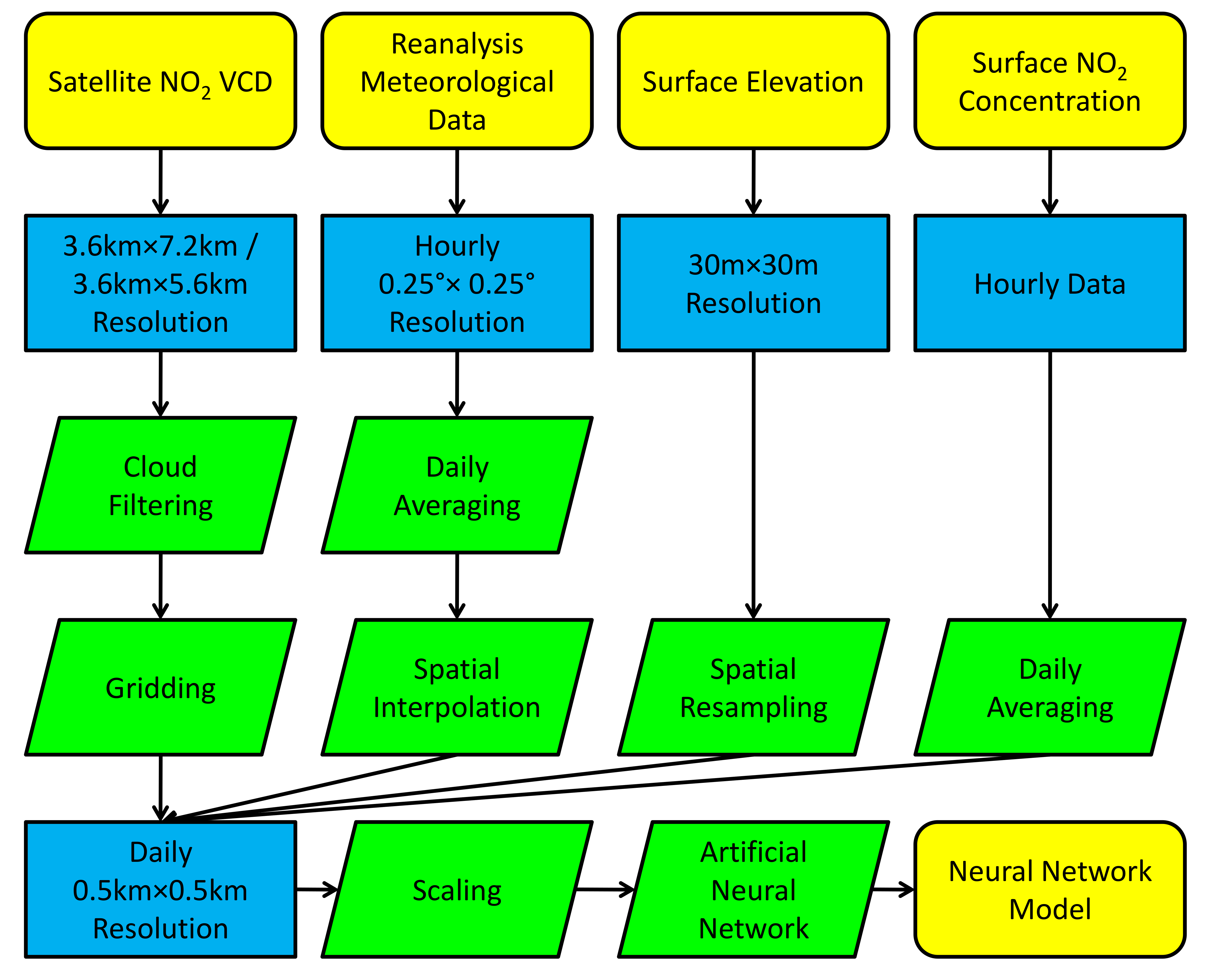
3.1. Data Preprocessing

All the data sets described in Section 2 are in different spatio-temporal resolutions. Therefore, it is necessary to preprocess the data to bring them onto a uniform spatio-temporal domain, so that these data can be paired up and used for the model training. In this study, we re-projected all data onto a grid of daily 0.5 km × 0.5 km over Germany. This spatial resolution is selected to strike a balance between having more accurate average value and capturing the fine scale gradient over complex terrain areas. Details of the preprocessing of each data set are presented in the following.

3.1.1. Regridding TROPOMI NO $_{2}$ Data

Ground pixels of TROPOMI measurements are irregular in shape and often multiple pixels overlap towards the ends of the orbits. To pair up the satellite NO

_{2}

data with other data sets, TROPOMI tropospheric NO

_{2}

columns are first regridded onto regular grid with spatial resolution of 0.5 km × 0.5 km. Satellite observations are insensitive to NO

_{2}

below clouds, and uncertainties of satellite observations under cloudy condition are much larger than that of clear sky measurements. Therefore, proper cloud filtering is necessary to avoid cloud contaminated data affecting following data analysis. To obtain a balance between having sufficient measurements while minimizing the influences of cloud contaminated data, only satellite data with cloud radiance fraction (

C R F

) of less than 50% are considered in the analysis. Measurement uncertainties related to cloud contamination are typically within 15% for observations with

C R F

smaller than 0.5 over polluted regions [40]. Therefore, the threshold of

C R F

of 0.5 is selected in this study. In addition to cloud filtering, we also excluded data with solar zenith angle larger than 85

^{\circ}

and root mean square of spectral fit residual larger than 0.001 in the following analysis.

In this study, we adopted a cloud weighting scheme in the gridding algorithm to further minimize effects due to clouds, by assigning a higher weight (W) to clear sky observations [60,61]. Gridded satellite NO

_{2}

columns (

V C D_{g r i d}

) are based on all tropospheric vertical column observations (

V C D

) within a certain time frame, i.e., a day. The weighted average is calculated for each grid cell with multiple overlapping satellite observations. The gridded NO

_{2}

column (

V C D_{g r i d}

) can be expressed by Equation (1).

V C D_{g r i d} = \frac{\sum_{i = 1}^{n} V C D_{i} \times W_{i}}{\sum_{i = 1}^{n} W_{i}} with W_{i} = \frac{1}{{(1 + 3 \times C R F_{i})}^{2}}

(1)

where

V C D_{g r i d}

is the gridded tropospheric NO

_{2}

column, while

V C D_{i}

represents each individual observation i overlapping with the grid cell. n is the total number of measurements overlapping with the grid cell within a certain time frame, i.e., a day. The weighting of each individual observation i is denoted as

W_{i}

, which is dependent on its cloud radiance fraction (

C R F_{i}

). The uncertainties of tropospheric NO

_{2}

columns related to cloud contamination are estimated following the function of (1 + 3 ×

C R F

). Therefore, the inverse square of this function is used as the weighting in the gridding process. Noted that although the satellite data is regridded onto a higher resolution grid of 0.5 km × 0.5 km, the original resolution of satellite measurement remains at 3.6 km × 7.2 km (or 3.6 km × 5.6 km after 6 August 2019). The relatively large satellite footprint might not be able to capture the strong spatial gradient of NO

_{2}

over small point sources, and results an underestimation over these pollution hotspots.

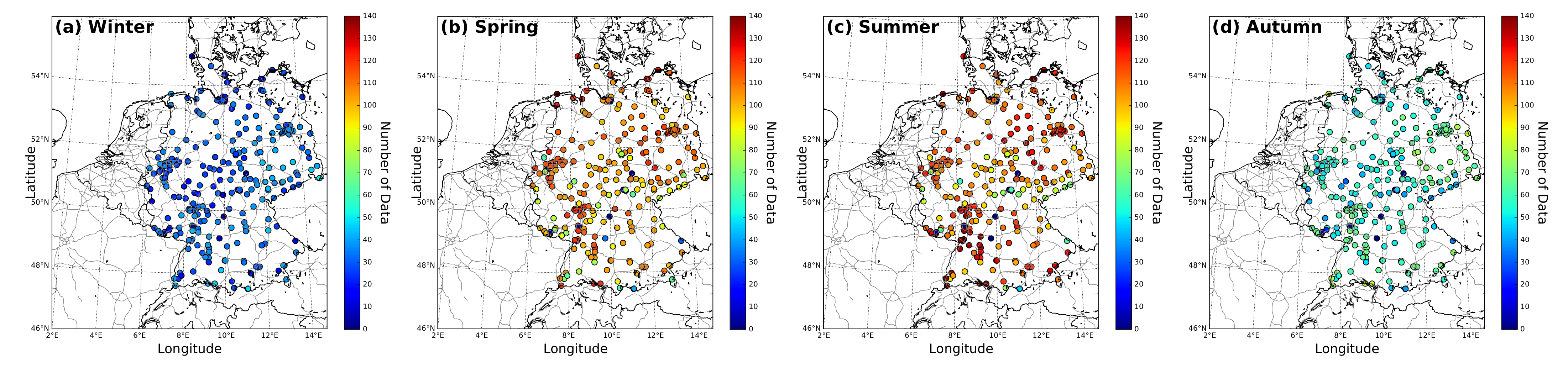
3.1.2. Preprocessing of Ambient Air Quality Monitoring Station Data

Ambient NO

_{2}

concentrations data acquired from the 268 monitoring stations are averaged to daily mean values for the model training. Data from each ambient air quality monitoring station is mapped on onto a 0.5 km × 0.5 km grid over Germany according to the measurement site locations. Daily averaged data instead of the instantaneous value measured during satellite overpass time are used in this study to avoid strong influences caused by very local or single incident during satellite overpass time. In addition, using daily averaged value would provide more representative surface NO

_{2}

concentration maps for the overall pollution conditions. According to the validation result (see Section 4.1), we believe that the neural network model is able to reproduce daily averaged NO

_{2}

concentrations using satellite observations at noon. Daily averaged in situ measurements are paired with satellite data at the corresponding grid of the same day. The paired data set is then used to train and validate the neural network model for the estimation of surface NO

_{2}

concentrations.

3.1.3. Interpolation of Meteorological Data

Meteorological parameters taken from ERA5 model are first averaged to daily data. Daily averaged meteorological parameters are then spatial bilinear interpolated to the 0.5 km × 0.5 km spatial grid over Germany (same as the regridded satellite). Daily averaged and spatially interpolated meteorological parameters are in a uniform spatio-temporal grid of daily 0.5 km × 0.5 km resolution. These data sets are then paired up with the satellite and in situ monitor observations of NO

_{2}

for the training and validation of the neural network model.

3.1.4. Resample of Surface Elevation Data

Surface elevation used in this study is taken from the EU-DEM data. The EU-DEM data set is in a spatial resolution of 30 m. To pair the surface elevation data with other data sets for the training and validation of the model, we resampled the surface elevation data to a spatial resolution of 0.5 km × 0.5 km (same resolution as the regridded satellite data). The resampling is simply achieved by calculating the mean elevation of each elevation point in the EU-DEM data set which falling within the grid cell. The resampled surface elevation data is then used in the following analysis.

3.1.5. Interpolation of Population Data

Population data is introduced for the approximation of NO

_{2}

exposure. The original population data set is in a resolution of 0.04

^{\circ}

× 0.04

^{\circ}

(∼5 km). We spatially bilinear interpolated the population data of 2015 to 0.5 km × 0.5 km resolution (same resolution as the regridded satellite data) over Germany. Socio-economical and mobility factors are not considered in the interpolation of population. The interpolated population data is then used for NO

_{2}

exposure approximation as introduced in Section 3.3.

3.1.6. Interpolation of Regional Chemical Transport Model Data

POLYPHEMUS CTM results are used to evaluate and compare the neural network estimation of surface NO

_{2}

concentrations. The original model output is in a horizontal resolution of 0.3

^{\circ}

(longitude) × 0.2

^{\circ}

(latitude) and a temporal resolution of 1 h. In this study, NO

_{2}

concentrations at the lowest layer (lowest 20 m) are first averaged to daily values and then spatially interpolated the data 0.5 km × 0.5 km resolution (same resolution as the regridded satellite data) over Germany using a bilinear interpolation algorithm. The resulting data set is then used as reference for the evaluation of the neural network model estimation.

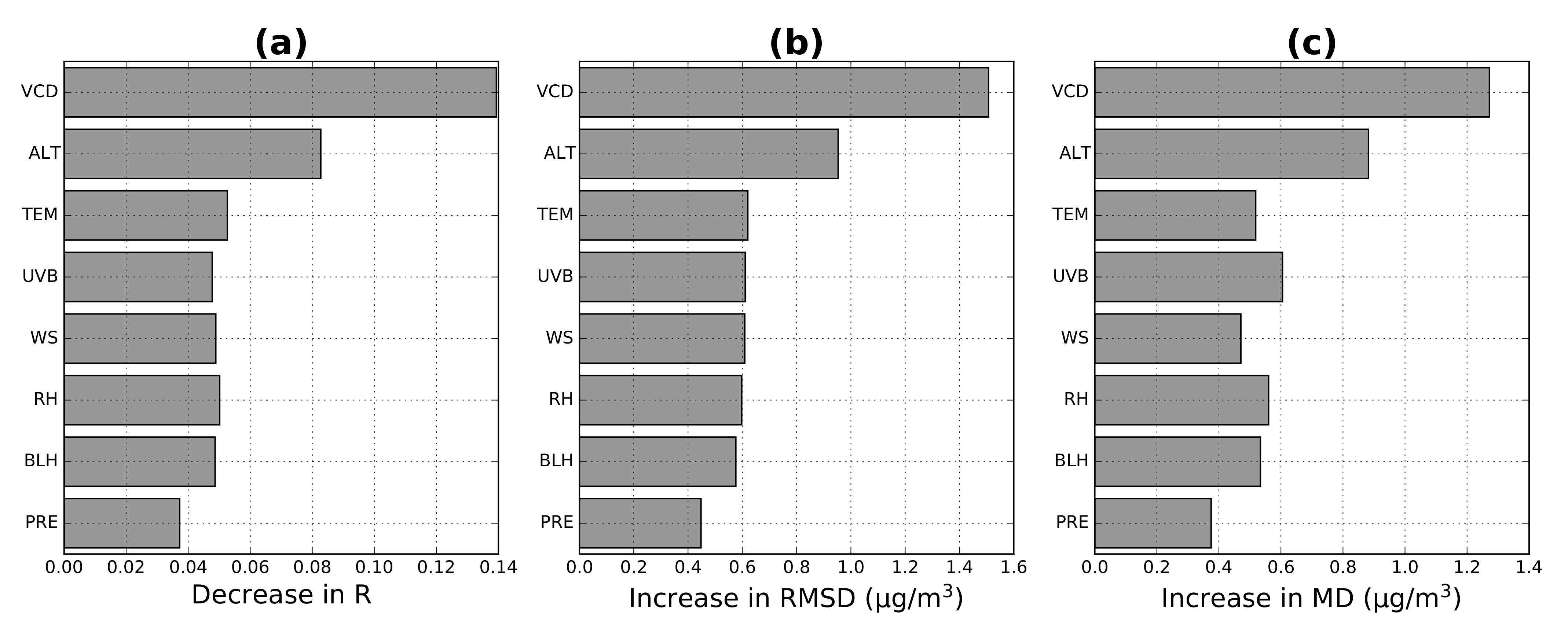
3.2. Machine Learning and Model Training

Machine learning approximates a function that represents the relationships between inputs and outputs data by both linear and non-linear regressions. In this study, we use the artificial neural network (refers as neural network (NN) from hereafter) to learn the non-linear relationships between inputs and outputs. The neural network model formulates surface NO

_{2}

concentrations as a function of all input parameters (see Equation (2)). Details of input and output parameters of the neural network model are listed in Table 1.

\begin{matrix} C O N C (x, y, t) = & f (V C D (x, y, t), B L H (x, y, t), T E M (x, y, t), W S (x, y, t), R H (x, y, t), P R E (x, y, t), \\ U V B (x, y, t), A L T (x, y, t)) \end{matrix}

(2)

where x and y represents the coordinate of the measurement, and t denotes the measurements time. Abbreviation of each parameter is listed in Table 1.

As mentioned in Section 3.1, tropospheric NO

_{2}

columns from TROPOMI are first filtered for clear sky data (

C R F

< 0.5) and regridded to 0.5 km × 0.5 km resolution for each day. Surface NO

_{2}

concentrations obtained from ambient air quality monitoring stations are first averaged to daily mean and then paired with satellite data at the corresponding grid. Daily averaged meteorological parameters taken from ERA5 reanalysis product are spatially interpolated to the same resolution as the regridded satellite. After regridding and interpolation, all parameters listed above are in a uniform spatio-temporal grid of daily 0.5 km × 0.5 km resolution. Coinciding data (with all 9 parameters available on the same grid on the same day) are paired up for the model training and validation. As the parameters listed in Table 1 are different in units and magnitudes, which could lead to unstable performance of the model. Therefore, we scaled all the parameters before using them for model training. The scaling of each parameter can be described by Equation (3).

x_{s c a l e d} = \frac{2 \times (x - x_{m i n})}{x_{m a x} - x_{m i n}} - 1

(3)

where x represents the unscaled data of each parameter listed in Table 1, i.e., VCD, BLH, TEM, WS, RH, PRE, UVB, ALT and CONC.

x_{s c a l e d}

is the scaled data.

x_{m i n}

and

x_{m a x}

denote the minimum and maximum value of the parameter. All scaled data lie between −1 and 1. The scaled data set is then used to train and validate the model.

The neural network model used in this study consists of 4 hidden layers. The number of neurons of the first to the last layer is 40, 20, 10, and 5, respectively. The model is trained using the stochastic gradient descent (SGD) algorithm with mean squared error (MSE) as loss function. Figure 2 shows the procedure and data flow for the training of the neural network model. We also tested other settings with more layers and number of neurons. However, the performance of the model does not show any significant improvement. Therefore, we use these settings to train the neural network model.

In total, there are 76,338 pairs of data available for training and validation. The number of available data pairs from 2018 to 2020 sorted for each season is shown in Figure 3. Relatively more data is available in spring and summer compared to winter and autumn. It is mainly due cloudiness in the cold months. The available data pairs are then randomly splitted into two groups, 90% of the data (68,704) are used for the training of the neural network model, the rest (7634) are used to validate the model.

In evaluating the model, we mainly rely on several statistical indicators, i.e., Pearson correlation coefficient (R), root mean square deviation (RMSD), mean bias (MB) and mean deviation (MD). R indicates the agreement between model and in situ data for validation. RMSD, MB and MD are measures of the differences between model results and in situ measurements of surface NO

_{2}

concentrations. The definition of RMSD, MB and MD are denoted by the following equations.

RMSD = \sqrt{\frac{\sum_{i = 1}^{n} {(f (x_{i}) - y_{i})}^{2}}{n}}

(4)

MB = \frac{\sum_{i = 1}^{n} (f (x_{i}) - y_{i})}{n}

(5)

MD = \frac{\sum_{i = 1}^{n} | f (x_{i}) - y_{i} |}{n}

(6)

where

f (x_{i})

is the model result,

y_{i}

indicates the in situ data used for model validation, and n represents the number of data used for validation.

3.3. Approximation of Annual Mean NO $_{2}$ Exposure

Air pollution risk on human health is a function of exposure to the pollutant. Air pollution exposure can be expressed for an individual, or for the entire population. Assessing NO

_{2}

exposures using in situ monitoring network data is likely to introduce large uncertainty mainly due to the spatial variation of NO

_{2}

cannot be captured by the sparsely distributed monitoring stations. In this study, we are looking into annually averaged NO

_{2}

exposure level for the entire population in Germany. Annual mean NO

_{2}

exposure level can be calculated using annual averaged NO

_{2}

concentration maps following Equation (7).

\bar{E} = \frac{\sum_{i = 1}^{n} c_{i} \times p_{i}}{\sum_{i = 1}^{n} p_{i}}

(7)

where

\bar{E}

is the annual mean NO

_{2}

exposure level for the entire population.

c_{i}

represents estimated annual mean NO

_{2}

concentration of grid i.

p_{i}

denotes the number of population of grid i. We assume the population distribution is static for the entire period from 2018 to 2020.

4. Results and Discussion

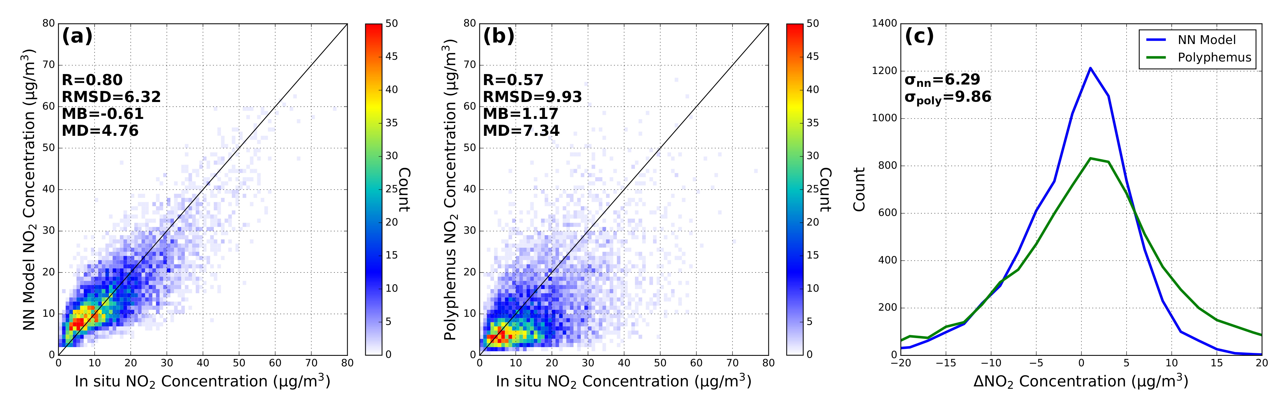
4.1. Validation and Comparison to CTM Predictions

The evaluation of the trained neural network model for the estimation of surface NO

_{2}

concentrations is performed by comparing modeled outputs with the corresponding data sets described in Section 3.2. To also allow the comparison of neural network model results to CTM forecasts, we additionally compared the POLYPHEMUS CTM forecasts of surface NO

_{2}

concentrations to the validation data set. A scatter plot of neural network model predicted surface NO

_{2}

concentrations against in situ measurements is shown in Figure 4a, while Figure 4b shows the scatter plot of POLYPHEMUS forecast against in situ measurements. Figure 4c shows the histogram of NO

_{2}

concentration from neural network and POLYPHEMUS results compared to in situ measurements. The comparison of neural network model result in in situ measurements shows very good agreement with R of 0.80, RMSD of 6.32

µ

g/m

^{3}

, MB of −0.61 ± 6.29

µ

g/m

^{3}

and MD of 4.76

µ

g/m

^{3}

. While the comparison of POLYPHEMUS forecast to in situ measurements results in R of 0.57, RMSD of 9.93

µ

g/m

^{3}

, MB of 1.17 ± 9.86

µ

g/m

^{3}

and MD of 7.34

µ

g/m

^{3}

. These numbers are in-line with other model results on the European scale (e.g., Ciarelli et al. [62], Wahid et al. [63]) that neural network models can outperform CTM forecasts. Our neural network model gives 0.23 higher R and ∼35% lower RMSD, MB and MD compared to the CTM. The neural network predictions of surface NO

_{2}

concentrations on average show a deviation of 4.76

µ

g/m

^{3}

from the measurement. The neural network on average underestimates surface NO

_{2}

concentrations by 0.61

µ

g/m

^{3}

, while POLYPHEMUS model generally overestimated NO

_{2}

levels by 1.17

µ

g/m

^{3}

. The negative bias of the neural model predictions is partly related to cloud filtering in the satellite data processing. Previous study shows that excluding observations with significant cloud coverage can result underestimating NO

_{2}

levels by 12–40% [64]. However, this clear sky bias is inevitable for satellite observations.

As expected, the neural network model performs better than CTM simulations when data coverage is sufficient. One has to note that both database and methodology used are completely different. The neural network model retrieves surface NO

_{2}

concentrations from actual satellite observations, meteorological and geographical information using a regression method. While the CTM predicts NO

_{2}

concentrations by simulating relevant physical and chemical processes in the troposphere. During the day, in the boundary layer, NO

_{2}

concentrations strongly depend on respective emission rates, calculated from an annual emission database that takes into account appropriate emission and activity factors, e.g., for the traffic sector. Part of the positive bias can be explained by the 2005 emissions database used in the CTM. Previous study using TNO MACC II emissions over Germany shows the NO

_{2}

concentrations were underestimated by 10–30% depending on location [56]. As these calculated emissions are only an approximation of the actual conditions, deviations from the measured NO

_{2}

concentrations have to be expected. On the other hand, the neural network model can better match the actual situation by using the latest satellite observations and reanalysis meteorological data, provided that coverage of day-to-day variations of NO

_{2}

is sufficient. In addition, the rather coarse spatial resolution of the CTM can induce averaging and spatial mismatch errors, which might further deteriorate the agreement with in situ monitor data.

To investigate the model performance only using instantaneous in situ and meteorological data during satellite overpass time, we also trained and validated the model with in situ monitor data and reanalysis meteorological data during satellite overpass time (±1.5 h). Neural network model trained with satellite overpass time data shows lower R of 0.76, larger RMSD of 8.22

µ

g/m

^{3}

and MD of 5.97

µ

g/m

^{3}

, while MB remain similar of −0.57

µ

g/m

^{3}

. larger deviation indicated that using the instantaneous data during satellite overpass time can be strong influenced by very local or single incident, and results more scattered outliers.

We also looked into the sensitivity of each fitting parameter used in the neural network model. Figure 5 shows the changes of Pearson correlation coefficient (R), root mean square of deviation (RMSD) and mean deviation (MD) caused by removing the variable from the neural network model. TROPOMI satellite observations of tropospheric NO

_{2}

vertical column density (VCD) is the most important parameter for the retrieval of surface NO

_{2}

concentrations. Despite the high uncertainties of satellite NO

_{2}

observations (up to 50%) [6], satellite observations provide columnar information of atmospheric NO

_{2}

which is strong correlated to the surface NO

_{2}

concentrations. Therefore, it is as expected to be the most important variable in the model. Although satellite NO

_{2}

observations play the most important role in predicting surface NO

_{2}

concentrations, the model is still performing considerably good with only using meteorological data and results R of 0.66. Training the neural network model with only meteorological inputs is similar to the statistical approaches which use meteorological data for air quality prediction. These models are reported doing reasonably well in air quality prediction, especially over areas with rather constant emissions [65,66,67]. The second most important variable is surface elevation (ALT). The surface elevation of Germany varies in a wide range (up to 2963 m a.s.l.) and it strongly affects the columnar NO

_{2}

amount. Therefore, it is an important factor for the retrieval of surface NO

_{2}

concentrations over areas with large variation of surface elevation. Other important factors affecting the surface NO

_{2}

concentration retrieval are seasonal variation (represented by air temperature (TEM) and relative humidity (RH)), dispersion (represented by wind speed (WS) and boundary layer height (BLH)) and photochemistry (represented by shortwave radiation (UVB)). The result also shows that precipitation (PRE) has only a very minor effect on surface NO

_{2}

concentrations, which reflects the fact that wet deposition is not the major removal pathway of atmospheric NO

_{2}

.

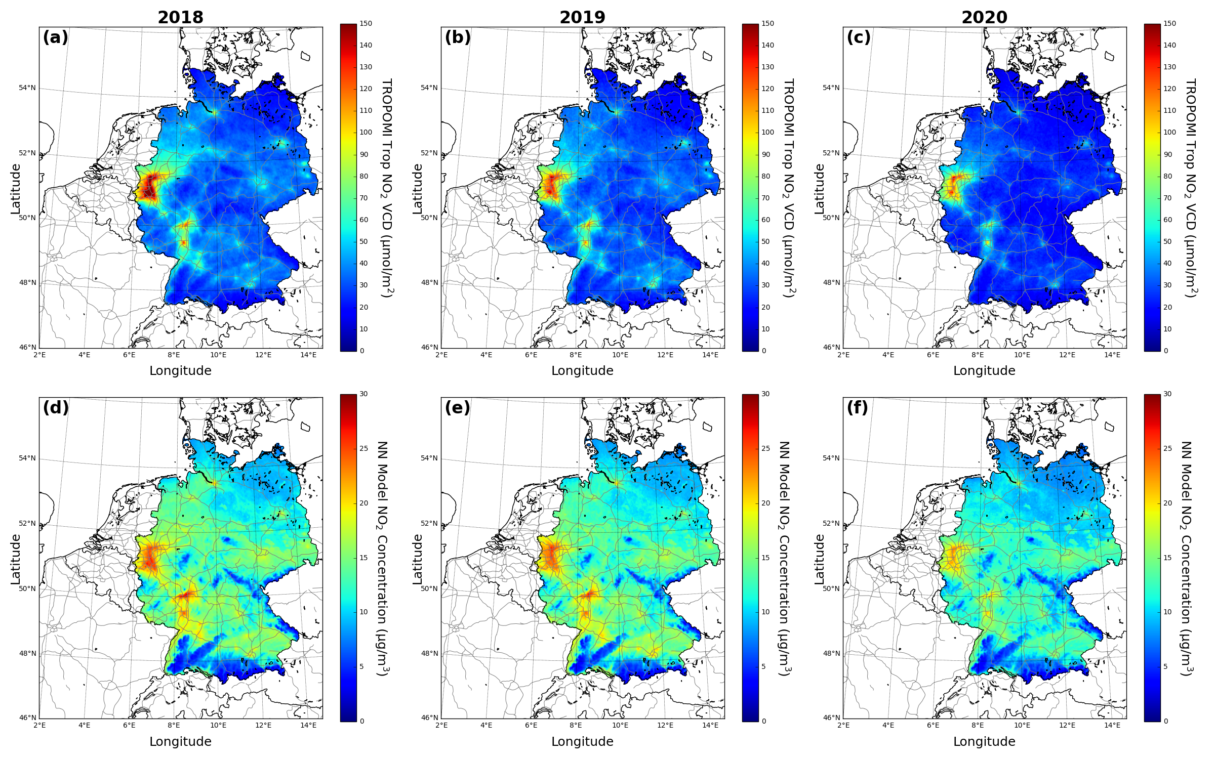
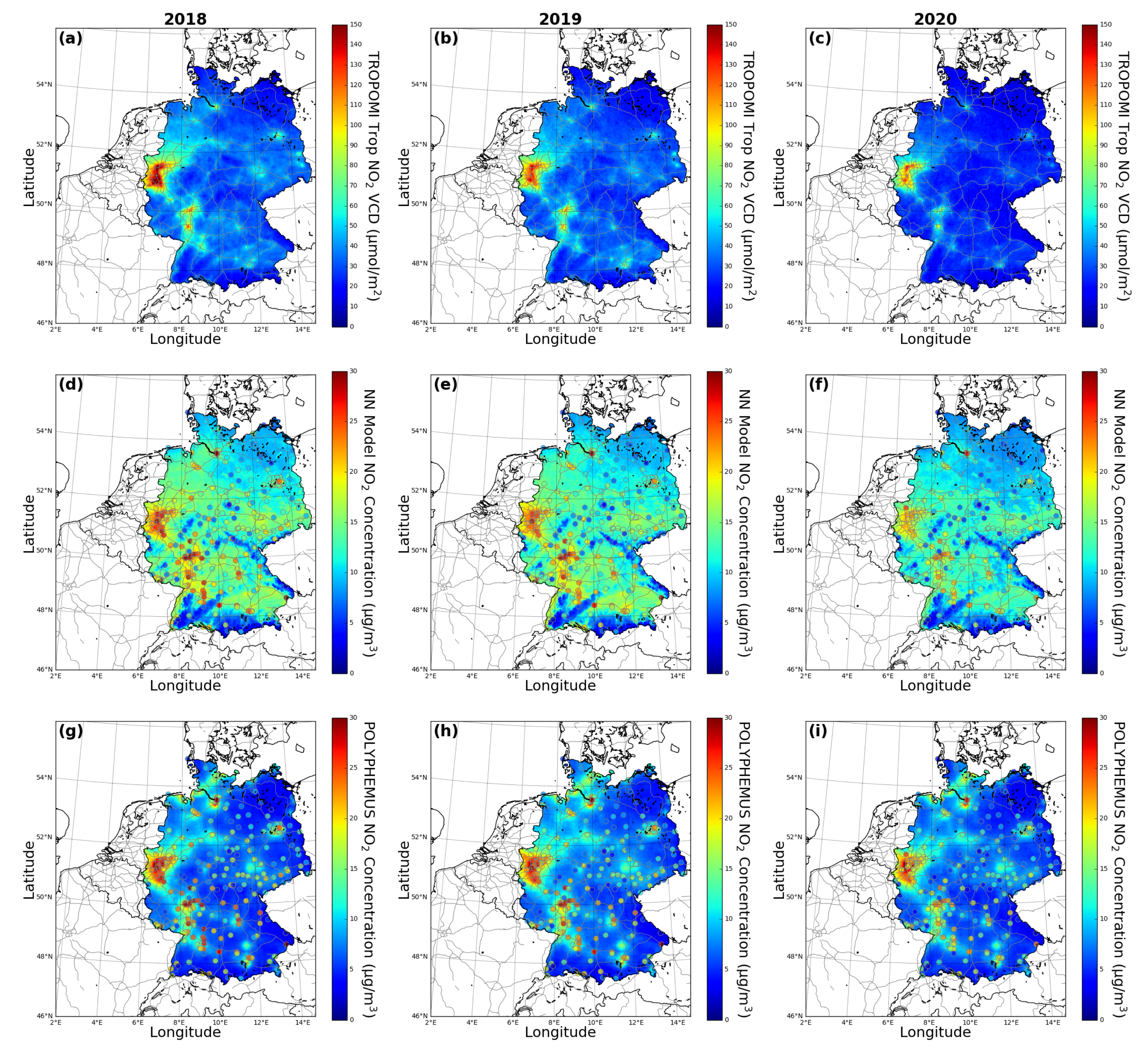
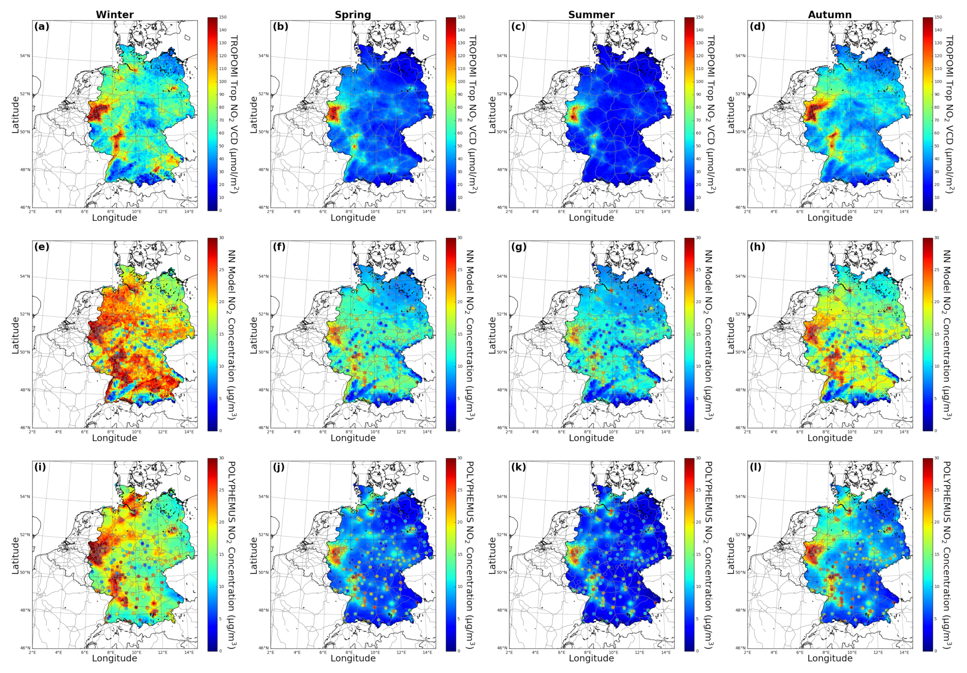
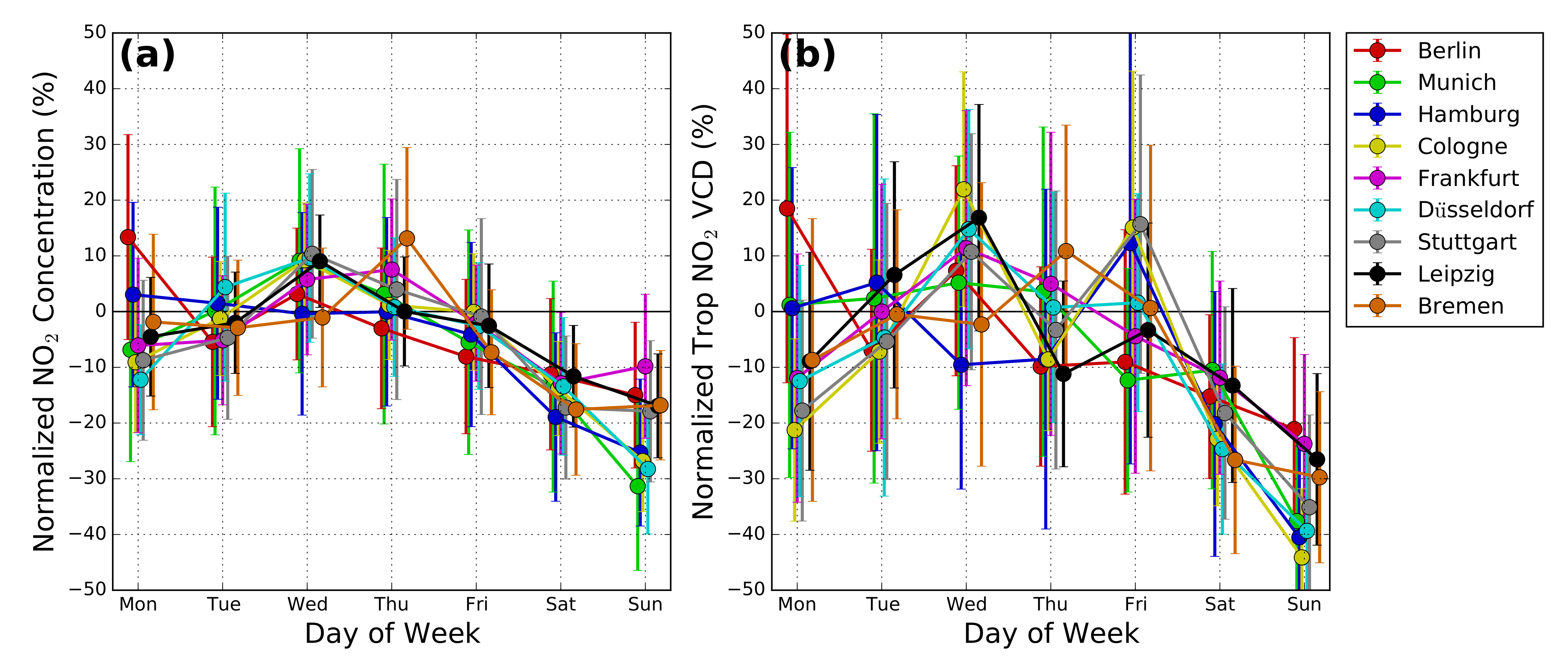
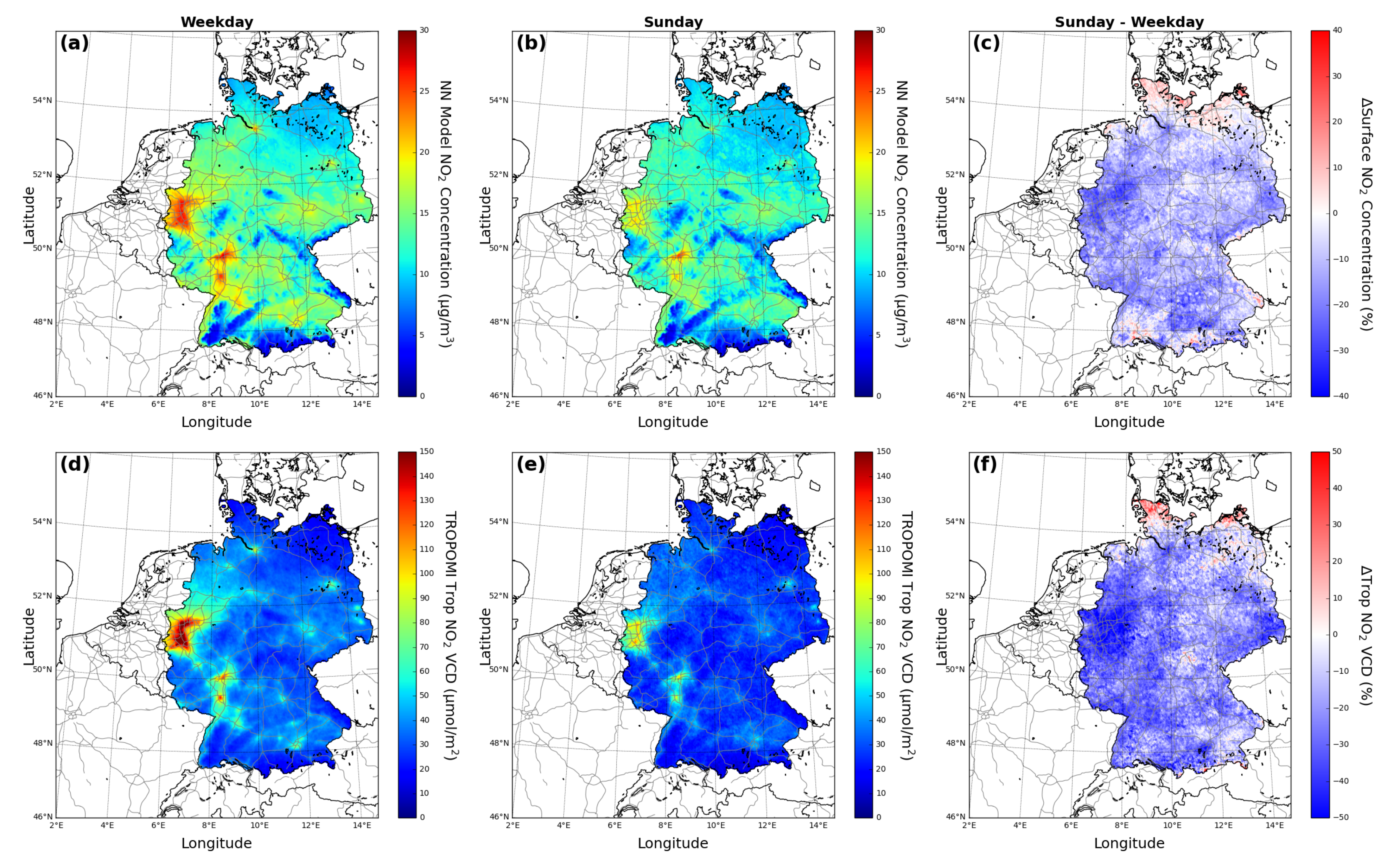
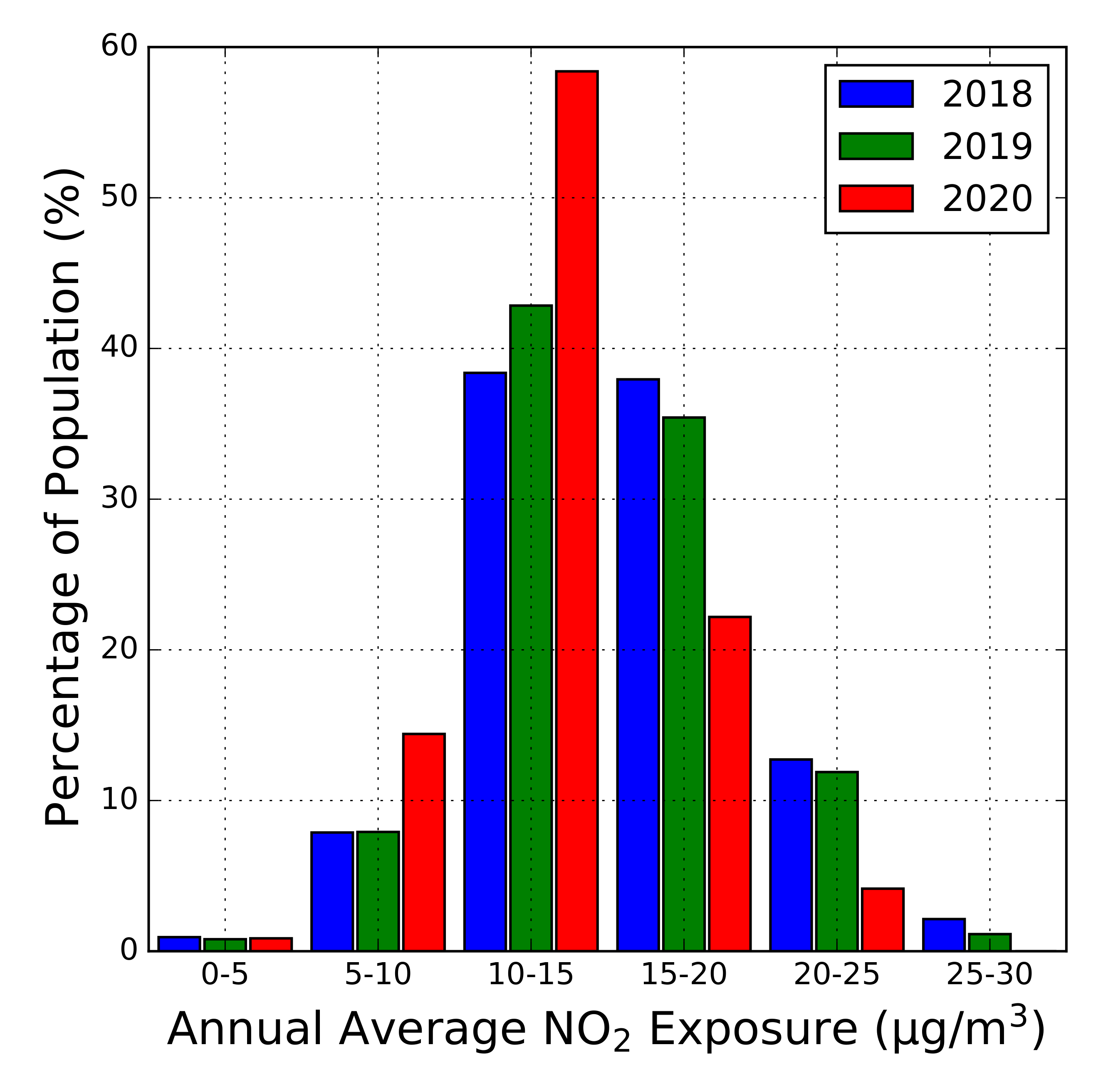
4.2. Spatio-Temporal Variations of Surface Level NO $_{2}$

Figure 6 illustrates the annually averaged spatial distribution of NO

_{2}

over Germany from 2018 to 2020. TROPOMI observations of tropospheric NO

_{2}

columns, surface NO

_{2}

concentrations retrieved by the neural model and POLYPHEMUS CTM simulations are shown. Corresponding in situ measurements of surface NO

_{2}

concentration are also indicated in Figure 6d–i. The NO

_{2}

levels generally show a small reduction in 2019 compared to 2018. Stronger reduction of surface NO

_{2}

concentrations as well as tropospheric columns can be observed in 2020, especially over urban areas, e.g., the lower Rhine region. The reduction of NO

_{2}

levels in 2020 is likely related to the COVID-19 pandemic (see Section 4.4). All three data sets show very similar spatial distribution of NO

_{2}

for 2018 and 2019. Higher levels of NO

_{2}

are observed in most of the population dense cities and industrial regions, e.g., the lower Rhine region, Frankfurt, Mannheim, Berlin, Hamburg, and Munich. These spatial patterns agree with the in situ monitoring data. Compared to POLYPHEMUS model simulations, the neural network model generally predicts higher values in most of the rural areas, which are more in line with in situ measurements. In addition, the neural network model is also performing better over regions with complex terrain, i.e., large variation of surface elevation over a small area. This is mainly related to higher spatial resolution of the neural network model that reduces the spatial averaging effect. Monitor stations at higher altitudes generally show lower NO

_{2}

concentrations, and this feature is well reproduced by the neural network model. For example, there are two monitor stations within 10–20 km of Freiburg (location indicated in Figure 1b) with altitudes about 700–900 m higher than other stations surrounding the city. NO

_{2}

concentrations reported from these two stations are much lower than other low altitude stations in this area. This altitude dependency is significant and that also explains why surface elevation is important in the neural network model as demonstrated in Section 4.1.

Seasonal variations of NO

_{2}

spatial distribution are shown in Figure 7. Data from 2020 is not used in the calculation of seasonal average to avoid influence from the large scale lockdown in Europe related to the COVID-19 pandemic in 2020. A more detailed analysis of COVID-19 impacts on the NO

_{2}

level is presented in Section 4.4. Pronounced seasonal variations of NO

_{2}

levels can be observed from all three data sets, with peak NO

_{2}

values in winter and lower NO

_{2}

levels in spring and summer. Higher NO

_{2}

levels during cold seasons are due to increase of energy consumption and emissions related to domestic heating. In addition, the atmospheric lifetime of NO

_{2}

is longer in winter, because of lower rate of photolysis, and more pronounced accumulation of NO

_{2}

are found during stagnant conditions. Shallower boundary layer height in cold months can also reduce the dispersion of NO

_{2}

near emission sources, which would increase near surface NO

_{2}

concentrations. This has been demonstrated in the sensitivity analysis in Section 4.1. The spatial distribution of surface NO

_{2}

concentration derived by the neural network and POLYPHEMUS model shows different characteristics. We observed that NO

_{2}

concentrations estimated by the neural network model show higher level of NO

_{2}

in rural (less polluted) areas which agree better with in situ monitor data compared to POLYPHEMUS simulations. The POLYPHEMUS model simulation of NO

_{2}

is mostly concentrated over population dense cities and industrial regions where the prescribed anthropogenic emissions are high, while significantly underestimated NO

_{2}

levels in rural areas. The underestimation of NO

_{2}

levels in rural areas is probably related to emission inventories used in the CTM which assign too low emissions over these areas. This underestimation is especially significant during winter, thus neural network model reaches an improved performance over CTM.

Human activities usually fall into a seven day weekly cycle. Reduction of industrial activities as well as traffic volume during the weekend leads to lower levels of pollutant emission, and this is known as the weekend effect [68]. Therefore, we analyzed the weekly pattern of NO

_{2}

for 9 major cities in Germany. Figure 8 shows the normalized mean weekly cycle of NO

_{2}

for 9 major cities in Germany. Retrieved surface NO

_{2}

concentrations within 5 km of the center of these cities are considered in the analysis. Data is normalized by subtracting and dividing by the corresponding mean weekday value (Monday to Friday). Both surface NO

_{2}

concentrations retrieved with the neural network model and TROPOMI observations of tropospheric NO

_{2}

column are shown. To avoid abnormalities caused by the large scale lockdown related to the corona virus pandemic in 2020, we excluded 2020 data from the weekend effect analysis. The locations of these nine cities are indicated in Figure 1b. Both surface NO

_{2}

concentrations and tropospheric columns show lower values during weekend. Surface NO

_{2}

concentrations are generally reduced by 10–30% on Sunday. Larger reduction of 20–45% can be observed from the tropospheric column observations. Our result is similar to the MAX-DOAS measurement study that stronger weekend reduction is observed in columnar NO

_{2}

measurements compared to surface concentrations [6]. Stronger weekend effect is observed in Munich, Düsseldorf, Cologne and Humburg, with 25–30% reduction of surface NO

_{2}

levels and 35–45% reduction of NO

_{2}

columns on Sunday. The weekend effect is less significant in Berlin, Bremen, Frankfurt and Leipzig, with surface and columnar NO

_{2}

reduced by 10–20% and 20–30% on Sunday. Due to the absence of weekend effects within natural emissions, the reduction of NO

_{2}

levels during weekend implies significant contributions of anthropogenic emissions in these cities. More insights of the spatial information of the weekend reduction effect is shown in Figure 9. The data shows a clear weekend reduction effect in both urban and rural areas of Germany. Nationwide, surface NO

_{2}

concentrations and tropospheric NO

_{2}

columns on Sunday reduced by 11% and 21%, respectively. Stronger weekend reduction of NO

_{2}

level can be observed over industrial and population dense regions, e.g., the lower Rhine region.

4.3. Application of NO $_{2}$ Exposure Approximation

As NO

_{2}

is harmful to human health, it is important to assess the population exposure levels instead of just the concentrations. The annual average (or areal average) of surface NO

_{2}

level over Germany is 12.79, 12.60 and 11.15

µ

g/m

^{3}

for 2018 and 2020, respectively. Noted that the neural network predictions on average show a negative bias of 0.61

µ

g/m

^{3}

. Therefore, the actually values might be higher than our estimations by ∼5%. The population density is typically higher in urban areas where the pollution levels are also heavier. Therefore, the average NO

_{2}

exposure level (or population average) is more relevant for the assessment of health impacts. The average NO

_{2}

exposure level can be calculated by multiplying surface NO

_{2}

concentration with population of the corresponding grid and then dividing by the total population. The national average NO

_{2}

exposure level for 2018 and 2020 is 15.53, 15.24 and 13.27

µ

g/m

^{3}

, respectively. The NO

_{2}

exposure level is generally about 25% higher than the average surface NO

_{2}

concentration. The results reflects the fact that there are more people living in urban areas where the pollution levels are expected to be higher. Therefore, reducing the ambient NO

_{2}

levels in population dense areas certainly helps to reduce the national exposure level. In addition to average exposure level, we also looked into the population distribution of different NO

_{2}

exposure levels for 2018 and 2020 (see Figure 10). The population NO

_{2}

exposure distribution of 2018 and 2019 is very similar. The result shows that only ∼8% of the total population is living in rather clear areas (annual average NO

_{2}

concentration below 10

µ

g/m

^{3}

). About 75–80% of the population is living in moderate polluted areas (annual average NO

_{2}

concentration between 10 and 20

µ

g/m

^{3}

), and ∼15% of the population is living is relatively polluted areas (annual average NO

_{2}

concentration above 20

µ

g/m

^{3}

). As the NO

_{2}

pollution level of Germany has been improved in 2020 (partly related to the COVID-19 pandemic, see Section 4.4), the exposure distribution has also changed significantly. About 15% of the total population is living in rather clear areas, ∼80% of the population is living in moderate polluted areas, and only less than 5% of the population is living is relatively polluted areas. Noted that the exposure calculation is just a rough estimation which does not consider the socio-economical and mobility factors, i.e., some people might be living in rural areas and commute to urban or industrial areas for work and relocation out of urban areas due to the COVID-19 pandemic. Looking into the health impacts related to NO

_{2}

exposure would be very meaningful. However, the epidemiologic literature on health effects of NO

_{2}

is still less exhaustive, and lacks of risk estimations for several outcomes that have been associated with other air pollutants. Thus, it is very difficult to assess the actual health impacts without full understood their cross-correlation. In addition, the assessment of health impacts related to NO

_{2}

exposure in Germany is beyond the scope of this study. Therefore, we decided to leave it for the future study.

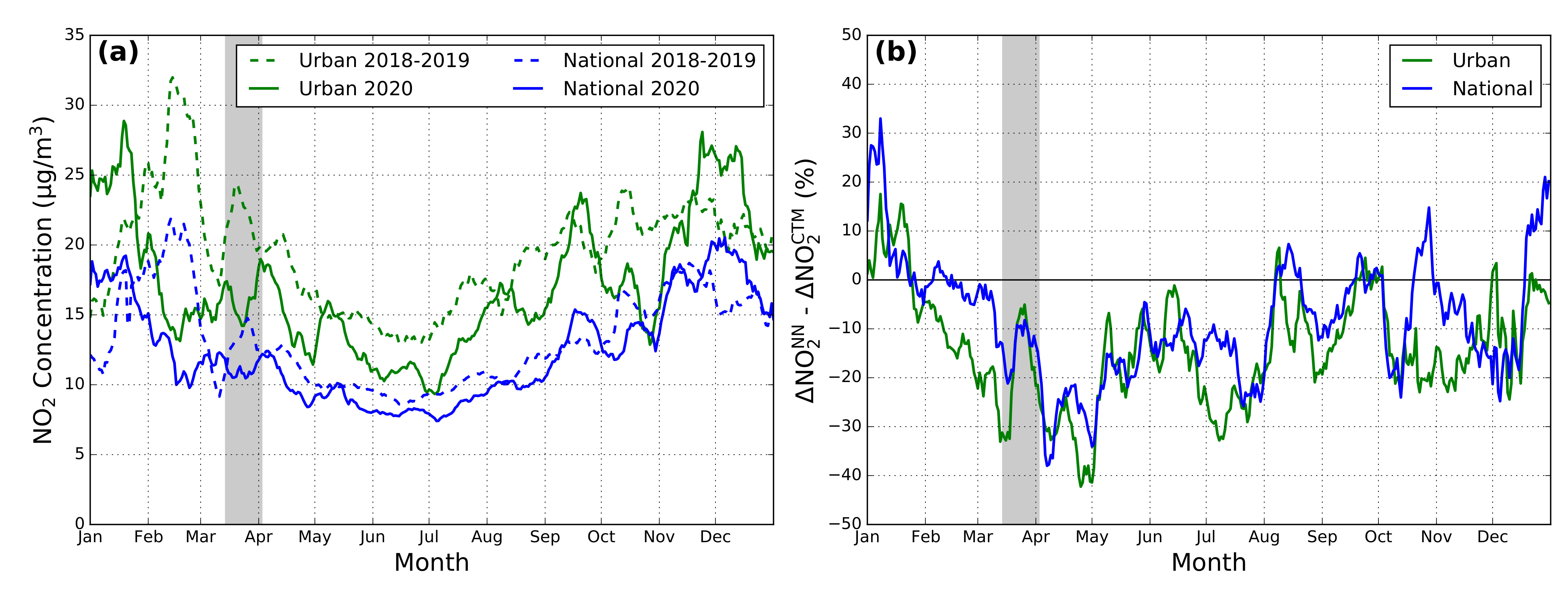
4.4. Impacts of COVID-19 Pandemic on Surface NO $_{2}$ Concentrations

A new type of infectious pneumonia was first identified in late December 2019 in the city of Wuhan, China, and was later spread all over the world and caused tremendous damage to the economy and loss of human life. This disease was later renamed by the World Health Organization (WHO) as coronavirus disease 2019 (COVID-19) on 11 February 2020. In response to the WHO declaration of global pandemic on 11 March 2020 [69], many countries, including Germany, have enforced lockdown measures by restricting people activities to reduce the spread of the virus. These lockdown measures have greatly changed human activity patterns and consequently caused impacts on pollutant emissions as well as air quality. The impacts of COVID-19 pandemic on air quality have been reported in many studies [70,71,72,73,74,75]. Therefore, we restricted the focus of this study to the corresponding impacts on NO

_{2}

levels in Germany. Figure 11a shows the time series of averaged surface NO

_{2}

concentrations over Germany (national) and nine major cities (urban). The geolocation of these nine selected cities are marked in Figure 1b. Averaged NO

_{2}

values of 2018–2019 are also shown for reference. To reduce the influence caused by weekend effect, 7-days moving average values are used in the analysis. Both national averaged and urban surface NO

_{2}

concentrations generally show lower values compared to data in 2018–2019 after the outbreak of COVID-19 in March 2020. Nationwide, 5–15% reduction can be observed from the surface NO

_{2}

concentrations, while the reduction in urban areas varies in a wider range of up to 30%. As the emissions data used in POLYPHEMUS CTM simulation remain unchanged during the entire study period, the change of NO

_{2}

concentrations in 2020 predicted by the CTM can be assumed to be purely meteorological driven. Therefore, the POLYPHEMUS CTM simulation can be used as reference to separate meteorological and anthroprogenic effects. The percentage change of surface NO

_{2}

concentrations predicted by CTM in 2020 compared to 2018–2019 (

Δ

NO

_{2}^{C T M}

) is considered as the meteorological contributions, while the percentage change of surface NO

_{2}

concentrations predicted by the neural network model (

Δ

NO

_{2}^{N N}

) consists both meteorological and anthropogenic effects. The anthroprogenic contribution on NO

_{2}

concentrations in 2020 can then be calculated by subtracting

Δ

NO

_{2}^{C T M}

from

Δ

NO

_{2}^{N N}

. The advantage of looking into the relative reduction instead of absolute reduction is that the bias the neural network estimation is canceled out. Figure 11b shows the anthroprogenic contribution to the change in surface NO

_{2}

concentrations in 2020 over Germany (national) and nine major cities (urban). Significant anthroprogenic impacts can be observed in both national average and urban data, especially after the outbreak of COVID-19 in Europe in March. During the first COVID-19 pandemic peak in March to May 2020, the relative reduction of NO

_{2}

level due to change in human activity is on average ∼20%, while stronger reduction effects are observed over urban areas. The corresponding reduction effect is then gradually decreased with the improvement of pandemic situation in summer.

To analyze the impact of COVID-19 in more detail, we looked into NO

_{2}

maps for the period right after WHO declared a global pandemic. Figure 12 shows weekly averaged NO

_{2}

maps for the period right after WHO declared a global pandemic. Averaged NO

_{2}

levels of March 2018–2019 are also shown for reference. Both surface NO

_{2}

concentrations and tropspheric columns are shown. From 14–20 March 2020, the government has announced a series of measures to reduce the spread of the virus, including closing schools, non-essential businesses and facilities, implementing border control and canceling entertainments and other big events. The NO

_{2}

levels during this period have already been reduced by ∼20% compared to the same time of the year in 2018 and 2019. Larger reduction of NO

_{2}

levels of ∼30% can be seen in the following week (21–27 March 2020) when the government implements stricter restriction measures, including curfew. However, a rebound of NO

_{2}

levels can be observed from 28 March to 3 April 2020. The drop and rebound of NO

_{2}

levels are likely related to the sudden stop of most commercial activities including logistic, which cause a demand and supply gap of consumable commodities. The logistic system is then slowly adapting to the new practice and catching up the supply for daily needs. After the first few weeks that WHO declared a global pandemic, people seem to have adapted to a new life style, e.g., working from home if possible, online teaching and learning, the NO

_{2}

level in Germany is constantly lower than the same period of the year compared to 2018 and 2019. The results illustrated that impacts of the COVID-19 pandemic on our daily life as well as on air quality. We successfully demonstrated the detection of anthropogenic impacts on air quality by combining satellite observations, machine learning and CTM simulations. This approach can also be used to assess the effectiveness of environmental protection measures in the future.

5. Conclusions

In this study, we developed a machine learning approach to estimate surface NO

_{2}

concentrations through the synergistic use of satellite observations over Germany. A neural network model is used to approximate the relationships between tropospheric NO

_{2}

columns, meteorological parameters and surface NO

_{2}

concentrations. TROPOMI satellite observations of tropospheric NO

_{2}

columns, meteorological parameters from ERA reanalysis product and ground-based in situ air quality monitoring network measurements are used for the training of the neural network model. The neural network model estimations of surface NO

_{2}

concentrations show good agreement with the validation data set, with Pearson correlation coefficient (R) of 0.80 and root mean square of deviation (RMSD) of 6.32

µ

g/m

^{3}

. Comparisons also show that the developed neural network model calculations are more accurate than regional CTM simulations. Sensitivity analysis show that satellite observations of NO

_{2}

columns and surface elevation data are the most important parameters, followed by air temperature, wind speed and shortwave radiation.

The developed neural network model is used to estimate surface NO

_{2}

concentrations over Germany from 2018 to 2020. Estimated surface NO

_{2}

concentrations are used to investigate the spatio-temporal characteristics, such as seasonal and weekly variations. Higher NO

_{2}

values are observed over population dense and industrial areas, e.g., the lower Rhine region, Frankfurt, Mannheim, Berlin, Hamburg, and Munich. Strong weekly variations can also be observed over these areas with reduction of NO

_{2}

level of 10–45% on Sunday, indicating the large contribution of anthropogenic emissions. The surface NO

_{2}

data set is also used to estimate NO

_{2}

exposure level in Germany. We estimated the annual average NO

_{2}

exposure for the entire population of Germany for 2018, 2019 and 2020 is 15.53, 15.24 and 13.27

µ

g/m

^{3}

, respectively. While the annual average NO

_{2}

concentration of 2018, 2019 and 2020 is only 12.79, 12.60 and 11.15

µ

g/m

^{3}

. The population distribution of NO

_{2}

exposure level indicates that generally over 85% of the population is living in low to moderate polluted areas (annual average NO

_{2}

concentration below 20

µ

g/m

^{3}

).

In 2020, the COVID-19 pandemic had a big impact on human activities as well as air quality. We investigated the impacts of the COVID-19 pandemic on ambient NO

_{2}

levels in Germany using the retrieved surface NO

_{2}

data sets. Combining with CTM simulation, we estimated that the reduction of surface NO

_{2}

concentrations of 10–30% in March 2020 is related to anthropogenic impacts, indicating the impacts of a series of restriction measures to reduce the spread of the virus. More detailed analysis also show different reduction levels in response to different control measures implemented by the government. Our results illustrated that the estimated surface NO

_{2}

data sets can be used in many aspects including exposure estimation and analysis of the COVID-19 effect on air quality. It also provided additional information of NO

_{2}

spatial distribution and potentially contribute to the future health exposure studies and political decisions on environmental protection.

Author Contributions

Conceptualization, K.L.C. and P.V.; methodology, K.L.C.; software, K.L.C.; validation, K.L.C.; formal analysis, K.L.C.; investigation, K.L.C.; resources, K.L.C., E.K., F.B. and S.L.; data curation, K.L.C.; writing–original draft preparation, K.L.C.; writing–review and editing, K.L.C.; visualization, K.L.C.; project administration, K.L.C., F.B. and P.V.; funding acquisition, P.V. and F.B. All authors have read and agreed to the published version of the manuscript.

Funding

This research was funded by Federal Minister of Transport and Digital Infrastructure (BMVI) within the framework of the mFUND research initiative (grant no. 19F2065).

Data Availability Statement

The TROPOMI tropospheric NO

_{2}

columns over Germany used in this study are publicly available at the German Aerospace Center (DLR) Geoservice website (https://download.geoservice.dlr.de/SVELD/files/ accessed on 14 December 2020).

Acknowledgments

The POLYPHMEMUS/DLR model was developed with support from the European Union 7th Framework Program (PASODOBLE project grant no. 241557) and the Bavarian Ministry for Environment and Consumer Protection (JOSEFINA project grant no. 70606). This paper contains modified Copernicus Sentinel data processed by DLR. Thanks to EU/ESA/KNMI/DLR for providing the TROPOMI/S5P Level 1 product, ECMWF for the ERA5 reanalysis product and LfU/UBA for air quality monitoring network data used in this paper.

Conflicts of Interest

The authors declare no conflict of interest.

References

Crutzen, P.J. The influence of nitrogen oxides on the atmospheric ozone content. Q. J. R. Meteorolog. Soc. 1970, 96, 320–325. [Google Scholar] [CrossRef]
Jang, M.; Kamens, R.M. Characterization of Secondary Aerosol from the Photo oxidation of Toluene in the Presence of NO_x and 1-Propene. Environ. Sci. Technol. 2001, 35, 3626–3639. [Google Scholar] [CrossRef] [PubMed]
Bond, D.W.; Zhang, R.; Tie, X.; Brasseur, G.; Huffines, G.; Orville, R.E.; Boccippio, D.J. NO_x production by lightning over the continental United States. J. Geophys. Res. Atmos. 2001, 106, 27701–27710. [Google Scholar] [CrossRef] [Green Version]
Zhang, R.; Tie, X.; Bond, D.W. Impacts of anthropogenic and natural NO_x sources over the U.S. on tropospheric chemistry. Proc. Natl. Acad. Sci. USA 2003, 100, 1505–1509. [Google Scholar] [CrossRef] [Green Version]
Geiß, A.; Wiegner, M.; Bonn, B.; Schäfer, K.; Forkel, R.; von Schneidemesser, E.; Münkel, C.; Chan, K.L.; Nothard, R. Mixing layer height as an indicator for urban air quality? Atmos. Meas. Tech. 2017, 10, 2969–2988. [Google Scholar] [CrossRef] [Green Version]
Chan, K.L.; Wiegner, M.; van Geffen, J.; De Smedt, I.; Alberti, C.; Cheng, Z.; Ye, S.; Wenig, M. MAX-DOAS measurements of tropospheric NO₂ and HCHO in Munich and the comparison to OMI and TROPOMI satellite observations. Atmos. Meas. Tech. 2020, 13, 4499–4520. [Google Scholar] [CrossRef]
Burrows, J.P.; Weber, M.; Buchwitz, M.; Rozanov, V.; Ladstätter-Weißenmayer, A.; Richter, A.; DeBeek, R.; Hoogen, R.; Bramstedt, K.; Eichmann, K.U.; et al. The global ozone monitoring experiment (GOME): Mission concept and first scientific results. J. Atmos. Sci. 1999, 56, 151–175. [Google Scholar] [CrossRef]
Bovensmann, H.; Burrows, J.; Buchwitz, M.; Frerick, J.; Noël, S.; Rozanov, V.; Chance, K.; Goede, A. SCIAMACHY: Mission objectives and measurement modes. J. Atmos. Sci. 1999, 56, 127–150. [Google Scholar] [CrossRef] [Green Version]
Callies, J.; Corpaccioli, E.; Eisinger, M.; Hahne, A.; Lefebvre, A. GOME-2-Metop’s second-generation sensor for operational ozone monitoring. ESA Bull. 2000, 102, 28–36. [Google Scholar]
Rodriguez, J.V.; Seftor, C.J.; Wellemeyer, C.G.; Chance, K. Overview of the nadir sensor and algorithms for the NPOESS Ozone Mapping and Profiler Suite (OMPS). SPIE 2003, 4891, 65–75. [Google Scholar] [CrossRef]
Zhang, C.; Liu, C.; Chan, K.L.; Hu, Q.; Liu, H.; Li, B.; Xing, C.; Tan, W.; Zhou, H.; Si, F.; et al. First observation of tropospheric nitrogen dioxide from the Environmental Trace Gases Monitoring Instrument onboard the GaoFen-5 satellite. Light Sci. Appl. 2020, 9, 66. [Google Scholar] [CrossRef] [Green Version]
Levelt, P.; Van den Oord, G.H.J.; Dobber, M.; Malkki, A.; Visser, H.; de Vries, J.; Stammes, P.; Lundell, J.; Saari, H. The Ozone Monitoring Instrument. IEEE Trans. Geosci. Remote Sens. 2006, 44, 1093–1101. [Google Scholar] [CrossRef]
Veefkind, J.; Aben, I.; McMullan, K.; Förster, H.; de Vries, J.; Otter, G.; Claas, J.; Eskes, H.; de Haan, J.; Kleipool, Q.; et al. TROPOMI on the ESA Sentinel-5 Precursor: A GMES mission for global observations of the atmospheric composition for climate, air quality and ozone layer applications. Remote Sens. Environ. 2012, 120, 70–83. [Google Scholar] [CrossRef]
Zhang, Y.; Bocquet, M.; Mallet, V.; Seigneur, C.; Baklanov, A. Real-time air quality forecasting, part II: State of the science, current research needs, and future prospects. Atmos. Environ. 2012, 60, 656–676. [Google Scholar] [CrossRef]
Bocquet, M.; Elbern, H.; Eskes, H.; Hirtl, M.; Žabkar, R.; Carmichael, G.R.; Flemming, J.; Inness, A.; Pagowski, M.; Pérez Camaño, J.L.; et al. Data assimilation in atmospheric chemistry models: Current status and future prospects for coupled chemistry meteorology models. Atmos. Chem. Phys. 2015, 15, 5325–5358. [Google Scholar] [CrossRef] [Green Version]
Mak, H.W.L. Improved Remote Sensing Algorithms and Data Assimilation Approaches in Solving Environmental Retrieval Problems. Ph.D. Thesis, Hong Kong University of Science and Technology, Hong Kong, China, 2019. [Google Scholar] [CrossRef]
Lamsal, L.N.; Martin, R.V.; van Donkelaar, A.; Steinbacher, M.; Celarier, E.A.; Bucsela, E.; Dunlea, E.J.; Pinto, J.P. Ground-level nitrogen dioxide concentrations inferred from the satellite-borne Ozone Monitoring Instrument. J. Geophys. Res. Atmos. 2008, 113. [Google Scholar] [CrossRef] [Green Version]
Kharol, S.; Martin, R.; Philip, S.; Boys, B.; Lamsal, L.; Jerrett, M.; Brauer, M.; Crouse, D.; McLinden, C.; Burnett, R. Assessment of the magnitude and recent trends in satellite-derived ground-level nitrogen dioxide over North America. Atmos. Environ. 2015, 118, 236–245. [Google Scholar] [CrossRef]
Beloconi, A.; Vounatsou, P. Bayesian geostatistical modelling of high-resolution NO₂ exposure in Europe combining data from monitors, satellites and chemical transport models. Environ. Int. 2020, 138, 105578. [Google Scholar] [CrossRef]
Cooper, M.J.; Martin, R.V.; McLinden, C.A.; Brook, J.R. Inferring ground-level nitrogen dioxide concentrations at fine spatial resolution applied to the TROPOMI satellite instrument. Environ. Res. Lett. 2020, 15, 104013. [Google Scholar] [CrossRef]
Vienneau, D.; de Hoogh, K.; Bechle, M.J.; Beelen, R.; van Donkelaar, A.; Martin, R.V.; Millet, D.B.; Hoek, G.; Marshall, J.D. Western European Land Use Regression Incorporating Satellite- and Ground-Based Measurements of NO₂ and PM₁₀. Environ. Sci. Technol. 2013, 47, 13555–13564. [Google Scholar] [CrossRef]
Lee, H.J.; Koutrakis, P. Daily Ambient NO₂ Concentration Predictions Using Satellite Ozone Monitoring Instrument NO₂ Data and Land Use Regression. Environ. Sci. Technol. 2014, 48, 2305–2311. [Google Scholar] [CrossRef]
Hoek, G.; Eeftens, M.; Beelen, R.; Fischer, P.; Brunekreef, B.; Boersma, K.F.; Veefkind, P. Satellite NO₂ data improve national land use regression models for ambient NO₂ in a small densely populated country. Atmos. Environ. 2015, 105, 173–180. [Google Scholar] [CrossRef]
Qin, K.; Rao, L.; Xu, J.; Bai, Y.; Zou, J.; Hao, N.; Li, S.; Yu, C. Estimating Ground Level NO₂ Concentrations over Central-Eastern China Using a Satellite-Based Geographically and Temporally Weighted Regression Model. Remote Sens. 2017, 9, 950. [Google Scholar] [CrossRef] [Green Version]
Kim, D.; Lee, H.; Hong, H.; Choi, W.; Lee, Y.G.; Park, J. Estimation of Surface NO₂ Volume Mixing Ratio in Four Metropolitan Cities in Korea Using Multiple Regression Models with OMI and AIRS Data. Remote Sens. 2017, 9, 627. [Google Scholar] [CrossRef] [Green Version]
Li, T.; Shen, H.; Yuan, Q.; Zhang, X.; Zhang, L. Estimating Ground-Level PM_2.5 by Fusing Satellite and Station Observations: A Geo-Intelligent Deep Learning Approach. Geophys. Res. Lett. 2017, 44, 11985–11993. [Google Scholar] [CrossRef] [Green Version]
Chen, G.; Li, S.; Knibbs, L.D.; Hamm, N.; Cao, W.; Li, T.; Guo, J.; Ren, H.; Abramson, M.J.; Guo, Y. A machine learning method to estimate PM_2.5 concentrations across China with remote sensing, meteorological and land use information. Sci. Total Environ. 2018, 636, 52–60. [Google Scholar] [CrossRef]
De Hoogh, K.; Saucy, A.; Shtein, A.; Schwartz, J.; West, E.A.; Strassmann, A.; Puhan, M.; Röösli, M.; Stafoggia, M.; Kloog, I. Predicting Fine-Scale Daily NO₂ for 2005–2016 Incorporating OMI Satellite Data Across Switzerland. Environ. Sci. Technol. 2019, 53, 10279–10287. [Google Scholar] [CrossRef] [PubMed]
Qin, K.; Han, X.; Li, D.; Xu, J.; Loyola, D.; Xue, Y.; Zhou, X.; Li, D.; Zhang, K.; Yuan, L. Satellite-based estimation of surface NO₂ concentrations over east-central China: A comparison of POMINO and OMNO2d data. Atmos. Environ. 2020, 224, 117322. [Google Scholar] [CrossRef]
Statistisches Bundesamt. Population—Statistisches Bundesamt. Available online: https://www.destatis.de/EN/Themes/Society-Environment/Population/Current-Population/Tables/liste-current-population.html (accessed on 30 November 2020).
International Monetary Fund. Research Dept. World Economic Outlook, October 2020; International Monetary Fund: Washington, DC, USA, 2020. [Google Scholar] [CrossRef]
Umweltbundesamt. Nitrogen Dioxide Loads in Germany Down Slightly in 2018. 2019. Available online: https://www.umweltbundesamt.de/en/press/pressinformation/nitrogen-dioxide-loads-in-germany-down-slightly-in (accessed on 14 December 2020).
Platt, U.; Stutz, J. Differential Optical Absorption Spectroscopy—Principles and Applications; Springer: Berlin, Germany, 2008. [Google Scholar]
Solomon, S.; Schmeltekopf, A.L.; Sanders, R.W. On the interpretation of zenith sky absorption measurements. J. Geophys. Res. Atmos. 1987, 92, 8311–8319. [Google Scholar] [CrossRef]
Williams, J.E.; Boersma, K.F.; Le Sager, P.; Verstraeten, W.W. The high-resolution version of TM5-MP for optimized satellite retrievals: Description and validation. Geosci. Model Dev. 2017, 10, 721–750. [Google Scholar] [CrossRef] [Green Version]
Kleipool, Q.L.; Dobber, M.R.; de Haan, J.F.; Levelt, P.F. Earth surface reflectance climatology from 3 years of OMI data. J. Geophys. Res. Atmos. 2008, 113. [Google Scholar] [CrossRef]
Lutz, R.; Loyola, D.; Gimeno García, S.; Romahn, F. OCRA radiometric cloud fractions for GOME-2 on MetOp-A/B. Atmos. Meas. Tech. 2016, 9, 2357–2379. [Google Scholar] [CrossRef] [Green Version]
Loyola, D.G.; Gimeno García, S.; Lutz, R.; Argyrouli, A.; Romahn, F.; Spurr, R.J.D.; Pedergnana, M.; Doicu, A.; Molina García, V.; Schüssler, O. The operational cloud retrieval algorithms from TROPOMI on board Sentinel-5 Precursor. Atmos. Meas. Tech. 2018, 11, 409–427. [Google Scholar] [CrossRef] [Green Version]
Beirle, S.; Hörmann, C.; Jöckel, P.; Liu, S.; Penning de Vries, M.; Pozzer, A.; Sihler, H.; Valks, P.; Wagner, T. The STRatospheric Estimation Algorithm from Mainz (STREAM): Estimating stratospheric NO₂ from nadir-viewing satellites by weighted convolution. Atmos. Meas. Tech. 2016, 9, 2753–2779. [Google Scholar] [CrossRef] [Green Version]
Liu, S.; Valks, P.; Pinardi, G.; Xu, J.; Chan, K.L.; Argyrouli, A.; Lutz, R.; Beirle, S.; Khorsandi, E.; Baier, F.; et al. An improved tropospheric NO₂ column retrieval algorithm for TROPOMI over Europe. Atmos. Meas. Techniques 2021, 1–43. [Google Scholar] [CrossRef]
Hersbach, H.; Bell, B.; Berrisford, P.; Hirahara, S.; Horányi, A.; Muñoz-Sabater, J.; Nicolas, J.; Peubey, C.; Radu, R.; Schepers, D.; et al. The ERA5 global reanalysis. Q. J. R. Meteorol. Soc. 2020, 146, 1999–2049. [Google Scholar] [CrossRef]
Farr, T.G.; Rosen, P.A.; Caro, E.; Crippen, R.; Duren, R.; Hensley, S.; Kobrick, M.; Paller, M.; Rodriguez, E.; Roth, L.; et al. The Shuttle Radar Topography Mission. Rev. Geophys. 2007, 45. [Google Scholar] [CrossRef] [Green Version]
Abrams, M.; Crippen, R.; Fujisada, H. ASTER Global Digital Elevation Model (GDEM) and ASTER Global Water Body Dataset (ASTWBD). Remote Sens. 2020, 12, 1156. [Google Scholar] [CrossRef] [Green Version]
Doxsey-Whitfield, E.; MacManus, K.; Adamo, S.B.; Pistolesi, L.; Squires, J.; Borkovska, O.; Baptista, S.R. Taking Advantage of the Improved Availability of Census Data: A First Look at the Gridded Population of the World, Version 4. Pap. Appl. Geogr. 2015, 1, 226–234. [Google Scholar] [CrossRef]
Mallet, V.; Quélo, D.; Sportisse, B.; Ahmed de Biasi, M.; Debry, E.; Korsakissok, I.; Wu, L.; Roustan, Y.; Sartelet, K.; Tombette, M.; et al. Technical Note: The air quality modeling system Polyphemus. Atmos. Chem. Phys. 2007, 7, 5479–5487. [Google Scholar] [CrossRef] [Green Version]
Skamarock, W.C.; Klemp, J.B.; Dudhia, J.; Gill, D.O.; Barker, D.M.; Duda, M.G.; Huang, X.Y.; Wang, W.; Powers, J.G. A Description of the Advanced Research WRF Version 3; NCAR Tech. Note NCAR/TN-475+ STR; University Corporation for Atmospheric Research: Boulder, CO, USA, 2008. [Google Scholar] [CrossRef]
Boutahar, J.; Lacour, S.; Mallet, V.; Quélo, D.; Roustan, Y.; Sportisse, B. Development and validation of a fully modular platform for numerical modelling of air pollution: POLAIR. Int. J. Environ. Pollut. 2004, 22, 17–28. [Google Scholar] [CrossRef]
Stockwell, W.R.; Kirchner, F.; Kuhn, M.; Seefeld, S. A new mechanism for regional atmospheric chemistry modeling. J. Geophys. Res. Atmos. 1997, 102, 25847–25879. [Google Scholar] [CrossRef] [Green Version]
Schell, B.; Ackermann, I.J.; Hass, H.; Binkowski, F.S.; Ebel, A. Modeling the formation of secondary organic aerosol within a comprehensive air quality model system. J. Geophys. Res. Atmos. 2001, 106, 28275–28293. [Google Scholar] [CrossRef]
Debry, E.; Fahey, K.; Sartelet, K.; Sportisse, B.; Tombette, M. Technical Note: A new SIze REsolved Aerosol Model (SIREAM). Atmos. Chem. Phys. 2007, 7, 1537–1547. [Google Scholar] [CrossRef] [Green Version]
Spee, E.J. Numerical Methods in Global Transport-Chemistry Models. Ph.D. Thesis, University of Amsterdam, Amsterdam, The Netherlands, 1998. [Google Scholar]
Verwer, J.; Hundsdorfer, W.; Blom, J. Numerical time integration for air pollution models. Surv. Math. Ind. 2002, 10, 107–174. [Google Scholar]
Emmons, L.K.; Walters, S.; Hess, P.G.; Lamarque, J.F.; Pfister, G.G.; Fillmore, D.; Granier, C.; Guenther, A.; Kinnison, D.; Laepple, T.; et al. Description and evaluation of the Model for Ozone and Related chemical Tracers, version 4 (MOZART-4). Geosci. Model Dev. 2010, 3, 43–67. [Google Scholar] [CrossRef] [Green Version]
Troen, I.B.; Mahrt, L. A simple model of the atmospheric boundary layer; sensitivity to surface evaporation. Bound.-Layer Meteorol. 1986, 37, 129–148. [Google Scholar] [CrossRef]
Denier van der Gon, H.; Visschedijk, A.; Van der Brugh, H.; Dröge, R. A High ResolutionEuropean Emission Data Base for the Year 2005, A Contribution to UBA-Projekt PAREST: Particle Reduction Strategies. 2010. Available online: https://www.umweltbundesamt.de/sites/default/files/medien/461/publikationen/texte_41_2013_appelhans_e03_komplett_0.pdf (accessed on 14 December 2020).
Kuenen, J.J.P.; Visschedijk, A.J.H.; Jozwicka, M.; Denier van der Gon, H.A.C. TNO-MACC_II emission inventory; A multi-year (2003–2009) consistent high-resolution European emission inventory for air quality modelling. Atmos. Chem. Phys. 2014, 14, 10963–10976. [Google Scholar] [CrossRef] [Green Version]
Erbertseder, T. Final Report—PASODOBLE (Promote Air Quality Services Integrating Observations–Development of Basic Localised Information for Europe). 2013. Available online: https://cordis.europa.eu/docs/results/241557/final1-pasodoble-final-publishable-summary-report.pdf (accessed on 14 December 2020).
Bergemann, C.; Meyer-Arnek, J.; Baier, F. Estimation and causes of uncertainty of air quality forecasts for the Blackforest region. Wiss. Mitteilungen Aus Dem Inst. Für Meteorol. Der Univ. Leipz. 2012, 49, 3. [Google Scholar]
Erbertseder, T.; Loyola, D. Despite Weather Influence–Corona Effect Now Indisputable. 2020. Available online: https://www.dlr.de/eoc/en/desktopdefault.aspx/tabid-14195/24618_read-64626 (accessed on 14 December 2020).
Wenig, M.O.; Cede, A.M.; Bucsela, E.J.; Celarier, E.A.; Boersma, K.F.; Veefkind, J.P.; Brinksma, E.J.; Gleason, J.F.; Herman, J.R. Validation of OMI tropospheric NO₂ column densities using direct-Sun mode Brewer measurements at NASA Goddard Space Flight Center. J. Geophys. Res. Atmos. 2008, 113, D16S45. [Google Scholar] [CrossRef]
Chan, K.L.; Pöhler, D.; Kuhlmann, G.; Hartl, A.; Platt, U.; Wenig, M.O. NO₂ measurements in Hong Kong using LED based long path differential optical absorption spectroscopy. Atmos. Meas. Tech. 2012, 5, 901–912. [Google Scholar] [CrossRef] [Green Version]
Ciarelli, G.; Aksoyoglu, S.; Crippa, M.; Jimenez, J.L.; Nemitz, E.; Sellegri, K.; Äijälä, M.; Carbone, S.; Mohr, C.; O’Dowd, C.; et al. Evaluation of European air quality modelled by CAMx including the volatility basis set scheme. Atmos. Chem. Phys. 2016, 16, 10313–10332. [Google Scholar] [CrossRef] [Green Version]
Wahid, H.; Ha, Q.; Duc, H.; Azzi, M. Neural network-based meta-modelling approach for estimating spatial distribution of air pollutant levels. Appl. Soft Comput. 2013, 13, 4087–4096. [Google Scholar] [CrossRef]
Geddes, J.A.; Murphy, J.G.; O’Brien, J.M.; Celarier, E.A. Biases in long-term NO₂ averages inferred from satellite observations due to cloud selection criteria. Remote Sens. Environ. 2012, 124, 210–216. [Google Scholar] [CrossRef] [Green Version]
Cobourn, W.G. An enhanced PM_2.5 air quality forecast model based on nonlinear regression and back-trajectory concentrations. Atmos. Environ. 2010, 44, 3015–3023. [Google Scholar] [CrossRef]
Pearce, J.L.; Beringer, J.; Nicholls, N.; Hyndman, R.J.; Tapper, N.J. Quantifying the influence of local meteorology on air quality using generalized additive models. Atmos. Environ. 2011, 45, 1328–1336. [Google Scholar] [CrossRef]
Kwok, L.; Lam, Y.; Tam, C.Y. Developing a statistical based approach for predicting local air quality in complex terrain area. Atmos. Pollut. Res. 2017, 8, 114–126. [Google Scholar] [CrossRef]
Cleveland, W.S.; Graedel, T.E.; Kleiner, B.; Warner, J.L. Sunday and Workday Variations in Photochemical Air Pollutants in New Jersey and New York. Science 1974, 186, 1037–1038. [Google Scholar] [CrossRef]
Tedros, A.G. WHO Director-General’s Opening Remarks at the Media Briefing on COVID-19—11 March 2020. 2020. Available online: https://www.who.int/director-general/speeches/detail/who-director-general-s-opening-remarks-at-the-media-briefing-on-covid-19—11-march-2020 (accessed on 14 December 2020).
Baldasano, J.M. COVID-19 lockdown effects on air quality by NO₂ in the cities of Barcelona and Madrid (Spain). Sci. Total Environ. 2020, 741, 140353. [Google Scholar] [CrossRef] [PubMed]
Berman, J.D.; Ebisu, K. Changes in U.S. air pollution during the COVID-19 pandemic. Sci. Total Environ. 2020, 739, 139864. [Google Scholar] [CrossRef]
Copat, C.; Cristaldi, A.; Fiore, M.; Grasso, A.; Zuccarello, P.; Signorelli, S.S.; Conti, G.O.; Ferrante, M. The role of air pollution (PM and NO₂) in COVID-19 spread and lethality: A systematic review. Environ. Res. 2020, 191, 110129. [Google Scholar] [CrossRef]
Ogen, Y. Assessing nitrogen dioxide (NO₂) levels as a contributing factor to coronavirus (COVID-19) fatality. Sci. Total Environ. 2020, 726, 138605. [Google Scholar] [CrossRef] [PubMed]
Venter, Z.S.; Aunan, K.; Chowdhury, S.; Lelieveld, J. COVID-19 lockdowns cause global air pollution declines. Proc. Natl. Acad. Sci. USA 2020, 117, 18984–18990. [Google Scholar] [CrossRef] [PubMed]
Wu, X.; Nethery, R.C.; Sabath, M.B.; Braun, D.; Dominici, F. Air pollution and COVID-19 mortality in the United States: Strengths and limitations of an ecological regression analysis. Sci. Adv. 2020, 6, eabd4049. [Google Scholar] [CrossRef] [PubMed]

Figure 1. (a) Locations of air quality monitoring stations in Germany. Ambient, industrial and road side monitoring stations are indicated as green circle, red triangle and blue square markers, respectively. Major highways are indicated as gray lines. The base map indicates the surface elevation. (b) locations of major cities in Germany.

Figure 2. Procedure and data flow for the training of the neural network model. Details of the data preprocessing of each data set is described in Section 3.1.

Figure 3. Number of available data pairs from 2018 to 2020 for (a) winter (December, January and February), (b) spring (March, April and May), (c) summer (June, July and August) and (d) autumn (September, October and November).

Figure 4. Comparison of (a) neural network model result and (b) POLYPHEMUS CTM forecast of surface NO

_{2}

concentrations to in situ monitor measurements. Daily data is used in the comparison. (c) shows the histogram of the differences of NO

_{2}

concentration (

Δ

NO

_{2}

) from neural network (blue curve) and POLYPHEMUS results (green curve) compared to in situ measurements.

Figure 4. Comparison of (a) neural network model result and (b) POLYPHEMUS CTM forecast of surface NO

_{2}

concentrations to in situ monitor measurements. Daily data is used in the comparison. (c) shows the histogram of the differences of NO

_{2}

concentration (

Δ

NO

_{2}

) from neural network (blue curve) and POLYPHEMUS results (green curve) compared to in situ measurements.

Figure 5. The influence of removing each variable from the neural network model on (a) Pearson correlation coefficient (R), (b) root mean square of deviation (RMSD) and (c) mean deviation (MD). Abbreviations of each variable are listed in Table 1.

Figure 6. Annually averaged TROPOMI tropospheric NO

_{2}

vertical column densities (VCDs) are shown in the upper panels (a–c). The middle panels indicate the annual average surface NO

_{2}

concentrations retrieved with the neural network model. Annual average surface NO

_{2}

concentrations from POLYPHEMUS model are shown in the bottom panels. Columns from left to right show annual mean data of 2018, 2019 and 2020, respectively. Annual averaged in situ measurements of surface NO

_{2}

concentration are overlaid on the surface NO

_{2}

concentration plots (d–i).

Figure 6. Annually averaged TROPOMI tropospheric NO

_{2}

vertical column densities (VCDs) are shown in the upper panels (a–c). The middle panels indicate the annual average surface NO

_{2}

concentrations retrieved with the neural network model. Annual average surface NO

_{2}

concentrations from POLYPHEMUS model are shown in the bottom panels. Columns from left to right show annual mean data of 2018, 2019 and 2020, respectively. Annual averaged in situ measurements of surface NO

_{2}

concentration are overlaid on the surface NO

_{2}

concentration plots (d–i).

Figure 7. Seasonal average of TROPOMI tropospheric NO

_{2}

vertical column densities (VCDs) are shown in the upper panels (a–d). The middle panels indicate the seasonal average surface NO

_{2}

concentrations retrieved with the neural network model. Seasonal average surface NO

_{2}

concentrations from POLYPHEMUS model are shown in the bottom panels. Averaged in situ measurements of surface NO

_{2}

concentration are overlaid on the surface NO

_{2}

concentration plots (e–l). Columns from left to right show data for winter (December, January and February), spring (March, April and May), summer (June, July and August) and autumn (September, October and November). Noted that only data from 2018 to 2019 is used in the calculation of seasonal average.

Figure 7. Seasonal average of TROPOMI tropospheric NO

_{2}

vertical column densities (VCDs) are shown in the upper panels (a–d). The middle panels indicate the seasonal average surface NO

_{2}

concentrations retrieved with the neural network model. Seasonal average surface NO

_{2}

concentrations from POLYPHEMUS model are shown in the bottom panels. Averaged in situ measurements of surface NO

_{2}

concentration are overlaid on the surface NO

_{2}

concentration plots (e–l). Columns from left to right show data for winter (December, January and February), spring (March, April and May), summer (June, July and August) and autumn (September, October and November). Noted that only data from 2018 to 2019 is used in the calculation of seasonal average.

Figure 8. Normalized weekly cycle of (a) surface NO

_{2}

concentration and (b) tropospheric vertical column density (VCD) of nine major cities in Germany derived from TROPOMI observations. The data are normalized by subtracting and dividing by the mean weekday value (Monday to Friday). Error bars indicate the 1

σ

standard deviation variation range. Noted that only data from 2018 to 2019 is used in the analysis.

Figure 8. Normalized weekly cycle of (a) surface NO

_{2}

concentration and (b) tropospheric vertical column density (VCD) of nine major cities in Germany derived from TROPOMI observations. The data are normalized by subtracting and dividing by the mean weekday value (Monday to Friday). Error bars indicate the 1

σ

standard deviation variation range. Noted that only data from 2018 to 2019 is used in the analysis.

Figure 9. Average surface NO

_{2}

concentrations during (a) weekday (Monday to Friday) and (b) Sunday derived from TROPOMI observations. Average TROPOMI tropospheric NO

_{2}

columns during (d) weekday and (e) Sunday. The percentage differences (

Δ

) of surface NO

_{2}

concentrations and tropospheric vertical column densities (VCDs) between Sunday and weekday are indicated in (c) and (f), respectively. Noted that only data from 2018 to 2019 is used in the analysis.

Figure 9. Average surface NO

_{2}

concentrations during (a) weekday (Monday to Friday) and (b) Sunday derived from TROPOMI observations. Average TROPOMI tropospheric NO

_{2}

columns during (d) weekday and (e) Sunday. The percentage differences (

Δ

) of surface NO

_{2}

concentrations and tropospheric vertical column densities (VCDs) between Sunday and weekday are indicated in (c) and (f), respectively. Noted that only data from 2018 to 2019 is used in the analysis.

Figure 10. The population distribution of different NO

_{2}

exposure levels for 2018 and 2020.

Figure 10. The population distribution of different NO

_{2}

exposure levels for 2018 and 2020.

Figure 11. (a) Time series of surface NO

_{2}

concentrations averaged over Germany (blue lines) and nine major cities (green lines) for 2018–2019 (dashed lines) and 2020 (solid lines). 7-days moving average are shown to reduce influences caused by weekend effect. (b) Anthropogenic contributions to the change in surface NO

_{2}

concentrations in 2020 over Germany (blue line) and nine major cities (green line). The gray shadowed area illustrate the period when the government begins to implement different restrictions.

Figure 11. (a) Time series of surface NO

_{2}

concentrations averaged over Germany (blue lines) and nine major cities (green lines) for 2018–2019 (dashed lines) and 2020 (solid lines). 7-days moving average are shown to reduce influences caused by weekend effect. (b) Anthropogenic contributions to the change in surface NO

_{2}

concentrations in 2020 over Germany (blue line) and nine major cities (green line). The gray shadowed area illustrate the period when the government begins to implement different restrictions.

Figure 12. Average surface NO

_{2}

concentrations are shown in the upper panels (a–d), while the lower panels (e–h) indicate TROPOMI observations of tropospheric NO

_{2}

vertical column density (VCD). Different columns indicate data for different periods.

Figure 12. Average surface NO

_{2}

concentrations are shown in the upper panels (a–d), while the lower panels (e–h) indicate TROPOMI observations of tropospheric NO

_{2}

vertical column density (VCD). Different columns indicate data for different periods.

Table 1. List of input and output parameters of the artificial neural network model.

Parameter	Abbreviation	Data Source	Input/Output
Tropospheric NO $_{2}$ Columns	VCD	TROPOMI	Input
Boundary Layer Height	BLH	ERA5 Reanalysis	Input
Surface Air Temperature	TEM	ERA5 Reanalysis	Input
Wind Speed	WS	ERA5 Reanalysis	Input
Relative Humidity	RH	ERA5 Reanalysis	Input
Precipitation	PRE	ERA5 Reanalysis	Input
Shortwave Radiation at Surface	UVB	ERA5 Reanalysis	Input
Surface Elevation	ALT	Digital Elevation Model	Input
Surface NO $_{2}$ Concentrations	CONC	In situ Monitoring Network	Output

Publisher’s Note: MDPI stays neutral with regard to jurisdictional claims in published maps and institutional affiliations.

© 2021 by the authors. Licensee MDPI, Basel, Switzerland. This article is an open access article distributed under the terms and conditions of the Creative Commons Attribution (CC BY) license (http://creativecommons.org/licenses/by/4.0/).

Share and Cite

MDPI and ACS Style

Chan, K.L.; Khorsandi, E.; Liu, S.; Baier, F.; Valks, P. Estimation of Surface NO₂ Concentrations over Germany from TROPOMI Satellite Observations Using a Machine Learning Method. Remote Sens. 2021, 13, 969. https://doi.org/10.3390/rs13050969

AMA Style

Chan KL, Khorsandi E, Liu S, Baier F, Valks P. Estimation of Surface NO₂ Concentrations over Germany from TROPOMI Satellite Observations Using a Machine Learning Method. Remote Sensing. 2021; 13(5):969. https://doi.org/10.3390/rs13050969

Chicago/Turabian Style

Chan, Ka Lok, Ehsan Khorsandi, Song Liu, Frank Baier, and Pieter Valks. 2021. "Estimation of Surface NO₂ Concentrations over Germany from TROPOMI Satellite Observations Using a Machine Learning Method" Remote Sensing 13, no. 5: 969. https://doi.org/10.3390/rs13050969

Note that from the first issue of 2016, this journal uses article numbers instead of page numbers. See further details here.

Article Menu

Estimation of Surface NO2 Concentrations over Germany from TROPOMI Satellite Observations Using a Machine Learning Method

Abstract

1. Introduction

2. Study Area and Data Sets

2.1. Study Area

2.2. TROPOMI Tropospheric NO 2 Columns

2.3. Ambient Air Quality Monitoring Station Data

2.4. Meteorological Data

2.5. Surface Elevation Data

2.6. Population Data

2.7. Regional Chemical Transport Model

3. Methodology

3.1. Data Preprocessing

3.1.1. Regridding TROPOMI NO 2 Data

3.1.2. Preprocessing of Ambient Air Quality Monitoring Station Data

3.1.3. Interpolation of Meteorological Data

3.1.4. Resample of Surface Elevation Data

3.1.5. Interpolation of Population Data

3.1.6. Interpolation of Regional Chemical Transport Model Data

3.2. Machine Learning and Model Training

3.3. Approximation of Annual Mean NO 2 Exposure

4. Results and Discussion

4.1. Validation and Comparison to CTM Predictions

4.2. Spatio-Temporal Variations of Surface Level NO 2

4.3. Application of NO 2 Exposure Approximation

4.4. Impacts of COVID-19 Pandemic on Surface NO 2 Concentrations

5. Conclusions

Author Contributions

Funding

Data Availability Statement

Acknowledgments

Conflicts of Interest

References

Share and Cite

Article Metrics

Article Access Statistics

Further Information

Guidelines

MDPI Initiatives

Follow MDPI

Estimation of Surface NO₂ Concentrations over Germany from TROPOMI Satellite Observations Using a Machine Learning Method

2.2. TROPOMI Tropospheric NO $_{2}$ Columns

3.1.1. Regridding TROPOMI NO $_{2}$ Data

3.3. Approximation of Annual Mean NO $_{2}$ Exposure

4.2. Spatio-Temporal Variations of Surface Level NO $_{2}$

4.3. Application of NO $_{2}$ Exposure Approximation

4.4. Impacts of COVID-19 Pandemic on Surface NO $_{2}$ Concentrations