
Semi-Supervised Segmentation for Coastal Monitoring Seagrass Using RPA Imagery
by
 , ,
, ,
Brandon Hobley
1,* ,
,
Riccardo Arosio
2,3,
Geoffrey French
1,
Julie Bremner
2,3,
Tony Dolphin
2,3 and
Michal Mackiewicz
1 1
School of Computing Sciences, University of East Anglia, Norwich NR4 7TJ, UK
2
Collaborative Centre for Sustainable Use of the Seas, School of Environmental Sciences, University of East Anglia, Norwich NR4 7TJ, UK
3
Centre for Environment, Fisheries and Aquaculture Science, Pakefield Road, Lowestoft NR33 0HT, UK
*
Author to whom correspondence should be addressed.
Remote Sens. 2021, 13(9), 1741; https://doi.org/10.3390/rs13091741
Submission received: 30 March 2021
/
Revised: 23 April 2021
/
Accepted: 26 April 2021
/
Published: 30 April 2021
(This article belongs to the Special Issue Computer Vision and Deep Learning for Remote Sensing Applications)
Abstract
:Intertidal seagrass plays a vital role in estimating the overall health and dynamics of coastal environments due to its interaction with tidal changes. However, most seagrass habitats around the globe have been in steady decline due to human impacts, disturbing the already delicate balance in the environmental conditions that sustain seagrass. Miniaturization of multi-spectral sensors has facilitated very high resolution mapping of seagrass meadows, which significantly improves the potential for ecologists to monitor changes. In this study, two analytical approaches used for classifying intertidal seagrass habitats are compared—Object-based Image Analysis (OBIA) and Fully Convolutional Neural Networks (FCNNs). Both methods produce pixel-wise classifications in order to create segmented maps. FCNNs are an emerging set of algorithms within Deep Learning. Conversely, OBIA has been a prominent solution within this field, with many studies leveraging in-situ data and multiresolution segmentation to create habitat maps. This work demonstrates the utility of FCNNs in a semi-supervised setting to map seagrass and other coastal features from an optical drone survey conducted at Budle Bay, Northumberland, England. Semi-supervision is also an emerging field within Deep Learning that has practical benefits of achieving state of the art results using only subsets of labelled data. This is especially beneficial for remote sensing applications where in-situ data is an expensive commodity. For our results, we show that FCNNs have comparable performance with the standard OBIA method used by ecologists.

1. Introduction
Accurate and efficient mapping of seagrass extents is a critical task given the importance of these ecosystems in coastal settings and their use as a metric for ecosystem health. In particular, seagrass ecosystems play a key role for estimating and assessing the health and dynamics of coastal ecosystems due to their sensitive response to tidal processes [1,2,3,4]; or human-made artificial interference [5,6,7]. Furthermore, seagrass plays a vital part in sediment stabilization [8], pathogen reduction [9], carbon sequestration [10,11] and as a general indicator for water quality [12]. However, there is evidence seagrass areas have been in steady decline due to human disturbance for decades [13].
In coastal monitoring, remote sensing has provided a major platform for ecologists to assess and monitor sites for a plethora of applications [14]. Traditionally, passive remote sensing via satellite imagery was used to provide global to regional observations at regular sampling intervals. However, it often struggles to overcome problems such as cloud contamination, oblique views and costs for data acquisition [15]. Another problem with satellite imagery is its coarse resolution. The shift to remotely piloted aircraft (RPAs), and commercially available cameras, resolves resolution by collecting several overlapping very high resolution (VHR) images [16] and stitching the sensor outputs together using Structure from Motion techniques to create orthomosaics [17]. The benefits for using these instruments are two-fold—firstly, the resolution of imagery can be user controlled with respects to drone altitude; secondly, sampling intervals are more accessible when compared with data acquisitions from satellite imagery. Advances in passive remote sensing have allowed coastal monitoring of intertidal seagrass, intertidal macroalgae and other species in study sites such as: Pembrokeshire, Wales [16]; Bay of Mont St Michel, France [18]; a combined study of Giglio island and the coast of Lazio, Italy [19] and Kilkieran Bay, Ireland [20] with the latter using a hyperspectral camera. However, seagrass mapping is not exclusive to passive remote sensing with studies monitoring subtidal seagrass and benthic habitats using underwater acoustics in study sites such as: Bay of Fundy, Eastern Atlantic Canada [21]; Lagoon of Venice, Italy [22] and Abrir La Sierra Conservation District, Puerto Rico [23]. The main goal of these studies is to create a habitat map by classifying multispectral or acoustic data into sets of meaningful classes such that the spatial distribution of ecological features can be assessed [24]. This work also aims to produce a habitat map of Budle Bay; a large (2 km) square estuary on the North Sea in Northumberland, England (55.625 N, 1.745 W). Two species of seagrass are of interest, namely Zostera noltii and Angustifolia. However, this work will also consider all other coastal features of algae and sediment recorded in an in-situ survey conducted by the Centre for Environment, Fisheries and Aquaculture Science (CEFAS) and the Environment Agency.
Object Based Image Analysis (OBIA) [25] is an approach for habitat mapping that starts by performing an initial segmentation that clusters pixels into image-objects by maximising heterogeneity between said objects and homogeneity within them. A common image segmentation method used in OBIA is multiresolution segmentation (MRS), a non-supervised region-growing segmentation algorithm that provides the grounds for extracting textural, spatial and spectral features that can be used for supervised classification [26,27]. For habitat mapping of intertidal and subtidal species in coastal environments, OBIA has found successful applications using auxiliary in-situ data, that is, ground truth data via site visit, for supervised classification [16,20,28,29,30,31,32,33,34,35]. A standard approach is to overlay in-situ data on generated image-objects through MRS so that selected objects are used to extract features that can create Machine Learning models. These models are then used to classify the remaining image-objects, thus creating a habitat map.
Developments in Computer Vision through Deep Learning have improved state of the art results in a plethora of image processing tasks [36,37,38]. This emerging field in computer vision is very different than most traditional Machine Learning approaches to supervised classification. Traditional methods can be defined by two separate components—feature extraction and model training. The former condenses raw data into numerical representations (features) that are best suited to represent inputs in the subsequent classification task which maps the extracted features to outputs [39]. This is the same approach as adopted by OBIA, where an initial multiresolution segmentation provides the grounds to extract spectral features before utilising a Random Forest classifier to map the remaining image-objects. In fact, for remote sensing applications dimensionality reduction is a key processing stage that has shown to provide good classification performance [40,41]. However, this process limits the ability for classifiers to process natural data in their raw form [42]. Deep Learning is an alternative approach allowing for hierarchical feature learning, which in effect combines learning features and training a classifier in one optimisation [39].
The introduction of Convolutional Neural Networks [36] (CNNs) within Deep Learning has shown to be pivotal for computer vision research and has been applied to remote sensing in a plethora of applications [43,44,45,46]. Fully Convolutional Neural Networks (FCNNs) are a variant of CNNs that can perform per-pixel classification [38,47], which is an equivalent output to habitat mapping using OBIA. Furthermore, CNNs can leverage semi-supervised strategies whereby subsets of labelled data are used for optimisation while also achieving state of the art results [48], with similar strategies applied for FCNNs [49,50,51]. This approach can be beneficial for practical applications of FCNNs for remote sensing where the quantity and distribution of labelled data within a coastal environment may be limited due to associated costs of in-situ surveying.
In this work, habitat maps of Budle Bay for species of seagrass, algae and sediment were mapped using two analytical approaches that produce equivalent outputs—OBIA and FCNNs. The former has been a prominent solution for coastal surveying using remote sensing data, while the latter is a variant of CNNs that have been shown to provide promising results in established datasets [52,53] as well as other applications of remote sensing [43,44,45,46]. Furthermore, approaches for semi-supervised segmentation using FCNNs were investigated in order to discover whether an increase in performance can be achieved without supplementing FCNNs with more labelled data.
We will answer the following research questions:
- Can FCNNs model high resolution aerial imagery from a small set of geographically referenced image shapes?
- How does performance compare with standard OBIA/GIS frameworks?
- How accurate is modeling Zostera noltii and Angustifolia along with all other relevant coastal features within the study site?
Section 2.4 will detail the data collection and pre-processing necessary for FCNNs, both methods will be explained and tailored for the study site in Section 2.5 and Section 2.6, results are presented in Section 3 and an analysis of these results is in Section 4.
2. Methods
2.1. Study Site
The research was focused on Budle Bay, Northumberland, England (55.625 N, 1.745 W). The coastal site has one tidal inlet, with previous maps also detailing the same inlet [54,55,56]. Sinuous and dendritic tidal channels are present within the bay, and bordering the channels are areas of seagrass and various species of macroalgae.
2.2. Data Collection
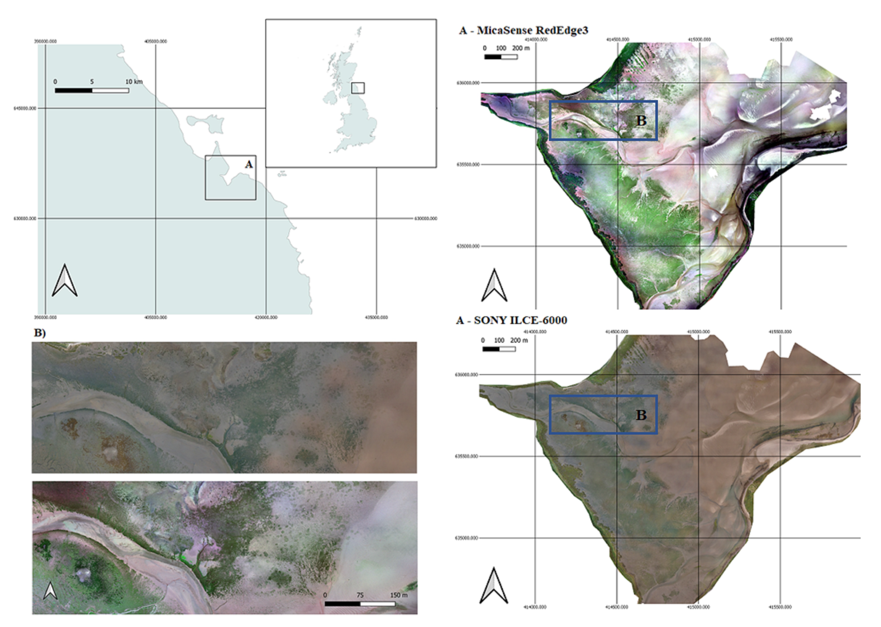
Figure 1 displays very high resolution orthomosaics of Budle Bay created using Agisoft’s MetaShape [57] and structure from motion (SfM). SfM techniques rely on estimating intrinsic and extrinsic camera parameters from overlapping imagery [58]. A combination of appropriate flight planning in terms of altitude and aircraft speed, and the camera’s field of view were important for producing good quality orthomosaics. Two sensors were used—a SONY ILCE-6000 camera with 3 wide banded filters for Red, Green and Blue channels and a ground sampling distance of approximately 3 cm (Figure 1, bottom right). A MicaSense RedEdge3 camera with 5 narrow banded filters for Red (655–680 nms), Green (540–580 nms), Blue (459–490 nms), Red Edge (705–730 nms) and Near Infra-red (800–880 nms) channels and a ground sampling distance of approximately 8 cm (Figure 1, top right).
Each orthomosaic was orthorectified using respective GPS logs of camera positions and ground markers that were spread out across the site. This process ensures that both mosaics were well aligned with respect to each other, and also with ecological features present within the coastal site.
2.3. On-Situ Survey
CEFAS and the Environment Agency conducted ground and aerial surveys of Budle Bay in September 2017 and noted 13 ecological targets that can be grouped into background sediment, algae, seagrass and saltmarsh. Classes within the background sediment were rock, gravel, mud and wet sand. These features were modelled as one single class and dry sand was added to further aid distinguishing sediment features. Algal classes included Microphytobenthos, Enteromorpha spp. and other macroalgae (inc. Fucus). Lastly, the remaining coastal vegetation classes were seagrass and saltmarsh. Since the aim is to map the areas of seagrass in general, both species Zostera noltii and Angustifolia were merged to a single class while saltmarsh remains as a single class although two different species were noted. Thus, a total of seven target classes can be listed.
- Background sediment: dry sand and other bareground
- Algae: Microphytobenthos, Enteromorpha and other macroalgae (including Fucus)
- Seagrass: Zostera noltii and Angustifolia merged to a single class
- Other plants: Saltmarsh
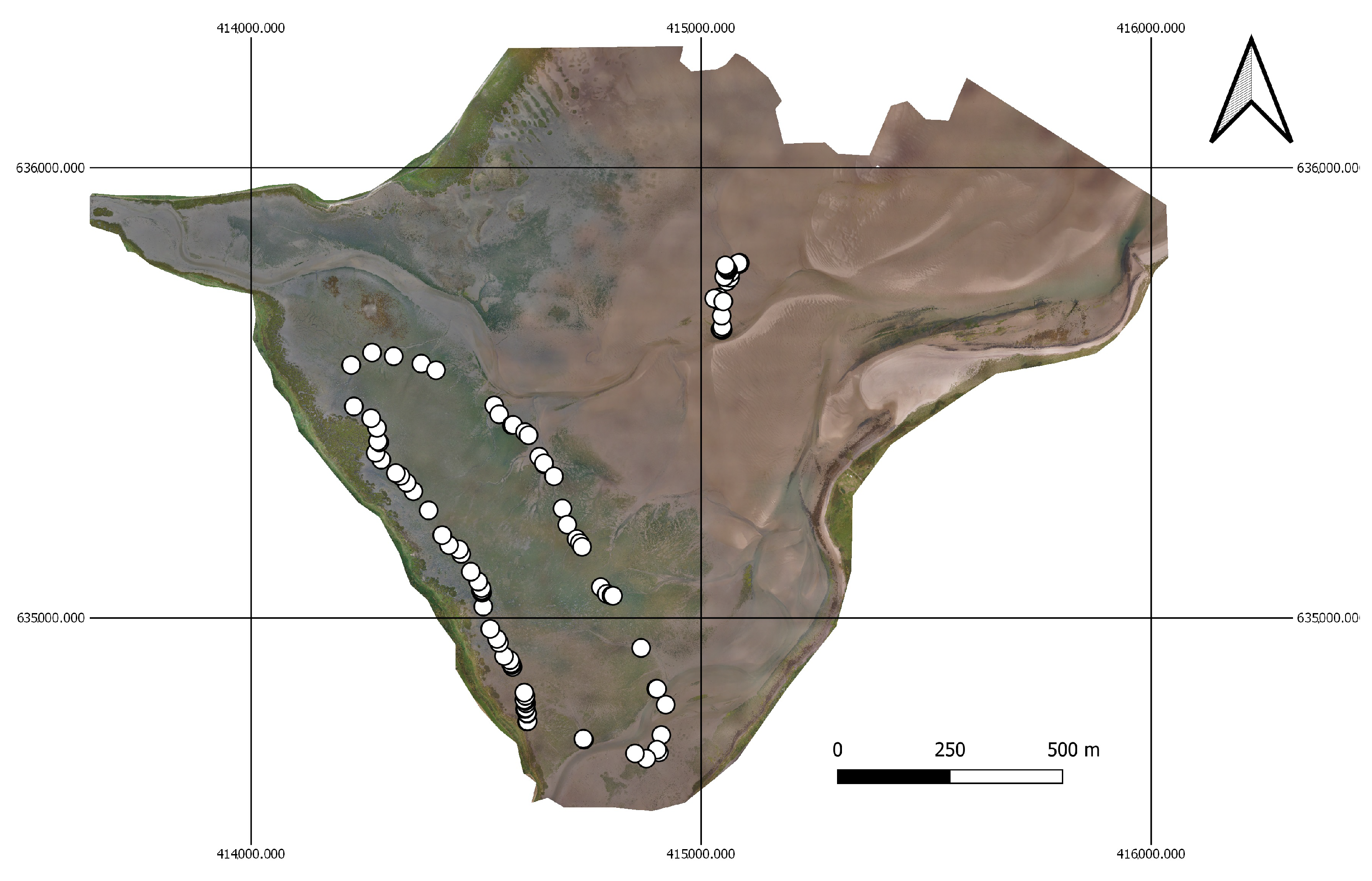
The in-situ survey recorded 108 geographically referenced tags with the percentage cover of all ecological features previously listed within a 300 mm radius. These were dispersed mainly on the Western, Central and Southern portions of the site. Figure 2 displays the spatial distribution of recorded measurements by placing a point for each tag over the orthophoto generated using the SONY camera.
2.4. Data Pre-Processing for FCNNs
The orthomosaic from the SONY camera was 87,730 × 72,328 pixels with 3 image bands orthomosaic, while the RedEdge3 multispectral orthomosaic was 32,647 × 26,534 with 5 image bands. For ease of processing, each orthomosaic was split into non-overlapping blocks of 6000 × 6000 images with each image containing geographic information to be used for further processing. The SONY orthomosaic was split into 140 tiles and the RedEdge3 into 24.
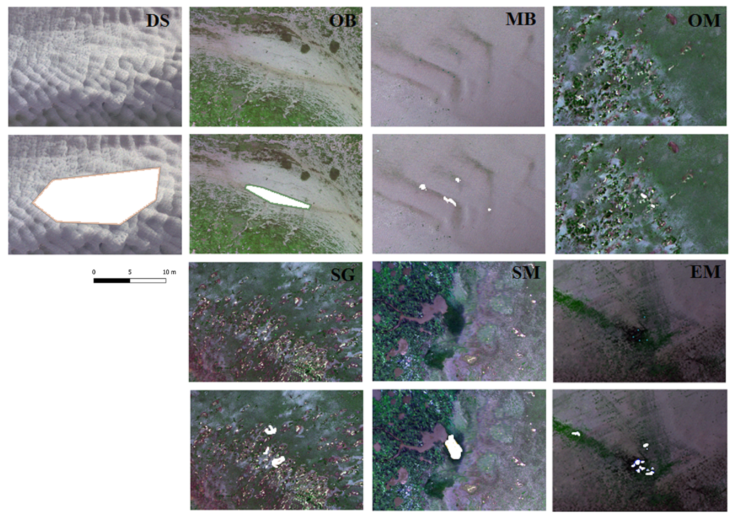
The recorded percentage covers were used to classify each point in Figure 2 to a single ecological class listed in Section 2.3 based on the highest estimated cover during the in-situ survey. The classification for each point provides the basis to create geographically referenced polygon files through photo interpretation. This process generated a total of 56 polygons that were split into train and test sets. The train set had 42 polygons and the test set 14. The reasoning for using photo interpretation instead of selecting segmented image-objects was to avoid bias from the OBIA when generating segmentation maps used for FCNN training. Figure 3 displays a gallery of images for each class with some example polygons.
2.4.1. Polygons to Segmentation Masks for FCNNs
Each polygon contains a unique semantic value depending on the recorded class. FCNNs were trained with segmentation maps that contain a one-to-one mapping of pixels encoded with a semantic value, with the goal to optimise this mapping [47]. Segmentation maps used for training FCNNs were created using the geographic coordinates stored in each polygon and converting real-world coordinates for each vertex to image-coordinates. If a polygon fits within an image, then the candidate image was sampled into 256 × 256 image tiles centered on labelled sections of the image. By cropping images centered on polygons the edges of each image have a number of pixels that were not labelled. The difference in spatial resolution for each camera results in a difference in labelled pixels, since each polygon covers the same area within the real-world. This process generated 534 images with the RedEdge3 multispectral camera from both sets of polygons. Polygons from the train set were split into 363 images for training and 69 images for validation, while test set polygons generated 102 images. The SONY camera produced 1108 images from both sets of polygons. The train set was split into 770 images for training and 125 for validation and the test set of polygons generated 213 images.
2.4.2. Vegetation, Soil and Atmospheric Indices for FCNNs
Vegetation, soil and atmospheric indices are derivations from standard Red, Green and Blue and/or Near-infrared image bands that can aid discerning multiple vegetation classes [59]. Near-infrared, red, green and blue bands from the RedEdge3 were used to compute a variety of indices, adding five bands of data to each input image. These extra bands were: Normalised Difference Vegetation Index (NDVI) [60], Atmospheric Resistant Vegetation Index (IAVI) [61], Modified Soil Adjusted Vegetation Index (MSAVI) [62], Modified Chlorophyll Absorption Ratio Index (MCARI) [63] and Green Normalised Difference Vegetation Index (GNDVI) [64]. The red, green and blue channels for both cameras were used to compute additional four indices, namely Visible Atmospherically Resistant Index (VARI) [65], Visible-band Difference Vegetation Index (VDVI) [66], Normalised Green-Blue Difference Vegetation Index (NGBDI) [67] and Normalised Green-Red Difference Vegetation Index (NGRDI) [68]. The choice of these indices was mostly due to the importance of the green channel for measuring reflected vegetation spectra, while also providing more data for FCNNs to start with before modelling complex one-to-one mappings for each pixel.
The above index images were stacked along the third dimension onto each image resulting in images for the RedEdge3 and the Sony camera having 14 and 7 bands respectively. Furthermore, each individual image band was scaled to a value between 0 and 1.
2.5. Fully Convolutional Neural Networks
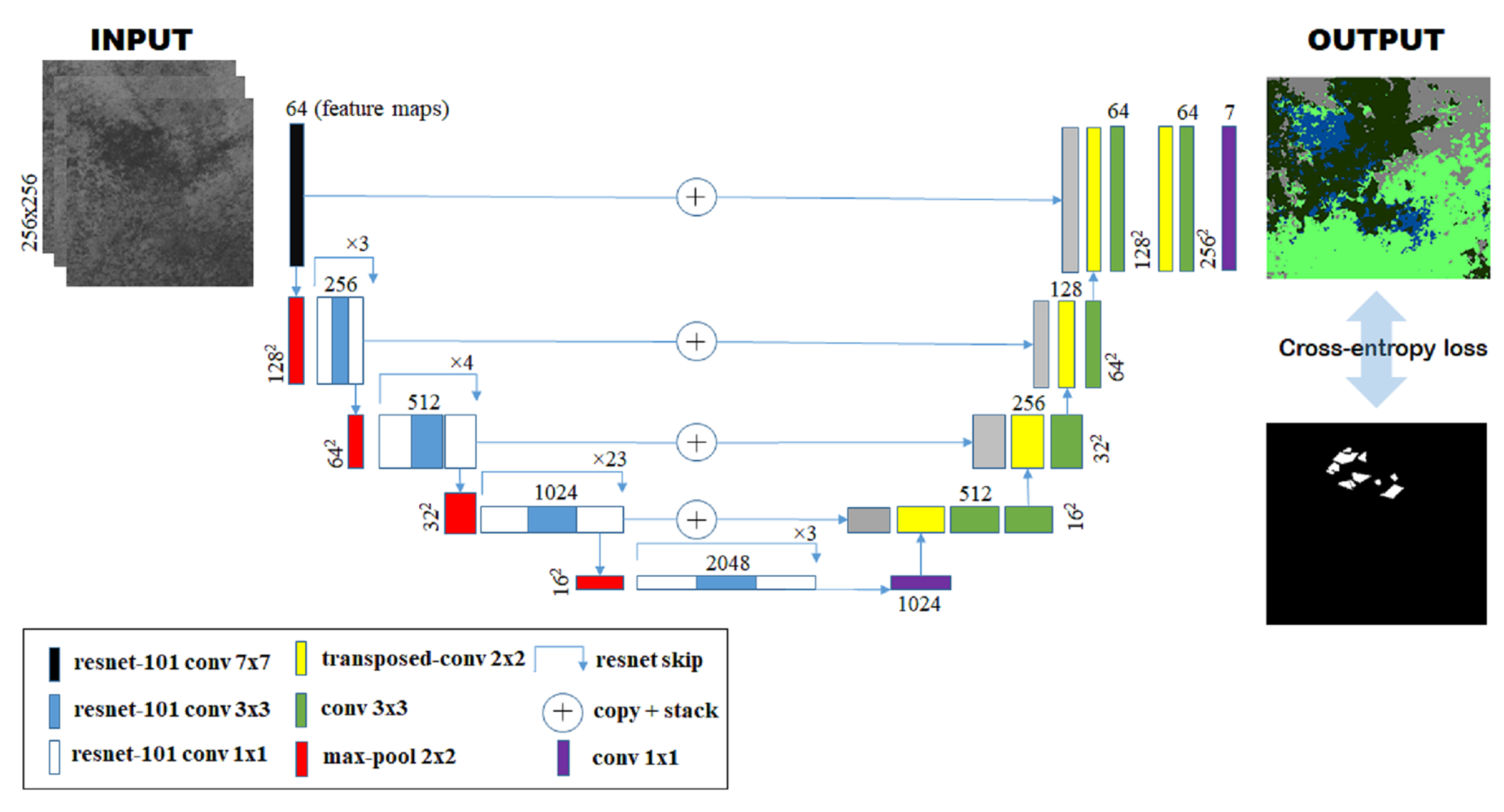
Fully Convolutional Neural Networks [38,47,69] are an extension of traditional CNN architectures [36,70] adapted for semantic segmentation. CNNs usually comprise a series of layers that process lower layer inputs through repeating convolution and pooling operations followed by a final classification layer/s. Each convolution and pooling layer transforms the input image into higher level abstracted representations. FCNNs can be broken down into two networks: an encoder and a decoder network. The encoder network is identical to a CNN, except the final classification layer which is removed. The decoder network applies alternate upsample and convolution operations on feature maps created by the encoder network and a final classification layer with convolution kernels and a softmax function. Network weights and biases are adjusted through gradient descent by minimising the loss function between network outputs and the ground truth pixel labels.
Figure 4 displays the architecture used for this work. The overall architecture is a U-Net [38] and the encoder network is a ResNet101 [71] pre-trained on ImageNet. Residual learning has proven to surpass very deep neural networks [71] and is a suitable encoder network for the overall U-Net architecture. The decoder network applies a transposed convolution for upsampling while also concatenating feature maps from the encoding stage at appropriate resolutions followed by a final convolution. The final convolution condenses feature maps to have the same number of channels as the total number of classes before a softmax transfer function classifies each pixel.
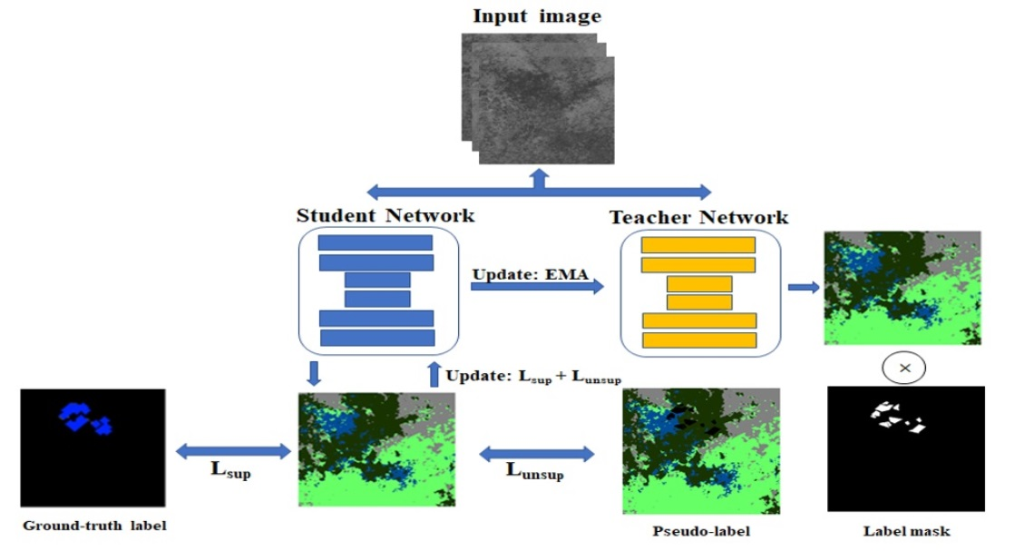
For semi-supervised training the Teacher-Student method was used [48]. This approach requires two networks: a teacher and a student, both having the same architecture as shown in Figure 4. The student network is updated through gradient descent minimising the sum of two loss terms: a supervised loss calculated on labelled pixels of each segmentation map, and conversely, an unsupervised loss calculated using non-labelled pixels. The teacher network is updated using an exponential moving average of weights from the student network.
2.5.1. Weighted Training for FCNNs
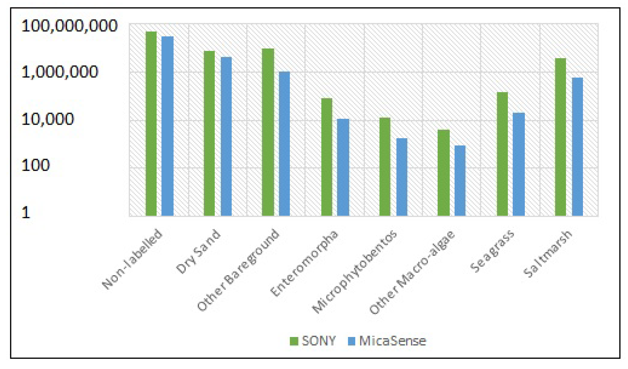
Section 2.4 detailed the process of creating segmentation maps from polygons. Both sets of images from each camera had an imbalanced target class distribution. Figure 5 shows the number of labelled pixels per class and also the number of non-labelled pixels for each camera.
The recorded distribution poses a challenge for classes such as other macroalgae and Microphytobentos due to the relative number of labelled pixels in comparison with the remaining target classes. The pixel counts shown in Figure 5 were used to calculate the probability of each class occurring within the training set, and for each class a weight was calculated by taking the inverse for each probability. During FCNN training the supervised loss was scaled with respect to these weights.
where, is weight for a given class probability and K is the total number of classes.
2.5.2. Supervised Loss
For the supervised loss term, consider and to be respectively, a mini-batch of images and corresponding segmentation maps; where B, C, H and W are respectively, batch size, number of input channels, height and width. Processing a mini-batch with the student network outputs per-pixel scores ; where K is the number of target classes. The softmax transfer function converts network scores into probabilities by normalising all K scores for each pixel to sum to one.
where, ; is a pixel location and is the probability for the channel at pixel location x, with . The negative log-likelihood loss is calculated between segmentation maps and network probabilities.
For each image, the supervised loss is the sum of all losses for each pixel using Equation (3) and averaged according to the number of labelled pixels within Y.
2.5.3. Unsupervised Loss
Previous work in semi-supervised segmentation details using a Teacher-Student model and advanced data augmentation methods in order to create two images for each network to process [49,50]. While this work did not use data augmentation methods, pairs of images were created using labelled and non-labelled pixels within Y.
Similarly to the supervised loss term, a mini-batch of images is passed through both the student and the teacher networks, producing per-pixel scores and respectively. Again, pixel scores are converted to probabilities with softmax (Equation (2)), respectively producing and for the two networks. The maximum-likelihood of teacher predictions was used to create pseudo segmentation maps to compute the loss for non-labelled pixels of Y. Thus, the unsupervised loss is also calculated similarly to Equation (3) but the negative log-likelihood is computed between predictions from the student model () and a pseudo map () of pixels that are initially non-labelled.
For each image, the unsupervised loss was the sum of all losses for each pixel using Equation (4) averaged according to the number of non-labelled pixels within Y. The latter loss was also scaled with respect to the confidence in predictions for the teacher network so that initial optimisation steps focus more on the supervised loss term. Classes with low labelled pixel count would benefit from the unsupervised loss term, as confident teacher predictions can guide the decision boundaries of student models by adding pseudo maps to consider.
2.5.4. Training Parameters
Combining both loss terms yields the objective cost used for optimising FCNNs in a semi-supervised setting.
where and are respectively the supervised and unsupervised loss term. The supervised loss was scaled according to the weights computed in Equation (1) and the unsupervised loss to which was set to 0.1 for all experiments.
All networks were pre-trained on ImageNet. Networks for each camera were trained for 150 epochs with a batch-size of 16 using Adam optimiser. The learning rate was initially set to 0.001 and reduced by a factor of 10 every 70 epochs of training. All FCNNs were implemented and trained using Pytorch version 10.2.
2.6. OBIA
The OBIA method for modelling multiple coastal features was performed using eCognition v9.3 [72]. This software has the tools to process high resolution orthomosaics and shape file exports from GISs to create supervised models. Section 2.4 detailed a number of methods used to pre-process the orthomosaics and shape polygons, however the OBIA does not require this.
The first step in OBIA is to process each orthomosaic using a multiresolution segmentation algorithm to partition the image into segments, also known as image-objects [72]. The segmentation starts with individual pixels and clusters pixels to image-objects using one or more criteria of homogeneity. The subsequent clustering of two adjacent image-objects or image-objects that are a subset of each other are merged together based one the following criterion:
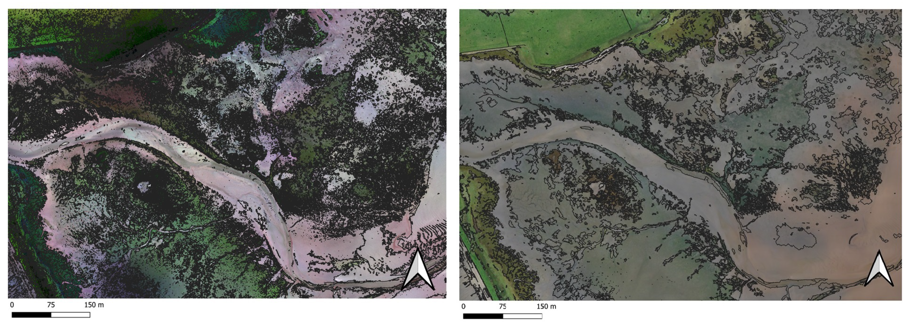
where , and respectively represent the pixel values for objects 1, 2 and a candidate virtual merge m. N and M are the number of total pixels, respectively for objects 1 and 2. This criterion evaluates the change in homogeneity during fusion of image-objects. If this change exceeds a certain threshold value, then the fusion is not performed. In contrast, if the change in image-objects is below the threshold, then both candidates are clustered to form a larger region. The segmentation procedure stops when no further fusions are possible without exceeding the threshold value. In eCognition, this threshold value is a hyper-parameter defined at the start of the process and is also known as the scale parameter. The geometry of each shape is defined by two other hyper-parameters—shape and compactness. For this work, the scale parameter was set to 200, the shape to 0.1 and the compactness to 0.5. Figure 6 shows image objects overlaid on top of both orthomosaics.
In Section 2.4.1, the split of polygons used for training and testing has been detailed. Each polygon (Figure 3) from the training set was overlaid on top of image-objects to select the candidate segments for extracting spectral features. Selected image-objects create a database for the in-built Random Forest [73] in eCognition. The spectral features for the RedEdge3 camera were channel mean and standard deviation, vegetation and soil indices (NDVI, RVI, GNDVI, SAVI), ratios between red/blue, red/green and blue/green image layers and the intensity and saturation components of the HSI colour space. The features for the SONY were the same, but the vegetation and soil indices were not added. Once the features and image-objects were selected, the Random Forest modeller produced a number of Decision Trees [74] with each tree being optimised on features using the GINI Index.
2.7. Accuracy Assessment
The measurements used to objectively quantify results were pixel accuracy, precision, recall and F1-score. Pixel accuracy was the ratio between pixels that were classified correctly and the total number of labelled pixels within the test set for a given class. Precision and recall are metrics that can show how a classifier performs for each specific class. F1-score is the harmonic mean of recall and precision and is therefore a suitable metric to quantify classifier performance when a single figure of merit is needed. Equation (7) details each of these metrics where , , and were respectively, True Positive, True Negative, False Positive and False Negative pixel classifications.
3. Results
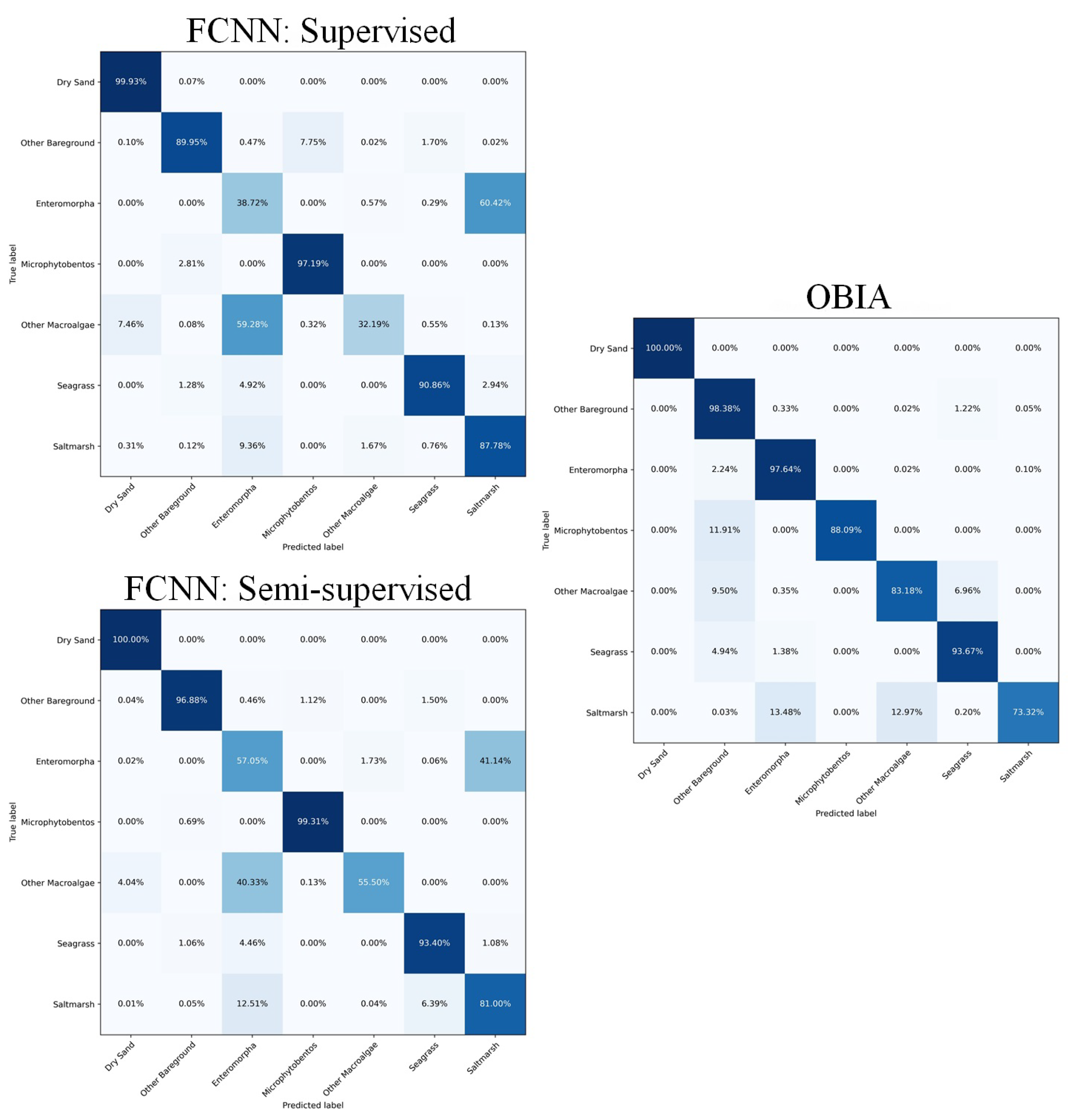
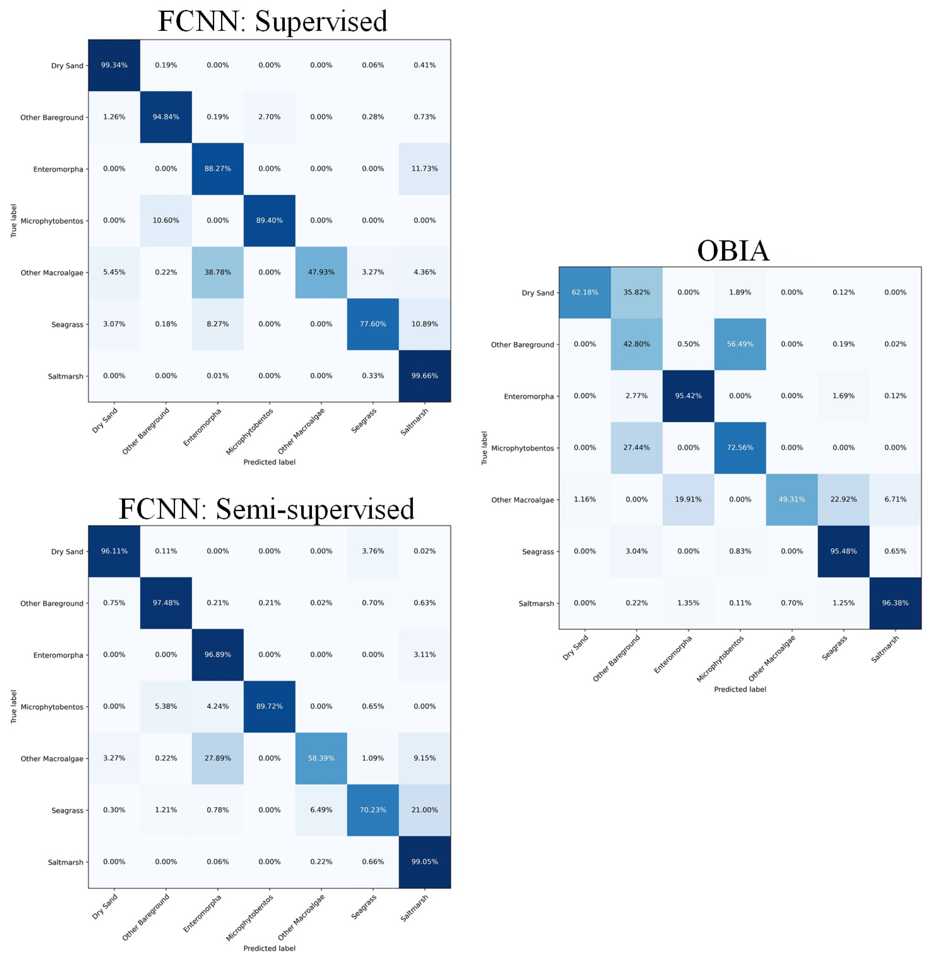
The outputs for both the FCNNs and OBIA were compared with a subset of polygons that were not used for training. Figure 7 and Figure 8 display confusion matrices scoring outputs from each method and camera as pixel accuracy. The confusion matrices also show pixel accuracies for FCNN models that were optimised using only Equation (3) and models that were optimised using both Equations (3) and (4). The confusion matrices reflect average results over three training runs with the set of hyper-parameters described in Section 2.5.4. Overall results for OBIA and FCNNs in a semi-supervised setting for each camera can be viewed in Table 1, where precision, recall and F1-score are reported. Figure 9 displays habitat maps for each method and camera.
3.1. SONY ILCE-6000 Results
Predictions with the OBIA method had an average pixel accuracy of 90.6%. Classes related to sediment had scores of 100% and 98.38%, respectively for dry sand and other bareground. Algal classes scored 97.6%, 88.09% and 83.18%, respectively for Enteromorpha, Microphytobentos and other macroalgae (inc. Fucus). Seagrass predictions were found to score 93.67% and saltmarsh was the worst performing class for the OBIA with 73.32%.
FCNNs yielded an average class accuracy of 76.79% and 83.3%, respectively for supervised and semi-supervised settings. Both approaches scored close to 100% for dry sand and other bareground performed better in a semi-supervised setting scoring 96.88%. Scores for Enteromorpha and other macroalgae (inc. Fucus) were respectively 38.72% and 32.29% for supervised training and 57.05% and 55.90% for semi-supervised training. Seagrass scored similarly in both training settings with approximately 90% and saltmarsh scored better in a supervised setting with 87.78%, while the semi-supervised setting scored 81%.
3.2. MicaSense RedEdge3 Results
The OBIA method had an average pixel accuracy of 73.44%. Sediment classes such as dry sand and other bareground scored 63.18% and 42.80%. Algal classes scored 93.42%, 72.54% and 49.31%, respectively for Enteromorpha, Microphytobentos and other macroalgae (inc. Fucus). The remaining vegetation classes of seagrass and saltmarsh both presented high scores of 95.48% and 96.38.
FCNNs yielded an average class accuracy of 85.27% and 88.44%, respectively for supervised and semi-supervised settings. Both models had good scores for sediment classes scoring above 95% in pixel accuracy. Algal classes of Enteromorpha, Microphytobentos and other macroalgae (inc. Fucus) respectively scored for supervised and semi-supervised training (88.22%, 96.29%), (89.40%, 89.72%) and (47.93%, 58.39%). Seagrass predictions scored 77.68% and 70.23 respectively for supervised and semi-supervised training, while saltmarsh was found to score 99% in both settings.
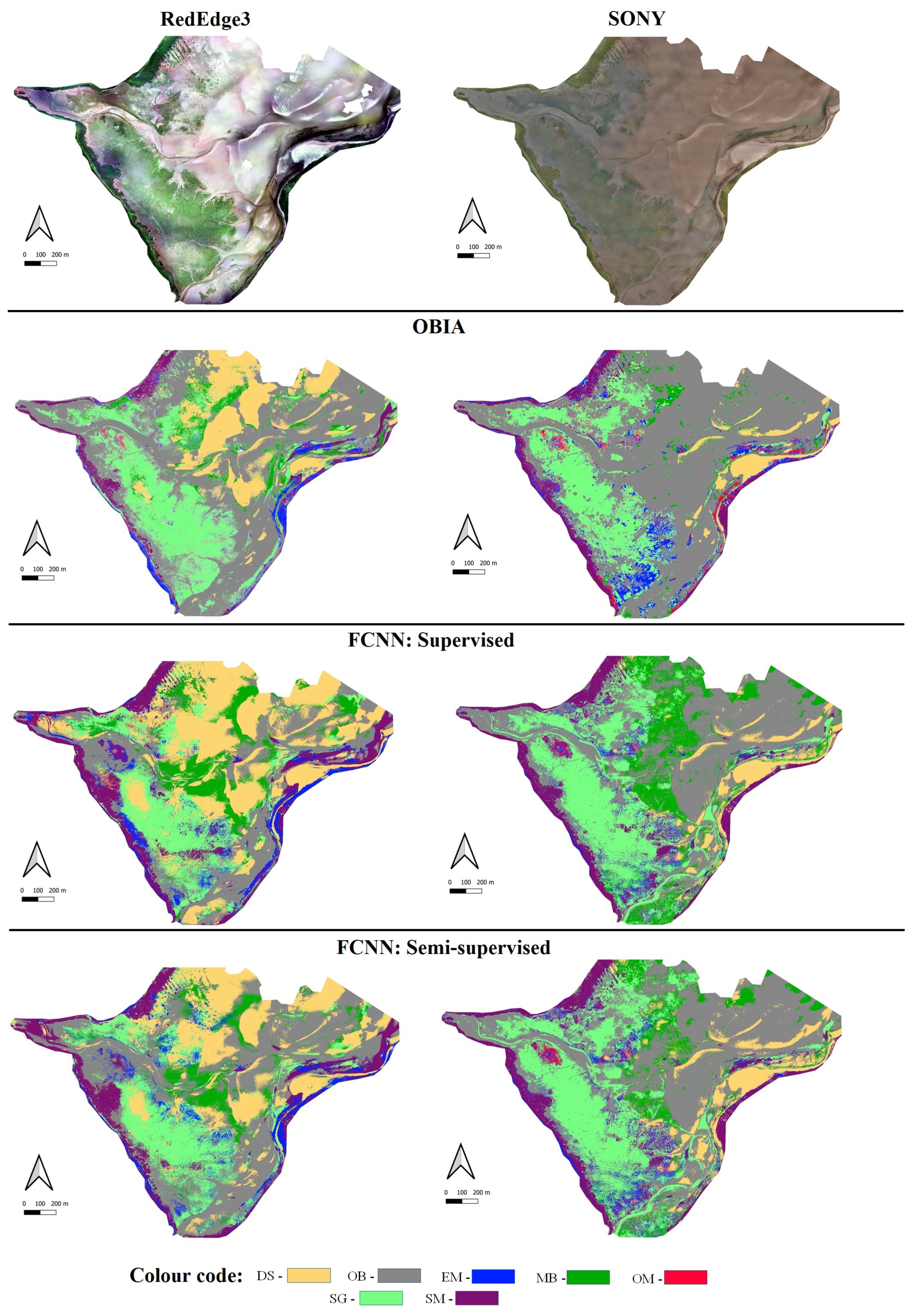
3.3. Habitat Maps
Figure 9 shows the habitat maps of Budle Bay for each camera and method previously described.
4. Discussion
Figure 7, Figure 8 and Figure 9 as well as Table 1 indicate that FCNNs provide comparable performance to OBIA. Figure 7 and Figure 8 also show an increase in performance for the semi-supervised FCNN models in comparison to the fully-supervised.
4.1. FCNNs Convergence
The convergence of FCNNs was analysed by testing multiple settings for learning rate and assessing computed confusion matrices as well as training and validation losses over several runs of the algorithm. This ensured that all models converged appropriately. Figure 7 and Figure 8 show average pixel accuracy scores over three sequential runs with the same hyper-parameters described in Section 2.5.4.
4.2. SONY ILCE-6000 Analysis
Habitat maps from the SONY camera were found to perform better with the OBIA than FCNNs in terms of average pixel accuracy and F1-score. Respectively, the OBIA had an average accuracy and F1-score of 90.6% and 0.71, while FCNNs in a semi-supervised setting had 83.3% and 0.65.
Sediment class predictions for both methods scored well, with both metrics either scoring above 90% or above 0.9, respectively for pixel accuracy and F1-score. This suggests that the OBIA and FCNNs methods successfully predicted test polygons for sediment classes while also avoiding false positive and false negative pixel classifications.
Algal classes were found to have mixed performance depending on the method used. Scores in Figure 7 with OBIA noted that classes of Enteromorpha and other macroalgae (inc. Fucus) scored better, while Microphytobentos were more accurate with FCNNs. However, scores in Table 1 for the same classes suggest that OBIA performed better for classes of Enteromorpha and Microphytobentos, while FCNNs scored better for other macroalgae. Analysing areas in Figure 9 that were predicted as Enteromoprha with OBIA and comparing these areas with FCNN habitat maps show that the latter method interchangeably predicts Enteromorpha and saltmarsh. This observation can be supported by Figure 7 where 60.43% and 41.14% of test labels for Enteromorpha were predicted as saltmarsh, respectively for supervised and semi-supervised settings. These points suggest that habitat maps detailing areas for Enteromorpha with OBIA were more likely to be correct. Pixel classifications in Figure 3 for Microphytobentos indicate that FCNNs performed well and accurately mapped test polygons of Microphytobentos, however figures for precision and F1 in Table 1 also indicate that FCNNs have high false positive rate for this class. Conversely, OBIA produced a perfect figure for precision which indicates that no pixel classifications for test polygons were false positive. This high false positive rate for Microphytobentos can be noticed by comparing the areas mapped as other bareground using OBIA that were mapped as Microphytobentos for FCNNs. Therefore, habitat maps with OBIA were more likely to be correct for predictions of Microphytobentos. Other macroalgae (ic. Fucus) was found to be a problematic class for FCNNs due to the low number of labelled pixels relative to the rest of the dataset (Figure 5). Confusion matrices in Figure 7 show that other macroalgae were often classified as Enteromorpha, which is another algae present in Budle Bay. However, they also show that the semi-supervised results were much better than the results in the supervised setting, which supports the premise in Section 2.5.3 that an unsupervised loss term on pseudo segmentation maps could help datasets with a relative low number of labelled pixels. While scores show that OBIA performs better on classification of other macroalgae, Table 1 shows that the F1-score was lower with OBIA than FCNNs, which was mainly due to the OBIA low precision score. Habitat maps in Figure 9 show that most areas classified as other macroalgae are similar for both approaches.
The confusion matrix also shows that scores for seagrass are high for both methods. However, Table 1 also shows that precision figures were 0.64 and 0.27, respectively for OBIA and FCNNs. This again suggests a high false positive rate for FCNNs, with habitat maps in Figure 9 also detailing more areas mapped as seagrass with FCNNs than with OBIA. Therefore, areas mapped as seagrass with OBIA were more likely to be correct than FCNNs. The results for saltmarsh were in general very similar for both methods. Scores in the confusion matrix show that saltmarsh polygons was 73.32% for OBIA, and 87.78% and 81.0% for FCNNs, respectively for supervised and semi-supervised settings. The F1-score was 0.84 and 0.88, respectively for OBIA and FCNNs. This suggests that OBIA was more likely to classify pixels within saltmarsh polygons incorrectly, although overall both maps present similar areas mapped as saltmarsh.
4.3. MicaSense RedEdge3 Analysis
Habitat maps from the RedEdge3 multispectral camera were found to be more correct with the FCNNs than OBIA in terms of both average pixel accuracy and F1-score. The OBIA had an average accuracy and F1-score of 73.4% and 0.60, while semi-supervised FCNN had 88.44% and 0.78. In terms of both pixel accuracy and F1-score for sediment classes, FCNNs were found to perform better than OBIA. The confusion matrix for the latter method in Figure 8 shows that 35.82% of pixels in dry sand polygons were classified as other bareground, while Table 1 shows figures of 0.99 for precision and 0.62 for recall. This would suggest that false negative classifications for dry sand were mostly other bareground. Figure 8 shows FCNNs in both settings achieved scores of 98% matrix and the semi-supervised setting had an F1-score of 0.98, which suggests that FCNNs accurately mapped dry sand test polygons. However, the habitat maps in Figure 9 note some differences in areas mapped as dry sand for each method. In particular, supervised FCNNs were found to classify larger areas as dry sand, whereas semi-supervised FCNNs produced similar results to OBIA. OBIA classified 56.49% of other bareground polygon pixels as Microphytobentos. In Section 2.3, other bareground was noted to include wet sand, while Microphytobentos is a unicellular eukaryotic algae and cyanobacteria that grow within the upper millimeters of illuminated sediments, typically appearing only as a subtle greenish shading [75]. This could provide some reasoning for other bareground and Microphytobentos being interchangeably classified with one another with OBIA. Similarly to dry sand, FCNNs performed well in terms of both pixel accuracy and F1-score which suggest that other bareground polygons were classified correctly without producing many false positives.
Figure 8 and Table 1 show the scores for algal classes were higher with FCNNs than with OBIA. However, both methods were in fact similar in terms of these figures, with the exception of F1-score for other macroalgae with OBIA. The confusion matrix in Figure 8 shows that both OBIA and FCNN classifications for Microphytobentos exhibited poor precision. Similarly to the SONY camera, this can be noticed by large areas in Figure 9 being predicted as Microphytobentos instead of other bareground, especially for FCNNs in a supervised setting. Both methods mapped Enteromorpha in similar areas, but FCNNs included classifications for Enteromorpha in the center and the south eastern boundary of the site, while OBIA predicted mostly seagrass and other bareground for the same stated areas. Other macroalgae class was found to have better results with FCNNs over OBIA. Moreover, comparing supervised and semi-supervised models, we note an increase in performance when the unsupervised loss term was added to the training algorithm, which supports the initial hypothesis that the unsupervised loss term aids FCNNs with target classes that have a low number of labelled pixels relative to the remaining classes.
The remaining vegetation classes of seagrass and saltmarsh were found to have good performance with both methods, however the OBIA was found to perform better with respect to seagrass classifications. Both Figure 8 and Table 1 supported this with recall scores being lower with FCNNs than OBIA. As mentioned, low recall indicates high false negative rate and interestingly all FCNNs did not predict seagrass along the north western part of the site (area covered in Figure 6). While it is not possible to quantify which method was correct without surveying the site again, the confidence in seagrass predictions for OBIA along with FCNNs predicting bareground sediment instead of vegetation can lead to users being more confident with OBIA for seagrass mapping. Both methods performed same for saltmarsh and habitat maps in Figure 9 show that most predicted areas were similar, however FCNNs were found to interchangeably classify saltmarsh and seagrass which is also supported by Figure 8, where each confusion matrix for FCNNs predicted a number of seagrass test polygon pixels as saltmarsh.
4.4. Overall Analysis
In the discussion of the results for both cameras we have found two key results.
The first result is that OBIA continues to be a suitable method for intertidal seagrass mapping while assessing multiple coastal features of algae and sediment within a site. Figure 7 and Figure 8 as well as Table 1 reported pixel accuracy and F1-score that would suggest some degree of confidence for areas classified as seagrass with OBIA within the maps shown in Figure 9. A plethora of other studies have mapped intertidal seagrass using OBIA with encouraging results [16,19,76,77]. However, this work also attempted to make a direct comparison between FCNNs and OBIA and showed that the latter outperformed the proposed method with respects to intertidal seagrass mapping. Furthermore, the provided analysis recorded accuracies for supervised classifications at a pixel-level. Some work on intertidal seagrass mapping give confusion matrices for supervised classification where accuracies reflect the percentage of segmented image-objects through MRS that were classified correctly [19] and geographically referenced shape points [77]. The work in [76] also performed an analysis of OBIA for intertidal seagrass mapping at a pixel-level, however this work also considered mapping intertidal seagrass at various density levels, which adds complexity to the mapping task. In fact, seagrass mapping can also be considered as a regression problem instead of classification [16,78]. Other work using FCNNs for seagrass mapping was found in [79,80,81]. However, these studies were mainly concerned with subtidal seagrass meadows instead of intertidal seagrass. FCNNs have been used for mapping intertidal macroalgae [82] with reported average accuracies for a 5 class problem to be 91.19%. Yet, this work considered mapping intertidal macroalgae, seagrass and sediment features at a coarser resolution. In fact, this was to the authors’ knowledge the first use of FCNNs for intertidal seagrass mapping.
The second key result is that although FCNNs performed worse for seagrass mapping, overall results shown in Section 3 noted that FCNNs had a comparable performance with OBIA in terms of average pixel accuracy and F1-score. Moreover, Figure 7 and Figure 8 as well as habitat maps in Figure 9 showed that a semi-supervised setting could increase the overall performance of FCNNs, reducing the need for more labelled data. This was particularly true for other macroalage (inc. Fucus) which benefited the most from a semi-supervised training mode. Recent applications for semi-supervised segmentation have shown to produce state of the art results with subsets of labelled data [49,50,83,84], which can provide alternate modelling approaches for FCNNs in practical applications where labelled data is limited. Studies within remote sensing often have very limited amounts of labelled data while the recent trends show the use of weakly-supervised and semi-supervised training regimes may be utilised to overcome this problem [85,86,87]. In particular, [87] applies adversarial training for seagrass mapping to overcome the domain shift from mapping in different coastal environments, while this work leverages non-labelled parts of each image to produce pseudo-labels in a Teacher-Student framework.
5. Conclusions
In this work, we showed that FCNNs trained from a small set of polygons can be used for segmentation of intertidal habitat maps in high resolution aerial imagery. Each FCNN was evaluated in two training modes, supervised and semi-supervised, with results indicating that semi-supervision helps with segmentation of target classes that have a small number of labelled pixels. This prospect may be of benefit in studies where in-situ surveying is an expensive effort to conduct.
We also showed that OBIA continues to be a robust approach for monitoring multiple coastal features in high resolution imagery. In particular, OBIA was found to be more accurate than FCNNs in predicting seagrass for both cameras. However, as noted in Section 3 OBIA results were highly dependant on the initial parameters used for MRS, with the scale parameter being critical for image-object creation.
The study site and problem formation described in Section 2.3 combined for a complex problem. This in turn can make confidence in seagrass predictions decrease as ambiguity over multiple vegetation classes increases. OBIA was found to overcome this for both cameras accurately predicting seagrass polygons while maintaining relatively high precision when compared to FCNNs. On the other hand, FCNNs were found to be more accurate in classifying algal classes, in particular other macroalgae, which had the least number of labelled pixels. Therefore, while this work shows that OBIA is a suitable method for intertidal seagrass mapping, other applications within remote sensing for coastal monitoring with restricted access to in-situ data can utilise semi-supervised FCNNs.
Author Contributions
Conceptualization, B.H., M.M., J.B., T.D.; methodology, B.H., R.A., G.F.; software, B.H., R.A., G.F.; data curation, B.H., J.B., T.D.; writing—original draft preparation, B.H.; writing—review and editing, B.H., M.M., J.B., T.D., R.A.; All authors have read and agreed to the published version of the manuscript.
Funding
This research was funded by Cefas, Cefas Technology and the Natural Environmental Research Council through the NEXUSS CDT, grant number NE/RO12156/1, titled “Blue eyes: New tools for monitoring coastal environments using remotely piloted aircraft and machine learning”.
Data Availability Statement
All source code for model architecture, training and loss computation is publicly available at https://github.com/BrandonUEA/Budle-Bay. The data presented in this study are available on request from the corresponding author. The data are not publicly available due to crown copyright.
Acknowledgments
The authors thank Cefas and the EA for providing necessary imagery as well as data from the in-situ survey used to generated shape polygons.
Conflicts of Interest
The authors declare no conflict of interest.
Abbreviations
The following abbreviations are used in this manuscript:
| RS | Remote Sensing |
| FCNN | Fully Convolutional Neural Network |
| MRS | Multi-Resolution Segmentation |
| OBIA | Object-Based Image Analysis |
References
- Fonseca, M.S.; Zieman, J.C.; Thayer, G.W.; Fisher, J.S. The role of current velocity in structuring eelgrass (Zostera marina L.) meadows. Estuar. Coast. Shelf Sci. 1983, 17, 367–380. [Google Scholar] [CrossRef]
- Fonseca, M.S.; Bell, S.S. Influence of physical setting on seagrass landscapes near Beaufort, North Carolina, USA. Mar. Ecol. Prog. Ser. 1998, 171, 109–121. [Google Scholar] [CrossRef] [Green Version]
- Gera, A.; Pagès, J.F.; Romero, J.; Alcoverro, T. Combined effects of fragmentation and herbivory on Posidonia oceanica seagrass ecosystems. J. Ecol. 2013, 101, 1053–1061. [Google Scholar] [CrossRef] [Green Version]
- Pu, R.; Bell, S.; Meyer, C. Mapping and assessing seagrass bed changes in Central Florida’s west coast using multitemporal Landsat TM imagery. Estuar. Coast. Shelf Sci. 2014, 149, 68–79. [Google Scholar] [CrossRef]
- Short, F.T.; Wyllie-Echeverria, S. Natural and human-induced disturbance of seagrasses. Environ. Conserv. 1996, 23, 17–27. [Google Scholar] [CrossRef]
- Marbà, N.; Duarte, C.M. Mediterranean warming triggers seagrass (Posidonia oceanica) shoot mortality. Glob. Chang. Biol. 2010, 16, 2366–2375. [Google Scholar] [CrossRef]
- Duarte, C.M. The future of seagrass meadows. Environ. Conserv. 2002, 29, 192–206. [Google Scholar] [CrossRef] [Green Version]
- McGlathery, K.J.; Reynolds, L.K.; Cole, L.W.; Orth, R.J.; Marion, S.R.; Schwarzschild, A. Recovery trajectories during state change from bare sediment to eelgrass dominance. Mar. Ecol. Prog. Ser. 2012, 448, 209–221. [Google Scholar] [CrossRef] [Green Version]
- Lamb, J.B.; Van De Water, J.A.; Bourne, D.G.; Altier, C.; Hein, M.Y.; Fiorenza, E.A.; Abu, N.; Jompa, J.; Harvell, C.D. Seagrass ecosystems reduce exposure to bacterial pathogens of humans, fishes, and invertebrates. Science 2017, 355, 731–733. [Google Scholar] [CrossRef]
- Fourqurean, J.W.; Duarte, C.M.; Kennedy, H.; Marbà, N.; Holmer, M.; Mateo, M.A.; Apostolaki, E.T.; Kendrick, G.A.; Krause-Jensen, D.; McGlathery, K.J.; et al. Seagrass ecosystems as a globally significant carbon stock. Nat. Geosci. 2012, 5, 505–509. [Google Scholar] [CrossRef]
- Macreadie, P.; Baird, M.; Trevathan-Tackett, S.; Larkum, A.; Ralph, P. Quantifying and modelling the carbon sequestration capacity of seagrass meadows–a critical assessment. Mar. Pollut. Bull. 2014, 83, 430–439. [Google Scholar] [CrossRef]
- Dennison, W.C.; Orth, R.J.; Moore, K.A.; Stevenson, J.C.; Carter, V.; Kollar, S.; Bergstrom, P.W.; Batiuk, R.A. Assessing water quality with submersed aquatic vegetation: Habitat requirements as barometers of Chesapeake Bay health. BioScience 1993, 43, 86–94. [Google Scholar] [CrossRef]
- Waycott, M.; Duarte, C.M.; Carruthers, T.J.; Orth, R.J.; Dennison, W.C.; Olyarnik, S.; Calladine, A.; Fourqurean, J.W.; Heck, K.L.; Hughes, A.R.; et al. Accelerating loss of seagrasses across the globe threatens coastal ecosystems. Proc. Natl. Acad. Sci. USA 2009, 106, 12377–12381. [Google Scholar] [CrossRef] [Green Version]
- Richards, J.A.; Richards, J. Remote Sensing Digital Image Analysis; Springer: Berlin, Germany, 1999; Volume 3. [Google Scholar]
- Anderson, K.; Gaston, K.J. Lightweight unmanned aerial vehicles will revolutionize spatial ecology. Front. Ecol. Environ. 2013, 11, 138–146. [Google Scholar] [CrossRef] [Green Version]
- Duffy, J.P.; Pratt, L.; Anderson, K.; Land, P.E.; Shutler, J.D. Spatial assessment of intertidal seagrass meadows using optical imaging systems and a lightweight drone. Estuar. Coast. Shelf Sci. 2018, 200, 169–180. [Google Scholar] [CrossRef]
- Turner, D.; Lucieer, A.; Watson, C. An automated technique for generating georectified mosaics from ultra-high resolution unmanned aerial vehicle (UAV) imagery, based on structure from motion (SfM) point clouds. Remote Sens. 2012, 4, 1392–1410. [Google Scholar] [CrossRef] [Green Version]
- Collin, A.; Dubois, S.; Ramambason, C.; Etienne, S. Very high-resolution mapping of emerging biogenic reefs using airborne optical imagery and neural network: The honeycomb worm (Sabellaria alveolata) case study. Int. J. Remote Sens. 2018, 39, 5660–5675. [Google Scholar] [CrossRef] [Green Version]
- Ventura, D.; Bonifazi, A.; Gravina, M.F.; Belluscio, A.; Ardizzone, G. Mapping and classification of ecologically sensitive marine habitats using unmanned aerial vehicle (UAV) imagery and object-based image analysis (OBIA). Remote Sens. 2018, 10, 1331. [Google Scholar] [CrossRef] [Green Version]
- Rossiter, T.; Furey, T.; McCarthy, T.; Stengel, D.B. UAV-mounted hyperspectral mapping of intertidal macroalgae. Estuar. Coast. Shelf Sci. 2020, 242, 106789. [Google Scholar] [CrossRef]
- Wilson, B.R.; Brown, C.J.; Sameoto, J.A.; Lacharité, M.; Redden, A.M.; Gazzola, V. Mapping seafloor habitats in the Bay of Fundy to assess megafaunal assemblages associated with Modiolus modiolus beds. Estuar. Coast. Shelf Sci. 2021, 252, 107294. [Google Scholar] [CrossRef]
- Fogarin, S.; Madricardo, F.; Zaggia, L.; Sigovini, M.; Montereale-Gavazzi, G.; Kruss, A.; Lorenzetti, G.; Manfé, G.; Petrizzo, A.; Molinaroli, E.; et al. Tidal inlets in the Anthropocene: Geomorphology and benthic habitats of the Chioggia inlet, Venice Lagoon (Italy). Earth Surf. Process. Landf. 2019, 44, 2297–2315. [Google Scholar] [CrossRef]
- Costa, B.; Battista, T.; Pittman, S. Comparative evaluation of airborne LiDAR and ship-based multibeam SoNAR bathymetry and intensity for mapping coral reef ecosystems. Remote Sens. Environ. 2009, 113, 1082–1100. [Google Scholar] [CrossRef]
- Foody, G.M. Status of land cover classification accuracy assessment. Remote Sens. Environ. 2002, 80, 185–201. [Google Scholar] [CrossRef]
- Blaschke, T. Object based image analysis for remote sensing. ISPRS J. Photogramm. Remote Sens. 2010, 65, 2–16. [Google Scholar] [CrossRef] [Green Version]
- Su, W.; Li, J.; Chen, Y.; Liu, Z.; Zhang, J.; Low, T.M.; Suppiah, I.; Hashim, S.A.M. Textural and local spatial statistics for the object-oriented classification of urban areas using high resolution imagery. Int. J. Remote Sens. 2008, 29, 3105–3117. [Google Scholar] [CrossRef]
- Flanders, D.; Hall-Beyer, M.; Pereverzoff, J. Preliminary evaluation of eCognition object-based software for cut block delineation and feature extraction. Can. J. Remote Sens. 2003, 29, 441–452. [Google Scholar] [CrossRef]
- Butler, J.D.; Purkis, S.J.; Yousif, R.; Al-Shaikh, I.; Warren, C. A high-resolution remotely sensed benthic habitat map of the Qatari coastal zone. Mar. Pollut. Bull. 2020, 160, 111634. [Google Scholar] [CrossRef]
- Husson, E.; Ecke, F.; Reese, H. Comparison of manual mapping and automated object-based image analysis of non-submerged aquatic vegetation from very-high-resolution UAS images. Remote Sens. 2016, 8, 724. [Google Scholar] [CrossRef] [Green Version]
- Purkis, S.J.; Gleason, A.C.; Purkis, C.R.; Dempsey, A.C.; Renaud, P.G.; Faisal, M.; Saul, S.; Kerr, J.M. High-resolution habitat and bathymetry maps for 65,000 sq. km of Earth’s remotest coral reefs. Coral Reefs 2019, 38, 467–488. [Google Scholar] [CrossRef] [Green Version]
- Rasuly, A.; Naghdifar, R.; Rasoli, M. Monitoring of Caspian Sea coastline changes using object-oriented techniques. Procedia Environ. Sci. 2010, 2, 416–426. [Google Scholar] [CrossRef] [Green Version]
- Schmidt, K.; Skidmore, A.; Kloosterman, E.; Van Oosten, H.; Kumar, L.; Janssen, J. Mapping coastal vegetation using an expert system and hyperspectral imagery. Photogramm. Eng. Remote Sens. 2004, 70, 703–715. [Google Scholar] [CrossRef]
- Fakiris, E.; Blondel, P.; Papatheodorou, G.; Christodoulou, D.; Dimas, X.; Georgiou, N.; Kordella, S.; Dimitriadis, C.; Rzhanov, Y.; Geraga, M. Multi-frequency, multi-sonar mapping of shallow habitats—Efficacy and management implications in the national marine park of Zakynthos, Greece. Remote Sens. 2019, 11, 461. [Google Scholar] [CrossRef] [Green Version]
- Innangi, S.; Tonielli, R.; Romagnoli, C.; Budillon, F.; Di Martino, G.; Innangi, M.; Laterza, R.; Le Bas, T.; Iacono, C.L. Seabed mapping in the Pelagie Islands marine protected area (Sicily Channel, Southern Mediterranean) using Remote Sensing object based image analysis (RSOBIA). Mar. Geophys. Res. 2019, 40, 333–355. [Google Scholar] [CrossRef] [Green Version]
- Janowski, L.; Madricardo, F.; Fogarin, S.; Kruss, A.; Molinaroli, E.; Kubowicz-Grajewska, A.; Tegowski, J. Spatial and Temporal Changes of Tidal Inlet Using Object-Based Image Analysis of Multibeam Echosounder Measurements: A Case from the Lagoon of Venice, Italy. Remote Sens. 2020, 12, 2117. [Google Scholar] [CrossRef]
- Krizhevsky, A.; Sutskever, I.; Hinton, G.E. Imagenet classification with deep convolutional neural networks. Commun. ACM 2017, 60, 84–90. [Google Scholar] [CrossRef]
- He, K.; Gkioxari, G.; Dollár, P.; Girshick, R. Mask r-cnn. In Proceedings of the IEEE International Conference on Computer Vision, Helsinki, Finland, 21–23 August 2017; pp. 2961–2969. [Google Scholar]
- Ronneberger, O.; Fischer, P.; Brox, T. U-net: Convolutional networks for biomedical image segmentation. In Proceedings of the International Conference on Medical Image Computing and Computer-Assisted Intervention, Munich, Germany, 5 October 2015; pp. 234–241. [Google Scholar]
- LeCun, Y.; Bengio, Y.; Hinton, G. Deep learning. Nature 2015, 521, 436–444. [Google Scholar] [CrossRef] [PubMed]
- Shi, G.; Huang, H.; Wang, L. Unsupervised dimensionality reduction for hyperspectral imagery via local geometric structure feature learning. IEEE Geosci. Remote Sens. Lett. 2019, 17, 1425–1429. [Google Scholar] [CrossRef]
- Luo, F.; Zhang, L.; Du, B.; Zhang, L. Dimensionality reduction with enhanced hybrid-graph discriminant learning for hyperspectral image classification. IEEE Trans. Geosci. Remote Sens. 2020, 58, 5336–5353. [Google Scholar] [CrossRef]
- Sun, H.; Zheng, X.; Lu, X. A Supervised Segmentation Network for Hyperspectral Image Classification. IEEE Trans. Image Process. 2021, 30, 2810–2825. [Google Scholar] [CrossRef]
- Bowler, E.; Fretwell, P.T.; French, G.; Mackiewicz, M. Using deep learning to count albatrosses from space: Assessing results in light of ground truth uncertainty. Remote Sens. 2020, 12, 2026. [Google Scholar] [CrossRef]
- Xu, Y.; Wu, L.; Xie, Z.; Chen, Z. Building extraction in very high resolution remote sensing imagery using deep learning and guided filters. Remote Sens. 2018, 10, 144. [Google Scholar] [CrossRef] [Green Version]
- Hamdi, Z.M.; Brandmeier, M.; Straub, C. Forest damage assessment using deep learning on high resolution remote sensing data. Remote Sens. 2019, 11, 1976. [Google Scholar] [CrossRef] [Green Version]
- Li, W.; Fu, H.; Yu, L.; Cracknell, A. Deep learning based oil palm tree detection and counting for high-resolution remote sensing images. Remote Sens. 2017, 9, 22. [Google Scholar] [CrossRef] [Green Version]
- Long, J.; Shelhamer, E.; Darrell, T. Fully convolutional networks for semantic segmentation. In Proceedings of the IEEE Conference on Computer Vision and Pattern Recognition, Boston, MA, USA, 7–12 June 2015; pp. 3431–3440. [Google Scholar]
- Tarvainen, A.; Valpola, H. Mean teachers are better role models: Weight-averaged consistency targets improve semi-supervised deep learning results. arXiv 2017, arXiv:1703.01780. [Google Scholar]
- Olsson, V.; Tranheden, W.; Pinto, J.; Svensson, L. Classmix: Segmentation-based data augmentation for semi-supervised learning. In Proceedings of the IEEE/CVF Winter Conference on Applications of Computer Vision, Waikoloa, HI, USA, 5–9 January 2021; pp. 1369–1378. [Google Scholar]
- French, G.; Laine, S.; Aila, T.; Mackiewicz, M.; Finlayson, G. Semi-supervised semantic segmentation needs strong, varied perturbations. In Proceedings of the British Machine Vision Conference, Virtual Conference, Virtual Event. UK, 7–10 September 2020. Number 31. [Google Scholar]
- French, G.; Oliver, A.; Salimans, T. Milking cowmask for semi-supervised image classification. arXiv 2020, arXiv:2003.12022. [Google Scholar]
- Everingham, M.; Eslami, S.A.; Van Gool, L.; Williams, C.K.; Winn, J.; Zisserman, A. The pascal visual object classes challenge: A retrospective. Int. J. Comput. Vis. 2015, 111, 98–136. [Google Scholar] [CrossRef]
- Cordts, M.; Omran, M.; Ramos, S.; Scharwächter, T.; Enzweiler, M.; Benenson, R.; Franke, U.; Roth, S.; Schiele, B. The cityscapes dataset. In Proceedings of the CVPR Workshop on the Future of Datasets in Vision, Boston, MA, USA, 7–12 June 2015; Volume 2. [Google Scholar]
- Ladle, M. The Haustoriidae (Amphipoda) of Budle Bay, Northumberland. Crustaceana 1975, 28, 37–47. [Google Scholar] [CrossRef]
- Meyer, A. An Investigation into Certain Aspects of the Ecology of Fenham Flats and Budle Bay, Northumberland. Ph.D. Thesis, Durham University, Durham, UK, 1973. [Google Scholar]
- Olive, P. Management of the exploitation of the lugworm Arenicola marina and the ragworm Nereis virens (Polychaeta) in conservation areas. Aquat. Conserv. Mar. Freshw. Ecosyst. 1993, 3, 1–24. [Google Scholar] [CrossRef]
- Agisoft, L. Agisoft Metashape User Manual, Professional Edition, Version 1.5. Agisoft LLC St. Petersburg Russ. 2018. Available online: https://www.agisoft.com/pdf/metashape-pro_1_5_en.pdf (accessed on 29 April 2021).
- Cunliffe, A.M.; Brazier, R.E.; Anderson, K. Ultra-fine grain landscape-scale quantification of dryland vegetation structure with drone-acquired structure-from-motion photogrammetry. Remote Sens. Environ. 2016, 183, 129–143. [Google Scholar] [CrossRef] [Green Version]
- Xue, J.; Su, B. Significant remote sensing vegetation indices: A review of developments and applications. J. Sens. 2017, 2017, 1353691. [Google Scholar] [CrossRef] [Green Version]
- Rouse, J.; Haas, R.H.; Schell, J.A.; Deering, D.W. Monitoring vegetation systems in the Great Plains with ERTS. NASA Spec. Publ. 1974, 351, 309. [Google Scholar]
- Ren-hua, Z.; Rao, N.; Liao, K. Approach for a vegetation index resistant to atmospheric effect. J. Integr. Plant Biol. 1996, 38, Available. Available online: https://www.jipb.net/EN/volumn/volumn_1477.shtml (accessed on 29 April 2021).
- Qi, J.; Chehbouni, A.; Huete, A.R.; Kerr, Y.H.; Sorooshian, S. A modified soil adjusted vegetation index. Remote Sens. Environ. 1994, 48, 119–126. [Google Scholar] [CrossRef]
- Daughtry, C.S.; Walthall, C.; Kim, M.; De Colstoun, E.B.; McMurtrey Iii, J. Estimating corn leaf chlorophyll concentration from leaf and canopy reflectance. Remote Sens. Environ. 2000, 74, 229–239. [Google Scholar] [CrossRef]
- Louhaichi, M.; Borman, M.M.; Johnson, D.E. Spatially located platform and aerial photography for documentation of grazing impacts on wheat. Geocarto Int. 2001, 16, 65–70. [Google Scholar] [CrossRef]
- Gitelson, A.A.; Kaufman, Y.J.; Stark, R.; Rundquist, D. Novel algorithms for remote estimation of vegetation fraction. Remote Sens. Environ. 2002, 80, 76–87. [Google Scholar] [CrossRef] [Green Version]
- Xiaoqin, W.; Miaomiao, W.; Shaoqiang, W.; Yundong, W. Extraction of vegetation information from visible unmanned aerial vehicle images. Trans. Chin. Soc. Agric. Eng. 2015, 31, 152–159. [Google Scholar]
- Verrelst, J.; Schaepman, M.E.; Koetz, B.; Kneubühler, M. Angular sensitivity analysis of vegetation indices derived from CHRIS/PROBA data. Remote Sens. Environ. 2008, 112, 2341–2353. [Google Scholar] [CrossRef]
- Tucker, C.J. Red and photographic infrared linear combinations for monitoring vegetation. Remote Sens. Environ. 1979, 8, 127–150. [Google Scholar] [CrossRef] [Green Version]
- Chen, L.C.; Zhu, Y.; Papandreou, G.; Schroff, F.; Adam, H. Encoder-decoder with atrous separable convolution for semantic image segmentation. In Proceedings of the European Conference on Computer Vision (ECCV), Munich, Germany, 8–14 September 2018; pp. 801–818. [Google Scholar]
- LeCun, Y.; Bottou, L.; Bengio, Y.; Haffner, P. Gradient-based learning applied to document recognition. Proc. IEEE 1998, 86, 2278–2324. [Google Scholar] [CrossRef] [Green Version]
- He, K.; Zhang, X.; Ren, S.; Sun, J. Deep residual learning for image recognition. In Proceedings of the IEEE Conference on Computer Vision and Pattern Recognition, Las Vegas, NV, USA, 27–30 June 2016; pp. 770–778. [Google Scholar]
- Benz, U.C.; Hofmann, P.; Willhauck, G.; Lingenfelder, I.; Heynen, M. Multi-resolution, object-oriented fuzzy analysis of remote sensing data for GIS-ready information. ISPRS J. Photogramm. Remote Sens. 2004, 58, 239–258. [Google Scholar] [CrossRef]
- Breiman, L. Random forests. Mach. Learn. 2001, 45, 5–32. [Google Scholar] [CrossRef] [Green Version]
- Quinlan, J.R. Induction of decision trees. Mach. Learn. 1986, 1, 81–106. [Google Scholar] [CrossRef] [Green Version]
- MacIntyre, H.L.; Geider, R.J.; Miller, D.C. Microphytobenthos: The ecological role of the “secret garden” of unvegetated, shallow-water marine habitats. I. Distribution, abundance and primary production. Estuaries 1996, 19, 186–201. [Google Scholar] [CrossRef]
- Martin, R.; Ellis, J.; Brabyn, L.; Campbell, M. Change-mapping of estuarine intertidal seagrass (Zostera muelleri) using multispectral imagery flown by remotely piloted aircraft (RPA) at Wharekawa Harbour, New Zealand. Estuar. Coast. Shelf Sci. 2020, 246, 107046. [Google Scholar] [CrossRef]
- Chand, S.; Bollard, B. Low altitude spatial assessment and monitoring of intertidal seagrass meadows beyond the visible spectrum using a remotely piloted aircraft system. Estuar. Coast. Shelf Sci. 2021, 107299. [Google Scholar] [CrossRef]
- Perez, D.; Islam, K.; Hill, V.; Zimmerman, R.; Schaeffer, B.; Shen, Y.; Li, J. Quantifying Seagrass Distribution in Coastal Water with Deep Learning Models. Remote Sens. 2020, 12, 1581. [Google Scholar] [CrossRef]
- Reus, G.; Möller, T.; Jäger, J.; Schultz, S.T.; Kruschel, C.; Hasenauer, J.; Wolff, V.; Fricke-Neuderth, K. Looking for seagrass: Deep learning for visual coverage estimation. In Proceedings of the 2018 OCEANS-MTS/IEEE Kobe Techno-Oceans (OTO), Port Island, Kobe, Japan, 28–31 May 2018; pp. 1–6. [Google Scholar]
- Weidmann, F.; Jäger, J.; Reus, G.; Schultz, S.T.; Kruschel, C.; Wolff, V.; Fricke-Neuderth, K. A closer look at seagrass meadows: Semantic segmentation for visual coverage estimation. In Proceedings of the OCEANS 2019-Marseille, Marseille, France, 17–20 June 2019; pp. 1–6. [Google Scholar]
- Yamakita, T.; Sodeyama, F.; Whanpetch, N.; Watanabe, K.; Nakaoka, M. Application of deep learning techniques for determining the spatial extent and classification of seagrass beds, Trang, Thailand. Bot. Mar. 2019, 62, 291–307. [Google Scholar] [CrossRef]
- Balado, J.; Olabarria, C.; Martínez-Sánchez, J.; Rodríguez-Pérez, J.R.; Pedro, A. Semantic segmentation of major macroalgae in coastal environments using high-resolution ground imagery and deep learning. Int. J. Remote Sens. 2021, 42, 1785–1800. [Google Scholar] [CrossRef]
- Kervadec, H.; Dolz, J.; Granger, É.; Ayed, I.B. Curriculum semi-supervised segmentation. In Proceedings of the International Conference on Medical Image Computing and Computer-Assisted Intervention, Shenzhen, China, 13–17 October 2019; pp. 568–576. [Google Scholar]
- Perone, C.S.; Cohen-Adad, J. Deep semi-supervised segmentation with weight-averaged consistency targets. In Deep Learning in Medical Image Analysis and Multimodal Learning for Clinical Decision Support; Springer: Berlin, Germany, 2018; pp. 12–19. [Google Scholar]
- Wang, S.; Chen, W.; Xie, S.M.; Azzari, G.; Lobell, D.B. Weakly supervised deep learning for segmentation of remote sensing imagery. Remote Sens. 2020, 12, 207. [Google Scholar] [CrossRef] [Green Version]
- Kang, X.; Zhuo, B.; Duan, P. Semi-supervised deep learning for hyperspectral image classification. Remote Sens. Lett. 2019, 10, 353–362. [Google Scholar] [CrossRef]
- Islam, K.A.; Hill, V.; Schaeffer, B.; Zimmerman, R.; Li, J. Semi-supervised adversarial domain adaptation for seagrass detection using multispectral images in coastal areas. Data Sci. Eng. 2020, 5, 111–125. [Google Scholar] [CrossRef] [PubMed]
Figure 1.
Site location within the U.K. and Northumberland (top-left). Ortho-registered images of Budle Bay using a SONY ILCE-6000 and a MicaSense RedEdge 3 (right). And close-ups of dendritic channels along the North-Western portion of the site (bottom-left). For the display of the latter camera, we use the Red, Green and Blue image bands.

Figure 2.
Distribution of recorded tags during the on-situ survey.

Figure 3.
Gallery of images and polygons. OM—Other Macroalgae inc. Fucus; MB—Microphytobentos; EM—Enteromorpha; SM—Saltmarsh; SG—Seagrass; DS—Dry Sand; OB—Other Bareground. Images with white polygons are examples of polygons used for modelling.
Figure 3.
Gallery of images and polygons. OM—Other Macroalgae inc. Fucus; MB—Microphytobentos; EM—Enteromorpha; SM—Saltmarsh; SG—Seagrass; DS—Dry Sand; OB—Other Bareground. Images with white polygons are examples of polygons used for modelling.

Figure 4.
U-Net architecture and loss calculation. The input channels are stacked and passed through the network. The encoder network applies repeated convolution and max pooling operations to extract feature maps, while in the decoder network upsamples these and stacks features from the corresponding layer in the encoder path. The output is a segmented map, which is compared with the mask using crossentropy loss. The computed loss is used to train the network, through gradient descent optimisation.

Figure 5.
Distribution of labelled pixels for each class and non-labelled pixels.

Figure 6.
Segmented orthomosaics using the multiresolution segmentation algorithm. The scale, shape and compactness were respectively 200, 0.1 and 0.5.
Figure 6.
Segmented orthomosaics using the multiresolution segmentation algorithm. The scale, shape and compactness were respectively 200, 0.1 and 0.5.

Figure 7.
Confusion matrices for both methods using the SONY camera.

Figure 8.
Confusion matrices for both methods using the RedEdge3 multispectral camera.

Figure 9.
Segmented habitat maps for both cameras and methods. The top row—RedEdge3 and SONY cameras orthomosaics. The second row—habitat maps using the OBIA approach. The third row—FCNN maps in a supervised setting. The bottom row—FCNN maps in a semi-supervised setting. The left column—RedEdge3 images and segmented maps, the right column—the SONY images and maps. Legend: OM—Other Macroalgae inc. Fucus; MB—Microphytobentos; EM—Enteromorpha; SM—Saltmarsh; SG—Seagrass; DS—Dry Sand; OB—Other Bareground.


Table 1.
Precision, recall and F1 scores for both algorithms on both cameras. DS—Dry Sand; OB—Other bareground; EM—Enteromorpha; MB—Microphytobentos; OM—Other macroalgae; SG—Seagrass; SM—Saltmarsh.
Table 1.
Precision, recall and F1 scores for both algorithms on both cameras. DS—Dry Sand; OB—Other bareground; EM—Enteromorpha; MB—Microphytobentos; OM—Other macroalgae; SG—Seagrass; SM—Saltmarsh.
| P | R | F1 | P | R | F1 | P | R | F1 | P | R | F1 | |
|---|---|---|---|---|---|---|---|---|---|---|---|---|
| DS | 0.99 | 0.62 | 0.76 | 0.99 | 0.96 | 0.97 | 1.0 | 1.0 | 1.0 | 0.99 | 1.0 | 0.99 |
| OB | 0.56 | 0.42 | 0.48 | 0.99 | 0.97 | 0.98 | 0.99 | 0.98 | 0.99 | 0.99 | 0.97 | 0.98 |
| EM | 0.73 | 0.95 | 0.83 | 0.90 | 0.96 | 0.93 | 0.25 | 0.97 | 0.40 | 0.18 | 0.57 | 0.27 |
| MB | 0.008 | 0.72 | 0.01 | 0.66 | 0.89 | 0.76 | 1.0 | 0.88 | 0.93 | 0.30 | 0.99 | 0.46 |
| OM | 0.25 | 0.49 | 0.33 | 0.36 | 0.58 | 0.45 | 0.02 | 0.83 | 0.05 | 0.66 | 0.55 | 0.60 |
| SG | 0.67 | 0.95 | 0.78 | 0.31 | 0.70 | 0.43 | 0.64 | 0.93 | 0.76 | 0.27 | 0.93 | 0.42 |
| SM | 0.99 | 0.96 | 0.98 | 0.97 | 0.99 | 0.98 | 0.99 | 0.73 | 0.84 | 0.97 | 0.81 | 0.88 |
| MicaSense: OBIA | MicaSense: FCNN | SONY: OBIA | SONY: FCNN | |||||||||
Publisher’s Note: MDPI stays neutral with regard to jurisdictional claims in published maps and institutional affiliations. |
© 2021 by the authors. Licensee MDPI, Basel, Switzerland. This article is an open access article distributed under the terms and conditions of the Creative Commons Attribution (CC BY) license (https://creativecommons.org/licenses/by/4.0/).
Share and Cite
MDPI and ACS Style
Hobley, B.; Arosio, R.; French, G.; Bremner, J.; Dolphin, T.; Mackiewicz, M. Semi-Supervised Segmentation for Coastal Monitoring Seagrass Using RPA Imagery. Remote Sens. 2021, 13, 1741. https://doi.org/10.3390/rs13091741
AMA Style
Hobley B, Arosio R, French G, Bremner J, Dolphin T, Mackiewicz M. Semi-Supervised Segmentation for Coastal Monitoring Seagrass Using RPA Imagery. Remote Sensing. 2021; 13(9):1741. https://doi.org/10.3390/rs13091741
Chicago/Turabian StyleHobley, Brandon, Riccardo Arosio, Geoffrey French, Julie Bremner, Tony Dolphin, and Michal Mackiewicz. 2021. "Semi-Supervised Segmentation for Coastal Monitoring Seagrass Using RPA Imagery" Remote Sensing 13, no. 9: 1741. https://doi.org/10.3390/rs13091741
Note that from the first issue of 2016, this journal uses article numbers instead of page numbers. See further details here.