
Extreme Wind Speeds Retrieval Using Sentinel-1 IW Mode SAR Data


1
College of Oceanography and Space Informatics, China University of Petroleum, Qingdao 266580, China
2
Physical Oceanography Laboratory, Ocean University of China, Qingdao 266100, China
*
Author to whom correspondence should be addressed.
Remote Sens. 2021, 13(10), 1867; https://doi.org/10.3390/rs13101867
Submission received: 2 April 2021
/
Revised: 25 April 2021
/
Accepted: 6 May 2021
/
Published: 11 May 2021
(This article belongs to the Special Issue High Winds and High Seas)
Abstract
:With the improvement in microwave radar technology, spaceborne synthetic aperture radar (SAR) is widely used to observe the tropical cyclone (TC) wind field. Based on European Space Agency Sentinel-1 Interferometric Wide swath (IW) mode imagery, this paper evaluates the correlation between vertical transmitting–horizontal receiving (VH) polarization signals and extreme ocean surface wind speeds (>40 m/s) under strong TC conditions. A geophysical model function (GMF) Sentinel-1 IW mode wind retrieval model after noise removal (S1IW.NR) was proposed, according to the SAR images of nine TCs and collocated stepped frequency microwave radiometer (SFMR) and soil moisture active passive (SMAP) radiometer wind speed measurements. Through curve fitting and regression correction, the new GMF exploits the relationships between VH-polarization normalized radar cross section, incident angle, and wind speed in each sub-swath and covers wind speeds up to 74 m/s. Based on collocated SAR and SFMR measurements of four TCs, the new GMF was validated in the wind speed range from 2 to 53 m/s. Results show that the correlation coefficient, bias, and root mean squared error were 0.89, −0.89 m/s, and 4.13 m/s, respectively, indicating that extreme winds can be retrieved accurately by the new model. In addition, we investigated the relationship between the S1IW.NR wind retrieval bias and the SFMR-measured rain rate. The S1IW.NR model tended to overestimate wind speeds under high rain rates.
1. Introduction
Spaceborne synthetic aperture radar (SAR) has the capability of acquiring backscatter from the ocean surface at day and night with high spatial resolution. Geophysical model function (GMF), which plays an important role in connecting the microwave normalized radar cross section (NRCS) with ocean surface wind speed, has been widely used for wind speed retrieval from co-polarization (i.e., vertical transmitting–vertical receiving (VV) polarization and horizontal transmitting–horizontal receiving (HH) polarization) and cross-polarization (i.e., vertical transmitting–horizontal receiving (VH) polarization and horizontal transmitting–vertical receiving (HV) polarization) channels of SAR.
According to the influence of wind vector and incident angle on NRCS, several empirical GMFs have been developed for C-band co-polarization scatterometer and SAR data such as CMOD5.N [1], CMOD7 [2], C_SARMOD [3], and C_SARMOD2 [4]. Polarization ratio function is often used when a VV-polarization GMF is applied for HH-polarization data [3]. However, due to the saturation of co-polarization NRCS, wind speed retrievals have a large error at high wind regimes (>25 m/s) [5,6,7].
Recent studies have indicated that cross-polarization NRCS is mainly dependent upon wind speed, weakly dependent upon radar incident angle, and independent upon wind direction. Cross-polarization NRCS is not saturated even under severe wind conditions, which implies that the cross-polarization SAR imagery can be potentially utilized for tropical cyclone (TC) wind speed measurement [8,9,10].
To study the quantitative relationship between cross-polarization NRCS and ocean surface high wind vector, observations from different SAR instruments have been compared with their collocated wind references [11,12,13]. Many empirical cross-polarization GMFs have been developed statistically based on Radarsat-2 or Sentinel-1 imagery [14,15,16,17]. Using these models, TC wind speed field can be retrieved without the requirement of wind direction input.
For example, based on Radarsat-2 dual-polarization (VV + VH) mode SAR data and collocated Quikscat scatterometer wind measurements up to 39.7 m/s, Zhang et al. presented the C-2POD model [18]. This model is a linear function of VH NRCS and wind speeds. Validation showed that the retrievals of C-2POD had a centered root mean squared error (RMSE) of 2.75 m/s and a bias of −1.21 m/s. In addition, based on five Radarsat-2 dual-polarization images of hurricanes and collocated stepped-frequency microwave radiometer (SFMR) wind measurements, Zhang et al. developed the C-band cross-polarization coupled-parameters ocean (C-3PO) model, which includes a radar incident angle factor [19]. The retrievals’ RMSE of this model was less than 3 m/s for wind speeds up to 40 m/s.
Up to now, many GMFs have been developed for Sentinel-1 extra-wide swath (EW) and interferometric wide swath (IW) mode VH-polarization data. For example, Mouche et al. proposed the MS1A model based on TC images observed by a Sentinel-1 EW mode instrument and collocated soil moisture active passive (SMAP) wind speed measurements [20]. The maximum wind speed used to develop this GMF was about 45 m/s. The MS1A model relates VH NRCS to wind speed and incident angle. It works well for wind speeds higher than 25 m/s. In [21], six Sentinel-1, Radarsat-2 images and collocated SFMR measurements over major hurricanes were combined to establish the MS1AHW GMF. This GMF was a modification of MS1A. However, the function of MS1AHWA was not shown in their paper. A case study on Hurricane Irma (2017) showed that the MS1AHW model fit well for wind speeds up to 75 m/s. Compared with the SFMR measurements, the overall bias was about 1.5 m/s, the standard deviation was around 5 m/s, and the correlation coefficient (Cor) was higher than 90%. In their study, an attenuation of VH NRCS caused by heavy rainfall (>40 mm/h) was observed.
Since Sentinel-1 IW and EW mode imagery have different sub-swath number, spatial resolution, incident angle range, and noise equivalent sigma zero (NESZ) value, their GMFs are very different. Huang et al. made a technical evaluation on Sentinel-1 IW mode imagery and established an empirical GMF with three factors: wind speed, wind direction, and incident angle [15]. Compared with the ASCAT observations of less than 15 m/s, wind speeds retrieved by their model had a bias of 0.42 m/s and a RMSE of 1.26 m/s. With 738 scenes in Sentinel-1 IW mode, Zhang et al. analyzed the relationship between VH NRCS, incident angle, and wind speeds up to 25 m/s and finally developed a novel sub-swath-based VH-polarization GMF named S-C2PO [22]. They used the CMOD5.N-retrieved wind speeds as wind references. These references have the advantage of revealing the characteristics of every pixel on the VH-polarization NRCS images as they have the same spatial resolution and no time gap with VH-polarization images. Compared with the in situ measurements, the retrievals’ bias and average RMSE were 0.31 and 2.08 m/s. Their paper reported that the dependence of VH NRCS on incident angle was strong under low-to-moderate wind regime (<15 m/s) and weak under strong wind conditions (>15 m/s), which was caused by NESZ. Up to date, there is no GMF established specifically for Sentinel-1 IW mode data to retrieve extreme wind speeds (>40 m/s).
For C-band SAR, existing empirical GMFs do not include the rainfall parameter. On the ocean surface, there are three main ways for rainfall to influence the SAR signals. First, when raindrops arrive at the sea surface, they bring downdraft and produce turbulence and ring wave, which damp the surface capillary wave and short gravity wave, change the sea surface roughness, and lead to rain-induced backscattering. Second, raindrops in the atmosphere cause signal attenuation. Third, raindrops in the atmosphere cause volume scattering [23,24]. At the kilometer-scale, if the effects of wave and current are not considered, the brightness of SAR imagery with rainfall depends not only on rain rate and cloud height, but also on the background scattering caused by sea surface wind. The effect of wind and rain is not a simple linear addition. The sea surface backscattering is actually the result of wind and rain coupling [25,26].
In this paper, Sentinel-1 IW mode VH-polarization images of 12 TCs and their collocated wind measurements from SFMR and SMAP were used to establish and validate a new GMF. This GMF is sub-swath-based and relates VH NRCS to ocean surface wind speeds up to 74 m/s and incident angles between 31° and 46°. Comparison was made between the wind retrievals of the proposed GMF and the MS1A model. In addition, we investigated the relationship between the wind retrieval bias of the proposed GMF and the SFMR-measured rain rate.
The remaining sections of this paper are outlined as follows. Section 2 introduces the Sentinel-1 IW mode products, reference wind measurements, and data collocation. In Section 3, the dependence of VH NRCS on wind speed and incident angle is analyzed. A new GMF is proposed through curve fitting and regression correction. In Section 4, the new GMF is validated with SFMR data and compared with the MS1A model. Discussion and conclusions are made in Section 5 and Section 6, respectively.
2. Data
2.1. Sentinel-1 IW Mode VH-Polarization Data
The European Space Agency (ESA) Sentinel-1 A/B satellites are designed to provide C-band measurements of land and ocean. Central frequency of the radar is 5.405 GHz. The radar can work in four modes: the Stripmap (SM) mode, the wave (WV) mode, the extra-wide swath (EW) mode, and the interferometric wide swath (IW) mode. The IW mode includes both VV-polarization and VH-polarization channels. There are three sub-swaths (i.e., IW1, IW2, and IW3) in an IW mode image, covering incident angles from 31.0° to 35.9°, 35.9° to 41.3°, and 41.3° to 46°, respectively. The swath width of one image is up to 250 km. In this study, the ground range detected (GRD) and high-resolution level products of IW mode were collected and studied, which had a spatial resolution of 20 m × 22 m in range and azimuth and a pixel spacing of 10 m in both range and azimuth [15].
We collected 26 scenes under TC conditions from the ESA Copernicus Open Access Hub (https://scihub.copernicus.eu/). Twelve TCs were observed by Sentinel-1A (S1A) and Sentinel-1B (S1B) from 2017 to 2020. The Sentinel Application Platform (SNAP) 7.0 software was utilized for GRD border noise removal, thermal noise removal, and image calibration. SAR images were resampled at resolutions of 1 km and 25 km, which were comparable to the SFMR and SMAP observations, respectively.
2.2. SFMR Wind Speed and Rainfall Measurements
On board the hurricane research aircraft, the National Oceanic and Atmospheric Administration’s (NOAA) SFMR measures nadir microwave emissions, expressed in terms of a brightness temperature from sea surface at six C-band frequencies (4.55, 5.06, 5.64, 6.34, 6.96, and 7.22 GHz) [27]. Sea surface wind speed along the flight track was calculated according to a function between wind speed and surface emissivity. Rain rate retrieval was based on the microwave absorption vs. rain rate relationship. The SFMR wind speed measurements were within ~3.9 m/s RMSE of the dropsonde-estimated surface wind speeds [28]. SFMR-measured wind speed and rain rate with a spatial resolution of 0.01° were collected for six TCs from NOAA Hurricane Research Division (HRD).
2.3. SMAP Wind Speed Measurements
The National Aeronautics and Space Administration (NASA) SMAP instrument incorporates an active L-band radar (VV, HH, and HV polarizations) and a passive L-band radiometer (V, H, and 3rd and 4th Stokes parameter polarizations). Ocean surface wind speed is retrieved from brightness temperature acquired by L-band radiometer. SMAP provides a unique capability to measure wind speeds in strong TCs without being affected by rainfall, which is a benefit of the L-band passive radiometer [29]. Meissner et al. validated the SMAP winds in storms by collocating SMAP winds with those from the SFMR for 20 TCs in 2015 and 2016. The agreement between these two instruments for winds greater than 25 m/s was very good, with a bias of 0.5 m/s and a standard deviation of ~3 m/s. Detailed validation studies are described in [30].
We collected the daily gridded wind maps of seven TCs from Remote Sensing Systems (RSS) to establish GMF. These products were the final wind speed version, which uses higher quality ancillary data than the near-real time version. The data have a spatial resolution of 0.25° 0.25° and a swath width of 1000 km.
2.4. Data Collocation
The time difference between external wind measurements and SAR data were controlled within two hours. According to the TC motion vector (,) and the time difference between the external wind measurement and SAR acquisition (), the location of external matching point (, ) is shifted using the following equations:
where (or ) and (or ) are latitudes (or longitudes) of TC center at the time before and after SAR acquisition time. Their time difference was six hours. We collected these data from the NOAA National Hurricane Center (NHC), Japan National Institute of Informatics (NII) Digital Typhoon, and Meteo France. and are the latitude and longitude of external matching point after shift. In wind retrieval research, the location shift has been proven to be beneficial to collocation and comparison [21].
SAR images were matched with wind references consistent in time and space. In total, there were 5103 collocations of SAR data and wind measurements from SFMR and SMAP. All data were divided into two datasets. Dataset 1 was used for developing a new GMF. Dataset 2 was used for validation, comparison, and case study. Table 1 shows the information of TCs, radar instruments, SAR acquisition time, wind reference, and datasets we built. The category of “TS” stands for Tropical Storm. For Datasets 1 and 2, the number of matching points was 2783 and 2320, respectively. Figure 1 shows the matching point numbers in different wind speed regimes and different sub-swaths. Ranges of 0–15, 15–30, and >30 m/s are colored by blue, gray, and navy blue, respectively.
The principle of data grouping is listed as follows:
First, all collocations with SMAP wind speeds were included in Dataset 1, in order to generate GMF under low-to-moderate wind speeds. Second, the SAR image with the highest wind speed was observed over Hurricane Irma, which was included in Dataset 1, in order to generate GMF under moderate-to-extreme wind speeds (>15 m/s). Third, for the rest of the data, their point numbers were counted for each sub-swath. These were divided into different datasets with quantity balance in aspects of dataset and sub-swath. We added the Sentinel-1A imagery of Hurricane Dorian acquired at 22:46 UTC 30 August 2019 into Dataset 2 for a case study. According to the hurricane report from the NOAA NHC, Dorian’s intensity was 100 and 115 knots before and after the SAR acquisition time, respectively.
3. GMF Modeling
First, IW mode SAR data and wind measurements were combined to analyze the dependence of VH NRCS on ocean surface wind speed and incident angle. Based on Dataset 1, the distributions of VH NRCS, incident angle, and wind speed are shown for each sub-swath in Figure 2. There were 716 points in IW1, 1075 points in IW2, and 992 points in IW3.
As shown in Figure 2, VH NRCS increases with wind speed increasing in the whole wind speed range. Dependence of VH NRCS on incident angle was found in a wind regime of 0–30 m/s and more evident in low-to-moderate wind conditions than moderate-to-extreme wind conditions. As a result, for one wind speed, its corresponding VH NRCS was lowest in the middle of IW2 and IW3. [22] reported that this feature is largely attributable to the changing NESZ with incident angle. The NESZ is the radar cross-section of the thermal noise that is present in all Sentinel-1 imagery. The source of the thermal noise is the instrument itself and emissivity from the Earth’s surface. NESZ is a limit to the radar cross-section that can be measured. NESZ values are different in each sub-swath, showing a low value in the middle of the sub-swath and a high value at the sub-swath boundaries. This is hardly noticeable in co-polarization channels, but is evident in cross-polarization channels, especially for the regions with low NRCS values [22].
To develop GMF, we investigated the relationship between VH NRCS and wind speeds in each sub-swath separately. Comparisons for IW1, IW2, and IW3 are shown in Figure 3. The maximum wind speed was about 52 m/s in IW1, 74 m/s in IW2, and 45 m/s in IW3. Although spatial resolution was different, the SFMR collocations showed good consistence with the SMAP collocations. Ref. [30] reported that the SFMR wind speeds averaged into 0.25° along the flight track were consistent with the SMAP wind speeds. As a result, they can be used in the same dataset.
At high wind conditions (>25 m/s), the cross-polarization backscattering signal can trace the surface wave breaking efficiently, which causes the non-Bragg contribution [11]. As shown in Figure 3, VH NRCS had a strong correlation with wind speed and increased with wind speed even under extreme conditions. Cor between VH NRCS and wind speed was 0.88, 0.90, and 0.84 in IW1, IW2, and IW3. For the whole samples in Dataset 1, the overall Cor was 0.88.
Based on the strong correlation of VH NRCS and wind speed, model functions (red curves in Figure 3) were fitted by least square and presented as follows:
where is the VH-polarization NRCS in dB unit, according to the simulation of the fitting functions. stands for the 10 m equivalent-neutral wind speed. The unit of is meter per second. We will refer to this new GMF as S1IW.NR throughout.
Figure 3 illustrates the comparison of the proposed model, the S-C2PO model (yellow curves) and the MS1A model (black curves) at the incident angles of 33, 38, and 43 degree. MS1A is proposed based on Sentinel-1 EW mode data [20], while S-C2PO is established for Sentinel-1 IW mode data [22]. S-C2PO is evidently different from the other two models. The differences in the three models are mainly caused by different data sources used for modeling, for example, different SAR mode, data resolution, and wind reference. Their data sources are illustrated in Table 2.
In this study, most thermal noise was removed in the data preprocessing step. To eliminate the remaining effect of thermal noise on wind retrieval, we considered incident angle in the GMF modeling step through regression correction. Ref. [22] reported that this effect could still be found under 25 m/s, but was very weak. It is interesting that the maximum wind speed in their study was only 25 m/s. As a result, we set the correction’s upper limit as 30 m/s. Based on wind speeds less than 30 m/s in Dataset 1, simulated VH NRCS values were calculated using Equation (5). The difference between observed and simulated VH NRCS values ( or ) was computed through subtraction:
where stands for SAR-observed VH NRCS. Distribution of and incident angle is shown in Figure 4. There were 89% samples whose were between 2 dB. Fitting functions in Equation (7) were proposed to simulate the relationship between and incident angle and shown as the red, green, and blue curves for IW1, IW2, and IW3, respectively, in Figure 4.
where is the incident angle in degree. It should be noted that Equation (7) can only be used for wind speeds less than 30 m/s. Finally, the new GMF S1IW.NR is presented as the combination of Equations (5) and (7):
Because wind direction has a negligible effect on the wind speed retrieval using VH SAR imagery [9,31], S1IW.NR excludes the wind direction factor.
In order to evaluate the fitting result, the wind speeds of all samples in Dataset 1 were input into the S1IW.NR model to simulate VH NRCS values. Figure 5 illustrates the comparison between the S1IW.NR-simulated VH NRCS and the Sentinel-1-observed VH NRCS for each sub-swath. The overall bias, Cor, and RMSE were 0.18 dB, 0.80, and 1.86 dB, respectively. The fitting functions were proven to be reliable for the samples in the modeling dataset.
4. Validation and Comparison Results
The proposed S1IW.NR model was validated and compared with the MS1A model, based on Dataset 2. First, TC wind speeds were retrieved by two models. Retrievals were validated against the SAR-collocated SFMR wind speed measurements. Then, a case study of Hurricane Dorian is presented to show the different performance of the two models by comparing their retrieval maps and probability density distributions.
Comparisons between retrievals and SFMR wind speeds are shown in Figure 6. Points in different sub-swaths are marked with different colors. There were 528, 968, and 809 matching points in IW1, IW2, and IW3, respectively. The maximum wind speeds retrieved by S1IW.NR and MS1A were 50.40 and 47.57 m/s, respectively. For IW1 and IW2, the maximum values of SFMR wind measurements were both around 53 m/s. For IW3, the maximum value of SFMR wind measurements was about 37 m/s.
As shown in Figure 6, retrievals were highly correlated with SFMR wind speeds. However, two models underestimated wind speed. For most points, the retrievals of MS1A were smaller than those of S1IW.NR. For the S1IW.NR model, the validation result showed a bias of −0.89 m/s, a Cor of 0.89, and a RMSE of 4.13 m/s. For the MS1A model, the bias, Cor, and RMSE were −2.31 m/s, 0.89, and 4.25 m/s, respectively. The absolute values of bias and RMSE of the S1IW.NR model were smaller than those of the MS1A model, indicating that the S1IW.NR model had a smaller error.
Table 3 illustrates the detailed validation results for each sub-swath. The new GMF performed better than MS1A for more statistical parameters. For IW3, there were few points with wind speeds higher than 30 m/s, so the reliability of the proposed GMF needs to be tested for extreme conditions in the future.
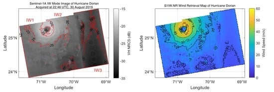
Figure 7a is the S1A IW mode VH-polarization image of Hurricane Dorian acquired at 22:46 UTC 30 August 2019. Figure 7b,c shows the wind speeds retrieved by the S1IW.NR model and the MS1A model. To ease visual comparison, the isopleth was drawn on those maps. Probability density distributions of VH NRCS and wind retrievals are shown in Figure 7d.
For wind speeds higher than 30 m/s, the areas in Figure 7b were larger than those in Figure 7c. In Figure 7d, the red solid curve was on the right side of the red dashed curve when wind speed was higher than 30 m/s. This indicates that the S1IW.NR model had higher retrievals than the MS1A model in a wind speed range from 30 to 60 m/s.
As shown in Figure 7d, although the wind speeds with maximum frequency for the two models were both between 10 and 20 m/s, their corresponding frequencies were quite different. The maximum frequency was 0.094 for S1IW.NR and 0.116 for MS1A, indicating their different performance under moderate wind condition (about 15 m/s).
In addition, S1IW.NR was able to detect the wind speeds lower than 10 m/s in IW1 and IW2. The areas of wind speeds lower than 10 m/s in Figure 7b were larger than those in Figure 7c, indicating that the S1IW.NR model had lower retrievals than the MS1A model under low wind condition (<10 m/s).
In summary, in this case, the wind speeds retrieved by S1IW.NR were distributed less uniformly. Meanwhile, the wind speeds retrieved by MS1A were more concentrated between 10 and 20 m/s. Compared with MS1A, S1IW.NR was more sensitive to wind speed lower than 10 m/s. This feature can also be seen in Figure 6. To note, the different performance of the two models shown in this case study corresponded to the curves’ difference illustrated in Figure 3. For both models, wind speeds changed smoothly at two adjacent sub-swath boundaries because the incident angle was considered during model development.
5. Discussion
Under TC conditions, extreme wind speed always appeared near the eyewall, where the rainfall was intense and random. The C-band radar’s signal was hardly affected by weak rainfall. However, due to the ambiguity of estimating and separating the contributions of precipitation from winds, eliminating intense rain impact on wind retrieval is still a problem [21].
Based on Dataset 2, 2305 collocated SFMR measurements of rainfall and wind speed were utilized to analyze the relationship between the S1IW.NR wind retrieval bias and rain rate between 0 and 48 mm/h. Their comparison is shown in Figure 8a. Probability density distributions of the two factors are shown in Figure 8b. Since there were few points with rain rate larger than 30 mm/h, the right Y-axis of Figure 8b was adjusted to 0–30 mm/h. The S1IW.NR wind retrieval bias was computed using Equation (9).
where is the wind speed retrieved by the S1IW.NR model and is the wind speed measured by SFMR.
Positive and negative biases both exist. For rain rate lower than 10 mm/h, 71.7% of the samples’ absolute values of bias were less than 5 m/s. The red trend line in Figure 8a illustrates that the retrieval bias increased with rain rate increasing from 10 to 35 mm/h. When rain rate was larger than 10 mm/h, retrieval biases of 71.1% samples were positive, indicating that the S1IW.NR model tends to overestimate wind speed under intense precipitation.
A bias of 11.5 m/s was reported at the rain rate of 35.7 mm/h. Its corresponding retrieved wind speed was 36 m/s. Thus, the impact of intense precipitation is not negligible for wind retrieval. Collocated rainfall information acquired by SFMR or other rain radar will contribute to flagging the possible errors.
6. Conclusions
SAR images and collocated wind references (i.e., SFMR and SMAP wind speed measurements) were collected for 12 TCs, in order to investigate the extreme wind speed retrieval utilizing the ESA Sentinel-1 IW mode product. Collocations were divided into two datasets. Dataset 1 was used to generate GMF, and Dataset 2 was used to validate the proposed GMF and carry out a case study.
The relationship between VH NRCS, ocean surface wind speed and incident angle was analyzed in a wind speed range from 10 to 74 m/s, based on 2783 matching points in Dataset 1. VH NRCS was not saturated even under extreme wind regime, increased with wind speed increasing, and varied with incident angle under low-to-moderate wind conditions. These relationships were different in each sub-swath.
A new GMF named S1IW.NR was then presented by curve fitting and regression correction. This empirical sub-swath-based GMF includes functions connecting VH NRCS to wind speed and incident angle. Using this GMF, extreme wind speeds can be retrieved from SAR imagery without external wind direction input. Compared with the Sentinel-1 observations, the VH NRCS simulated by the S1IW.NR model had an overall bias of 0.18 dB, a Cor of 0.80, and n RMSE of 1.86 dB, indicating the reliability of the fitting method we used.
For validation and comparison, we retrieved wind speeds from 3 to 53 m/s by the S1IW.NR model and the MS1A model and compared those retrievals with the SFMR wind speed measurements in Dataset 2. For all 2305 matching points, the bias, Cor, and RMSE of the S1IW.NR retrievals were −0.89 m/s, 0.89, and 4.13 m/s, respectively. It proves that the S1IW.NR model is able to retrieve extreme wind speeds with high accuracy. In addition, a case study of Hurricane Dorian was exploited to evaluate the performance of S1IW.NR and MS1A. Results showed that the proposed model was more accurate than MS1A.
Finally, the impact of rainfall on S1IW.NR wind retrieval was evaluated with the contribution of SFMR. Under rainfall, both positive and negative retrieval biases existed. Absolute value of bias increased with rain rate increasing from 10 to 35 mm/h. Retrieval biases of 71.1% samples were positive when the rain rate was over 10 mm/h, indicating that the proposed model tends to overestimate wind speed under intense rainfall. To explore the impact of rainfall on wind retrieval quantitatively, one possible way is to develop a combination of SAR and radiometer on board a new satellite.
Author Contributions
Initiation of the idea: Y.G.; Data processing and model proposing: Y.G.; Writing and editing: All authors contributed; Supervision: J.Z.; Funding acquisition: J.Z., J.S., and C.G. All authors have read and agreed to the published version of the manuscript.
Funding
This research was funded by the National Key Research and Development Program of China under grant 2016YFA0600102, the National Science Foundation of China under grants 61931025, U20A2099, and 41976017, the Fundamental Research Funds for the Central Universities under grant 20CX06109A, the Qingdao Postdoctoral Foundation Funded Project under grant qdyy20200098, and the China Postdoctoral Science Foundation Funded Project under grant 2020M682261.
Institutional Review Board Statement
Not applicable.
Informed Consent Statement
Not applicable.
Data Availability Statement
The data presented in this study are available on request from the author.
Acknowledgments
We thank the European Space Agency for making the Sentinel-1 products publicly available. We thank the National Oceanic and Atmospheric Administration for SFMR wind measurements and hurricane reports, the National Institute of Informatics and Meteo France for tracks of typhoon and Indian Ocean TC. SMAP sea surface wind data were produced by Remote Sensing Systems and sponsored by NASA Earth Science funding. Data are available at www.remss.com/missions/SMAP/winds/. We thank Remote Sensing Systems for SMAP wind data.
Conflicts of Interest
The authors declare no conflict of interest.
References
- Hersbach, H. Comparison of C-Band Scatterometer CMOD5.N Equivalent Neutral Winds with ECMWF. J. Atmos. Ocean. Technol. 2010, 27, 721–736. [Google Scholar] [CrossRef]
- Stoffelen, A.; Verspeek, J.A.; Vogelzang, J.; Verhoef, A. The CMOD7 Geophysical Model Function for ASCAT and ERS Wind Retrievals. IEEE J. Sel. Top. Appl. Earth Obs. Remote Sens. 2017, 10, 2123–2134. [Google Scholar] [CrossRef]
- Mouche, A.; Chapron, B. Global C-Band Envisat, RADARSAT-2 and Sentinel-1 SAR measurements in copolarization and cross-polarization. J. Geophys. Res. Ocean. 2016, 120, 7195–7207. [Google Scholar] [CrossRef] [Green Version]
- Lu, Y.; Zhang, B.; Perrie, W.; Mouche, A.; Wang, H. A C-band Geophysical Model Function for Determining Coastal Wind Speed Using Synthetic Aperture Radar. In Proceedings of the 2018 Progress in Electromagnetics Research Symposium (PIERS-Toyama), Tomaya, Japan, 1–4 August 2018. [Google Scholar] [CrossRef]
- Fernandez, D.E.; Carswell, J.R.; Frasier, S.; Chang, P.S.; Black, P.G.; Marks, F.D. Dual-polarized C- and Ku-band ocean backscatter response to hurricane-force winds. J. Geophys. Res. Atmos. 2006, 111. [Google Scholar] [CrossRef] [Green Version]
- Hwang, P.A.; Fois, F. Surface roughness and breaking wave properties retrieved from polarimetric microwave radar backscattering. J. Geophys. Res. Ocean. 2015, 120, 3640–3657. [Google Scholar] [CrossRef]
- Fois, F.; Hoogeboom, P.; Le Chevalier, F.; Stoffelen, A. Future Ocean Scatterometry: On the Use of Cross-Polar Scattering to Observe Very High Winds. IEEE Trans. Geosci. Remote Sens. 2015, 53, 5009–5020. [Google Scholar] [CrossRef]
- Horstmann, J.; Wackerman, C.; Falchetti, S.; Maresca, S. Tropical Cyclone Winds Retrieved from Synthetic Aperture Radar. Oceanography 2013, 26, 13962. [Google Scholar] [CrossRef] [Green Version]
- Shen, H.; Perrie, W.; He, Y. Evaluation of hurricane wind speed retrieval from cross-dual-pol SAR. Int. J. Remote Sens. 2016, 37, 599–614. [Google Scholar] [CrossRef]
- Ye, X.; Lin, M.; Zheng, Q.; Yuan, X.; Liang, C.; Zhang, B.; Zhang, J. A Typhoon Wind-Field Retrieval Method for the Dual-Polarization SAR Imagery. IEEE Geosci. Remote Sens. Lett. 2019, 16, 1511–1515. [Google Scholar] [CrossRef]
- Hwang, P.A.; Stoffelen, A.; Van Zadelhoff, G.J.; Perrie, W.; Zhang, B.; Li, H.; Shen, H. Cross-polarization geophysical model function for C-band radar backscattering from the ocean surface and wind speed retrieval. J. Geophys. Res. Ocean. 2015, 120, 893–909. [Google Scholar] [CrossRef]
- Shao, W.; Yuan, X.; Sheng, Y.; Sun, J.; Zhou, W.; Zhang, Q. Development of Wind Speed Retrieval from Cross-Polarization Chinese Gaofen-3 Synthetic Aperture Radar in Typhoons. Sensors 2018, 18, 412. [Google Scholar] [CrossRef] [Green Version]
- Shao, W.; Zhu, S.; Zhang, X.; Gou, S.; Zhao, L. Intelligent Wind Retrieval from Chinese Gaofen-3 SAR Imagery in Quad-Polarization. J. Atmos. Ocean. Technol. 2019, 36, 2121–2138. [Google Scholar] [CrossRef]
- Zhang, B.; Perrie, W. Recent progress on high wind-speed retrieval from multi-polarization SAR imagery: A review. Int. J. Remote Sens. 2014, 35, 4031–4045. [Google Scholar] [CrossRef]
- Huang, L.; Liu, B.; Li, X.; Zhang, Z.; Yu, W. Technical Evaluation of Sentinel-1 IW Mode Cross-Pol Radar Backscattering from the Ocean Surface in Moderate Wind Condition. Remote Sens. 2017, 9, 854. [Google Scholar] [CrossRef] [Green Version]
- Gao, Y.; Guan, C.; Sun, J.; Xie, L. A Wind Speed Retrieval Model for Sentinel-1A EW Mode Cross-Polarization Images. Remote Sens. 2019, 11, 153. [Google Scholar] [CrossRef] [Green Version]
- Gao, Y.; Guan, C.; Sun, J.; Xie, L. Tropical Cyclone Wind Speed Retrieval from Dual-polarization Sentinel-1 EW Mode Products. J. Atmos. Ocean. Technol. 2020, 7, 1713–1724. [Google Scholar] [CrossRef]
- Zhang, B.; Perrie, W.; Zhang, J.A.; Uhlhorn, E.W.; He, Y. High-Resolution Hurricane Vector Winds from C-Band Dual-Polarization SAR Observations. J. Atmos. Ocean. Technol. 2014, 31, 272–286. [Google Scholar] [CrossRef]
- Zhang, G.; Li, X.; Perrie, W.; Hwang, P.A.; Zhang, B.; Yang, X. A Hurricane Wind Speed Retrieval Model for C-Band RADARSAT-2 Cross-Polarization ScanSAR Images. IEEE Trans. Geosci. Remote Sens. 2017, 55, 4766–4774. [Google Scholar] [CrossRef]
- Mouche, A.; Chapron, B.; Zhang, B.; Husson, R. Combined Co- and Cross-Polarized SAR Measurements Under Extreme Wind Conditions. IEEE Trans. Geosci. Remote Sens. 2017, 55, 6746–6755. [Google Scholar] [CrossRef]
- Mouche, A.; Chapron, B.; Knaff, J.; Zhao, Y.; Zhang, B.; Combot, C. Co- and Cross- polarized SAR measurements for high resolution description of major hurricane wind structures: Application to Irma category-5 Hurricane. J. Geophys. Res. Ocean. 2019, 124, 3905–3922. [Google Scholar] [CrossRef]
- Zhang, K.; Huang, J.; Mansaray, L.R.; Guo, Q.; Wang, X. Developing a Subswath-Based Wind Speed Retrieval Model for Sentinel-1 VH-Polarized SAR Data Over the Ocean Surface. IEEE Trans. Geosci. Remote Sens. 2018, 57, 1561–1572. [Google Scholar] [CrossRef]
- Zhang, G.; Li, X.; Perrie, W. Synthetic Aperture Radar Observations of Extreme Hurricane Wind and Rain. In Hurricane Monitoring with Spaceborne Synthetic Aperture Radar; Springer: Singapore, 2017. [Google Scholar]
- Long, D.G.; Nie, C. Hurricane Precipitation Observed by SAR. In Hurricane Monitoring with Spaceborne Synthetic Aperture Radar; Springer: Singapore, 2017. [Google Scholar]
- Moore, R.; Yu, Y.; Fung, A.; Kaneko, D.; Dome, G.; Werp, R. Preliminary study of rain effects on radar scattering from water surfaces. IEEE J. Ocean. Eng. 2003, 4, 31–32. [Google Scholar] [CrossRef]
- Zhang, G.; Li, X.; Perrie, W.; Zhang, B.; Lei, W. Rain effects on the hurricane observations over the ocean by C-band Synthetic Aperture Radar. J. Geophys. Res. Ocean. 2016, 121, 14–26. [Google Scholar] [CrossRef] [Green Version]
- Uhlhorn, E.W.; Black, P.G.; Franklin, J.L.; Goodberlet, M.; Carswell, J.; Goldstein, A.S. Hurricane Surface Wind Measurements from an Operational Stepped Frequency Microwave Radiometer. Mon. Wea. Rev. 2007, 135, 3070–3085. [Google Scholar] [CrossRef] [Green Version]
- Klotz, B.W.; Uhlhorn, E.W. Improved Stepped Frequency Microwave Radiometer Tropical Cyclone Surface Winds in Heavy Precipitation. J. Atmos. Ocean. Technol. 2014, 31, 2392–2408. [Google Scholar] [CrossRef]
- Meissner, T.; Wentz, F.J.; Ricciardulli, L. The emission and scattering of L-band microwave radiation from rough ocean surfaces and wind speed measurements from the Aquarius sensor. J. Geophys. Res. Ocean. 2015, 119, 6499–6522. [Google Scholar] [CrossRef]
- Meissner, T.; Ricciardulli, L.; Wentz, F.J. Capability of the SMAP Mission to Measure Ocean Surface Winds in Storms. Bull. Amer. Meteor. Soc. 2017, 98, 1660–1677. [Google Scholar] [CrossRef]
- Zhang, B.; Perrie, W. Cross-Polarized Synthetic Aperture Radar: A New Potential Measurement Technique for Hurricanes. Bull. Amer. Meteor. Soc. 2012, 93, 531–541. [Google Scholar] [CrossRef] [Green Version]
Figure 1.
The numbers of matching points in different wind regimes and different sub-swaths. D1 and D2 are short for Dataset 1 and Dataset 2. IW1, IW2, and IW3 stand for sub-swath 1, sub-swath 2, and sub-swath 3, respectively.
Figure 1.
The numbers of matching points in different wind regimes and different sub-swaths. D1 and D2 are short for Dataset 1 and Dataset 2. IW1, IW2, and IW3 stand for sub-swath 1, sub-swath 2, and sub-swath 3, respectively.

Figure 2.
The distributions of VH NRCS, incident angle, and wind speed in different sub-swaths in Dataset 1. The total number of matching points was 2783.
Figure 2.
The distributions of VH NRCS, incident angle, and wind speed in different sub-swaths in Dataset 1. The total number of matching points was 2783.

Figure 3.
Comparison between VH NRCS and wind speed in (a) IW1; (b) IW2; (c) IW3. Matching points from SMAP and SFMR are colored by blue and green.
Figure 3.
Comparison between VH NRCS and wind speed in (a) IW1; (b) IW2; (c) IW3. Matching points from SMAP and SFMR are colored by blue and green.


Figure 4.
The difference between SAR-observed and Equation (5)-simulated VH NRCS for wind speeds less than 30 m/s under different incident angles.
Figure 4.
The difference between SAR-observed and Equation (5)-simulated VH NRCS for wind speeds less than 30 m/s under different incident angles.

Figure 5.
Comparison between the VH NRCS values simulated by S1IW.NR and observed by Sentinel-1 SAR in Dataset 1. Red, green, and blue circles stand for samples in IW1, IW2, and IW3, respectively.
Figure 5.
Comparison between the VH NRCS values simulated by S1IW.NR and observed by Sentinel-1 SAR in Dataset 1. Red, green, and blue circles stand for samples in IW1, IW2, and IW3, respectively.

Figure 6.
Comparison between the wind speed retrievals and SFMR measurements based on Dataset 2. Wind speeds were retrieved by the (a) S1IW.NR model and (b) MS1A model. Red, green, and blue points stand for IW1, IW2, and IW3, respectively.
Figure 6.
Comparison between the wind speed retrievals and SFMR measurements based on Dataset 2. Wind speeds were retrieved by the (a) S1IW.NR model and (b) MS1A model. Red, green, and blue points stand for IW1, IW2, and IW3, respectively.

Figure 7.
(a) S1A IW mode VH-polarization image of Hurricane Dorian acquired at 22:46 UTC 30 August 2019. Wind speed retrievals of Hurricane Dorian using (b) the S1IW.NR model and (c) the MS1A model. (d) The probability density distribution of VH NRCS in (a) and wind speeds in (b,c). In (d), the red solid curve and red dashed curve stand for the wind speeds retrieved by S1IW.NR and MS1A, corresponding to the left Y-axis. Black curve stands for the VH NRCS, corresponding to the right Y-axis.

Figure 8.
(a) Comparison and (b) probability density distribution of the S1IW.NR wind retrieval bias and the SFMR-measured rain rate based on Dataset 2. The red curve in (a) stands for the trend of bias changing with rain rate. In (b), the red curve is the frequency of the S1IW.NR wind speed bias, corresponding to the left Y-axis. The black curve is the frequency of the SFMR-measured rain rate, corresponding to the right Y-axis.


Table 1.
Information of TCs, SAR images, and wind references.
| TC Name | Category | SAR Instrument | SAR Acquisition Time (UTC) | Wind Reference | Dataset |
|---|---|---|---|---|---|
| Irma | 5 | S1A | 2017/09/07 10:29 | SFMR | 1 |
| Maria | 3 | S1A | 2017/09/21 22:45 | SMAP | 1 |
| Trami | 2 | S1B | 2018/09/29 09:27 | SMAP | 1 |
| Idai | 5 | S1A | 2019/03/14 16:06 | SMAP | 1 |
| Dorian | 4 | S1A | 2019/08/30 22:46 | SFMR | 2 (Case Study) |
| 3 | S1A | 2019/09/03 11:17 | SMAP SFMR | 1 2 | |
| 1 | S1A | 2019/09/07 21:46 | SMAP | 1 | |
| Humberto | TS | S1A | 2019/09/14 23:11 | SMAP | 1 |
| Isaias | TS | S1B | 2020/08/02 23:20 | SFMR | 2 |
| Chan-Hom | TS | S1B | 2020/10/06 20:45 | SMAP | 1 |
| Delta | 1 | S1B | 2020/10/08 00:07 | SFMR | 2 |
| 3 | S1A | 2020/10/09 12:07 | SFMR | 1 |
Table 2.
Comparison of data sources of the proposed S1IW.NR model, the MS1A model, and the S-C2PO model.
Table 2.
Comparison of data sources of the proposed S1IW.NR model, the MS1A model, and the S-C2PO model.
| GMF | SAR Mode | Resampling SAR Data Resolution (km) | Wind Reference |
|---|---|---|---|
| S1IW.NR | IW | 25, 1 | SMAP, SFMR |
| MS1A | EW | 40 | SMAP |
| S-C2PO | IW | 5 | CMOD5.N Retrieval |
Table 3.
Validation results of the proposed S1IW.NR model with the SFMR wind speed references and comparison with the MS1A model based on Dataset 2.
Table 3.
Validation results of the proposed S1IW.NR model with the SFMR wind speed references and comparison with the MS1A model based on Dataset 2.
| Sub-swath | Points Number | Bias (m/s) | Cor | RMSE (m/s) | |||
|---|---|---|---|---|---|---|---|
| S1IW.NR | MS1A | S1IW.NR | MS1A | S1IW.NR | MS1A | ||
| IW1 | 528 | −0.25 | −0.91 | 0.89 | 0.90 | 4.40 | 3.88 |
| IW2 | 968 | 0.50 | −1.68 | 0.93 | 0.93 | 3.89 | 3.89 |
| IW3 | 809 | −2.89 | −3.82 | 0.63 | 0.61 | 4.18 | 4.63 |
| IW1—3 | 2305 | −0.89 | −2.31 | 0.89 | 0.89 | 4.13 | 4.25 |
Publisher’s Note: MDPI stays neutral with regard to jurisdictional claims in published maps and institutional affiliations. |
© 2021 by the authors. Licensee MDPI, Basel, Switzerland. This article is an open access article distributed under the terms and conditions of the Creative Commons Attribution (CC BY) license (https://creativecommons.org/licenses/by/4.0/).
Share and Cite
MDPI and ACS Style
Gao, Y.; Sun, J.; Zhang, J.; Guan, C. Extreme Wind Speeds Retrieval Using Sentinel-1 IW Mode SAR Data. Remote Sens. 2021, 13, 1867. https://doi.org/10.3390/rs13101867
AMA Style
Gao Y, Sun J, Zhang J, Guan C. Extreme Wind Speeds Retrieval Using Sentinel-1 IW Mode SAR Data. Remote Sensing. 2021; 13(10):1867. https://doi.org/10.3390/rs13101867
Chicago/Turabian StyleGao, Yuan, Jian Sun, Jie Zhang, and Changlong Guan. 2021. "Extreme Wind Speeds Retrieval Using Sentinel-1 IW Mode SAR Data" Remote Sensing 13, no. 10: 1867. https://doi.org/10.3390/rs13101867
Note that from the first issue of 2016, this journal uses article numbers instead of page numbers. See further details here.