Article

Improved Accuracy of Riparian Zone Mapping Using Near Ground Unmanned Aerial Vehicle and Photogrammetry Method

1
Faculty of Forestry and Environmental Management, University of New Brunswick, Fredericton, NB E3B 5A3, Canada
2
Department of Animal Science, Faculty of Agricultural and Food Sciences, University of Manitoba, Winnipeg, MB R3T 2N2, Canada
3
Agriculture and Agri-Food Canada, Fredericton Research and Development Centre, 850 Lincoln Road, Fredericton, NB E3B 4Z7, Canada
*
Author to whom correspondence should be addressed.
Remote Sens. 2021, 13(10), 1997; https://doi.org/10.3390/rs13101997
Submission received: 1 April 2021 / Revised: 14 May 2021 / Accepted: 18 May 2021 / Published: 20 May 2021

Abstract

:
In agriculture-dominant watersheds, riparian ecosystems provide a wide array of benefits such as reducing soil erosion, filtering chemical compounds, and retaining sediments. Traditionally, the boundaries of riparian zones could be estimated from Digital Elevation Models (DEMs) or field surveys. In this study, we used an Unmanned Aerial Vehicle (UAV) and photogrammetry method to map the boundaries of riparian zones. We first obtained the 3D digital surface model with a UAV. We applied the Vertical Distance to Channel Network (VDTCN) as a classifier to delineate the boundaries of the riparian area in an agricultural watershed. The same method was also used with a low-resolution DEM obtained with traditional photogrammetry and two more LiDAR-derived DEMs, and the results of different methods were compared. Results indicated that higher resolution UAV-derived DEM achieved a high agreement with the field-measured riparian zone. The accuracy achieved (Kappa Coefficient, KC = 63%) with the UAV-derived DEM was comparable with high-resolution LiDAR-derived DEMs and significantly higher than the prediction accuracy based on traditional low-resolution DEMs obtained with high altitude aerial photos (KC = 25%). We also found that the presence of a dense herbaceous layer on the ground could cause errors in riparian zone delineation with VDTCN for both low altitude UAV and LiDAR data. Nevertheless, the study indicated that using the VDTCN as a classifier combined with a UAV-derived DEM is a suitable approach for mapping riparian zones and can be used for precision agriculture and environmental protection over agricultural landscapes.

1. Introduction

Riparian zones are vegetated areas adjacent to natural water bodies with distinctive plant communities different from their upland surroundings, strongly shaped and affected by geomorphic processes occurring in the area [1,2,3]. The critical location of riparian zones within watersheds allows them to intercept pollutants received from uplands and prevent these pollutants from transferring downstream to estuarine systems [4,5,6,7]. The volume of water, as well as its pathways moving through the riparian zones, are fundamental for understanding nutrient removal and retention [8].
From a resource management perspective, valley bottoms are often focal points of conflict between human land uses and the protection of vulnerable riparian ecotones. Harvest operations and agriculture practices can lead to deleterious effects on the stream channel. The removal of streamside vegetation not only compromises the stabilization effects of roots upon the bank soil but also reduces the hydraulic roughness of the bank, which could lead to a rise in flow velocities [9] and thus accelerate channel erosion and increase sediment input into streams [10,11]. In addition, failing riparian ecosystems cannot buffer streams against sediment and pollutants loading from uplands.
The effectiveness of riparian conservation depends largely on the accurate delineation of the riparian zone. Traditionally, riparian zone delineations have been concentrated on field measurements over a few hundred meters [10,12]. This task could be time-consuming and labor-intensive to evaluate a large area such as an entire catchment or a long river corridor, particularly in remote locations. One way to reduce the time and costs is to sample representative sections. However, the selection of representative sites can suffer from subjectivity and be limited by accessibility and safety, which could introduce large uncertainties for the full characterization of a riparian zone [13].
Remote sensing techniques have been used to map riparian zones due to their advantages in spatial extensiveness, non-invasiveness, and repeatability [14,15]. Riparian zones can be mapped by predicting the interface between permanently wet or wetter areas due to position in the landscape using terrain attributes, such as slope gradient and elevation [16,17], and/or the presence of a permanent or fluctuating water table near the soil surface, terrain wetness index and local drainage patterns, or proximity to a watercourse. Concurrently, these factors are prone to develop a specific soil type, describing the spatial variation and distribution of saturated soils in a particular landscape.
Researchers and conservationists have attempted to map the complex soil drainage classes and riparian ecosystems using online geospatial datasets [18,19,20]. This often means the usage of coarser-resolution spatial data collected from traditional photogrammetry, offering inaccurate results when attempting to represent lower-order streams and small watersheds [21,22]. Conventional low-resolution DEMs are also unable to capture topographic variations in detail. For example, Murphy et al. [20] concluded that the final map imperfections and limitations were probably the result of the poorer resolution and lower initial elevation point density of these topographic models. Therefore, for ecosystem protection, restoration, and management at smaller scales, more accurate and detailed DEMs have become necessary [23,24].
Light Detection and Ranging (LiDAR) technology can collect high density elevation points, which has been used to generate DEMs with more topographic detail and lead to improved hydrological modeling accuracy. Buchanan, et al. [25] concluded that using a high-resolution DEM (3 m) provided better results than using a 10 m resolution DEM when estimating soil moisture conditions using a topographic wetness index. The spatial resolution and data format have a significant impact on predicting the parameters mentioned to represent the boundaries of ecotones with different soil moisture regimes.
Bock and Köthe [26] postulated that soil characteristics influenced by groundwater hydrological processes could be mapped according to the Vertical Distance to Channel Network (VDTCN), a topographic index that reflects the average groundwater table depth based on topographic positions and the distance to existing flow channels. A similar method was used to investigate the spatial distribution of soil properties in relation to micro-topography using a 1m resolution DEM [27], or 25 m DEM [28].
Recent technological advances, as well as the increasing availability of Unmanned Aerial Vehicles (UAVs) with multimodal sensors, coupled with improved photogrammetry and computer algorithms have led to dramatic improvements in the collection and processing of terrain data using photogrammetry. This approach can produce high resolution Digital Surface Models (DSMs) with high quality and makes UAVs a cost-effective alternative to Airborne Laser Scanning (ALS) [29,30,31]. Jeziorska [32] assessed the suitability of DEMs obtained from UAV photogrammetry for overland flow simulations in the context of precision agriculture applications. They concluded that UAV-based data were most suitable for overland flow predictions compared with other methods including LiDAR data. Rahman, et al. [33] combined orthophotography and photogrammetric point clouds acquired from UAVs to map peatland groundwater table in the Peace River area (Alberta, Canada). By identifying pockets of surface water, they obtained a direct measurement of groundwater level (GWL) in locations where it was visible and generated continuous-surface estimates over large areas through interpolation [33].
The general objective of this study was to test the feasibility of using a near ground UAV and photogrammetry method for riparian zone mapping. Specific objectives included: (1) Collecting high resolution DEM data using a UAV and photogrammetry method; (2) Using high resolution DEMs to classify riparian zones in agricultural landscapes with Vertical Distance to Channel Network; (3) Estimating optimal parameters for riparian zone delineation with DEM; (4) Assessing the accuracy of riparian zone delineation with different DEM resolutions and data sources.

2. Materials and Methods
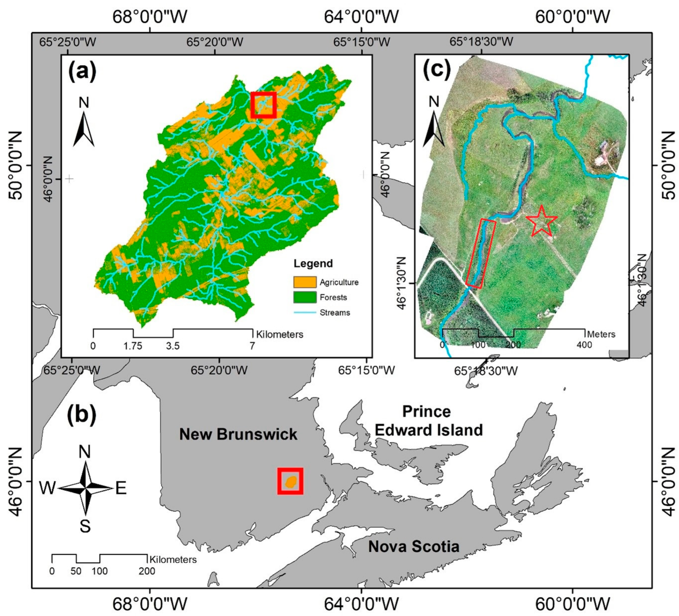
2.1. Study Area

The study area is located on the Ridge Brook, within the Canaan River Watershed, near Havelock in the province of New Brunswick, Canada (46°01′29.0″N, 65°18′32.5″W; Figure 1). The Ridge Brook sub-watershed covers an area of 7020 ha. Land use within the watershed is primarily agriculture, with small scale limestone extraction operation near the small town of Havelock.
The farm where the study was conducted grows a mix crops, including grasses, barley, and legumes. The soil type has been classified as Luvisolic, which has a forest mull Ah, and a Bt or Btg horizons. The Ah horizon is the top mineral soil horizon enriched with organic matter. While the Bt horizon is an illuvial horizon enriched with silicate clay, normally formed below an eluvial horizon, the “Btg” horizon indicates poor drainage and periodic reduction due to significant amount of clay accumulation. Therefore, gleying (anoxic) conditions are likely to occur within 50 cm of the mineral surface, and these features can be found particularly in depressions with poorly drained sites coupled with Regosolic soils. Soils in certain areas lack a distinguished “B” horizon of at least 5 cm, probably due to recent alluvium, or colluvium on slopes, in which case the nature of the material can be purely quartz sand. These types of soils are often classified as rapidly to imperfectly drained (Canadian soil classification system). The pH detected in the field is close to 5.5. The upstream riparian area adjacent to the farm is surrounded by two sections of planted conifer species, red pine (Pinus resinosa) and Jack pine (Pinus banksiana). These planted species may increase the acidity of the soil in the natural riparian forest, located in the southernmost part of the study area.
Prior to 2007, cattle had access to the stream as a watering source and used the riparian zone for grazing. These cattle activities caused some impacts on the structural integrity of the stream banks and the growth of riparian vegetation, which led to a widening of the channel and increased sedimentation. In 2007, a bioengineered buffer zone—that currently covers approximately one-third of the stream path through the farm—was implemented to increase riparian health, to add stability to the stream, and to recover the riparian zone to a more natural condition. With the help of a bioengineered buffer zone protection project, the vegetation coverage increased as well as the bank stability, and reduced eutrophication due to accelerating the water velocity. However, due to the lack of an off-stream watering system for cattle and absence of a dedicated livestock crossing, vegetation is still removed from grazing activities in the areas outside of the bioengineered buffer. Cattle activities have also caused soil compaction along the fenced area on the eastern side of the stream.

2.2. Functional Riparian Zone Delineation

2.2.1. Online Available Data Interpolation

The traditional coarse resolution provincial DEM was obtained from the Service New Brunswick (SNB) geographic information source (http://www.snb.ca/geonb1/e/DC/DEM.asp, accessed on 1 April 2021). The accuracy of a single elevation point was approximately 2.5 m and the spacing between the elevation points was of nearly 70 m on average, with increased density in more complex terrain area. We generated a DEM at a 2 m cell size using the Inverted Distance Weighted (IDW). This DEM was hydrologically corrected in ArcMap 10.5 with field-mapped open drainage channel network ("burn" DEM) within the Service New Brunswick Geospatial Database.
The LiDAR DEMs were obtained from the Service New Brunswick Geospatial Database. The point cloud density of the LiDAR dataset collected in 2013 was 1.2 points m−2. The DEM based on the 2013 LiDAR data had a horizontal accuracy of 0.3 m and the vertical accuracy of 0.133 m at 95% confidence level. The point cloud density of LiDAR dataset collected in 2018 was 6 points m−2. The horizontal accuracy was 0.20 m, and vertical accuracy was RMSE Z = 10.5 cm, equating to +/− 20.6 cm at a 95% confidence level. The DEM raster was generated with Natural Neighbors interpolation with a 30 cm resolution.

2.2.2. UAV and Sensor Description

The Unmanned Aerial Vehicle (UAV) used in this study was a DJI Phantom 4 Pro (Da-Jiang Innovations, SZ DJI Technology Co., LTD; Figure 2). This UAV was chosen due to its recognized camera stability which is considered to be a key factor for precision agriculture and forestry purposes [34,35,36]. The Phantom 4 Pro is a vertical takeoff and landing aircraft with total payload of 1388 g, battery and propellers included. This UAV uses four 2312S Brushless motors powered by a 15.2 V battery with a cruising speed of 72.0 km h−1 (s-mode) and a maximum climb speed of 6 m s−1. The maximum service ceiling is 6000 m asl and the maximum transmission range with no obstruction and free of interference is up to 7 km. The maximum payload is 1.02 lbs. The maximum wind speed resistance is up to 10.0 m s−1. The reported maximum flight time with a single battery is 30 min, with a practical flying time of around 25 min based on our tests depending on wind speed and temperature (<10 km h−1; > 4 °C). We planned the flight durations within 20 min, at a flight speed of 7 m s−1.
The onboard camera is 1 inch complementary metal oxide semiconductor (CMOS) with 20 M effective pixels (5472 × 3648). The lens has a field of view (FOV) of 84° and the focal length is 8.8 mm/24 mm (35 mm format equivalent) f/2.8–f/11 auto focus at 1 m–∞. During the flight, the sensor registers either vertical images captured at Nadir angle (for 2D maps), or the camera can be tilted (off-Nadir angles) up to 90 degrees for 3D Digital Surface Model (DSM) reconstructions. The image trigger can be activated automatically in autopilot flight mode, with simultaneous timestamps and automatic recording of GPS locations due to its multiple satellite position navigation system (GPS and GLONASS). The reported vertical hover accuracy range is 0.5 m with GPS positioning and the horizontal hover accuracy is 1.5 m with GPS positioning. Images and metadata are automatically stored with a 64 GB Lexar high performance 633x MicroSDXC UHS-I Secure Digial Card (SD-Card).
Rogers et al. [37] tested different UAVs (DJI Inspire 1, DJI Mavic Pro, and DJI Matrice 210) including DJI Phantom 4 Pro and compared the accuracy of the UAV-derived DSMs for each UAV using a DSM created from Light Detection and Ranging (LiDAR) mounted on a DJI Matrice 600 Pro. They found that the DJI Phantom 4 pro provided higher accuracy in four of the six land covers tested (vines, bare soil, forest, and mowed grass). Among the drones tested, the DJI Phantom 4 Pro performed the best due to the higher resolution sensor (20 MP), which provides finer Ground Sample Distances (GSDs) and greater density in output point clouds. They also ranked the UAVs used in different categories, including maximum flight time, number of batteries, dimensions, resolution, and weight. The Phantom 4 Pro was considered to be the best balance between size and sensor resolution, which makes this a versatile drone widely used by professional users [37].

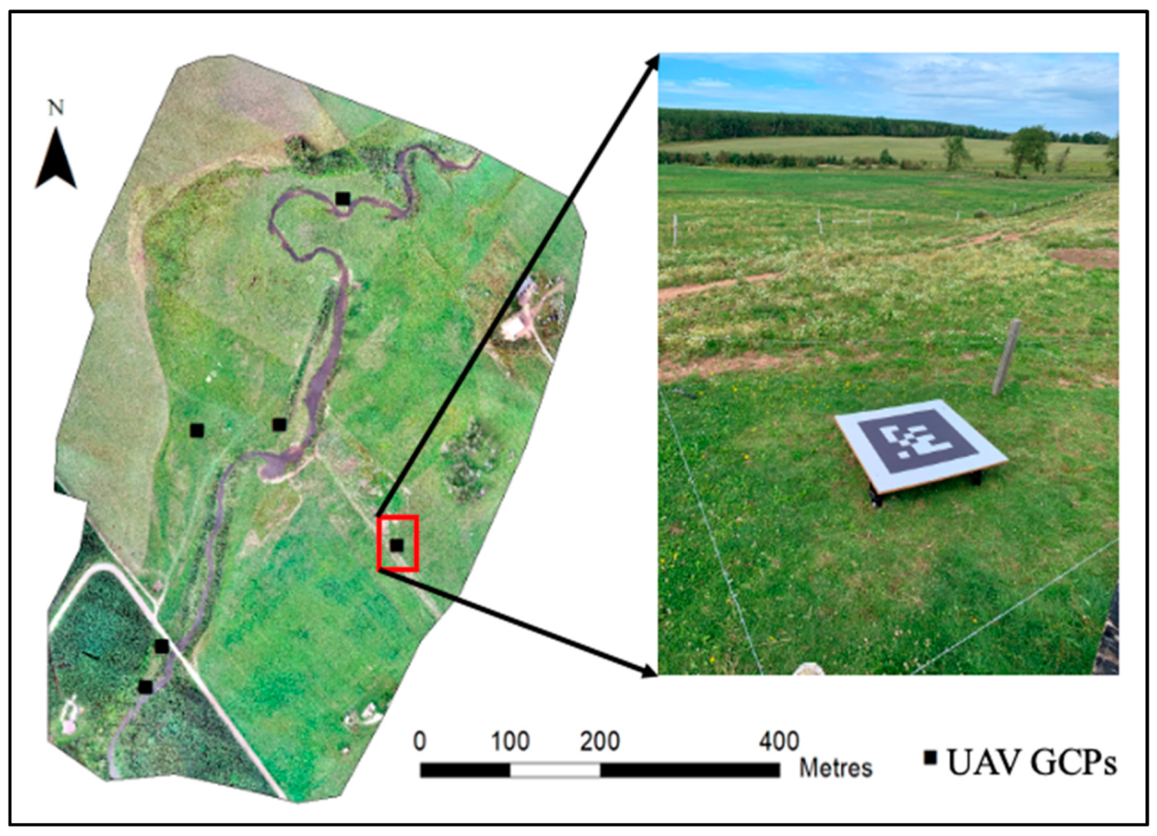
2.2.3. UAV Data Collection

Flights and image acquisition were scheduled on days when the temperature was above 5 °C and the wind speed was low (<10 km h−1). We tried capturing images under overcast or partially overcast days to minimize shading effects. We acquired near-ground UAV aerial data in 2018 and 2019 in three different seasons, including early Spring, Summer, and Fall (8 May, 20 August, and 17 November of 2018, and 13 May, 28 August, and 25 October of 2019). The main consideration of season selection was to map different vegetation growth stages and streamflow conditions throughout the year. The early spring provided field conditions with herbaceous vegetation that was still snow-flattened but without snow cover on the ground. This can reduce the elevation error caused by the height of streamside vegetation. Deciduous tree species were also still in leaf-off conditions. These data can be used to visually identify the starting points of ephemeral, intermittent, or permanent flows and help in determining the threshold parameter of streams for flow accumulation data. The stream initiation parameter is an important parameter for the mapping of lower-order stream network-based DEM, and it is difficult to determine due to upland variations in vegetation cover and type, topography, sediment, and soil hydraulic properties across regions due to variations in weather and climate [38,39].
Six ground control markers (square targets of 1.44 m2) were equally positioned across the site and at the boundaries of the UAV study area, including next to the watercourse at different elevations (Figure 3). A ground control point (GCP) of each target’s corners was recorded with a Trimble Geoexplorer 6000 Series handheld GPS (10 cm of horizontal accuracy according to the GPS manual) to mark the positions of the panels with geometrical precision for georeferencing accuracy. Each position was registered using the real-time kinematics (RTK) mode to register the location of each target (checkpoint). To do so, the GPS was placed in a static position for 30 seconds. The precision observed in the GPS device during the geolocation acquisition was 10 cm for each record, with a minimum of 16 satellites available.
During each flight, we acquired 1027 images following pre-planned and evenly spaced parallel flight paths in two directions to form a squared grid using Pix4D app (Pix4D Inc). The side and frontal overlap rate was 80%. The average flight speed was 7 m s−1 at near ground elevation (80 m), with the camera set at Nadir angle for 2D mapping. The captured images were processed with the Structure from Motion (SfM) algorithm to generate geo-rectified orthomosaic images using Pix4D 4.4 (Pix4D Inc). The latitude, longitude, and altitude (WGS84 projection) in metadata were used to position the aerial photos first. Common points from different images in the overlap areas were used as keypoints to build a 3D projected point through aerotriangulation [40]. In order to improve the software image stitching, 10 manual tie points (mtps) were added in the planted forest area upstream.

2.2.4. Point Cloud Cleaning

We observed that 3D information on water surfaces had a large error, potentially caused by floating objects moving on the water’s surface as well as light/illumination changes between images captured at different times (i.e., reflection, absorption, and refraction). The camera could also penetrate the water surface to identify the stream bed in some cases but not in others, and this caused large errors or noise in surface elevation. Points classified as water were removed in order to reduce the uncertainties for the estimation of the stream channel, the triangulation, and the effects on the quality of the DEM [41]. In addition, misclassification for ground or vegetation was manually corrected to avoid errors in the surface model [42]. The resulting point cloud had an average density of 833 points m−2, and it was further interpolated at 0.3 m resolution, using the LAStools commercial software suite (Martin Isenburg, LAStools -efficient tools for LiDAR processing).

2.2.5. Stream Network and Flow Initiation Thresholds

The spatial hydrology tools of ArcGIS (10.5) were used to generate stream networks. For the traditional coarse resolution DEM, the existing stream network was used to correct the flow patterns in the flow accumulation raster [43]. This is necessary because a coarse-resolution DEM could not capture and represent the topographic features, such as small streams, due to interpolation errors [44]. Because of their greater initial point density, LiDAR and UAV DEMs do not require stream correction. Local depressions or sinks were removed with a fill function to create a depressionless DEM. The flow direction rasters were produced with a D8 algorithm [45]. The flow accumulation raster was derived from the flow direction raster. The flow accumulation raster was used to derive low order stream network according to the predefined flow initiation threshold. The flow initiation threshold was used as a parameter to optimize riparian zone mapping accuracy.

2.2.6. Functional Riparian Prediction

The Vertical Distance to Channel Network (VDTCN) was used as a classifier for riparian zones. The Vertical Distance to Channel Network parameter measures the relative elevation difference between a point of interest to the elevation of the channel network. The parameter algorithm has been successful in inferring groundwater levels, aiding soil mapping processes, and predicting soil textures [26]. More specifically, the tool uses an algorithm that consists of two major steps: (1) It interpolates the elevation of streams and creates a base level elevation of the stream network; (2) the neighboring stream cells for points of interest are determined iteratively using the distance from the center of the cell as a weighting factor. The final VDTCN is calculated by subtracting this base level from the re-calculated DEM neighboring elevations [26].

2.2.7. Field Validation

The indicator of vegetation species adapted to poorly drained and wetted soils could also be used to identify riparian areas because these vegetation species rely on access to groundwater [46,47]. In this study, sedges (Carex sp.), rushes (Juncus sp.), grasses (Panicum sp. or Agropyron sp.), blue flag iris (Iris versicolor), and cattails (Typha sp.) were used as indicators species to map the riparian zone since they are known to grow in partially submerged and water-logged riparian soils. Sites with over 50% visual cover [48] of target species were included within the riparian field delineation.
In areas absence of hydrophytic vegetation, soil with signs of groundwater table fluctuations was used to identify riparian areas [49]. Fifty-four soil pits were dug in transects of 5 m increments from the highly dense riparian vegetation boundaries. The soil indicators include signs of anaerobic conditions, such as the existence of microbially reduced ferrous (Fe2+) from ferric iron (Fe3+), the presence of organic carbon, and grey matrix soil color caused by elluviation. In addition, redoximorphic features, such as mottling and precipitation of manganese, were also used to identify the soils exposed to periodic or prolonged periods of saturation, typical in riparian zones [50]. A field survey of soil and vegetation indicators was used to register the boundary of the functional riparian zone using a handheld GPS (Trimble Geoexplorer 6000 Series). Figure 4 details the flowchart of the methodology.

2.2.8. Statistical Analysis

The quantitative consistency and correctness achieved by VDTCN with each DEM used as a source, compared with field survey, was calculated using the Kappa Index [51].

3. Results

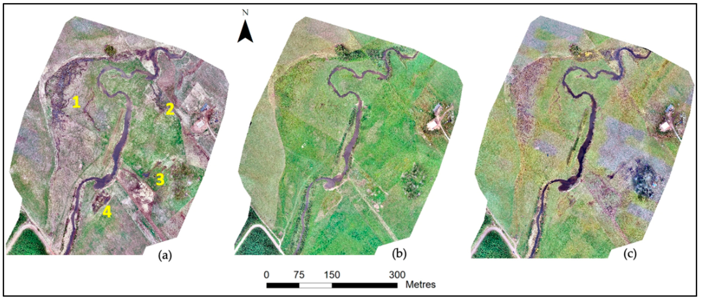
3.1. Interpolated DEMs and Geolocation Precision

The interpolated DEMs from point clouds of different sources are shown in Figure 5. As shown, the coarse DEM was visually different compared to the three high-resolution DEMs and could not represent the minor topographic features, including streams. No relevant elevation differences were observed between the LiDAR 1.2 and LiDAR 6.0-derived DEMs. The height values shown for the UAV-derived DEM were practically equal to the LiDAR values. On average, we obtained 53,566 keypoints per image and a minimum of five images overlapping every pixel. Since the Phantom 4 Pro is capable of automatically recording GPS locations, we used this product as the relative geolocation. As reported by Fabian, et al. [52], adverse factors, such as lens distortion, GPS position error, aircraft attitude uncertainty, and errors in the time domain can lead to the decreased accuracy in the relative UAV map geolocation. Therefore, we corrected the overall geolocation using the target coordinates, as checkpoints, acquired with handheld GPS as relative accuracy. The elevation Root Mean Squared Error (RMSE) for these GCPs was 0.075 meters, and the horizontal RMSE for longitude and latitude were 0.078 and 0.066 meters, respectively. These results indicate high precision between the measured coordinates (GCPs registered in the field) compared with the software-calculated position.

3.2. The Optimal Parameter for Riparian Zone Delineation

Since the traditional coarse resolution, DEM was the most available data; we optimized the flow initiation and VDTCN threshold parameters with this topographic model first. The flow network and VDTCN based on coarse resolution DEM with different flow initiation thresholds are shown in Figure 6. The UAV images obtained in Spring, Summer, and Fall are shown in Figure 7. As shown, the length of flow lines increases with decreased flow initiation thresholds (Figure 6a–c). To do so, we maximized the coinciding areas and minimized errors of commission (false positive) and omission (false negative), testing different minimum flow initiation and VDTCN thresholds (Figure 6). Higher VDTCN thresholds included more areas classified as wet (Figure 6d–f). We found that the optimal flow initiation threshold was 1.5 ha, and the optimal VDTCN threshold was 14.2 m. Afterward, we applied these optimized parameters found in the coarse resolution DEM to all other DEMs to predict the extents of riparian zones using LiDAR- and UAV-derived DEMs.
The riparian zone prediction accuracies measured as Kappa Coefficients (KC) are shown in Table 1. The Kappa Coefficent was 0.25 for the coarse-resolution DEM. When the optimal parameters derived from the coarse resolution DEM were directly applied to high-resolution DEMs, the KC were 0.04, 0.03, and 0.03 for LiDAR 1.2, LiDAR 6.0, and UAV DEMs, respectively. The coarse resolution DEM achieved a higher prediction accuracy than higher resolution DEMs. These results indicated that optimal parameters obtained with coarse resolution DEM could not be directly used to classify riparian zones with high-resolution DEMs.
The flow network and VDTCN based on high-resolution DEMs with different flow initiation thresholds are shown in Figure 8. The accuracies of riparian zone prediction with different DEMs and different flow initiations are shown in Table 1. For the LiDAR1.2 DEM, we found the optimal flow initiation threshold was 0.75 ha, and the optimal VDTCN threshold was 0.4 m, and we achieved a KC of 0.63. If the optimal parameters found for LiDAR1.2 DEM were used for LiDAR6 and UAV DEMs, the KC were 0.63 and 0.56, respectively (Table 1). These results confirmed that the optimal parameters for the prediction of riparian zones with different DEMs are not the same and could not be used interchangeably. With the UAV DEM, the optimal flow initiation threshold was 0.50 ha, and the VDTCN threshold was 0.48 m.

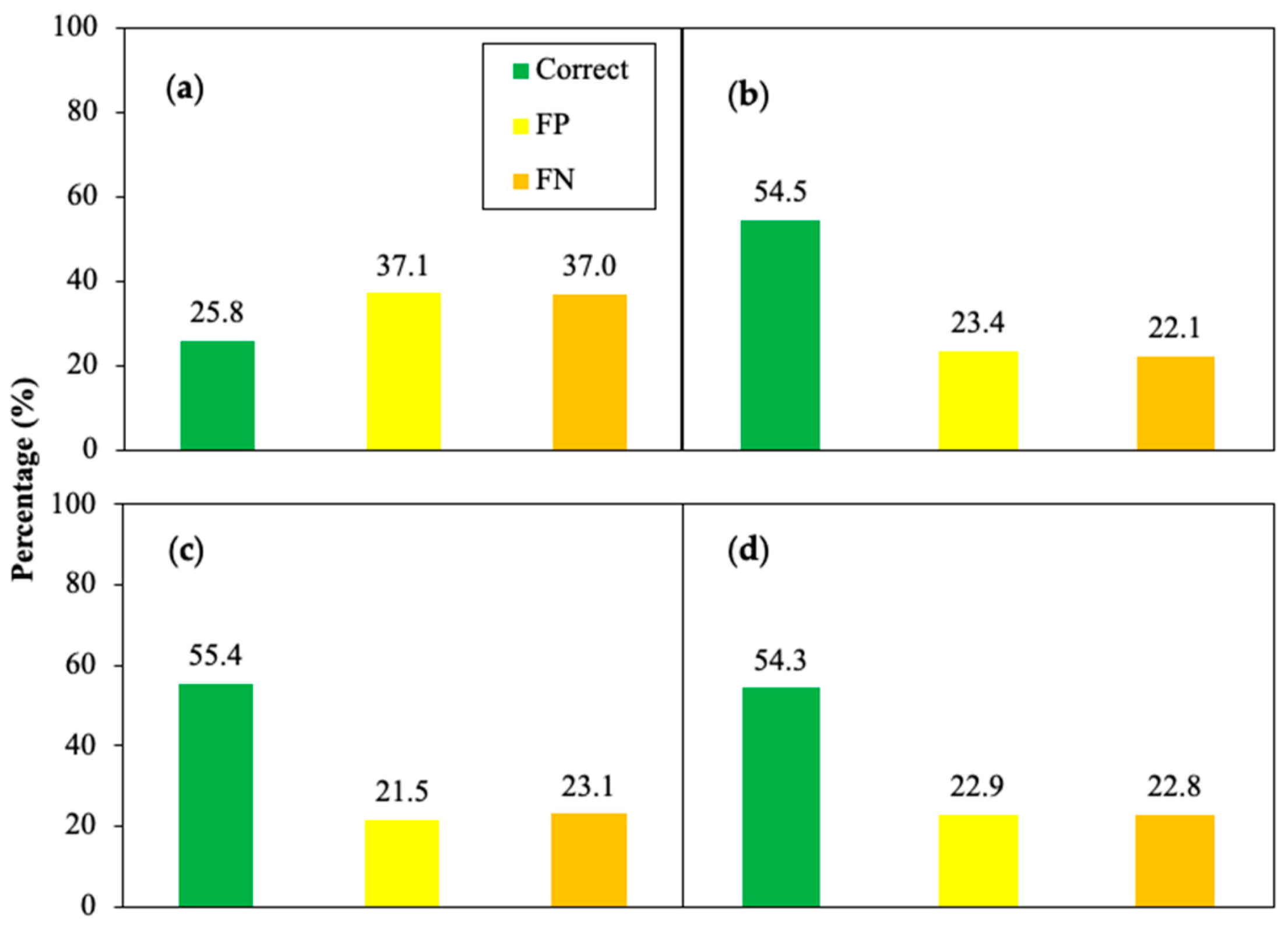
3.3. Impacts of DEM Resolution on Prediction Accuracy

The accuracies of riparian zone prediction using optimal parameters specific to each DEM are shown in Figure 9. As mentioned, KC for coarse resolution DEM was 0.25, which is remarkably lower than the KC of 0.64 and 0.63 achieved by high-resolution DEMs. These results indicated a substantial improvement with high-resolution DEMs (LiDAR and UAV) compared with traditional coarse resolution DEM for delineation of riparian zones. We also found the riparian zone prediction accuracies using high-resolution DEMs did not have significant differences, and the KC results were practically identical (0.63 and 0.64). The percentage area of the field-surveyed riparian zone being classified as upland using the three DEMs were 22.1%, 23.1%, and 22.8% for LiDAR1.2, LiDAR6.0, and UAV DEM, respectively (Figure 9), which reflected nearly identical performance.
Field-surveyed riparian zones together with predicted riparian zones with different DEMs are shown in Figure 10. With traditional coarse resolution DEM, large discrepancies between predicted and field-surveyed riparian zones were found over a large part of the north section of the study site (Figure 10a). Nonetheless, this area was correctly classified as a riparian zone by all higher resolution DEM including LiDAR or UAV.
On the eastern side of the stream, riparian zones predicted by DEM were substantially larger than the field-surveyed mapped riparian zones (Figure 10). However, the riparian zone boundary predicted by UAV and LiDAR 6.0-derived DEMs appeared to better match the field-surveyed riparian zone boundaries compared with LiDAR 1.2. The riparian zone predicted by LiDAR1.2 tended to join the two functional riparian areas located on the eastern side of the stream together (where the higher discrepancy was detected). This must have been due to the higher capability of the UAV and LiDAR 6.0 of detecting the microtopography compared with LiDAR 1.2 and divided the first two wet areas mentioned more clearly. Additionally, due to this higher resolution, the LiDAR 6.0 and UAV-derived DEM identified seasonal stream paths more accurately and therefore represented a wider stream network.
We also found that all DEMs misclassified the riparian zone in the section where the stream was partially restored (bioengineered buffer), located beside the planted forest where the road divides these two areas, along the southern half part of the map (Figure 10).

4. Discussion

4.1. Impact of the DEM Resolution

We observed significant differences between the accuracy achieved with the traditional coarse resolution DEM compared with higher resolution DEMs. Previous studies also reported that coarse resolution DEMs could not adequately represent the topographic features due to greater terrain surface generalizations [22,44,53,54]. This research confirmed that traditional coarse resolution DEMs could not be used for riparian zone delineation in low-order streams. With their higher elevation point density and higher vertical accuracy, higher resolution DEMs derived by LiDAR and UAV can represent the subtle elevation changes in microtopography in greater detail. Previous researchers also pointed out that higher quality vertical information resulted in appreciable improvements in the representation of topographic surface details [55,56,57,58,59]. Higher resolution and accuracy also provided more accurate delineations of hydrologically relevant parameters and more appropriate model outputs [55,56,57,58,59]. This can ultimately explain the differences in the VDTCN thresholds used between low resolution and high-resolution DEMs.

4.2. VDTCN Raster Performance in Each DEM

Analysis of results highlighted slight differences between the three high-resolution DEMs used in this study. Overall, LiDAR 1.2 displayed a more general stream network grid, whereas the LiDAR 6.0 and UAV provided a more complex detail. Consequently, relatively shallower areas became less constrained using LiDAR 1.2-derived DEM. This seems to be the reason for the slightly lower correctness achieved compared to using UAV and LiDAR 6.0. These results seem to contradict the concept concluded by previous studies in which smoother topography represented in “coarser” resolutions would reduce the confounding effects of microtopography and increase correctness [54,60,61,62]. These studies reported that a more general topography of the landscape represented subsurface groundwater level (GWL) flow paths more accurately than a 1 m DEM.
We found that all three high-resolution DEMs performed poorly in two specific areas. The first area was located within the bioengineered buffer. In this area, a large portion of the riparian area was classified as upland. This section was fenced off and eliminated access by cattle as part of riparian zone conservation. In addition to high vegetation, the herbaceous species were also dense and tall, even during the spring. We suspected that LiDAR might not distinguish the ground surface from the grass cover, so we, therefore, captured the UAV images in early spring. However, the snow-flattened grass formed a surface that was substantially higher than bare ground and caused DEM discrepancies (Figure 11). These results indicated that both UAV and LiDAR had successfully isolated the presence of trees but could not distinguish the denser grass. In a future study, landmarks could be set up to estimate grass height manually in order to improve the delineation accuracy.
The second area of discrepancy was found close to the trail created by cattle traveling along a fenced area over the pasture (Figure 11). In this section, a large area was predicted to be a riparian zone but was not classified as riparian in the field surveys. We considered that this area actually should be classified as a riparian zone, but grazing by cattle has removed all riparian vegetation, making it difficult to identify. Therefore, this prediction should not be considered as an error, but the area was a disturbed riparian area.

5. Conclusions

In this study, we aimed to assess the precision of predicting the extent of the functional riparian zones on a farm to further improve the detection of hydrologically sensitive areas and critical source areas in farmland with similar characteristics, land use, and topography in southeastern New Brunswick (Canada). To do so, we compared the efficiency of the VDTCN classifying this ecotone when using different topographical models as a source: coarse mass points DEM, obtained with traditional photogrammetry, LiDAR at different resolutions (1.2 and 6 point m−2), and the UAV-derived DEM.
The most noticeable differences were found between the low and high-resolution DEMs (traditional DEM vs. LiDAR and UAV DEMs). The traditional coarse resolution DEM performed poorly in classifying functional riparian zones with KC as low as 0.25 compared with KC = 0.63–0.64 for high-resolution DEMs by LiDAR and UAV. We also found that direct use of optimal parameters (minimal flow initiation threshold and VDTCN threshold) for the coarse resolution DEM to high-resolution DEMs could lead to large errors.
We found that UAV-derived DEM could be used to delineate riparian zones using VDTCN as a classifier for lower-order streams, with comparable accuracy to that of airborne high point cloud density LiDAR. However, tall grassed areas could cause misclassification using LiDAR or UAV methods.

Author Contributions

Conceptualization, J.G. and K.L.; methodology, J.G. and F.-R.M.; software, J.O.; validation, J.G., F.-R.M., and P.A.; formal analysis, S.L.; investigation, J.G.; resources, B.R.; data curation, F.-R.M.; writing—original draft preparation, J.G.; writing—review and editing, B.R.; visualization, F.-R.M.; supervision, F.-R.M.; project administration, B.R.; funding acquisition, B.R. All authors have read and agreed to the published version of the manuscript.

Funding

Please add: This research was funded by Agriculture and Agri-food Canada (AAFC).

Acknowledgments

This study was funded by Agriculture and Agri-Food Canada. The first author is grateful for the financial support provided by the Fredericton Research and Development Centre (FRDC) in New Brunswick. Special thanks are given to Louis-Pierre Comeau, Rebecca Hersom-Petersen, Amalia David, and Robert Hicks, farm crews, and summer student Madisyn Harper for their dedicated field/lab assistance.

Conflicts of Interest

The authors declare no conflict of interest.

References

  1. Hill, A.R.; Cardaci, M. Denitrification and organic carbon availability in riparian wetland soils and subsurface sediments. Soil Sci. Soc. Am. J. 2004, 68, 320–325. [Google Scholar] [CrossRef]
  2. Naiman, R.J.; Decamps, H. The ecology of interfaces: Riparian zones. Annu. Rev. Ecol. Syst. 1997, 28, 621–658. [Google Scholar] [CrossRef] [Green Version]
  3. Swanson, S.; Miles, R.; Leonard, S.; Genz, K. Classifying rangeland riparian areas: The Nevada task force approach. J. Soil Water Conserv. 1988, 43, 259–263. [Google Scholar]
  4. Cooper, J.; Gilliam, J.; Daniels, R.; Robarge, W. Riparian areas as filters for agricultural sediment. Soil Sci. Soc. Am. J. 1987, 51, 416–420. [Google Scholar] [CrossRef]
  5. Meehan, W.R.; Swanson, F.J.; Sedell, J.R. Influences of riparian vegetation on aquatic ecosystems with particular reference to salmonid fishes and their food supply. In Proceedings of the Importance, Preservation and Management of Riparian Habitat: A Symposium, Tucson, Arizona, 9 July 1977; p. 137. [Google Scholar]
  6. Peterson, B.J.; Wollheim, W.M.; Mulholland, P.J.; Webster, J.R.; Meyer, J.L.; Tank, J.L.; Martí, E.; Bowden, W.B.; Valett, H.M.; Hershey, A.E. Control of nitrogen export from watersheds by headwater streams. Science 2001, 292, 86–90. [Google Scholar] [CrossRef]
  7. Swanson, F.; Gregory, S.; Sedell, J.; Campbell, A. Land-Water Interactions: The Riparian Zone. 1982. Available online: https://www.researchgate.net/publication/265105931_9_Land-Water_Interactions_The_Riparian_Zone (accessed on 1 April 2021).
  8. Likens, G.E. Lake Ecosystem Ecology: A Global Perspective; Academic Press: Cambridge, MA, USA, 2010. [Google Scholar]
  9. Sedell, J.R.; Beschta, R.L. Bringing Back the ’Bio’ in Bioengineering. In Fisheries Bioengineering Symposium: American Fisheries Society Symposium 10; American Fisheries Society: Bethesda, MD, USA, 1991; p. 160. [Google Scholar]
  10. Johansen, K.; Phinn, S.; Dixon, I.; Douglas, M.; Lowry, J. Comparison of image and rapid field assessments of riparian zone condition in Australian tropical savannas. For. Ecol. Manag. 2007, 240, 42–60. [Google Scholar] [CrossRef]
  11. Rivenbark, B.L.; Jackson, C.R. Concentrated flow breakthroughs moving through silvicultural streamside management zones: Southeastern piedmont, USA 1. JAWRA J. Am. Water Resour. Assoc. 2004, 40, 1043–1052. [Google Scholar] [CrossRef]
  12. Werren, G.; Arthington, A. The assessment of riparian vegetation as an indicator of stream condition, with particular emphasis on the rapid assessment of flow-related impacts. In Landscape Health of Queensland; Royal Society of Queenland: Brisbane, Australia, 2002; pp. 194–222. [Google Scholar]
  13. Fu, B.; Li, Y.; Wang, Y.; Campbell, A.; Zhang, B.; Yin, S.; Zhu, H.; Xing, Z.; Jin, X. Evaluation of riparian condition of Songhua River by integration of remote sensing and field measurements. Sci. Rep. 2017, 7, 2565. [Google Scholar] [CrossRef] [Green Version]
  14. Congalton, R.G.; Birch, K.; Jones, R.; Schriever, J. Evaluating remotely sensed techniques for mapping riparian vegetation. Comput. Electron. Agric. 2002, 37, 113–126. [Google Scholar] [CrossRef]
  15. Johansen, K.; Phinn, S. Mapping structural parameters and species composition of riparian vegetation using IKONOS and Landsat ETM+ data in Australian tropical savannahs. Photogramm. Eng. Remote Sens. 2006, 72, 71–80. [Google Scholar] [CrossRef]
  16. Chaplot, V.; Walter, C.; Curmi, P. Improving soil hydromorphy prediction according to DEM resolution and available pedological data. Geoderma 2000, 97, 405–422. [Google Scholar] [CrossRef]
  17. Ilhardt, B.L.; Verry, E.S.; Palik, B.J. Defining riparian areas. For. Riparian Zone Orono Maine 2000, 26, 7–14. [Google Scholar]
  18. Abood, S.A.; Maclean, A.L.; Mason, L.A. Modeling riparian zones utilizing DEMS and flood height data. Photogramm. Eng. Remote Sens. 2012, 78, 259–269. [Google Scholar] [CrossRef]
  19. Gallant, J.C.; Dowling, T.I. A multiresolution index of valley bottom flatness for mapping depositional areas. Water Resour. Res. 2003, 39. [Google Scholar] [CrossRef]
  20. Murphy, P.; Ogilvie, J.; Arp, P. Topographic modelling of soil moisture conditions: A comparison and verification of two models. Eur. J. Soil Sci. 2009, 60, 94–109. [Google Scholar] [CrossRef]
  21. Johansen, K.; Grove, J.; Denham, R.; Phinn, S.R. Assessing stream bank condition using airborne LiDAR and high spatial resolution image data in temperate semirural areas in Victoria, Australia. J. Appl. Remote Sens. 2013, 7, 073492. [Google Scholar] [CrossRef] [Green Version]
  22. Vaze, J.; Teng, J.; Spencer, G. Impact of DEM accuracy and resolution on topographic indices. Environ. Model. Softw. 2010, 25, 1086–1098. [Google Scholar] [CrossRef]
  23. Holmes, K.L.; Goebel, P.C.; Morris, A.E. Characteristics of downed wood across headwater riparian ecotones: Integrating the stream with the riparian area. Can. J. For. Res. 2010, 40, 1604–1614. [Google Scholar] [CrossRef]
  24. Smith, M.P.; Schiff, R.; Olivero, A.; MacBroom, J. The Active River Area: A Conservation Framework for Protecting Rivers and Streams; The Nature Conservancy: Boston, MA, USA, 2008. [Google Scholar]
  25. Buchanan, B.; Fleming, M.; Schneider, R.; Richards, B.; Archibald, J.; Qiu, Z.; Walter, M. Evaluating topographic wetness indices across central New York agricultural landscapes. Hydrol. Earth Syst. Sci. 2014, 18, 3279–3299. [Google Scholar] [CrossRef] [Green Version]
  26. Bock, M.; Köthe, R. Predicting the depth of hydromorphic soil characteristics influenced by ground water. SAGA Second. Out 2008, 19, 13–22. [Google Scholar]
  27. Kokulan, V.; Akinremi, O.; Moulin, A.P.; Kumaragamage, D. Importance of terrain attributes in relation to the spatial distribution of soil properties at the micro scale: A case study. Can. J. Soil Sci. 2018, 98, 292–305. [Google Scholar] [CrossRef] [Green Version]
  28. Malone, B.P.; Odgers, N.P.; Stockmann, U.; Minasny, B.; McBratney, A.B. Digital mapping of soil classes and continuous soil properties. In Pedometrics; Springer: Berlin/Heidelberg, Germany, 2018; pp. 373–413. [Google Scholar]
  29. Carrivick, J.L.; Smith, M.W.; Quincey, D.J.; Carver, S.J. Developments in budget remote sensing for the geosciences. Geol. Today 2013, 29, 138–143. [Google Scholar] [CrossRef]
  30. Villanueva, J.R.E.; Martínez, L.I.; Montiel, J.I.P. DEM generation from fixed-wing UAV imaging and LiDAR-derived ground control points for flood estimations. Sensors 2019, 19, 3205. [Google Scholar] [CrossRef] [Green Version]
  31. Fonstad, M.A.; Dietrich, J.T.; Courville, B.C.; Jensen, J.L.; Carbonneau, P.E. Topographic structure from motion: A new development in photogrammetric measurement. Earth Surf. Process. Landf. 2013, 38, 421–430. [Google Scholar] [CrossRef] [Green Version]
  32. Jeziorska, J. UAS for wetland mapping and hydrological modeling. Remote Sens. 2019, 11, 1997. [Google Scholar] [CrossRef] [Green Version]
  33. Rahman, M.M.; McDermid, G.J.; Strack, M.; Lovitt, J. A new method to map groundwater table in peatlands using unmanned aerial vehicles. Remote Sens. 2017, 9, 1057. [Google Scholar] [CrossRef] [Green Version]
  34. Shamshiri, R.R.; Hameed, I.A.; Balasundram, S.K.; Ahmad, D.; Weltzien, C.; Yamin, M. Fundamental research on unmanned aerial vehicles to support precision agriculture in oil palm plantations. Agric. Robot. Fundam. Appl. 2018, 6, 91–116. [Google Scholar]
  35. Kuželka, K.; Surový, P. Mapping forest structure using UAS inside flight capabilities. Sensors 2018, 18, 2245. [Google Scholar] [CrossRef] [Green Version]
  36. Krisanski, S.; Taskhiri, M.S.; Turner, P. Enhancing methods for under-canopy unmanned aircraft system based photogrammetry in complex forests for tree diameter measurement. Remote Sens. 2020, 12, 1652. [Google Scholar] [CrossRef]
  37. Rogers, S.R.; Manning, I.; Livingstone, W. Comparing the spatial accuracy of Digital Surface Models from four unoccupied aerial systems: Photogrammetry versus LiDAR. Remote Sens. 2020, 12, 2806. [Google Scholar] [CrossRef]
  38. White, B.; Ogilvie, J.; Campbell, D.M.; Hiltz, D.; Gauthier, B.; Chisholm, H.K.H.; Wen, H.K.; Murphy, P.N.; Arp, P.A. Using the cartographic depth-to-water index to locate small streams and associated wet areas across landscapes. Can. Water Resour. J. Rev. Can. Ressour. Hydr. 2012, 37, 333–347. [Google Scholar] [CrossRef]
  39. Elmore, A.J.; Julian, J.P.; Guinn, S.M.; Fitzpatrick, M.C. Potential stream density in Mid-Atlantic US watersheds. PLoS ONE 2013, 8, e74819. [Google Scholar] [CrossRef] [Green Version]
  40. Wolf, R.; Dewitt, A. Elements of Photogrammetry with Application in GIS, 3rd ed.; The University of Wisconsin: Madison, WI, USA, 2000. [Google Scholar]
  41. Beni, L.H.; Jones, J.; Thompson, G.; Johnson, C.; Gebrehiwot, A. Challenges and Opportunities for UAV-Based Digital Elevation Model Generation for Flood-Risk Management: A Case of Princeville, North Carolina. Sensors 2018, 18, 3843. [Google Scholar] [CrossRef] [Green Version]
  42. Poppenga, S.K.; Worstell, B.B.; Stoker, J.M.; Greenlee, S.K. Using Selective Drainage Methods to Extract Continuous Surface Flow from 1-Meter Lidar-Derived Digital Elevation Data; U. S. Geological Survey: Reston, VA, USA, 2010.
  43. Zhang, W.; Montgomery, D.R. Digital elevation model grid size, landscape representation, and hydrologic simulations. Water Resour. Res. 1994, 30, 1019–1028. [Google Scholar] [CrossRef]
  44. Hancock, G.R. The use of digital elevation models in the identification and characterization of catchments over different grid scales. Hydrol. Process. Int. J. 2005, 19, 1727–1749. [Google Scholar] [CrossRef]
  45. O’Callaghan, J.F.; Mark, D.M. The extraction of drainage networks from digital elevation data. Comput. Vis. Graph. Image Process. 1984, 28, 323–344. [Google Scholar] [CrossRef]
  46. Brander, L.; Schuyt, K. The Economic Values of the World’s Wetlands. 2004. Available online: https://www.cbd.int/financial/values/g-value-wetlands.pdf (accessed on 1 April 2021).
  47. Wilson, A.M.; Evans, T.; Moore, W.; Schutte, C.A.; Joye, S.B.; Hughes, A.H.; Anderson, J.L. Groundwater controls ecological zonation of salt marsh macrophytes. Ecology 2015, 96, 840–849. [Google Scholar] [CrossRef]
  48. Londo, G. The decimal scale for releves of permanent quadrats. Vegetatio 1976, 33, 61–64. [Google Scholar] [CrossRef]
  49. Bouma, J.T. Hydrology and soil genesis of soils with aquic moisture regimes. In Pedogenesis and Soil Taxonomy; Wilding, L.P., Smeck, N.E., Hall, G.F., Eds.; Elsevier: Amsterdam, The Netherlands, 1983. [Google Scholar]
  50. Jacobs, P.M.; West, L.T.; Shaw, J.N. Redoximorphic features as indicators of seasonal saturation, Lowndes County, Georgia. Soil Sci. Soc. Am. J. 2002, 66, 315–323. [Google Scholar] [CrossRef]
  51. Congalton, R.G.; Mead, R.A. A quantitative method to test for consistency and correctness in photointerpretation. Photogramm. Eng. Remote Sens. 1983, 49, 69–74. [Google Scholar]
  52. Fabian, A.J.; Klenke, R.; Truslow, P. Improving UAV-Based Target Geolocation Accuracy through Automatic Camera Parameter Discovery. In AIAA Scitech 2020 Forum; American Institute of Aeronautics and Astronautics: Reston, VA, USA, 2020; p. 2201. [Google Scholar]
  53. Chang, K.-T.; Tsai, B.-W. The effect of DEM resolution on slope and aspect mapping. Cartogr. Geogr. Inf. Syst. 1991, 18, 69–77. [Google Scholar] [CrossRef]
  54. Thompson, J.A.; Bell, J.C.; Butler, C.A. Digital elevation model resolution: Effects on terrain attribute calculation and quantitative soil-landscape modeling. Geoderma 2001, 100, 67–89. [Google Scholar] [CrossRef]
  55. Eltner, A.; Kaiser, A.; Castillo, C.; Rock, G.; Neugirg, F.; Abellán, A. Image-based surface reconstruction in geomorphometry–merits, limits and developments. Earth Surf. Dyn. 2016, 4, 359–389. [Google Scholar] [CrossRef] [Green Version]
  56. Grabs, T.; Seibert, J.; Bishop, K.; Laudon, H. Modeling spatial patterns of saturated areas: A comparison of the topographic wetness index and a dynamic distributed model. J. Hydrol. 2009, 373, 15–23. [Google Scholar] [CrossRef] [Green Version]
  57. Nobre, A.D.; Cuartas, L.A.; Hodnett, M.; Rennó, C.D.; Rodrigues, G.; Silveira, A.; Saleska, S. Height Above the Nearest Drainage–a hydrologically relevant new terrain model. J. Hydrol. 2011, 404, 13–29. [Google Scholar] [CrossRef] [Green Version]
  58. Schmid, K.A.; Hadley, B.C.; Wijekoon, N. Vertical accuracy and use of topographic LIDAR data in coastal marshes. J. Coast. Res. 2011, 27, 116–132. [Google Scholar] [CrossRef]
  59. Sonneveld, M.; Schoorl, J.; Veldkamp, A. Mapping hydrological pathways of phosphorus transfer in apparently homogeneous landscapes using a high-resolution DEM. Geoderma 2006, 133, 32–42. [Google Scholar] [CrossRef]
  60. Gillin, C.P.; Bailey, S.W.; McGuire, K.J.; Prisley, S.P. Evaluation of LiDAR-derived DEMs through terrain analysis and field comparison. Photogramm. Eng. Remote Sens. 2015, 81, 387–396. [Google Scholar] [CrossRef] [Green Version]
  61. Sørensen, R.; Seibert, J. Effects of DEM resolution on the calculation of topographical indices: TWI and its components. J. Hydrol. 2007, 347, 79–89. [Google Scholar] [CrossRef]
  62. Wolock, D.M.; Price, C.V. Effects of digital elevation model map scale and data resolution on a topography-based watershed model. Water Resour. Res. 1994, 30, 3041–3052. [Google Scholar] [CrossRef]
Figure 1. Location of study area (Hicksville settlement, Havelock, NB); (a) The Ridge Brook subcatchment; (b) the location of the watershed in New Brunswick; (c) the location of the study area within the watershed. The red rectangle in (c) covers the bioengineered buffer area. The star point is the area affected by intense cattle grazing and cattle resting. The stream follows South to North direction.
Remotesensing 13 01997 g001
Figure 2. The DJI Phantom 4 Pro set up in the field.
Remotesensing 13 01997 g002
Figure 3. Distribution of the GCPs in the study area.
Remotesensing 13 01997 g003
Figure 4. Flowchart of the methodology for delineating functional riparian zones and flow paths.
Remotesensing 13 01997 g004
Figure 5. Interpolated DEMs with point clouds from different data sources: (a) coarse resolution (“burn” DEM); (b) LiDAR 1.2; (c) LiDAR 6.0; (d) UAV. Elevation values are displayed in meters. The difference in the lowest value registered in (a) is due to imprinting field-mapped open drainage channel network to create the “burn” DEM.
Remotesensing 13 01997 g005
Figure 6. Stream network (Top Panels) and VDTCN (Lower Panels) with different minimum flow initiation thresholds using the coarse resolution DEM as a source: (a,d) 0.5 hectares; (b,e) 1 hectare; (c,f) 1.5 hectares. The different colors represent different VDTCN thresholds, expressed in meters.
Remotesensing 13 01997 g006
Figure 7. UAV images obtained in (a) Spring, (b) late Summer, and (c) Fall. As can be seen, (a) displays better detail of wet areas. The numbers in (a) represent the different functional riparian areas measured in the field.
Remotesensing 13 01997 g007
Figure 8. The VDTCN maps derived from different high-resolution DEMs using different flow initiation thresholds; from left to right, minimum flow initiation: 0.5 hectares; 1.0 and 1.5 ha, respectively. Figures (ac) show the VDTCN using the LIDAR1.2 as a source. Figures (df) show the VDTCN using the LiDAR 6.0 as a source. Figures (gi) show the VDTCN thresholds using the UAV-derived DEM as a source.
Remotesensing 13 01997 g008
Figure 9. Accuracy of the VDTCN predicted functional riparian zones using different DEMs and optimal parameters: (a) mass points coarse resolution DEM, flow initiation = 1.5 ha, VDTCN threshold = 14.2 m; (b) LiDAR 1.2, flow initiation = 0.75 ha, VDTCN threshold = 0.40 m; (c) LiDAR 6.0, flow initiation = 0.75 ha, VDTCN threshold = 0.48 m; (d) UAV DEM, flow initiation = 0.5 ha, VDTCN threshold = 0.48 m. (FP = false positive, indicates upland being predicted as riparian zone; FN = false negative, indicates riparian zone being misclassified as upland).
Remotesensing 13 01997 g009
Figure 10. Optimal results for the functional riparian zone predicted by the VDTCN raster using each DEM as a source: (a) coarse mass points; (b) LiDAR 1.2p m−2, (c) LiDAR 6.0p m−2, and (d) UAV.
Remotesensing 13 01997 g010
Figure 11. Study area showing the two areas of discrepancy. On the left, the stream capture corresponding to summer when LiDAR was collected. On the right, the cattle grazing and trampling beside the fence mentioned (the boundary between grass and grazed area).
Remotesensing 13 01997 g011
Table 1. Accuracy of riparian zone prediction with different DEM and different Flow Initiation (FI) and VDTCN thresholds. Results for the VDTCN raster using different DEMs and different Flow initiation (F. I.). (DEM LiDAR1.2 = LiDAR with a density of 1.2 points m−2; LiDAR6.0 = LiDAR with a density of 6 points m−2).
DEMInterpolationF. I.
(ha)
VDTCN Threshold (m)Overall
Accuracy (%)
Kappa
Coefficient
Coarse2 m1.514.2750.25
LiDAR 1.230 cm1.514.2270.04
LiDAR 6.030 cm1.514.2260.03
UAV30 cm1.514.2260.03
LiDAR 1.230 cm0.750.40880.63
LiDAR 6.030 cm0.750.40890.63
UAV30 cm0.750.40880.56
LiDAR 6.030 cm0.750.48880.64
UAV30 cm0.750.48870.59
UAV30 cm0.50.48880.63
Publisher’s Note: MDPI stays neutral with regard to jurisdictional claims in published maps and institutional affiliations.

