
Regularized CNN Feature Hierarchy for Hyperspectral Image Classification


1
Department of Computer Science, Chiniot-Faisalabad Campus, National University of Computer and Emerging Sciences, Islamabad, Chiniot 35400, Pakistan
2
Dipartimento di Matematica e Informatica-MIFT, University of Messina, 98121 Messina, Italy
3
Institute of Software Development and Engineering, Innopolis University, 420500 Innopolis, Russia
*
Author to whom correspondence should be addressed.
Remote Sens. 2021, 13(12), 2275; https://doi.org/10.3390/rs13122275
Submission received: 28 April 2021
/
Revised: 2 June 2021
/
Accepted: 7 June 2021
/
Published: 10 June 2021
(This article belongs to the Special Issue Hyperspectral Remote Sensing: Current Situation and New Challenges)
Abstract
:Convolutional Neural Networks (CNN) have been rigorously studied for Hyperspectral Image Classification (HSIC) and are known to be effective in exploiting joint spatial-spectral information with the expense of lower generalization performance and learning speed due to the hard labels and non-uniform distribution over labels. Therefore, this paper proposed an idea to enhance the generalization performance of CNN for HSIC using soft labels that are a weighted average of the hard labels and uniform distribution over ground labels. The proposed method helps to prevent CNN from becoming over-confident. We empirically show that, in improving generalization performance, regularization also improves model calibration, which significantly improves beam-search. Several publicly available Hyperspectral datasets are used to validate the experimental evaluation, which reveals improved performance as compared to the state-of-the-art models with overall 99.29%, 99.97%, and 100.0% accuracy for Indiana Pines, Pavia University, and Salinas dataset, respectively.
1. Introduction
Hyperspectral Imaging (HSI) has been extensively utilized for many real-world applications [1]—for instance, crop monitoring [2], vegetation coverage [3], precision agriculture [4], land resources [5], oil spills [6], water quality [7], meat adulteration [8,9], adulteration in household products such as color adulteration in red chili [10,11], microbial spoilage, and shelf-life of bakery products [12].
Thus, HSI Classification (HSIC) has received remarkable attention and intensive research results have been reported in the past few decades [13]. According to the literature, HSIC can be categorized into spatial, spectral, and spatial-spectral feature methods [14]. The spectral feature can be labeled as a primitive characteristic of HSI also known as spectral curve or vector, whereas the spatial feature contains the relationship between the central pixel and its context, which significantly improves the performance [15].
In the last few years, deep learning, especially Convolutional Neural Networks (CNNs), has received widespread attention due to its ability to automatically learn nonlinear features for classification, i.e., overcome the challenges of hand-crafted features for HSIC using traditional methods [16] such as Support Vector Machine (SVM), K-Nearest Neighbor (KNN), Random Forest, Ensemble Learning, Artificial Neural Network, and Extreme Learning Machine (ELM) [17,18]. Moreover, CNN can jointly investigate the spatial-spectral information and such models can be categorized into two groups, i.e., single and two-stream; more information regarding single or two-stream methods can be found in [19]. This work explicitly investigates a single-stream method similar to the works proposed by Ahmad et al. [20] (A Fast and Compact 3D CNN for HSIC), Xie et al. [21] (Hyperspectral Face Recognition-based on Sparse Spectral Attention Deep Neural Network), Liu et al. [22] (A semi-supervised CNN for HSIC), Hamida et al. [23] (3D Deep Learning Approach for Remote Sensing Image Classification), Lee et al. [24] (Contextual Deep CNN-based HSIC), Chen et al. [25] (Contextual Deep CNN-based HSIC), Li [26] (Spectral–Spatial Classification of HSI with 3D CNN), He et al. [27] (Multi-scale 3D Deep CNN Network for HSI), Zhao et al. [28] (Hybrid Depth-Separable Residual Networks for HSIC). Yang et al. [29] (Synergistic 2D/3D CNN for HSIC).
Irrespective of the single or two-stream methods, all deep learning frameworks discussed above are sensitive to the loss, which needs to be minimized [30]. Several classical works showed that the gradient descent to minimize cross-entropy performs better in terms of classification and has fast convergence; however, to some extent, this leads to the overfitting [31]. Several regularization techniques, such as dropout [32], L1, L2 [33], etc., have been used to overcome the overfitting issues together with several other exotic objectives performed exceptionally well compared to the standard cross-entropy [34]. Recently, a work [35] proposed a regularization technique that improves the accuracy significantly by computing cross-entropy with a weighted mixture of targets with uniform distribution instead of hard-coded targets.
Since then, regularization has been known to improve the classification performance of deep models [36]. However, the original idea was used to improve the classification performance of only the inception model on ImageNet data [35]. Despite this, various image classification models have used regularization [37,38]. Though the regularization technique is a widely used trick to improve the classification performance and to speed up the convergence process, it has not been much explored for HSIC, and, above all, regarding when and why regularization should work have not been explored very much.
Considering the aforementioned issues, this paper proposed a novel idea to enhance the generalization performance of CNN for HSIC using soft labels that are a weighted average of the hard labels and uniform distribution over target labels. The proposed method helps to prevent CNN from becoming over-confident. We empirically show that, in improving generalization performance, regularization also improves model calibration, which significantly improves beam-search. Several publicly available Hyperspectral datasets are used to validate the experimental evaluation, which reveals improved generalization performance, statistical significance, and computational complexity as compared to the state-of-the-art 2D/3D CNN models.
2. Problem Formulation
Let us assume that the Hyperspectral data can be represented as , where is the total number of bands. are the samples per band belonging to Y classes and is the sample in the Hyperspectral Data. Suppose , where is the class label of the sample. For HSI classification with Y candidate labels, for example, lets assume , where is the class label of the sample belonging to the training set and the ground truth distribution p over labels and . One can have a model with parameters that predicts the predicted label distribution as and, of course, . Thus, the cross entropy in this particular case would be .
If one have instance in the training set, then the loss function would be which can further modify as . However, in nature, the would be a one-hot-encoded vector [14,39], which can be defined as:
Based on the above objective, one can reduce the loss function as . Minimizing L is equivalent to conduct maximum likelihood estimation over the training set. However, during optimisation, it is possible to minimize L to almost 0, if, and only if, all the instances in the dataset do not have conflicting labels (Conflicting labels means that there are two examples with the same features but their ground truths are different.) This is due to being computed from soft-max as:
where is the logit for candidate class i. The consequence of using one-hot-encoding is that will be extremely large and where will be extremely small. Given a non-conflicting dataset, the ultimate model will classify every training instance correctly with the confidence of almost 1. This is certainly a signature of overfitting, and the overfitted model does not generalize well. Thus, this work used a regularization technique (noise distribution) irrespective to traditional techniques proposed in literature [40,41,42] for deep models [43]. Thus, the new HSI ground truths would be:
where is a weight factor, and note that . These new ground truths have been used in loss function instead of one-hot-encoding [44]:
where is the loss function, and is the estimated probabilities. It can be argued that, for each ground truth, the loss contribution is a mixture of entropy between predicted distribution () and the one-hot-encoding, and the entropy between the predicted distribution () and the noise distribution. While training, if the model learns to predict the distribution confidently; however, will increase dramatically. To overcome this phenomenon, we used a regularizer to prevent the model from predicting too confidently. In practice, is a uniform distribution that does not depend on hyperspectral data. That is to say, .
3. Experimental Settings and Results
The experiments have been conducted on three real HSI datasets, namely, Indian Pines (IP), Salinas full scene, and Pavia University (PU). These datasets are acquired by two different sensors. i.e., Reflective Optics System Imaging Spectrometer (ROSIS) and Airborne Visible/Infrared Imaging Spectrometer (AVIRIS) [13]. The experimental results explained in this work have been obtained through Google Colab [45], an online platform to execute any Python environment even on Graphical Processing Unit (GPU), providing up to 358+ GB of cloud storage, and 25 GB of Random Access Memory (RAM).
In all the experiments, the initial size of the train/validation/test sets is set to 25%/25%/50% to validate the proposed model as well as several other state-of-the-art deep models. Five models have been used as baseline for the experiments: AlexNet, LeNet, 2D CNN, 3D CNN, and a Hybrid (3D/2D) CNN model. The details of the above-mentioned model are as follows.
- (1)
- The AlexNet model consists of five convolutional layers with 96, 256, 384, 384, 256 filters, while each layer has , , , , and filter sizes. One pooling layer after the first convolutional layer. A flattened layer, dense layers with 4096 units. After each dense layer, a dropout layer has been used with 0.5%. Finally, an output layer has been used with the total number of classes to predict [46].
- (2)
- The LeNet model has two convolutional layers in which each layer has 32 and 64 filters with and filter sizes, respectively. One pooling layer after first convolutional layer, a flattened layer, dense layer with 100 units. Finally, an output layer has been used with the total number of classes to predict [47].
- (3)
- The 2D CNN model is composed of four convolutional layers in which each layer has 8, 16, 32, and 64 filters with filter size. A flattened layer, two dense layers with 256 and 100 units, and, after each dense layer, a dropout layer has been used with 0.4%. Finally, an output layer has been used with the total number of classes to predict [32].
- (4)
- The 3D CNN is composed of four convolutional layers in which each layer has 8, 16, 32, and 64 filters with , , , and filter sizes. A flattened layer, two dense layers with 256 and 128 units, and, after each dense layer, a dropout layer has been used with 0.4%. Finally, an output layer has been used with the total number of classes to predict [20].
- (5)
- The details of hybrid (3D/2D) convolutional layers and kernels are as follows: 3D conv layer 1 i.e., and . 3D conv layer 2 i.e., . . 3D conv layer 3 i.e., and . 3D conv layer 4 i.e., and . 3D conv layer 5 i.e., and . Three 3D convolutional layers are employed to increase the number of spectral-spatial feature maps, and one 2D convolutional layer is used to discriminate the spatial features within different spectral bands while preserving the spectral information.
Initially, the weights are randomized and then optimized using back-propagation with the Adam optimizer by using the loss function presented in Equation (8). Further details regarding the CNN architectures in terms of types of layers, dimensions of output feature maps and number of trainable parameters can be found in [13,20,32,46,47].
In order to validate the claims made in this manuscript, the following accuracy metrics have been assessed. They include: Kappa ( is known as a statistical metric that considered the mutual information regarding a strong agreement among classification and ground-truth maps), average (AA represents the average class-wise classification performance), and overall (OA is computed as the number of correctly classified examples out of the total test examples). Such metrics are computed using the following equations:
where
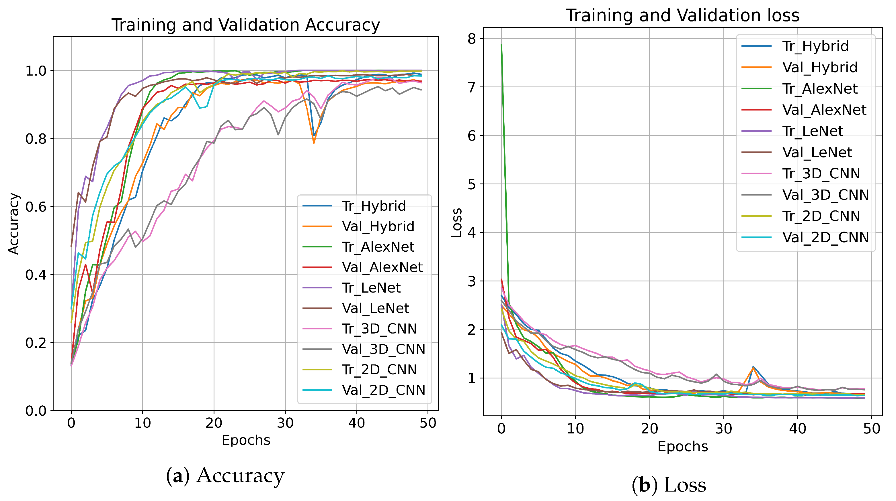
where and are true and false positive, and are true and false negative, respectively. For fair comparison purposes, the learning rate for all these models including hybrid models is set to 0.001, Relu as the activation function for all layers except the output layer on which Softmax is used, patch size is a set of 15, and, for all the experiments, the 15 most informative bands have been selected using principal component analysis to reduce the computational load. The convergence, accuracy, and loss of our proposed regularization technique with several CNN models for 50 epochs are presented in Figure 1. From loss and accuracy curves, one can conclude that the regularization has faster convergence.
3.1. Indian Pines
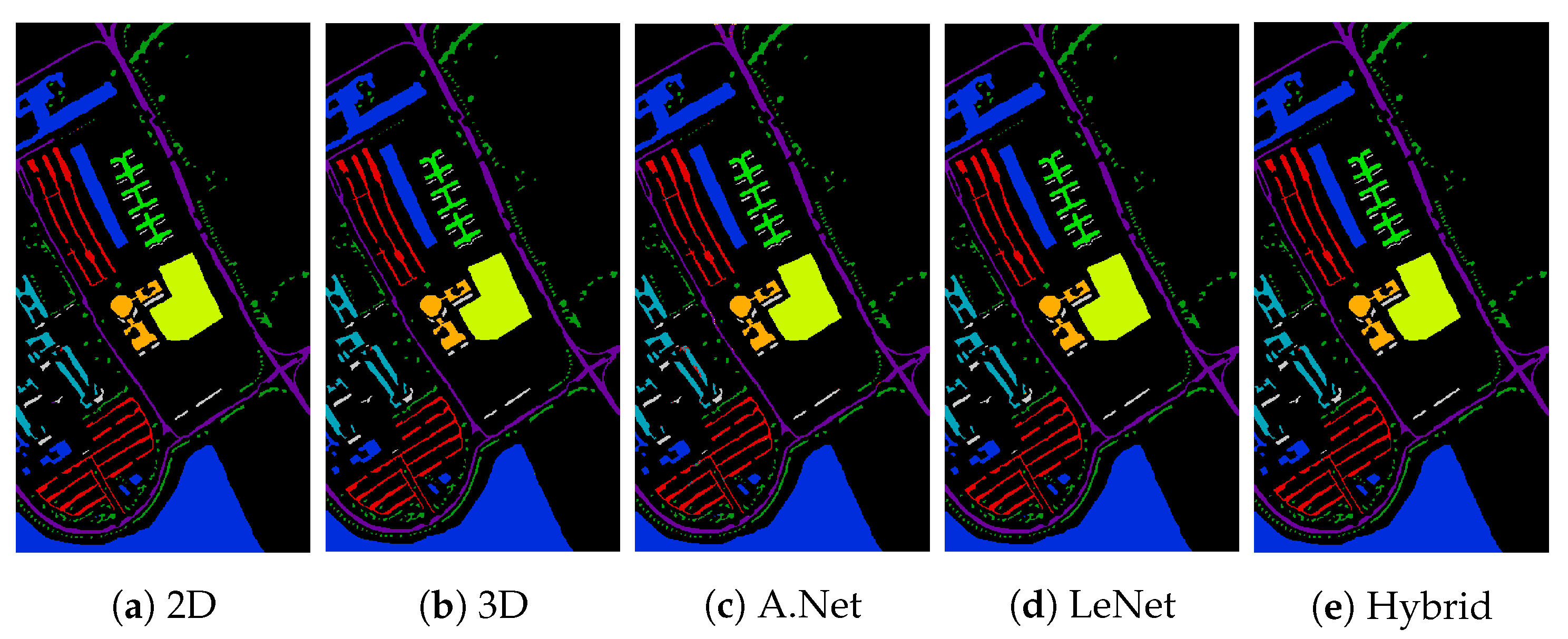
The Indian Pines (IP) dataset is acquired using an AVIRIS sensor over the northwestern Indiana test site. IP data consist of spatial dimensions and 224 spectral dimensions with a total of 16 classes in which all are not mutually exclusive. Some of the water absorption bands are removed, and the remaining 200 bands are used for the experimental process. These data consist of 2/3 agriculture, 1/3 forest, and other vegetation. Less than 5% of total coverage consists of crops that are in an early stage of growth. Building, low-density housing, two dual-lane highways, small roads, and a railway line are also a part of it. Further details about the experimental datasets can be found at [48]. Table 1 and Figure 2 present an in-depth comparative accuracy analysis on the IP dataset.
3.2. Pavia University
The Pavia University (PU) dataset acquired using a Reflective Optics System Imaging Spectrometer (ROSIS) optical sensor over Pavia in northern Italy. The PU dataset is distinguished into nine different classes. PU consists of spatial samples per spectral band and 103 spectral bands with a spatial resolution of 1.3 m. Further details about the experimental datasets can be found at [48]. Table 2 and Figure 3 present in-depth comparative accuracy analysis on the PU dataset.
3.3. Salinas
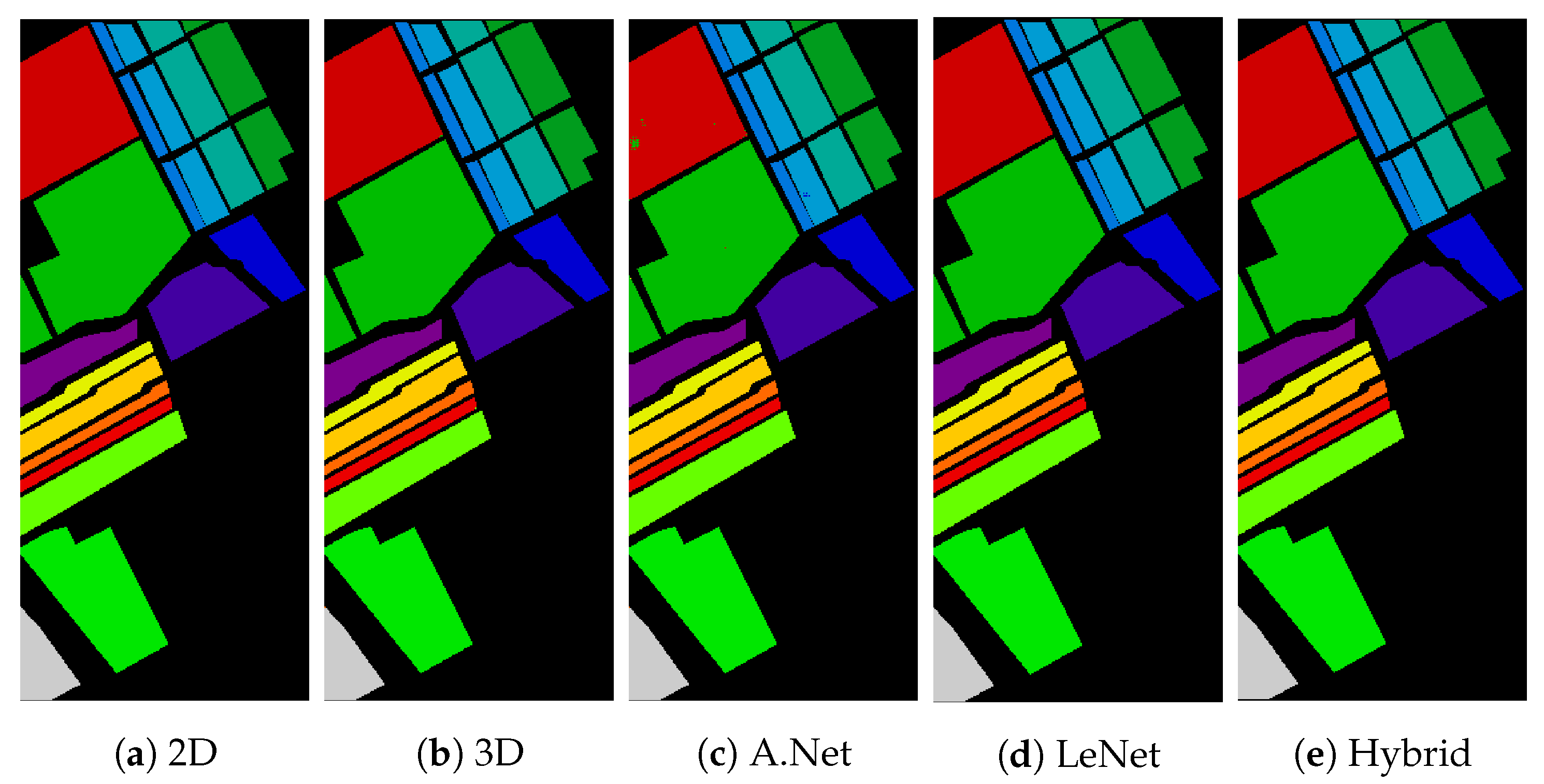
The Salinas (SA) dataset was acquired using an AVIRIS sensor over Salinas Valley, California and consists of 16 different classes—for instance, vineyard fields, vegetables, and bare soils. SA consists of 224 spectral bands in which each band is of size with a m spatial resolution. A few water absorption bands 108–112, 154–167, and 224 are removed before analysis. Further details about the experimental datasets can be found at [48]. Table 3 and Figure 4 present an in-depth comparative accuracy analysis on the Salinas dataset.
4. Comparison with State-of-the-Art Models
In all experimental results, the training, validation, and test sets are selected using a 5-fold cross-validation process with 25, 25, and 50% samples for training, validation, and test sets, respectively. The hybrid and all other competing models are trained using a patch size because the classification performance strongly depends on the patch size, in which, if the patch size is too big, then the model may take pixels from various classes, whereas, if the patch size is too small, the model may decrease the inter-class diversity in samples. Hence, in both cases, the ultimate result will be in terms of a higher misclassification rate, leading to low generalization performance. Therefore, an appropriate patch size needs to be selected before the final experimental setup. The patch size selected in these experiments is based on the hit and trial method (i.e., provided the best accuracy).
The experimental results on benchmark HSI datasets are presented in Table 4. From these results, one can conclude that the proposed regularization process significantly improves the performance, in terms of accuracy, speed of convergence, and computational time. For comparison purposes, the framework, i.e., regularization for the Hybrid CNN model, is compared with various state-of-the-art works published in recent years. From the experimental results presented in Table 4, one can conclude that regularization with Hybrid CNN has obtained better results as compared to the state-of-the-art frameworks and, to some extent, outperformed with respect to the other models. The comparative models include a Support Vector Machine (SVM) with and without any grid optimization, Multi-layer Perceptron (MLP) having four fully connected layers with dropout, a 2D CNN model proposed by Sharma et al. [21], a semi-supervised CNN model proposed by Liu et al. [22], a 3D CNN model proposed by Hamida et al. [23], a hybrid CNN model proposed by Lee et al. [24] that consists of two 3D and eight 2D convolutional layers, a simple and compact 3D CNN model proposed by Chen et al. [25] that consists of three 3D convolutional layers, and a lightweight 3D CNN model proposed by Li et al. [26] that consists of two 3D convolutional layers and a fully connected layer. Li’s work is different from traditional 3D CNN models as it uses fixed spatial-sized 3D convolutional layers with slight changes in spectral depth. Finally, multi-scale-3D-CNN [27], a fast and compact 3D-CNN (FC-3D-CNN) [20], and three different versions of Hybrid Depth-Separable Residual Network [28] were included.
All of the comparative models are being trained as per the settings mentioned in their respective papers except for the number of dimensions and patch size (i.e., 15 dimensions selected using PCA, and path size). The experimental results listed in Table 4 show that the proposed framework has significantly improved results as compared to the other methods with fewer training samples.
5. Conclusions
The paper proposed a regularized CNN feature hierarchy for HSIC, in which the loss contribution is considered as a mixture of entropy between a predicted distribution and the one-hot-encoding, and the entropy between the predicted and noise distribution. Several other regularization techniques (e.g., dropout, L1, L2, etc.) have also been used; however, these techniques, to some extent, lead to predicting the samples extremely confidently, which is not good from a generalization point of view. Therefore, this work proposed the use of an entropy-based regularization process to improve the generalization performance using soft labels. These soft labels are the weighted average of the hard labels and uniform distribution over entire ground truths. The entropy-based regularization process prevents CNN from becoming over-confident, while learning and predicting thus improves the model calibration and beam-search. Extensive experiments have confirmed that the proposed pipeline outperformed several state-of-the-art methods.
Author Contributions
Conceptualization, M.A.; Formal analysis, M.A. and S.D.; Funding acquisition, M.M.; Investigation, M.A. and S.D.; Methodology, M.A.; Project administration, M.M.; Supervision, M.M. and S.D.; Validation, M.A. and S.D.; Visualization, M.A. and M.M.; Writing—original draft, M.A., M.M., and S.D.; Writing—review and editing, M.A., M.M., and S.D. All authors have read and agreed to the published version of the manuscript.
Funding
This research received no external funding.
Institutional Review Board Statement
Not applicable.
Informed Consent Statement
Not applicable.
Data Availability Statement
Not applicable.
Conflicts of Interest
The authors declare no conflict of interest.
References
- Alcolea, A.; Paoletti, M.E.; Haut, J.M.; Resano, J.; Plaza, A. Inference in Supervised Spectral Classifiers for On-Board Hyperspectral Imaging: An Overview. Remote Sens. 2020, 12, 534. [Google Scholar] [CrossRef] [Green Version]
- Khabbazan, S.; Vermunt, P.; Steele-Dunne, S.; Ratering Arntz, L.; Marinetti, C.; van der Valk, D.; Iannini, L.; Molijn, R.; Westerdijk, K.; van der Sande, C. Crop Monitoring Using Sentinel-1 Data: A Case Study from The Netherlands. Remote Sens. 2019, 11, 1887. [Google Scholar] [CrossRef] [Green Version]
- Oddi, L.; Cremonese, E.; Ascari, L.; Filippa, G.; Galvagno, M.; Serafino, D.; Cella, U.M.d. Using UAV Imagery to Detect and Map Woody Species Encroachment in a Subalpine Grassland: Advantages and Limits. Remote Sens. 2021, 13, 1239. [Google Scholar] [CrossRef]
- Sun, X.; Wu, W.; Li, X.; Xu, X.; Li, J. Vegetation Abundance and Health Mapping Over Southwestern Antarctica Based on WorldView-2 Data and a Modified Spectral Mixture Analysis. Remote Sens. 2021, 13, 166. [Google Scholar] [CrossRef]
- Moniruzzaman, M.; Thakur, P.K.; Kumar, P.; Ashraful Alam, M.; Garg, V.; Rousta, I.; Olafsson, H. Decadal Urban Land Use/Land Cover Changes and Its Impact on Surface Runoff Potential for the Dhaka City and Surroundings Using Remote Sensing. Remote Sens. 2021, 13, 83. [Google Scholar] [CrossRef]
- Wang, B.; Shao, Q.; Song, D.; Li, Z.; Tang, Y.; Yang, C.; Wang, M. A Spectral-Spatial Features Integrated Network for Hyperspectral Detection of Marine Oil Spill. Remote Sens. 2021, 13, 1568. [Google Scholar] [CrossRef]
- Menon, N.; George, G.; Ranith, R.; Sajin, V.; Murali, S.; Abdulaziz, A.; Brewin, R.J.W.; Sathyendranath, S. Citizen Science Tools Reveal Changes in Estuarine Water Quality Following Demolition of Buildings. Remote Sens. 2021, 13, 1683. [Google Scholar] [CrossRef]
- Ayaz, H.; Ahmad, M.; Sohaib, A.; Yasir, M.N.; Zaidan, M.A.; Ali, M.; Khan, M.H.; Saleem, Z. Myoglobin-Based Classification of Minced Meat Using Hyperspectral Imaging. Appl. Sci. 2020, 10, 6862. [Google Scholar] [CrossRef]
- Ayaz, H.; Ahmad, M.; Mazzara, M.; Sohaib, A. Hyperspectral Imaging for Minced Meat Classification Using Nonlinear Deep Features. Appl. Sci. 2020, 10, 7783. [Google Scholar] [CrossRef]
- Khan, M.H.; Zainab, S.; Ahmad, M.; Sohaib, A.; Ayaz, H.; Mazzara, M. Hyperspectral Imaging for Color Adulteration Detection in Red Chili. Appl. Sci. 2020, 10, 5955. [Google Scholar] [CrossRef]
- Khan, M.H.; Saleem, Z.; Ahmad, M.; Sohaib, A.; Ayaz, H.; Mazzara, M.; Raza, R.A. Hyperspectral imaging-based unsupervised adulterated red chili content transformation for classification: Identification of red chili adulterants. Neural Comput. Appl. 2021. [Google Scholar] [CrossRef]
- Saleem, Z.; Khan, M.H.; Ahmad, M.; Sohaib, A.; Ayaz, H.; Mazzara, M. Prediction of Microbial Spoilage and Shelf-Life of Bakery Products Through Hyperspectral Imaging. IEEE Access 2020, 8, 176986–176996. [Google Scholar] [CrossRef]
- Ahmad, M.; Shabbir, S.; Raza, R.A.; Mazzara, M.; Distefano, S.; Khan, A.M. Hyperspectral Image Classification: Artifacts of Dimension Reduction on Hybrid CNN. arXiv 2021, arXiv:2101.10532. [Google Scholar]
- Wang, J.; Huang, R.; Guo, S.; Li, L.; Zhu, M.; Yang, S.; Jiao, L. NAS-Guided Lightweight Multiscale Attention Fusion Network for Hyperspectral Image Classification. IEEE Trans. Geosci. Remote Sens. 2021, 1–14. [Google Scholar] [CrossRef]
- Shabbir, S.; Ahmad, M. Hyperspectral Image Classification–Traditional to Deep Models: A Survey for Future Prospects. arXiv 2021, arXiv:2101.06116. [Google Scholar]
- Ahmad, M.; Khan, A.M.; Hussain, R.; Protasov, S.; Chow, F.; Khattak, A.M. Unsupervised geometrical feature learning from hyperspectral data. In Proceedings of the IEEE Symposium Series on Computational Intelligence (SSCI), Athens, Greece, 6–9 December 2016; IEEE Computational Intelligence Socity: New York, NY, USA, 2016; pp. 1–6. [Google Scholar]
- Ahmad, M. Ground Truth Labeling and Samples Selection for Hyperspectral Image Classification. Optik 2021, 230, 166267. [Google Scholar] [CrossRef]
- Ahmad, M.; Shabbir, S.; Oliva, D.; Mazzara, M.; Distefano, S. Spatial-prior generalized fuzziness extreme learning machine autoencoder-based active learning for hyperspectral image classification. Optik 2020, 206, 163712. [Google Scholar] [CrossRef]
- Jia, S.; Jiang, S.; Lin, Z.; Li, N.; Xu, M.; Yu, S. A survey: Deep learning for hyperspectral image classification with few labeled samples. Neurocomputing 2021, 448, 179–204. [Google Scholar] [CrossRef]
- Ahmad, M.; Khan, A.M.; Mazzara, M.; Distefano, S.; Ali, M.; Sarfraz, M.S. A Fast and Compact 3D CNN for Hyperspectral Image Classification. In IEEE Geosci. Remote Sens. Lett. 2020, 1–5. [Google Scholar] [CrossRef]
- Xie, Z.; Li, Y.; Niu, J.; Shi, L.; Wang, Z.; Lu, G. Hyperspectral face recognition based on sparse spectral attention deep neural networks. Opt. Express 2020, 28, 36286–36303. [Google Scholar] [CrossRef]
- Liu, B.; Yu, X.; Zhang, P.; Tan, X.; Yu, A.; Xue, Z. A semi-supervised convolutional neural network for hyperspectral image classification. Remote Sens. Lett. 2017, 8, 839–848. [Google Scholar] [CrossRef]
- Ben Hamida, A.; Benoit, A.; Lambert, P.; Ben Amar, C. 3D Deep Learning Approach for Remote Sensing Image Classification. IEEE Trans. Geosci. Remote Sens. 2018, 56, 4420–4434. [Google Scholar] [CrossRef] [Green Version]
- Lee, H.; Kwon, H. Contextual deep CNN based hyperspectral classification. In Proceedings of the 2016 IEEE International Geoscience and Remote Sensing Symposium (IGARSS), Beijing, China, 10–15 July 2016; pp. 3322–3325. [Google Scholar] [CrossRef]
- Chen, Y.; Jiang, H.; Li, C.; Jia, X.; Ghamisi, P. Deep Feature Extraction and Classification of Hyperspectral Images Based on Convolutional Neural Networks. IEEE Trans. Geosci. Remote Sens. 2016, 54, 6232–6251. [Google Scholar] [CrossRef] [Green Version]
- Li, Y.; Zhang, H.; Shen, Q. Spectral–Spatial Classification of Hyperspectral Imagery with 3D Convolutional Neural Network. Remote Sens. 2017, 9, 67. [Google Scholar] [CrossRef] [Green Version]
- He, M.; Li, B.; Chen, H. Multi-scale 3D deep convolutional neural network for hyperspectral image classification. In Proceedings of the 2017 IEEE International Conference on Image Processing (ICIP), Beijing, China, 17–20 September 2017; pp. 3904–3908. [Google Scholar]
- Zhao, C.; Zhao, H.; Wang, G.; Chen, H. Hybrid Depth-Separable Residual Networks for Hyperspectral Image Classification. Complexity 2020, 2020, 4608647. [Google Scholar] [CrossRef]
- Yang, X.; Zhang, X.; Ye, Y.; Lau, R.; Lu, S.; Li, X.; Huang, X. Synergistic 2D/3D Convolutional Neural Network for Hyperspectral Image Classification. Remote Sens. 2020, 12, 2033. [Google Scholar] [CrossRef]
- Rumelhart, D.E.; Hinton, G.E.; Williams, R.J. Learning Representations by Back-Propagating Errors. In Neurocomputing: Foundations of Research; MIT Press: Cambridge, MA, USA, 1988; pp. 696–699. [Google Scholar]
- Sha, H.; Al Hasan, M.; Mohler, G. Learning Network Event Sequences Using Long Short-Term Memory and Second-Order Statistic Loss. Stat. Anal. Data Min. 2021, 14, 61–73. [Google Scholar] [CrossRef]
- Li, H.C.; Li, S.S.; Hu, W.S.; Feng, J.H.; Sun, W.W.; Du, Q. Recurrent Feedback Convolutional Neural Network for Hyperspectral Image Classification. IEEE Geosci. Remote Sens. Lett. 2021, 1–5. [Google Scholar] [CrossRef]
- Lei, R.; Zhang, C.; Du, S.; Wang, C.; Zhang, X.; Zheng, H.; Huang, J.; Yu, M. A non-local capsule neural network for hyperspectral remote sensing image classification. Remote Sens. Lett. 2021, 12, 40–49. [Google Scholar] [CrossRef]
- Bi, H.; Santos-Rodriguez, R.; Flach, P. Polsar Image Classification via Robust Low-Rank Feature Extraction and Markov Random Field. In Proceedings of the IGARSS 2020—2020 IEEE International Geoscience and Remote Sensing Symposium, Waikoloa, HI, USA, 26 September–2 October 2020; pp. 708–711. [Google Scholar] [CrossRef]
- Szegedy, C.; Vanhoucke, V.; Ioffe, S.; Shlens, J.; Wojna, Z. Rethinking the Inception Architecture for Computer Vision. In Proceedings of the 2016 IEEE Conference on Computer Vision and Pattern Recognition (CVPR), Las Vegas, NV, USA, 27–30 June 2016. [Google Scholar] [CrossRef] [Green Version]
- Zhang, C.; Han, M. Multi-feature hyperspectral image classification with L2,1 norm constrained joint sparse representation. Int. J. Remote Sens. 2021, 42, 4789–4808. [Google Scholar] [CrossRef]
- Real, E.; Aggarwal, A.; Huang, Y.; Le, Q.V. Regularized Evolution for Image Classifier Architecture Search. Proc. AAAI Conf. Artif. Intell. 2019, 33, 4780–4789. [Google Scholar] [CrossRef] [Green Version]
- Zoph, B.; Vasudevan, V.; Shlens, J.; Le, Q.V. Learning Transferable Architectures for Scalable Image Recognition. CoRR 2017, arXiv:1707.07012. [Google Scholar]
- Yin, B.; Cui, B. Multi-feature extraction method based on Gaussian pyramid and weighted voting for hyperspectral image classification. In Proceedings of the 2021 IEEE International Conference on Consumer Electronics and Computer Engineering (ICCECE), Guangzhou, China, 15–17 January 2021; pp. 645–648. [Google Scholar] [CrossRef]
- Zhou, H.; Song, L.; Chen, J.; Zhou, Y.; Wang, G.; Yuan, J.; Zhang, Q. Rethinking Soft Labels for Knowledge Distillation: A Bias-Variance Tradeoff Perspective. arXiv 2021, arXiv:cs.LG/2102.00650. [Google Scholar]
- Pham, H.H.; Le, T.T.; Tran, D.Q.; Ngo, D.T.; Nguyen, H.Q. Interpreting chest X-rays via CNNs that exploit hierarchical disease dependencies and uncertainty labels. Neurocomputing 2021, 437, 186–194. [Google Scholar] [CrossRef]
- Song, M.; Zhao, Y.; Wang, S.; Han, M. Word Similarity Based Label Smoothing in Rnnlm Training for ASR. In Proceedings of the 2021 IEEE Spoken Language Technology Workshop (SLT), Shenzhen, China, 19–22 January 2021; pp. 280–285. [Google Scholar] [CrossRef]
- Xie, F.; Gao, Q.; Jin, C.; Zhao, F. Hyperspectral Image Classification Based on Superpixel Pooling Convolutional Neural Network with Transfer Learning. Remote Sens. 2021, 13, 930. [Google Scholar] [CrossRef]
- Yang, X.; Song, Z.; King, I.; Xu, Z. A Survey on Deep Semi-supervised Learning. arXiv 2021, arXiv:cs.LG/2103.00550. [Google Scholar]
- Carneiro, T.; Da Nóbrega, R.V.M.; Nepomuceno, T.; Bian, G.B.; De Albuquerque, V.H.C.; Reboucas Filho, P.P. Performance Analysis of Google Colaboratory as a Tool for Accelerating Deep Learning Applications. IEEE Access 2018, 6, 61677–61685. [Google Scholar] [CrossRef]
- Mei, S.; Chen, X.; Zhang, Y.; Li, J.; Plaza, A. Accelerating Convolutional Neural Network-Based Hyperspectral Image Classification by Step Activation Quantization. IEEE Trans. Geosci. Remote Sens. 2021, 1–12. [Google Scholar] [CrossRef]
- Yuan, Y.; Wang, C.; Jiang, Z. Proxy-Based Deep Learning Framework for Spectral-Spatial Hyperspectral Image Classification: Efficient and Robust. IEEE Trans. Geosci. Remote Sens. 2021, 1–15. [Google Scholar] [CrossRef]
- Hyperspectral Datasets Description. 2021. Available online: http://www.ehu.eus/ccwintco/index.php/Hyperspectral_Remote_Sensing_Scenes (accessed on 1 April 2020).
Figure 1.
Accuracy and loss for training and validation sets on Indian Pines for 50 epochs.

Figure 2.
Indian Pines: Classification accuracy: (a) 2D-CNN = 98.94%; (b) 3D CNN = 91.57%; (c) AlexNet = 97.65%; (d) LeNet = 98.14%; and (e) Hybrid = 99.29%.
Figure 2.
Indian Pines: Classification accuracy: (a) 2D-CNN = 98.94%; (b) 3D CNN = 91.57%; (c) AlexNet = 97.65%; (d) LeNet = 98.14%; and (e) Hybrid = 99.29%.

Figure 3.
Pavia University: Classification accuracy: (a) 2D-CNN = 99.9070%; (b) 3D CNN = 99.9256%; (c) AlexNet = 99.0768%; (d) LeNet = 99.9318%; and (e) Hybrid = 99.9628%.
Figure 3.
Pavia University: Classification accuracy: (a) 2D-CNN = 99.9070%; (b) 3D CNN = 99.9256%; (c) AlexNet = 99.0768%; (d) LeNet = 99.9318%; and (e) Hybrid = 99.9628%.

Figure 4.
Salinas: Classification accuracy: (a) 2D-CNN = 99.9876%; (b) 3D CNN = 99.9794%; (c) AlexNet = 99.8559%; (d) LeNet = 100.0%; and (e) Hybrid = 100.0%.
Figure 4.
Salinas: Classification accuracy: (a) 2D-CNN = 99.9876%; (b) 3D CNN = 99.9794%; (c) AlexNet = 99.8559%; (d) LeNet = 100.0%; and (e) Hybrid = 100.0%.


Table 1.
Indian Pines: Performance analysis of different state-of-the-art models trained using regularization technique.
Table 1.
Indian Pines: Performance analysis of different state-of-the-art models trained using regularization technique.
| Class | Train/Val/Test | 2D | 3D | AlexNet | LeNet | Hybrid |
|---|---|---|---|---|---|---|
| Alfalfa | 11/12/23 | 100 | 91.3043 | 95.6521 | 82.6086 | 100 |
| Corn-notill | 357/357/714 | 98.3193 | 93.5574 | 97.3389 | 97.0588 | 98.8795 |
| Corn-mintill | 207/208/415 | 99.5180 | 66.7469 | 98.3132 | 99.5180 | 99.5180 |
| Corn | 59/59/118 | 94.0677 | 90.6779 | 93.2203 | 99.1525 | 100 |
| Grass–pasture | 121/121/242 | 98.3471 | 97.1074 | 96.2809 | 94.2148 | 96.2809 |
| Grass–trees | 182/183/365 | 98.9041 | 97.5342 | 98.3561 | 98.9041 | 99.7260 |
| Grass-mowed | 7/7/14 | 92.8571 | 92.8571 | 100 | 100 | 100 |
| Hay-windrowed | 119/120/239 | 100 | 100 | 100 | 100 | 100 |
| Oats | 5/5/10 | 70 | 0 | 100 | 70 | 100 |
| Soybean-notill | 243/243/486 | 98.5596 | 82.3045 | 93.6213 | 99.3827 | 97.9423 |
| Soybean-mintill | 614/614/1228 | 99.6742 | 92.4267 | 97.8013 | 99.9185 | 99.8371 |
| Soybean-clean | 148/149/297 | 97.6430 | 98.6531 | 96.9696 | 95.2861 | 99.6632 |
| Wheat | 51/51/102 | 99.0196 | 98.0392 | 100 | 99.0196 | 99.0196 |
| Woods | 316/317/633 | 99.8420 | 99.3680 | 99.5260 | 98.8941 | 99.8420 |
| Buildings | 96/97/193 | 99.4818 | 90.6735 | 100 | 91.1917 | 99.4818 |
| Stone–steel | 23/23/46 | 100 | 97.8260 | 100 | 93.4782 | 100 |
| Training Time | 55.6695 | 250.1662 | 919.5566 | 61.8763 | 248.5993 | |
| Test Time | 1.4897 | 4.0402 | 5.6891 | 1.2752 | 3.9997 | |
| Overall Accuracy | 98.9463 | 91.5707 | 97.6585 | 98.14634 | 99.2975 | |
| Average Accuracy | 98.7980 | 86.8173 | 97.9425 | 94.9142 | 99.3869 | |
| Kappa () | 96.6396 | 90.3561 | 97.3312 | 97.8853 | 99.1990 | |
Table 2.
Pavia University: Performance analysis of different state-of-the-art models trained using regularization technique.
Table 2.
Pavia University: Performance analysis of different state-of-the-art models trained using regularization technique.
| Class | Train/Val/Test | 2D | 3D | AlexNet | LeNet | Hybrid |
|---|---|---|---|---|---|---|
| Asphalt | 1658/1658/3316 | 100 | 100 | 98.9143 | 100 | 100 |
| Meadows | 4662/4662/9324 | 100 | 99.9892 | 100 | 100 | 100 |
| Gravel | 524/525/1049 | 99.5233 | 99.3326 | 95.5195 | 99.4280 | 99.6186 |
| Trees | 766/766/1532 | 99.6736 | 100 | 98.8250 | 99.7389 | 100 |
| Painted | 336/337/673 | 100 | 100 | 100 | 100 | 100 |
| Soil | 1257/1257/2514 | 100 | 100 | 99.9602 | 100 | 100 |
| Bitumen | 332/333/665 | 100 | 100 | 99.6992 | 100 | 100 |
| Bricks | 920/921/1841 | 99.8913 | 99.8913 | 97.9359 | 100 | 99.8913 |
| Shadows | 237/237/74 | 99.3670 | 99.5780 | 98.5232 | 99.7890 | 100 |
| Training Time | 296.0174 | 1145.9233 | 4716.4900 | 308.6389 | 1143.4996 | |
| Test Time | 5.7400 | 14.8634 | 24.1701 | 4.5054 | 15.5904 | |
| Overall Accuracy | 99.9298 | 99.9438 | 99.3033 | 99.9485 | 99.9719 | |
| Average Accuracy | 99.8283 | 99.8657 | 98.8197 | 99.8839 | 99.9455 | |
| Kappa () | 99.9070 | 99.9256 | 99.0768 | 99.9318 | 99.9628 | |
Table 3.
Salinas: Performance analysis of different state-of-the-art models trained using regularization technique.
Table 3.
Salinas: Performance analysis of different state-of-the-art models trained using regularization technique.
| Class | Train/Val/Test | 2D | 3D | AlexNet | LeNet | Hybrid |
|---|---|---|---|---|---|---|
| Weeds 1 | 502/502/1005 | 100 | 100 | 100 | 100 | 100 |
| Weeds 2 | 931/931/1863 | 100 | 100 | 100 | 100 | 100 |
| Fallow | 494/494/988 | 100 | 100 | 100 | 100 | 100 |
| Fallow rough plow | 348/348/698 | 100 | 100 | 100 | 100 | 100 |
| Fallow smooth | 669/669/1340 | 100 | 100 | 99.7012 | 100 | 100 |
| Stubble | 990/990/1980 | 100 | 100 | 100 | 100 | 100 |
| Celery | 894/894/1790 | 99.9441 | 100 | 100 | 100 | 100 |
| Grapes untrained | 2817/2818/5636 | 99.9822 | 100 | 99.9822 | 100 | 100 |
| Soil vinyard develop | 1550/1551/3102 | 100 | 100 | 100 | 100 | 100 |
| Corn Weeds | 819/820/1639 | 100 | 100 | 100 | 100 | 100 |
| Lettuce 4wk | 267/267/534 | 100 | 100 | 100 | 100 | 100 |
| Lettuce 5wk | 481/482/963 | 100 | 100 | 100 | 100 | 100 |
| Lettuce 6wk | 229/229/458 | 100 | 100 | 100 | 100 | 100 |
| Lettuce 7wk | 267/268/535 | 100 | 99.6261 | 100 | 100 | 100 |
| Vinyard untrained | 1817/1817/3634 | 99.8130 | 99.9174 | 99.1744 | 100 | 100 |
| Vinyard trellis | 451/452/904 | 100 | 100 | 100 | 100 | 100 |
| Training Time | — | 257.9992 | 1256.1199 | 4667.9047 | 288.3353 | 1267.9766 |
| Test Time | — | 7.3995 | 16.8058 | 27.8388 | 6.3860 | 19.2670 |
| Overall Accuracy | — | 99.9889 | 99.9815 | 99.8706 | 100.0 | 100.0 |
| Average Accuracy | — | 99.9837 | 99.9714 | 99.9286 | 100.0 | 100.0 |
| Kappa () | — | 99.9876 | 99.9794 | 99.8559 | 100.0 | 100.0 |
Table 4.
Experimental comparison with state-of-the-art models.
| Methods | Salinas Full Scene | Indian Pines | ||||
|---|---|---|---|---|---|---|
| OA | AA | Kappa | OA | AA | Kappa | |
| MLP | 79.79 | 67.37 | 77.40 | 87.57 | 89.07 | 85.80 |
| SVM-Grid | 67.39 | 45.89 | 62.80 | 87.93 | 88.02 | 86.20 |
| SVM | 92.95 | 94.60 | 92.11 | 85.30 | 79.03 | 83.10 |
| FC-3D-CNN [20] | 98.06 | 98.80 | 97.85 | 98.20 | 96.46 | 97.95 |
| Xie et al. [21] | 93.35 | 91.88 | 92.60 | 95.64 | 96.01 | 95.10 |
| Liu et al. [22] | 84.27 | 79.10 | 82.50 | 89.56 | 89.32 | 88.10 |
| 3D-CNN [23] | 85.00 | 89.63 | 83.20 | 82.62 | 76.51 | 79.25 |
| Lee et al. [24] | 84.14 | 73.27 | 82.30 | 87.87 | 83.42 | 86.10 |
| Chen et al. [25] | 86.83 | 92.08 | 85.50 | 93.20 | 95.51 | 92.30 |
| Li [26] | 88.62 | 86.84 | 87.40 | 94.22 | 96.71 | 93.40 |
| MS-3D-CNN [27] | 94.69 | 94.03 | 94.10 | 91.87 | 92.21 | 90.80 |
| Zhao et al. [28] | 98.89 | 98.88 | 98.85 | 95.86 | 96.08 | 95.09 |
| SyCNN-S [29] | 97.44 | 98.46 | 97.20 | 95.90 | 97.84 | 95.30 |
| SyCNN-D [29] | 97.76 | 98.95 | 97.50 | 96.13 | 98.08 | 95.60 |
| SyCNN-ATT [29] | 98.92 | 99.35 | 98.80 | 97.31 | 98.43 | 96.90 |
| Regularized AlexNet | 99.87 | 99.92 | 99.85 | 97.65 | 97.94 | 97.33 |
| Regularized LeNet | 100.0 | 100.0 | 100.0 | 98.14 | 94.91 | 97.88 |
| Regularized 2D | 99.98 | 99.98 | 99.98 | 98.94 | 98.79 | 96.63 |
| Regularized 3D | 99.98 | 99.97 | 99.97 | 91.57 | 86.81 | 90.35 |
| Regularized Hybrid | 100.0 | 100.0 | 100.0 | 99.29 | 99.38 | 99.19 |
Publisher’s Note: MDPI stays neutral with regard to jurisdictional claims in published maps and institutional affiliations. |
© 2021 by the authors. Licensee MDPI, Basel, Switzerland. This article is an open access article distributed under the terms and conditions of the Creative Commons Attribution (CC BY) license (https://creativecommons.org/licenses/by/4.0/).
Share and Cite
MDPI and ACS Style
Ahmad, M.; Mazzara, M.; Distefano, S. Regularized CNN Feature Hierarchy for Hyperspectral Image Classification. Remote Sens. 2021, 13, 2275. https://doi.org/10.3390/rs13122275
AMA Style
Ahmad M, Mazzara M, Distefano S. Regularized CNN Feature Hierarchy for Hyperspectral Image Classification. Remote Sensing. 2021; 13(12):2275. https://doi.org/10.3390/rs13122275
Chicago/Turabian StyleAhmad, Muhammad, Manuel Mazzara, and Salvatore Distefano. 2021. "Regularized CNN Feature Hierarchy for Hyperspectral Image Classification" Remote Sensing 13, no. 12: 2275. https://doi.org/10.3390/rs13122275
Note that from the first issue of 2016, this journal uses article numbers instead of page numbers. See further details here.