Performance Comparison of Oil Spill and Ship Classification from X-Band Dual- and Single-Polarized SAR Image Using Support Vector Machine, Random Forest, and Deep Neural Network

Abstract

It is well known that the polarization characteristics in X-band synthetic aperture radar (SAR) image analysis can provide us with additional information for marine target classification and detection. Normally, dual-and single-polarized SAR images are acquired by SAR satellites, and then we must determine how accurate the marine mapping performance from dual-polarized (pol) images is versus the marine mapping performance from the single-pol images in a given machine learning model. The purpose of this study is to compare the performance of single- and dual-pol SAR image classification achieved by the support vector machine (SVM), random forest (RF), and deep neural network (DNN) models. The test image is a TerraSAR-X dual-pol image acquired from the 2007 Kerch Strait oil spill event. For this, 824,026 pixels and 1,648,051 pixels were extracted from the image for the training and test, respectively, and sea, ship, oil, and land objects were classified from the image by using the three machine learning methods. The mean f1-scores of the SVM, RF, and DNN models resulting from the single-pol image were approximately 0.822, 0.882, and 0.889, respectively, and those from the dual-pol image were about 0.852, 0.908, and 0.898, respectively. The performance improvement achieved by dual-pol was about 3.6%, 2.9%, and 1% in SVM, RF, and DNN, respectively. The DNN model had the best performance (0.889) in the single-pol test while the RF model was best (0.908) in the dual-pol test. The performance improvement was approximately 2.1% and not noticeable. If the condition that dual-pol images have two-times lower spatial resolution versus single-pol images in the azimuth direction is considered, a small improvement may not be valuable. Therefore, the results show that the performance improvement by X-band dual-pol image may be not remarkable when classifying the sea, ships, oil spills, and sea and land surfaces.

1. Introduction

Synthetic aperture radar (SAR) has distinctive advantages in classifying marine features, such as ships and oil spills [1,2,3]. An SAR image is acquired by an active sensor that utilizes a longer wavelength electromagnetic wave than optical and thermal bands. The SAR characteristics enable us to provide almost constant quality data regardless of the weather or solar elevation [4]. Moreover, the radar backscattering signals from the sea, oil spills, and ships are different. The radar signal backscattered from the oil spill is reduced due to the dampened sea surface roughness [1,5,6] while the radar signal from ships is bounced more than twice between ships and the sea surface, which is called the corner effect. Thus, oil spills have a lower brightness value, while ships have a higher brightness value compared to the surrounding sea surface on the SAR images [7,8,9,10].

The polarimetric SAR (PolSAR) approach provides us with additional information of the marine target, and hence many studies have been performed on marine-target classification and detection using PolSAR images [3,11,12,13,14,15]. The polarization of a traditional SAR system is usually designed to transmit and receive two orthogonal polarizations of horizontal (H) or vertical (V) directions. Recently, compact polarization was introduced that exploits the degree between superpositioned horizontal and vertical polarization [14,15]. It has been known that the PolSAR approach is effective in reducing false alarm and omission errors because the backscattering characteristics of marine objects vary depending on the polarization [14,15]. To use the polarization property efficiently, the co-polarized phase difference (CPD) approach has been suggested for oil spill mapping, which exploits the inter-channel correlation of dual-polarized SAR data [12,15]. Brekke and Anfinsen (2010) have shown the potential of dual-polarized SAR data to detect ships in an ice-infested area with a suitable SAR statistical model [3] and Shirvany et al. (2012) have shown that the detection performance of ships depends on the combination of the polarized SAR data [14].

Machine learning approaches, including support vector machine (SVM), random forest (RF), artificial neural network (ANN), and convolutional neural network (CNN), have been recently applied to many research fields [16,17,18,19,20,21]. Since the approaches exploit the non-linear relationship between the various input data, they can remarkably improve the SAR-based detection performance of the marine targets of interest (TOI). The SAR-derived data, such as normalized intensity and texture maps, were employed as input data of machine learning approaches to reduce noise of the SAR image and enhance the contrast between the TOI and others [7,8,9,20,22,23]. Moreover, multi-polarized SAR-derived data have been applied to machine learning methods for obtaining additional information about TOI [1,21,24,25,26].

However, it is unclear how many machine learning models trained with dual-polarized SAR data improve pixel-wise target classification performance over single-polarized SAR data in marine TOI environments. Kim and Jung (2018) compared the oil spill mapping performance of single- and dual-polarized SAR data via ANN [17]. In the study, the probability peak on the lookalikes was reduced from 0.659 to 0.363 after adopting dual-polarized SAR data. The area under curves of receiver operating characteristics (ROC) curve for single- and dual-polarized input data were about 0.9503 and 0.9519, respectively. The difference was not noticeable in showing the performance improvement using dual-polarized SAR data [17]. Fan et al. 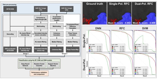(2019) introduced the U-Net architecture for ship detection using compact polarimetric SAR data and compared the performance achieved by single-, dual- and full-polarization [26]. The f1-scores among the different polarization modes were about 0.650, 0.863, and 0.912, respectively [26]. The research showed that the polarization data can improve the performance of ship detection. However, since the performance validation was tested by an object-wise approach, there was a limitation as well as performance improvements in distributed targets such as oil spills and land and sea surfaces, which have not been analyzed.

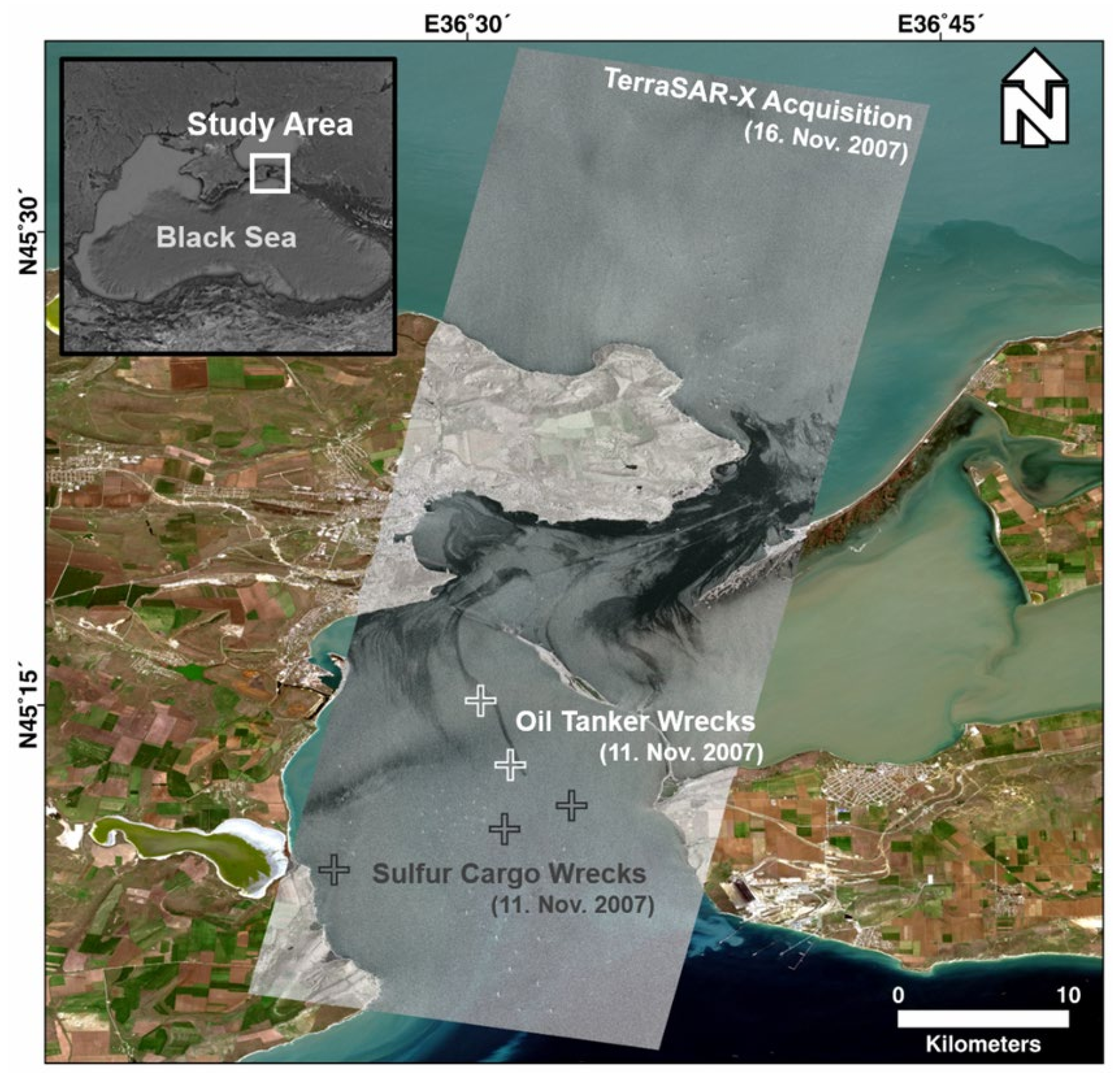
In this study, we compare the performance of SVM, RF, and deep neural network (DNN) approaches on marine target classification on ships, oil spills, and sea and land surfaces to analyze the effect of dual-polarized SAR data on pixel-wise target classification performance improvement of the machine learning models. For this, the TerraSAR-X image acquired from the oil spill accident in the Kerch Strait in November 2007 was used. The data was separated by two groups: (1) group 1 has three input data composed of VV-polarized normalized SAR intensity and texture maps and digital elevation model (DEM), and (2) group 2 has five input data consisting of Group 1′s input data and co-polarized coherence and CPD texture maps. Then, we trained the SVM, RF, and DNN models using the input data of Group 1 and 2, and evaluated the model performances, and finally, the classification performances achieved by three models and two input data groups were analyzed and compared.

2. Study Area and Data

On 11 November 2007, a heavy storm at 35 m/s and waves at 5 m/s broke a 3500 ton oil tanker into two pieces, which sank in the Kerch Strait [1,17,27,28]. In the aftermath of the accident, more than 1300 tons of oil were spilled, and most of the oil spread throughout the Kerch Strait along the current [1,27]. Several SAR data related to the oil spill accident were acquired from the COSMO-SkyMed, Radarsat-1, Envisat ASAR, and TerraSAR-X satellites. Among them, the TerraSAR-X stripmap image was acquired in dual polarization (pol) mode at 03:52, universal time (UT) on 16 November 2007. The dual-pol mode provides the orthogonal polarization of HH and VV. Furthermore, since the wind speed at the acquisition time was moderate (about 2 to 3 m/s), the oil spill area is well distinguished from the image. Figure 1 shows the study area, and the gray-scaled map shown in the middle of Figure 1 indicates the TerraSAR-X HH intensity image. Several features in the TerraSAR-X image are characterized by ships, oil spill areas, and land and sea surfaces.

In machine learning approaches, since the predictive model is trained based on the relationship between ground truth and input data, the wrong ground truth can lead to wrong classification results [7]. Conversely, the ability of classification is largely dependent on the quality of ground truth. Thus, the confident ground truth is required to validate and compare the classification performance of the SVM, RF, and DNN models. Ground truth data seen in Figure 2b was manually generated from TerraSAR-X intensity map by visual analysis. It is not difficult to define ships, and land and sea surfaces from the SAR intensity map. However, defining oil spills is not easy due to lookalikes. This is because pixel values of the lookalikes are darker than the surrounding ocean surface, such as oil spills [27]. As shown in the ground truth map, the pixels of oil spills, ships, and sea and land surfaces are composed of about 7.9%, 0.1%, 75.5%, and 16.6% in the test image, respectively. Figure 2c–f presents the ground truth maps magnified by the boxes A to D of Figure 2b. As shown in Figure 2c–f; (i) all the classes are present in Figure 2c; (ii) the sea, oil spill, and land classes are distributed with balance (Figure 2d); (iii) several ships can be found, and the lookalikes of oil spill areas are widely distributed in Figure 2e; and (iv) Figure 2f presents several ships and isolated oil spills.

3. Methodology

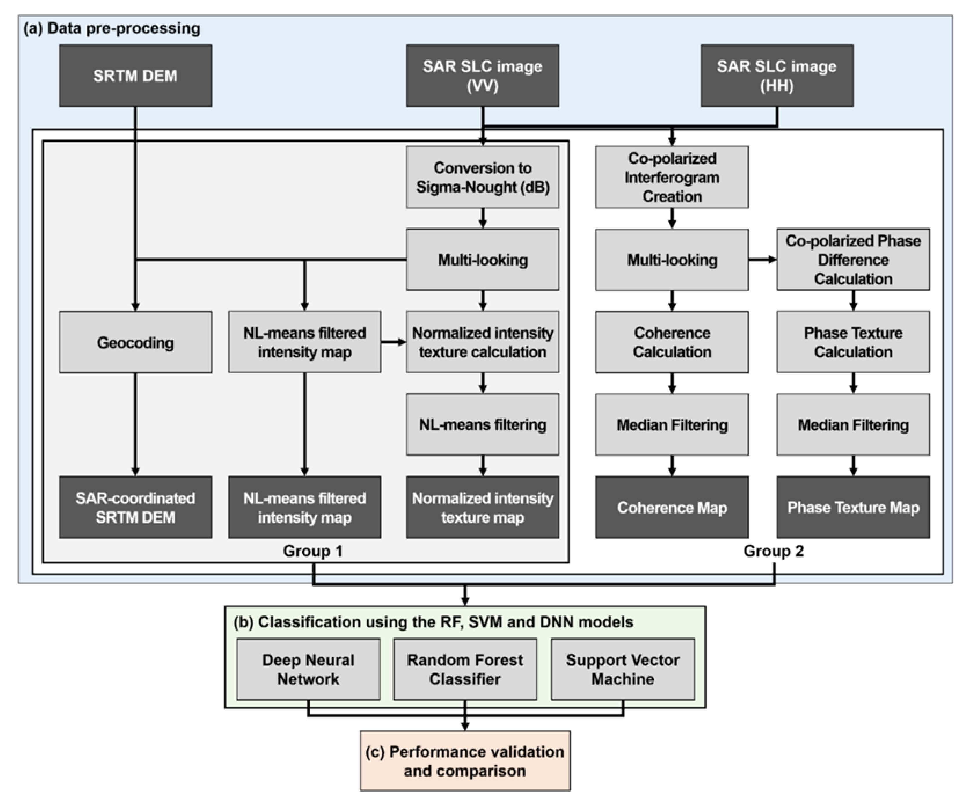
The detailed processing flow is seen in Figure 3. The data processing flow can be categorized into three main processing steps: (i) data pre-processing, (ii) classification using the RF, SVM, and DNN models, and (iii) performance validation and comparison.

First, the pre-processing step creates five normalized maps from the TerraSAR-X HH and VV single look complex (SLC) images and SRTM DEM to prepare the input data of the machine learning models. Among the five normalized maps, the SAR intensity map and SAR intensity texture map are created from the VV SLC image; the co-polarized coherence map and CPD texture map are generated from the phase difference between HH and VV SLC images, and the normalized topography map is produced from the SRTM DEM. To reduce the noise of the intensity map, multi-looking and a non-local mean filter with 5 × 5 kernel size are applied to the intensity map [29]. The normalized intensity texture map is generated by the root-mean-square of the difference between the NL-means filtered intensity map and multi-looked intensity map. The coherence map is created by the ensemble average of multi-looked co-polarized interferogram with a 5 × 5 moving window. The CPD map is calculated by estimating the standard deviation of the phase difference between the HH and VV SLC images with a 5 × 5 moving window. The geometry of SRTM DEM was converted to radar geometry by using look-up table, which calculated, by intensity, cross-correlation between the multi-looked intensity map and SRTM-simulated intensity map [17]. More details for the preprocessing can be found in [17]. Then, the created five maps were divided into two groups: (i) single-pol and (ii) dual-pol, to compare the classification performance between the two groups. The single-pol group consisted of the SAR intensity, SAR intensity texture, and topography maps, while the dual-pol group was composed of all five maps.

Second, the classification step is performed to classify ships, oil spills, and sea and land surfaces from the input data of the two groups using the SVM, RF, and DNN models. Normally, machine learning methods can be categorized as supervised learning, unsupervised learning, semi-supervised learning, and reinforcement learning [30]. The three models used in this study are of the supervised learning approaches. The different SVM, RF, and DNN models were selected to analyze and compare the classification performance between single-pol and dual-pol data. SVM is a representative machine learning model that can be used for the linear and non-linear classification or regression [30]. RF is an ensemble method of decision tree [30], and DNN is a deep multi-layer perception (MLP) neural network [19,30].

To train the models from the input data and estimate the classification performance, the training and test data were randomly extracted from the input data at a rate of 10% (824,025 pixels) and 20% (1,648,052 pixels), respectively. Training and test data do not overlap with each other. The pixel number of (training data and test data) for sea surface, oil spills, ship, and land classes were (618,149 and 1,236,251), (67,997 and 137,036), (474 and 917), and (137,405 and 273,848) pixels, respectively. The class majority was largely skewed on the sea and land pixels. The number of the training data in the ship class was minimal. Data imbalance can affect the final classification performance for each class [31]. In this study, the models were trained without consideration for the data imbalance problem. Thus, there is a limitation to comparing the performance of each class.

The hyperparameters of the SVM, RF, and DNN models were determined from the training data using the grid search approach based on 5-fold cross validation method [9,20]. The optimal hyperparameters can be selected by comparing 5-fold cross validation performances, which are calculated by applying various hyperparameter options, respectively. The DNN model consists of five hidden layers, which have 200, 200, 100, 100, and 50 neurons, respectively. The rectified linear unit (ReLU) was used as an activation function, and the softmax function was used for classification in the last layer. The stochastic gradient descent (SGD) method was used as an optimizer, and the learning rate of 0.01 was applied. For the RF model, the impurity is a key parameter to determine the splitting criterion of RF [30]. In this study, the Gini impurity was selected for the splitting criterion because it has a computational advantage. The number of trees in the RF model was fixed at 100. Radial basis function (RBF) kernel generally showed best performance among the kernel trick strategy, making it most widely utilized for the kernel trick of SVM [30]. Thus, the RBF kernel was adopted for the SVM model. By using the grid search approach (Hwang and Jung, 2018), the parameters of C and gamma in the single-pol and dual-pol groups were determined as 78,475,997.0351 and 1.6238 × 10⁻⁶ and 9000.0000 and 1.9413 × 10⁻⁶, respectively. The one-vs.-rest (ovr) scheme was used for the multi-label class classification. The optimal hyperparameters used for this study can be found in

Table 1. The principal hyperparameters and architecture of deep neural network, random forest, and support vector machine used in this study.

Model	Hyperparameters	Single-Pol.	Dual-Pol.
DNN	Epochs	500
	Batch size	2000
	Number of hidden nodes	[50, 100, 100, 200, 200]
	Learning rate	0.01
	Optimizer	Stochastic gradient descent (SGD)
	Activation function	Rectified linear unit (ReLU)
RF	Number of estimators	100
	Criterion	Gini
SVM	Kernel	Radial basis function (RBF)
	Decision function shape	One-vs.-rest (ovr)
	C	78,475,997.0351	9000.0000
	gamma	1.6238 × 10−6	1.9413 × 10−6

. Three single-pol-derived classification maps were created from the single-pol input data using the DNN, RF, and SVM models, and three dual-pol-derived classification maps were generated from the dual-pol input data using the three models. Thus, a total of six multi-label classification maps were generated.

Third, the classification performances of the six classification maps were estimated from the test data by using precision, recall, and f1-score [1,30,32]. The precision can be defined as follows:

$$Precision=\frac{True Positive}{True Positive+False Positive}$$

(1)

and the recall and f1-score can be defined as given by:

$$Recall=\frac{True Positive}{True Positive+False Negative}$$

(2)

and

$$\mathrm{f}1\text{-}\mathrm{score}=2\ast \frac{Precision\ast Recall}{Precision+Recall}$$

(3)

In addition, to assess the contrasts of each class in the probability distribution, the precision-recall curve and average precision (AP) were calculated. The effectiveness of the multi-pol data in the marine environment classification was analyzed using the estimated classification performances of the six classification maps.

4. Results and Discussion

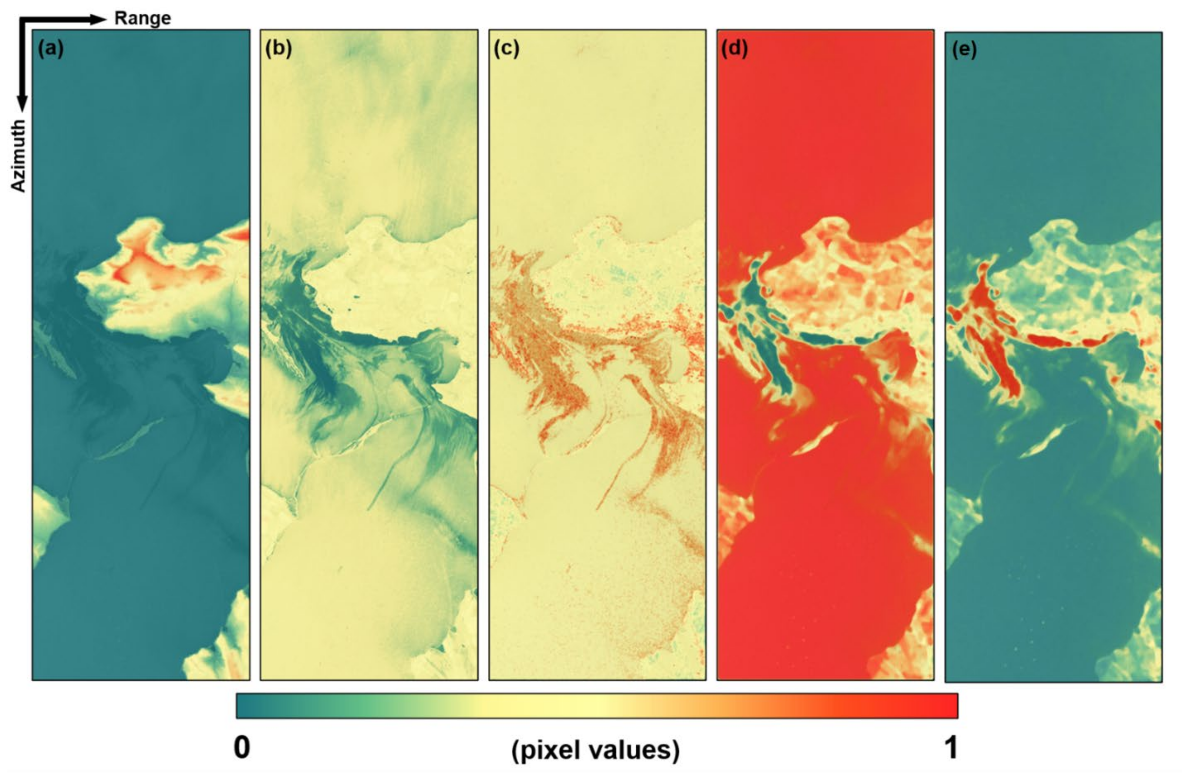
Figure 4 shows the normalized input data. To train the SVM, RF, and DNN models, the input data including (i) the shuttle radar topography mission (SRTM) digital elevation model (DEM) map, (ii) non-local mean (NL-means) filtered SAR intensity map, (iii) SAR intensity texture map, (iv) co-polarized interferometric coherence map, and (v) CPD texture map were generated from the TerraSAR-X image. The input data were normalized by min-max histogram adjustment; hence, they have a range between 0 and 1.

The SVM, RF, and DNN model parameters were estimated from the training data using the optimal hyperparameters (Table 1) in the single-pol and dual-pol groups, respectively. The training and test data of the single- and dual-pol groups were extracted from the same positions. However, the number of neurons in the input layer was three in the single-pol group while the number of neurons was five in the dual-pol group. The multi-label maps, which were respectively classified from the single-pol group by the SVM, RF, and DNN models, was seen in Figure 5. The significant difference between the three classification maps could not be found. However, the oil spill classification of the RF model was worse than the SVM and DNN models. The predicted proportions between sea surface, oil spills, ships, and land surface were approximately (1) 75.19%, 8.18%, 0.04%, and 16.58% in the DNN model, (2) 75.29%, 8.07%, 0.05%, and 16.59% in the RF model, and (3) 75.90%, 8.04%, 0.03%, and 16.03% in the SVM model, respectively. When compared to the truth data of 75.5%, 7.9%, 0.1%, and 16.6%, respectively, the oil spills were over-predicted, while the ships were under-predicted, especially for the SVM model, in which the classification performance for the ships was the worst.

Figure 6 represents the multi-label classification maps magnified from Figure 5 using the boxes A to D of Figure 3. As shown in Figure 6c,i,l, the ship pixels were not classified well in the SVM model. Common in the three model results, oil spills were not well detected in areas with relatively high NL-mean filtering intensity maps. The oil spills were not well classified in the RF model. The oil spill pixels classified by RF were noisy as shown in Figure 6b,e,h. This pattern can be found in the false alarms of oil spill lookalikes (Figure 6h). The result indicates that the input data in the single-pol group does not have enough information to classify oil spills and its lookalikes using the RF model. In addition, the misclassification of the oil spill lookalikes was found in all the models as seen in Figure 6g–i. The lakes in the land were misclassified as oil spills as seen in Figure 6d–f and the sea surface was misclassified as oil spills as shown in Figure 6g–i. The classification of the ships and land surface was performed well in the DNN and RF models (Figure 6a,b,d,e) when compared to the SVM model (Figure 6c,f). In the SVM classification, we can find that several land surfaces were misclassified as sea surfaces (Figure 6f).

By adding co-polarized coherence and CPD texture map as input data, we can determine if the classified maps become clearer compared to the single-pol group (Figure 7). The improvement on oil spill classification performance in the DNN and RF models can be determined by visual analysis (Figure 7a,b). The noisy false positive pattern of RF was remarkably reduced as shown in Figure 7b. In the SVM model, the false negative of land surface was reduced, but the false positive of land surface increased as shown in Figure 7c. The predicted proportions between sea surface, oil spills, ships, and land surface were approximately (1) 75.64%, 7.71%, 0.04%, and 16.60% in the DNN model, (2) 75.98%, 7.37%, 0.05%, and 16.60% in the RF model, and (3) 76.06%, 7.02%, 0.06%, and 16.87% in the SVM model, respectively. When compared to the result from the single-pol group, the prediction proportions of oil spills decreased, and land surfaces increased.

Figure 8 represents the multi-label classification maps magnified from Figure 7 using the boxes A to D of Figure 2. In the oil spill classification maps of DNN (Figure 8a,d,g) and RF (Figure 8b,e,h), a detailed oil spill distribution may be classified better than the single-pol group. The classification quality of the linear-shaped oil spills has been improved as seen in Figure 8g,h. The false positive of oil spill lookalikes was reduced in the DNN and RF models (see Figure 8g,h). Conversely, the oil spill mapping performance of SVM was degraded versus the single-pol group (see Figure 8c,f,i). Several oil spill areas were misclassified as the land surface class by SVM. The true positive of linear-shaped oil spills was reduced as well. In addition, the false positive of oil spill lookalikes was similar to the SVM result in the single-pol group. The ship pixels were more clearly predicted in the dual-pol group as seen in Figure 8a–c,g–l, when compared to the single-pol group, as shown in Figure 6a–c,g–l. In the DNN result, however, several pixels of nearby ships were misclassified as the land surface class (Figure 8a,g,j). The false positive of ships also increased in the SVM model as seen in Figure 8l.

A quantitative analysis was performed to assess the effect of dual-polarized SAR data on improving pixel-wise target classification performance of the data mining approach.

Table 2. Performance evaluation of the single- and dual-pol groups using precision, recall, false alarm, f1-score, and mean f1-score.

Input	Model	Hyperparameters	Precision	Recall	F1-Score	Mean F1-Score
Single-pol. group	DNN	Sea surface	0.976	0.978	0.977	0.889
		Oil	0.826	0.815	0.821
		Ship	0.894	0.681	0.773
		Land	0.987	0.984	0.986
	RF	Sea surface	0.973	0.977	0.975	0.882
		Oil	0.811	0.786	0.799
		Ship	0.831	0.718	0.770
		Land	0.987	0.984	0.986
	SVM	Sea surface	0.968	0.980	0.974	0.822
		Oil	0.825	0.800	0.812
		Ship	0.758	0.410	0.532
		Land	0.989	0.953	0.971
Dual-pol. group	DNN	Sea surface	0.980	0.982	0.981	0.898
		Oil	0.842	0.828	0.835
		Ship	0.892	0.704	0.787
		Land	0.990	0.988	0.989
	RF	Sea surface	0.979	0.986	0.983	0.908
		Oil	0.875	0.819	0.846
		Ship	0.862	0.762	0.809
		Land	0.993	0.991	0.992
	SVM	Sea surface	0.973	0.980	0.976	0.852
		Oil	0.825	0.738	0.779
		Ship	0.641	0.715	0.676
		Land	0.970	0.984	0.977

summarizes the performance evaluation scores of the single- and dual-pol groups, which are the precision, recall, f1-score, and mean f1-score. Every score was calculated by comparing ground truth and prediction results using the test data. The f1-score, which is a harmonic average of precision and recall, can give us a quantitative performance for the imbalanced class case. The best f1-scores of sea surface, oil spill, ship, and land classes can be found at the RF model in the dual-pol group. The best f1-scores were about 0.983, 0.846, 0.809, and 0.992 in the sea surface, oil spills, ships, and land surface, respectively, while the worst f1-scores were approximately 0.974, 0.779, 0.532, and 0.970, respectively. The ship classification performance was particularly low due to the data imbalance problem. When comparing the same model trained from the single- and dual-pol groups, the dual-pol group increased all the f1-scores except the oil spill classification performance of SVM, and the classification performance of the ships in the SVM model showed the largest improvement of about 0.14. The f1-scores in the RF model improved by about 0.048 and 0.039 in oil spills and ships, respectively. The improvement was relatively, high although it was lower than the performance improvement of the ships in SVM. The oil spill classification degraded from 0.812 to 0.779 in the SVM model. The mean f1-scores of DNN, RF, and SVM in the single-pol group were about 0.889, 0.882, and 0.822, respectively. The result from the DNN model showed the best performance in the single-pol group. The mean f1-scores of the ANN, RF, and SVM models in the dual-pol group were about 0.898, 0.908, and 0.852, respectively. The RF model showed the best performance in the dual-pol group. The mean f1-scores in the dual-pol group were higher than the single-pol group. The RF model showed the highest improvement of 0.0251, while the lowest improvement of 0.0089 could be found at DNN. This result indicates that the dual-pol SAR data may enhance the performance of the marine environment classification. However, when compared between the best model in the single- and dual-pol groups, the DNN model had the best performance (0.889) in the single-pol test while the RF model was best (0.908) in the dual-pol test. The improvement between the best model performance was about 2.1%. It may not be said that the improvements are noticeable.

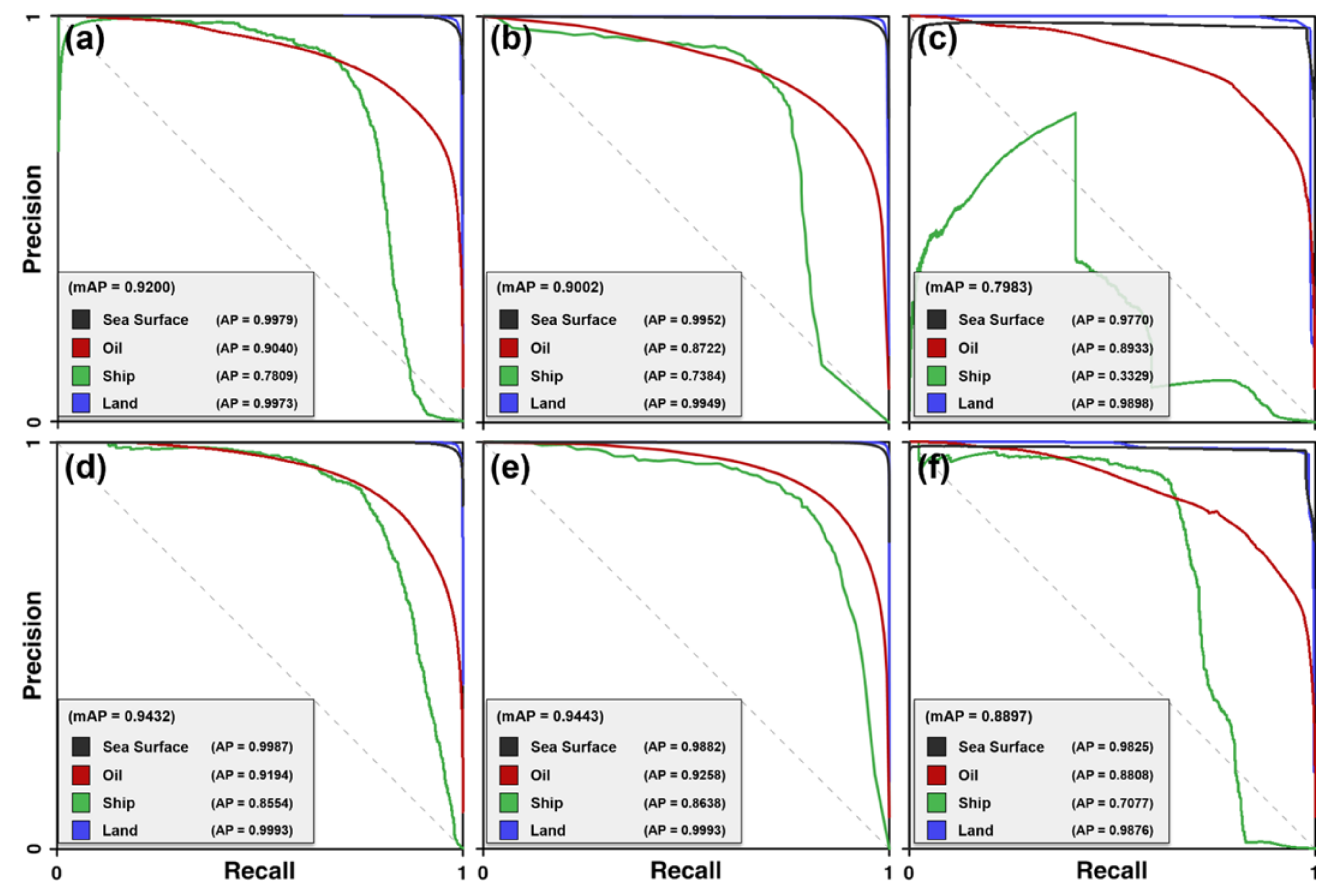
The precision-recall curve and average precision (AP) score were used for quantitatively validating the model ability to classify the multi-label classes. Figure 9 indicates the precision-recall curve and AP scores for each model, which was calculated by comparing ground truth and prediction results using the test data. The mean AP (mAP) scores of DNN were about 0.920 and 0.943 in the single- and dual-pol groups. In the single-pol group, the DNN model was equally best in the f1-score comparison. The DNN classification performance in the dual-pol group was approximately 0.023, which was better than the single-pol group. The mAP scores of RF were about 0.900 and 0.944 in the single- and dual-pol groups, respectively. In group 2, the RF model was slightly better than the DNN model. The mAP score of SVM was worse than other models due to the ship class. Since the SVM’s AP scores of ships were as low as about 0.333 and 0.708 in the single- and dual-pol groups, respectively, the mAP score of SVM was significantly reduced (Figure 9). When compared between the best classification in the single- and dual-pol groups, the DNN model had the best performance (0.920) in the single-pol test while the RF model was best (0.944) in the dual-pol test. The improvement between the best model performance was about 2.6%. This is the same as the f1-score evaluation result. Therefore, the classification performance based on mAP can be summarized as follows: (i) the dual-pol classification was slightly better than the single-pol classification in the marine environment classification; (ii) the RF model was best in the dual-pol group; (iii) the performance of DNN was similar to RF in the dual-pol group; and iv) SVM was worst in both the single- and dual-pol groups.

From the results, we can conclude the following: (i) in the case that single-pol SAR data is only available, the DNN may be the best model for the application of marine target classification; (ii) the RF model may be the best approach to classify marine targets when dual-pol SAR data is available; (iii) by using dual-pol SAR data, the improvement of the classification performance can be expected, but the improvement may not be noticeable (less than 3%); (iv) the DNN and RF models from the dual-pol SAR data can reduce the false positive of oil spill lookalikes; and (v) the RF model in the dual-pol group allows us to produce the marine environment classification map with the mean f1-score, which is higher than 0.9.

5. Conclusions

The SAR dual-polarization information can give us additional information for the marine environment classification. Thus, many studies have been conducted to classify the marine targets using the dual-polarization data. However, it is not clear whether the dual-polarized SAR data can improve the classification performance in the marine environments. In this study, we analyzed and compared the multi-label classification performance achieved from single- and dual-polarized SAR data using the DNN, RF, and SVM models. For this, five normalized maps, which are the normalized height map, non-local mean filtered SAR intensity map, SAR intensity texture map, co-polarized interferometric coherence map, and CPD texture map, were created from the TerraSAR-X SLC data, and they were used as the input data of the DNN, RF, and SVM models. To compare the classification performance estimated from the single- and dual-pol data, the input data were divided into single-pol and dual-pol groups, and the DNN, RF, and SVM models were trained by the input data of the two groups. Thus, three multi-label classification maps were created using the DNN, RF, and SVM models from the single-pol group, and the other three multi-label classification maps were generated using the DNN, RF, and SVM models from the dual-pol group.

The mean f1-score and mAP score were used for the performance comparison of the DNN, RF, and SVM models in both the single- and dual-pol groups. The mean f1-scores of the dual-pol group were better than those of the single-pol group in all classes and models. Mean f1-scores of DNN, RF, and SVM were about 0.889 and 0.898 in the single- and dual-pol groups, respectively, 0.882 and 0.908 in the single- and dual-pol groups, respectively, and 0.822 and 0.852 in the single- and dual-pol groups, respectively. The mAP scores of DNN, RF, and SVM were approximately 0.920 and 0.943, 0.900 and 0.944, and 0.798 and 0.890 in the single-pol and dual-pol group, respectively. The estimated mean f1-score and mAP scores indicate that: (i) when single-pol SAR data is only available, DNN may be the best model; (ii) the RF may be best in classifying marine targets when dual-pol SAR data is used; (iii) the improvement of the classification performance by dual-pol data can be expected, but the improvement may be not remarkable; (iv) in the consideration that dual-pol images have the expense of resolution or swath, those small improvements may not be valuable; and (v) the multi-label classification map in the marine environment may be generated with a mean f1-score of higher than 0.9.

In this study, we compared the single- and dual-pol SAR data for classifying marine targets. However, this study has three main limitations. First, the spatial characteristics of the input data could not be exploited in the model training, since the DNN, RF, and SVM models were not the patch-wise but the pixel-wise model. Thus, further study needs to be conducted using image-patch-based machine learning models such as convolutional neural network (CNN), and the performance comparison between the patch- and pixel-wise models needs to be performed. Second, the input data used in this study had the data imbalance. The proportions of all the classes were about 75.5%, 7.9%, 0.1%, and 16.6% in the sea surface, oil spills, ships, and land surface, respectively. Since the class majority was largely skewed on the sea and land pixels, the trained models were biased toward the major classes. Thus, we need to make the number of training data similar in all classes. Third, the results were derived from only a single PolSAR data, although the marine condition (such as wind speed) at the data acquisition is an important factor in marine target classification. To assess the influence of PolSAR data on the marine target classification, various case studies are additionally needed according to the different marine conditions.