
Machine Learning Algorithms for Chromophoric Dissolved Organic Matter (CDOM) Estimation Based on Landsat 8 Images


State Key Laboratory of Lake Science and Environment, Nanjing Institute of Geography and Limnology, Chinese Academy of Sciences, Nanjing 210008, China
*
Author to whom correspondence should be addressed.
Remote Sens. 2021, 13(18), 3560; https://doi.org/10.3390/rs13183560
Submission received: 12 July 2021
/
Revised: 31 August 2021
/
Accepted: 3 September 2021
/
Published: 7 September 2021
(This article belongs to the Special Issue Water Optics and Water Colour Remote Sensing 2.0)
Abstract
:Chromophoric dissolved organic matter (CDOM) is crucial in the biogeochemical cycle and carbon cycle of aquatic environments. However, in inland waters, remotely sensed estimates of CDOM remain challenging due to the low optical signal of CDOM and complex optical conditions. Therefore, developing efficient, practical and robust models to estimate CDOM absorption coefficient in inland waters is essential for successful water environment monitoring and management. We examined and improved different machine learning algorithms using extensive CDOM measurements and Landsat 8 images covering different trophic states to develop the robust CDOM estimation model. The algorithms were evaluated via 111 Landsat 8 images and 1708 field measurements covering CDOM light absorption coefficient a(254) from 2.64 to 34.04 m−1. Overall, the four machine learning algorithms achieved more than 70% accuracy for CDOM absorption coefficient estimation. Based on model training, validation and the application on Landsat 8 OLI images, we found that the Gaussian process regression (GPR) had higher stability and estimation accuracy (R2 = 0.74, mean relative error (MRE) = 22.2%) than the other models. The estimation accuracy and MRE were R2 = 0.75 and MRE = 22.5% for backpropagation (BP) neural network, R2 = 0.71 and MRE = 24.4% for random forest regression (RFR) and R2 = 0.71 and MRE = 24.4% for support vector regression (SVR). In contrast, the best three empirical models had estimation accuracies of R2 less than 0.56. The model accuracies applied to Landsat images of Lake Qiandaohu (oligo-mesotrophic state) were better than those of Lake Taihu (eutrophic state) because of the more complex optical conditions in eutrophic lakes. Therefore, machine learning algorithms have great potential for CDOM monitoring in inland waters based on large datasets. Our study demonstrates that machine learning algorithms are available to map CDOM spatial-temporal patterns in inland waters.
1. Introduction
Chromophoric dissolved organic matter (CDOM), which is also referred to as gelbstoff, gilvin or yellow matter, is widely found in natural water bodies and is a soluble and complicated mixture of organic substances consisting mainly of humic acids, fulvic acids and aromatic polymers [1]. CDOM can affect the underwater light field, and its generation, transport and transformation processes also influence the biogeochemical recycling of carbon, nitrogen and phosphorus in the water column [2,3,4,5,6].
Current research suggests that CDOM in water comes from multiple sources, including (a) allochthonous sources, which mainly include degraded organic matter from the surrounding terrestrial environment as input from terrestrial runoff, precipitation and groundwater recharge, and resuspension of sediments [7], and (b) autochthonous sources, which include the chemical degradation products of organisms from phytoplankton, macrophyte and bacteria [8]. The degradation process of CDOM mainly includes photochemical degradation and microbial degradation, which can degrade large molecules into small molecules that can be used by phytoplankton and microorganisms [9,10]. It also contributes to accelerating global warming through the emission of greenhouse gases such as carbon dioxide and methane [11]. Therefore, how to effectively monitor CDOM in aquatic environments is of great importance.
Traditional CDOM monitoring techniques are point based and measured in a laboratory. These measured CDOM absorption coefficients are accurate at specific locations, but their measurement is time-consuming and labor-intensive when covering large water areas. Therefore, remote sensing-based techniques have the advantages of a large spatial scale, long time series and traceability to map CDOM spatial-temporal patterns and are valuable tools for studying ecological and environmental changes and the global carbon cycle [12].
CDOM absorption exponentially decreases with increasing wavelength, and CDOM does not have the absorption troughs or peaks that phytochromes have; thus, CDOM primarily influences reflectance values at wavelengths below 500 nm [3,13]. In addition, for inland waters, it is more challenging to accurately estimate CDOM because its optical signal tends to overlap with or obscure the spectral signals of other optically active substances such as chlorophyll a (Chl-a) and total suspended matter (TSM) [14,15,16]. Therefore, CDOM estimation for inland and coastal waters remains challenging, with large errors compared to CDOM estimation for ocean waters [13,17].
Reviews of the literature reveal that many current scholars have developed algorithms to improve the accuracy of CDOM estimates based on remotely sensed reflectance [11,18,19,20,21,22,23,24,25,26,27,28,29,30,31,32]. Some of these algorithms are empirical methods that establish statistical relationships between the absorption coefficients of CDOM and reflectance from satellites for a single lake [33,34,35]. These empirical models using different combinations of bands to estimate CDOM in different waters are simple and easy to operate and test, but they have limited reusability and poor generalizability. Therefore, it is difficult to overcome these deficiencies because of the multicollinearity problems between the reflectivity of the individual bands [36,37,38].
The semianalytical approach to CDOM estimation is based on bio-optical radiative transfer theory, which establishes a relational function between the remotely sensed reflectance (Rrs) and the absorption and backscattering coefficients, a(λ) and b(λ), respectively. The most commonly used semianalytical approach, the quasi-analytical algorithm (QAA), was first proposed by Lee et al. and has been continuously improved [39,40,41]. Based on the QAA, the improved QAA extension (QAA-E) and QAA-CDOM algorithms have been used for CDOM estimation in various rivers, lakes, estuaries and coastal waters. [42,43,44,45,46]. The semianalytical approach improves the model generalizability; each parameter in the model has a definite physical meaning, and the accuracy and robustness of the model are further improved. However, the semianalytical approach relies on complex radiative transfer theories requiring separation of the optical composition of the water column and accurate measurement of the inherent optical properties, which is more difficult for a large number of inland water bodies with complex compositions and different trophic states [14]. Another application limitation of the QAA algorithm is that some satellite remote sensing has no corresponding spectral channels [1].
In the last decade, machine learning techniques have been increasingly used for remote sensing studies on water quality parameters relating to inland waters [47,48,49]. Machine learning algorithms can cope with nonlinearity and other complex regression problems and have greater potential and advantages for CDOM estimation than empirical methods [50]. Several authors have used machine learning regression algorithms such as artificial neural networks (ANNs), kernel ridge regression (KRR), random forest regression (RFR), Gaussian process regression (GPR), regularized linear regression (RLR) and support vector regression (SVR) to estimate CDOM absorption in lakes, thus revealing the potential of machine learning methods for future water color remote sensing [12,33,50,51,52,53,54].
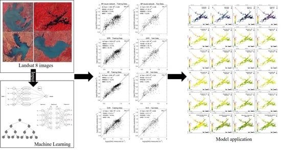
Most of the abovementioned CDOM estimation methods focus on a single lake or a few lakes in a small area and are aimed at improving the accuracy of the algorithm. In this study, we collected a large amount of CDOM light absorption coefficient data from lakes with different trophic states and applied different machine learning algorithms to Landsat 8 Operational Land Imager (OLI) imagery of lakes, with the main objective of finding the robust algorithm to estimate CDOM absorption coefficient. First, using the CDOM measured from lakes with different trophic states collected in the middle and lower reaches of the Yangtze River (YR), the upper reaches of the Huai River (RHR) and the Yunnan-Guizhou Plateau (YGP) regions and with Landsat 8 Operational Land Imager (OLI) images, we assessed the abilities of four machine learning algorithms, namely, backpropagation (BP) neural network, GPR, SVR and RFR algorithms, to estimate CDOM absorption. Second, we compared empirical algorithms (including ratio models, normalized models, and binary primary polynomial models) with machine learning algorithms using the same validation dataset. Finally, the CDOM remote sensing estimation results obtained for Lake Qiandaohu and Lake Taihu are used as examples to compare the estimation accuracy of CDOM for lakes with different trophic states across the four machine learning algorithms.
2. Datasets and Sensors
2.1. Research Area
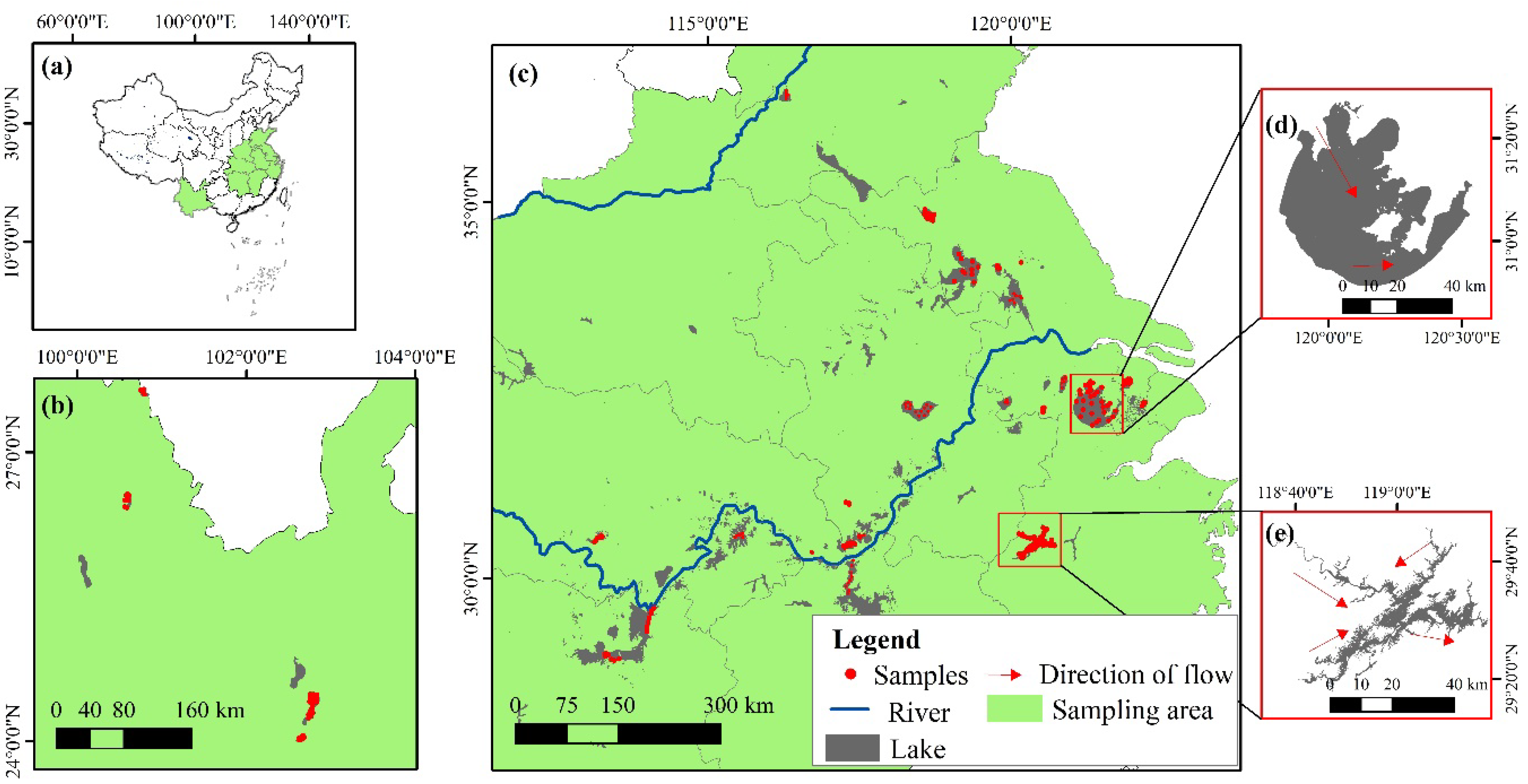
The scope of sampling in this study is spatiotemporally broad, covering mainly some lakes in the upper reaches of the Huai River, the middle and lower reaches of the Yangtze River and the Yunnan-Guizhou Plateau (Figure 1). The sampling period of Lake Taihu ranges from 2013 to 2021, and the sampling period of most lakes is mainly concentrated in 2017–2021 (Table 1). The data for Lake Qiandaohu and Lake Taihu are mostly data from routine monitoring (monthly sampling), and the data for the other lakes sampled are mostly data from winter, spring and summer bulk sampling in the lower and middle reaches of the Yangtze River and the upper reaches of the Huai River (Table 1). We chose to study the lakes in the abovementioned regions due to their different trophic states [55].
2.2. Sample Collection and Processing
To accurately measure CDOM absorption, water samples collected in situ need to be stored under dark refrigeration conditions in acid-washed polyvinyl chloride bottles and delivered back to the laboratory in a timely manner [56]. Then, water samples were filtered at low pressure, large particles and plankton cells were filtered out first using precombustion Whatman GF/F filters, and next, the samples were filtered using nitrocellulose Millipore filters with a 0.22 µm pore size. Absorption spectra of water samples filtered with 1 nm intervals in the wavelength range 200–800 nm were obtained by using a Shimadzu UV-Vis 2550 spectrophotometer, with Milli-Q water used as the blank reference [42]. Finally, the absorption coefficient at each wavelength can be calculated by Equation (1) and corrected for scattering effects by removing the absorbance at 700 nm (Equation (2)) [57].
where λ denotes wavelength, D denotes the measured absorbance, α denotes the absorption coefficient in m−1, α’ is the uncorrected absorption coefficient in m−1, and r denotes the cuvette path length in m.
In previous studies, freshwater scientists usually used the absorption coefficients at 350, 420 or 440 nm to represent CDOM in inland aquatic environments [13]. Zhang et al. (2021) [1] showed that the coefficient of determination R2 between a(350) and a(254) could reach 0.96 (p < 0.001), and we also found a stronger correlation between a(254) and the reflectance of OLI imagery. Therefore, in this study, we chose the absorption coefficient at 254 nm to characterize CDOM, which is used to develop and validate CDOM estimation models.
2.3. Remote Sensing Data Processing
Landsat 8 OLI data have a temporal resolution of 16 days and a spatial resolution of 30 m and contain four visible bands, one near infrared band (NIR) and two shortwave infrared bands. Landsat 8 imagery, which offers a new shorter wavelength blue band (ultrablue band), a narrower NIR band and a higher signal-to-noise ratio relative to Landsat 4, 5 and 7 imageries, allows for an improved ability to monitor water quality parameters in inland waters [29,31].
Nearly cloud-free imagery was downloaded from Google Earth Engine (https://code.earthengine.google.com/ (5 August 2021)), an online cloud-based geospatial processing platform dedicated to processing satellite imagery and other Earth observation data [58]. It provides a Landsat 8 OLI surface reflectance dataset after atmospheric correction using Land Surface Reflectance Code (LaSRC) software [59]. The remote sensing reflectance (Rrs) was obtained by dividing the surface reflectance by π (3.14) [59]. The Landsat 8 imagery data were matched with the measured CDOM, and the remote sensing reflectance was extracted.
The spectral information relating to marked algal bloom and aquatic vegetation was removed from the samples by setting a floating algae index (FAI) threshold (>0.01) [60], as the spectral information from algal bloom and aquatic vegetation severely masked the water light signal, which had an important effect on the training and validation of the algorithms. Therefore, the reflectance data containing marked algal bloom information were automatically removed from the imagery in later CDOM estimation, which reduced the algal spectral noise and improved the algorithm accuracy. In addition, to ensure uniformity of the water surrounding the sampling site, we tested the coefficient of variation (CV) for each band (reflectance in a 3 × 3 window centered on the sampling site, CV < 10%) [47].
2.4. Matched Data Processing
Table 1 shows a summary of the specific sampling times and sample information for the measured CDOM absorption coefficient data that were matched to Landsat 8 images. In total, 1708 data samples were matched. The time difference between the matched Landsat 8 and the measured CDOM absorption coefficient was controlled within 16 days, potentially decreasing the accuracy of our models. The matching time was suitably extended because of the long temporal resolution of Landsat 8 OLI and the small amount of matched data and because the lakes of interest were inland lakes with relatively stable CDOM [13].
3. Methods
3.1. Data Preprocessing
To improve the speed at which the gradient descent method obtains the optimal solution, the data used for model training need to be standardized [12]. In this paper, because the maximum and minimum reflectance values are difficult to determine when applied to remote sensing images, the z-score standardization method was used [61,62]. The characteristic of the z-score standardization method is that the data can be standardized to a distribution with a mean of 0 and a variance of 1, and it is not easily affected by outliers. Each input element was standardized separately according to the following formula:
where m and v denote the mean and variance, respectively, of the input elements.
3.2. BP Neural Network
Currently, the most commonly used neural network learning approach is the BP neural network algorithm. The algorithm is a multilayer feed-forward network, and the main learning process consists of a forward computation process and an error BP process. It mainly includes three structures: the input layer, the hidden layer and the output layer. Neurons at different levels are interconnected through corresponding weights. The calculation formula can be found in Equation (4) [50].
For the ith neuron, neuron i in layer is the input, the inputs are often the independent variables that are crucial to the system model, and denotes the connection weight from neuron i at layer l to neuron j at layer l + 1, which regulates the proportion of the weight of each input quantity. denotes the bias of neuron j at layer l, and is a nonlinear activation function.
Equation (5) above is the error function equation, and the actual output of the model for sample xi is denoted . is the expected output of the model. The backpropagation of error updates the network weights by reversing the output error (E) in some form layer by layer through hidden layers to input layers and assigning E to the individual neural units of each layer neuron.
In addition, the selection of other parameters, such as the training algorithm, hidden layers and iterations, also impacts the training accuracy of the model. In our case, the tansig activation function and Levenberg–Marquardt algorithm were used, and the hidden layer was set at 29 layers.
3.3. SVR
The basic idea of SVR regression is finding a regression hyperplane in a high-dimensional space so that all the data in the set are at the closest distance to that plane [63]. To use SVR to better solve the problems in regression fitting, Vapnik et al. [64] introduced an insensitive cost function () based on SVR classification, which forms the SVR model [48,50]. Given a training dataset D = {}, the SVR prediction model can be constructed as follows:
Unlike traditional regression algorithms, which typically calculate the loss based on the error between the model output and , the loss is zero if and only if is exactly the same as . SVR assumes that it can tolerate an error between and of at most ( > 0) and calculates the loss only if the prediction error is larger than . Briefly, the weights and bias could be calculated by minimizing the following function:
In Equation (8),
where denotes the loss function and C denotes the penalization parameter to penalize errors larger than ε. By introducing slack variables and , Equation (7) can be transformed into Equation (9):
The Lagrange multipliers and were used to create the Lagrange function and address the dual problem, and the final regression function is obtained as follows:
where K is a kernel function as follows:
Some typical kernel functions are available, such as the sigmoid kernel and the radial basis function kernel; the latter was used in this paper.
In this SVR model, the software package libSVR_3.24 designed by Prof. Lin Chih-Jen et al. (2021) [65] is used, and the SVR model parameters are selected using cross-validation, where gamma is 1 and cost is 2.
3.4. GPR
As a kernel-based, nonparametric probabilistic algorithm, GPR achieves a functional relationship between input and output elements by using a multivariate joint Gaussian distribution of the mean and covariance matrix of the available data.
In our GPR implementation, we use the squared exponential kernel function, which is expressed as follows:
where denotes a scale factor, B denotes the number of input elements, and denotes a dedicated parameter controlling the spreading relationship of each input element b [50].
3.5. RFR
RFR is an ensemble learning approach that constructs a large number of decision trees with no relationship between each tree during training and outputs the average of all decision tree predictions as the model prediction result [53]. First, resampling (that is, sampling with replacement) is performed using bootstrapping to generate T random training sets S1, S2, …, ST. Then, by constructing decision trees, some numbers of attributes are randomly chosen, from which the most suitable attribute is selected as the splitting node of the decision trees. After the random forest is constructed, test sample X is entered into each decision tree for calculation, and the average predicted value of all the decision trees is used as the final prediction result [66]. The advantages of RFR are that it is more resistant to noise than other methods. The model reduces the correlation between the decision trees and is less sensitive to outliers and noise, so it has better generalizability and accuracy. In our case, the random forest is set up with 100 trees and five leaf nodes.
3.6. Accuracy Assessment
In this paper, the coefficient of determination (R2), mean relative error (MRE), root mean square error (RMSE), and relative RMSE (RRMSE) between measured and estimated CDOM absorption coefficient were used to evaluate the performances of all four machine learning approaches.
where N denotes the number of data points, i denotes the ith data point, and Meas and Esti denote the CDOM absorption coefficient measurements and estimates, respectively.
3.7. Experimental Settings
In the training of the model, firstly, we used Pearson correlation analysis to determine the correlation between each OLI band and the CDOM absorption coefficient. Then, the bands with higher correlations were gradually added as inputs to the machine learning models. The results showed that the validation results were most accurate when the input element was seven bands, so in this paper we mainly use bands 1 to 7 of Landsat 8 as the input elements of the algorithms and a(254) as the output element. Although the reflectance at longer wavelengths is generally insensitive to CDOM, practical validation has shown that the performance of the algorithm can be improved by using additional longer wavelengths [36]. Among the 1708 sets of sample datasets, 1300 sets are randomly selected for model training, and 408 sets are used for model validation. To ensure the comparability between the BP neural network, GPR, RFR, and SVR algorithms, the training and validation datasets are consistent for each algorithm. Model training, statistical analysis of the parameters, error analysis, etc. are implemented in MATLAB 2019b.
4. Results
4.1. Accuracy Comparisons of Four Machine Learning Algorithms
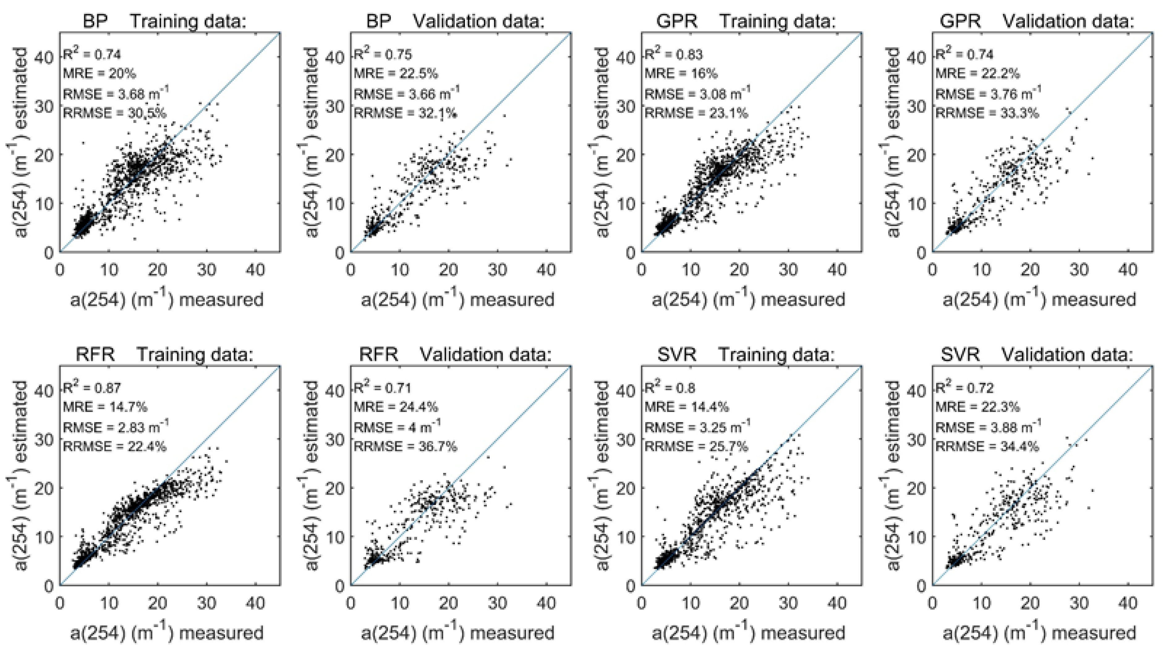
Table 2 and Figure 2 show the training and validation results of the four machine learning algorithms. The BP neural network had the highest stability in the training results (R2 = 0.74, MRE = 20% and RMSE = 3.68 m−1) and validation results (R2 = 0.75, MRE = 22.5% and RMSE = 3.66 m−1). The RFR model had the best fitting accuracy for the training data (R2 = 0.87, MRE = 14.7% and RMSE =2.83 m−1), but it had the lowest fitting accuracy for the validation data (R2 = 0.71, MRE = 24.4% and RMSE = 4.00 m−1). Therefore, the stability of the RFR model was lower than that of the other three models. The GPR (R2 = 0.74, MRE = 22.2%) and SVR (R2 = 0.72, MRE = 22.3%) models in the validation data were more accurate than the RFR model. Overall, the four machine learning algorithms achieved more than 70% accuracy for CDOM absorption coefficient estimation in the available data. The available CDOM data take very little time to run the four different algorithms, so there are no further statistics or discussion of the runtimes of the different algorithms.
4.2. Model Application for Lakes with Different Trophic States
To objectively validate the accuracy of the machine learning algorithms, the trained models were used for Landsat 8 OLI images of lakes with different trophic states, taking Lake Taihu (eutrophic state) and Lake Qiandaohu (oligo-mesotrophic state) as examples. The imageries of Lake Qiandaohu (9 August 2018) and Lake Taihu (30 July 2017) were selected for CDOM estimation and compared with the measured CDOM absorption coefficient results of the same period (within 3 days) to visually reflect the CDOM estimation capability of the different algorithms (Figure 3, Figure 4, Figure 5, Figure 6).
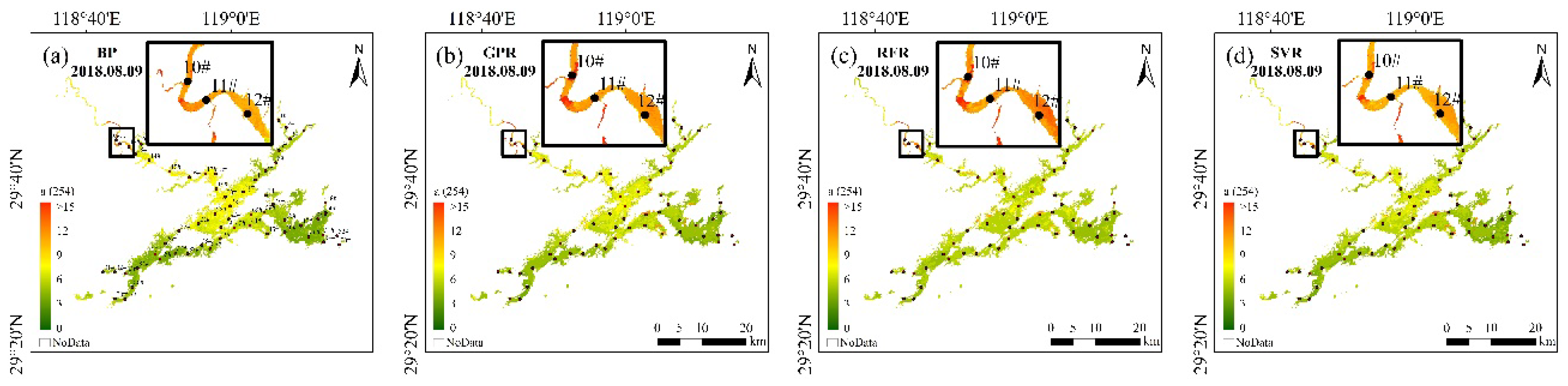
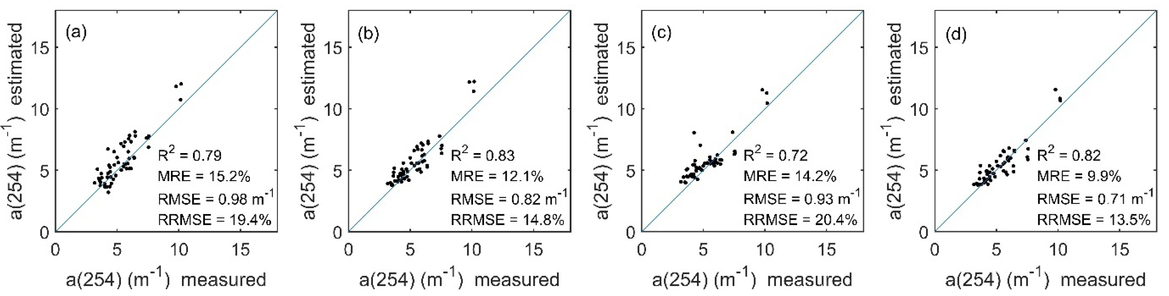
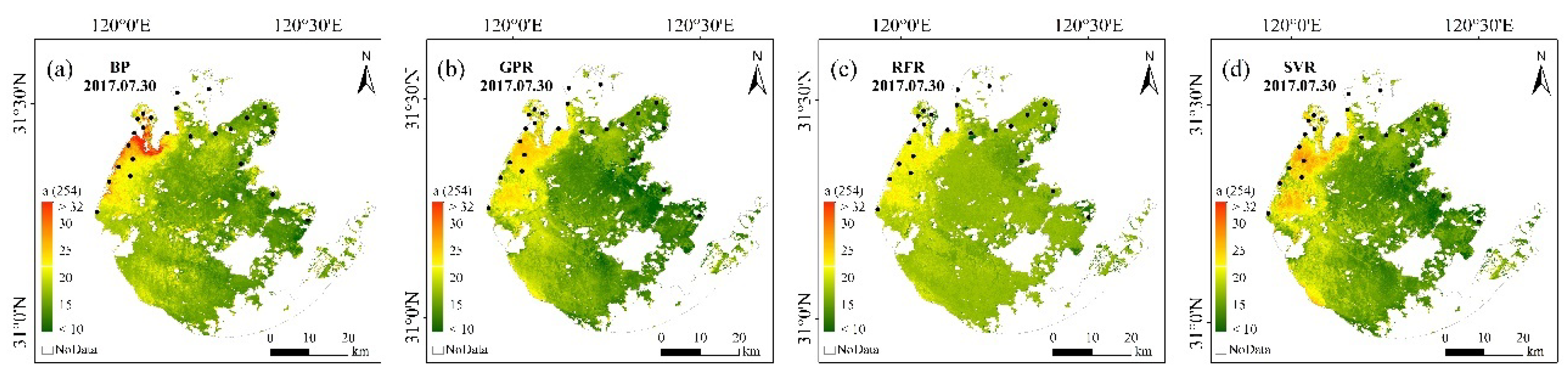
All four machine learning algorithms performed relatively well in the Lake Qiandaohu image application, with generally similar estimation results (Figure 3 and Figure 4). For the whole lake, the spatial distribution of CDOM tended to decrease from northwest to southeast. Comparison with the measured CDOM of Lake Qiandaohu showed that the estimated R2 of all four models was higher than 0.72, with the highest accuracy obtained from the GPR model with R2 = 0.83 (Figure 4). However, there is an overestimation of CDOM at the upstream boundary sampling points (e.g., 10–12#). The RFR model has a clear overestimation when the measured CDOM is less than 5.7 m−1; and a clear underestimation when the CDOM is greater than 5.7 m−1.
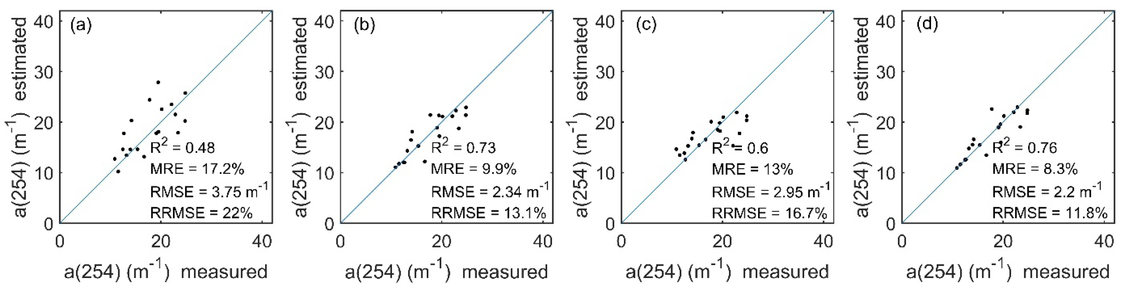
Lake Taihu had a higher level of eutrophication and higher CDOM absorption coefficient than Lake Qiandaohu. The imagery was preprocessed by FAI to automatically remove the algal bloom and aquatic vegetation information. The estimation results of the four machine learning models were generally consistent in spatial distribution, showing high values in the northwest and low values in the southeast (Figure 5). A comparison with the measured CDOM in Lake Taihu shows that the BP neural network has the lowest accuracy of 0.48, while the GPR and SVR models have better accuracy (R2 > 0.73) (Figure 6). The RFR model is consistent with the estimates at Lake Qiandaohu, with an overestimate when the measured CDOM is less than 20 m−1 and an underestimate when the CDOM is greater than 20 m−1. From the imagery, the BP neural network overestimated the northwestern part of Lake Taihu relative to the other three models. Therefore, GPR had higher stability and estimation accuracy than the other three models after comprehensively considering model training, validation and the application on Landsat 8 OLI images (Table 2 and Figure 4 and Figure 6).
By comparing the measured and estimated CDOM of the two lakes by the four machine learning algorithms, the estimation accuracy of eutrophic Lake Taihu was lower than that of oligo-mesotrophic Lake Qiandaohu. Some of the estimated results were higher than the measured CDOM, which may be due to the complexity of the Lake Qiandaohu boundary, which was influenced by the mixed pixels of the shore vegetation, resulting in high CDOM absorption coefficient. In contrast, the estimates of the GPR and RFR models were slightly lower than the measured CDOM values (>20 m−1), which could be related to the sampling sites contaminated by algal blooms, or to the small number of samples with high CDOM values in the training data. These results are also consistent with the results in RFR model, where low values were overestimated and high values were underestimated.
5. Discussion
5.1. Advantages of Machine Learning Algorithms
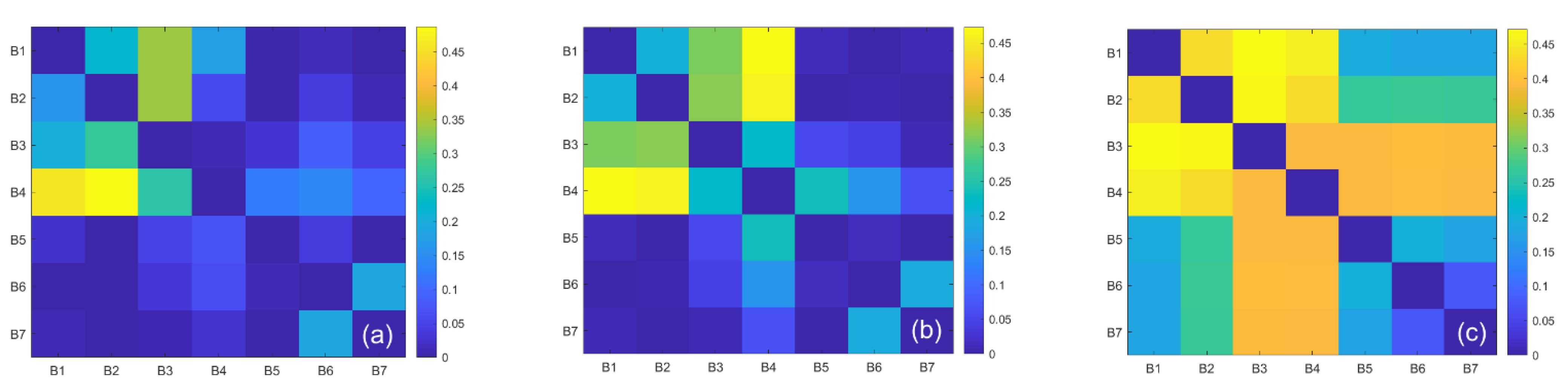
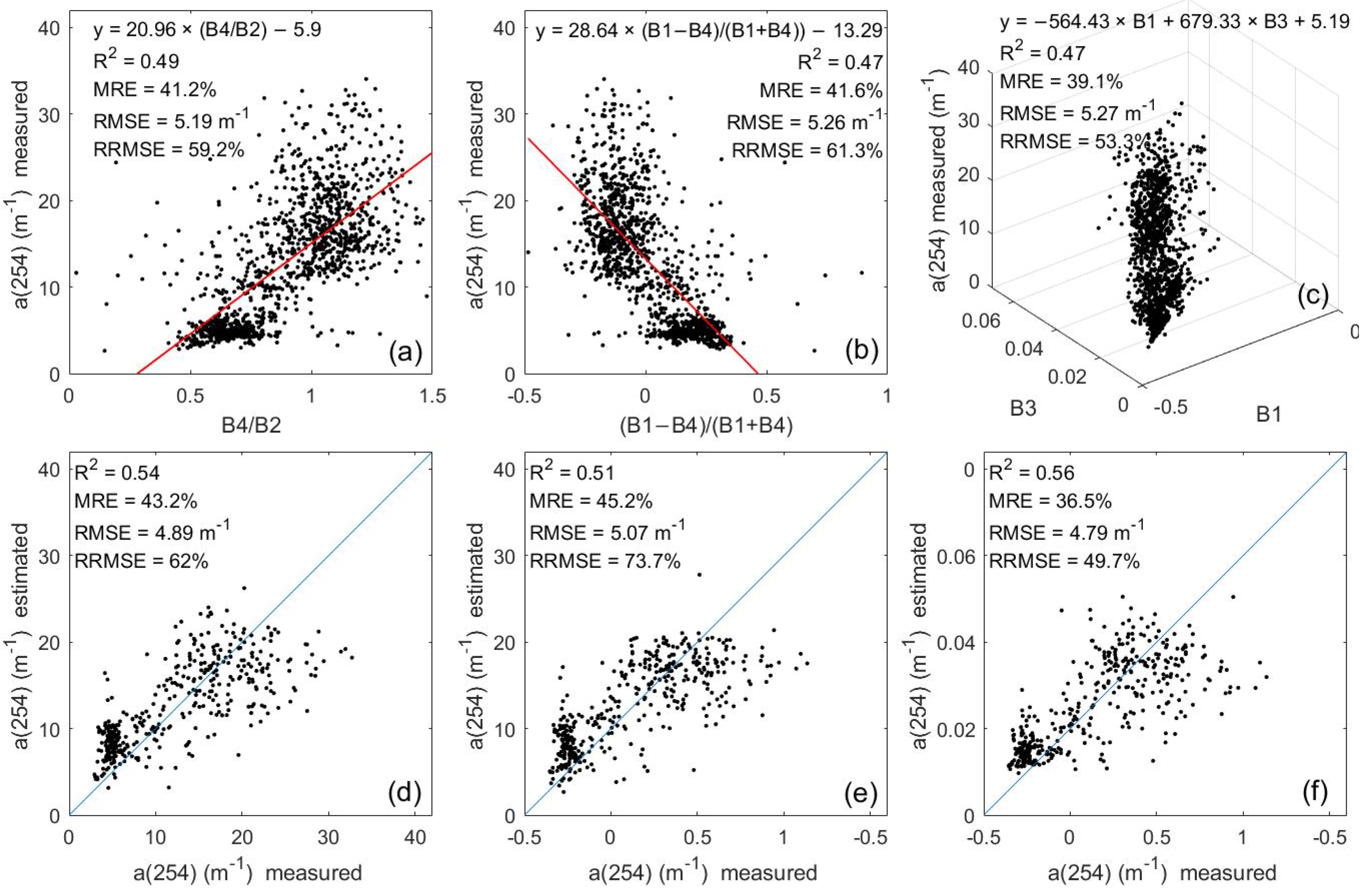
To better compare the merits of the models, we trained the commonly used empirical models (including ratio models, normalized models, binary primary polynomial models, quadratic models, etc.) based on different combinations of bands and selected the binary primary polynomial, normalized and ratio models with better accuracies for comparison (see Figure 7). The empirical algorithm with the best accuracy was also validated, and the results are shown in Figure 8. The three empirical models performed similarly, with validation accuracies of R2 = 0.54, R2 = 0.51 and R2 = 0.56, all of which were much lower than the estimation accuracies of the machine learning models. The empirical models underestimated all values of CDOM above 20 m−1. Therefore, the machine learning models (R2 > 0.71) outperformed the empirical models (Figure 8). Although it proved difficult to retrieve the CDOM in different waters, the machine learning models offered the potential for reasonable estimates of CDOM without considering the geographical location and optical complexity of the lakes.
5.2. Estimation Accuracy of the CDOM for Lakes with Different Trophic States
The estimation accuracies of CDOM in lakes with oligo-mesotrophic states were better than those in lakes with eutrophic states, perhaps due to the relatively low concentrations of optically active parameters and less interference from autochthonous and allochthonous sources of CDOM, resulting in better CDOM estimation performance in simple aquatic environmental lakes [16]. The concentration of optically active parameters (e.g., Chl-a and TSM) can also impact the optical properties of natural waters [13,16]. For example, concentration variations in Chl-a and TSM may influence the scattering and absorption characteristics of waters and the underwater light field [67]. Therefore, in the more complex optical signal of eutrophic lakes, which are affected by CDOM, TSM and Chl-a, CDOM-rich lakes have strong absorption in the blue-light band, while water-leaving optical signatures are small and CDOM has no special reflectance signals. Water color parameters with specific reflectance signals such as TSM and Chl-a dominate the reflectance spectra of complex water bodies, and the interaction between these parameters also directly affects the estimation accuracy of CDOM using remote sensing [13,15,68]. In addition, the reflectance spectrum of CDOM is very similar to that of Chl-a in blue regions, which makes it hard to separate their spectral characteristics [1,16]. Current studies on the separation of the spectrum characteristics of Chl-a, CDOM and TSM are not well established, so CDOM estimation in complex optical environments remains challenging [3].
5.3. Application of Machine Learning Modelling of Landsat Data
Based on the model comparison results, the machine learning models performed better than empirical models for Landsat 8 OLI data. Therefore, machine learning models can be extended to Landsat series data for long-term CDOM monitoring. Sensors have not been developed for inland water monitoring, but using long data series is attractive [69]. However, we cannot deny that, when applied to inland waters, the current Landsat series data are limited in terms of their temporal, spatial and spectral resolutions for CDOM estimation, especially in eutrophic lakes where various optical signals interact with each other, resulting in a lower CDOM estimation accuracy [70]. In addition, although we collected a large amount of CDOM data from lakes with different trophic states covering the complex optical properties of waters to improve the extended application and portability of the models, the machine learning models have limitations. However, the performance of a machine learning algorithm is constrained by training data characteristics. Therefore, when expanding to other regions, accuracy may be reduced [47]. Nevertheless, the potential for the remote sensing estimation of CDOM using machine learning algorithms has been identified through this extensive study; so that subsequent research could both experiment with remote sensing imagery with better temporal, spatial and spectral resolution to improve CDOM estimation accuracy in eutrophic lakes, and continuously explore the potential of other machine learning algorithms to monitor inland waters.
However, compared to TSM and Chl-a with very strong optical signal and high estimation precision [14,15,16], it is challenging to accurately estimate CDOM by satellite although we have collected a large and extensive CDOM dataset [3]. The main reasons can be attributed to two aspects. Firstly, the optical signal of CDOM is very low, generally lower than phytoplankton and nonphytoplankton particles in inland waters [71], and CDOM only absorbs and does not scatter, and its variation contributes little to reflectance [13]. Secondly, current satellite remote sensing does not have spectral channels for CDOM, just as MODIS, Sentinel and Landsat satellites have red and green spectral channels for chlorophyll and suspended matter, etc. In addition, CDOM mainly absorbs ultraviolet wavelengths below 400 nm, and none of the current satellite remote sensing has an ultraviolet channel [1,71]. Therefore, due to the characteristics of the CDOM absorption spectra, the precise estimation of the CDOM needs to be further combined with the satellites to develop suitable mathematical models.
6. Conclusions
In this study, four different machine learning algorithms were trained and validated using a large CDOM absorption coefficient dataset covering a(254) from 2.64 to 34.04 m−1 from lakes with different trophic states between 2013–2021. The results show that machine learning algorithms achieved more than 70% accuracy for CDOM estimation in the available data. When the trained model was used in lakes with different trophic states, the accuracy of CDOM for oligo-mesotrophic lakes was higher than that for eutrophic lakes, which is due to the increased optical complexity in eutrophic lakes. However, machine learning models still have great potential in eutrophic lakes, for example, the SVR model achieved an R2 of 0.76 for Lake Taihu. The spatial distribution of the CDOM results estimated for the Lake Taihu and Lake Qiandaohu showed an overall decreasing trend from the upstream to the downstream lakes, in line with the spatial variation in the measured CDOM results. Therefore, the machine learning algorithms can contribute to CDOM estimation in inland waters and have wide applications for water resource management.
Author Contributions
X.S. was responsible for data collection, processing analysis, model training and writing the manuscript; Y.Z. (Yunlin Zhang) and Y.Z. (Yibo Zhang) contributed to the design of the research and the article’s organization and revised the manuscript; K.S. contributed to the collection the remote sensing images and data analysis; Y.Z. (Yongqiang Zhou) and N.L. contributed to the collection the remote sensing images and measured CDOM data. All authors have read and agreed to the published version of the manuscript.
Funding
This work was supported by the National Natural Science Foundation of China (grants 41930760, and 41807362), Water Resource Science and Technology Project in Jiangsu Province (grant 2020057), the Provincial Natural Science Foundation of Jiangsu in China (grant BK20181104) and the Key Research Program of Frontier Sciences, Chinese Academy of Sciences (grant QYZDB-SSW- DQC016).
Acknowledgments
The authors would like to thank all the partners for their participation in field sample collection and experimental analysis. We would like to express our gratitude to the three anonymous reviewers for their critical comments and constructive suggestions.
Conflicts of Interest
The authors declare no conflict of interest.
References
- Zhang, Y.; Zhou, L.; Zhou, Y.; Zhang, L.; Yao, X.; Shi, K.; Jeppesen, E.; Yu, Q.; Zhu, W. Chromophoric dissolved organic matter in inland waters: Present knowledge and future challenges. Sci. Total Environ. 2021, 759, 143550. [Google Scholar] [CrossRef] [PubMed]
- Carder, K.L.; Steward, R.G.; Harvey, G.R.; Ortner, P.B. Marine humic and fulvi acids their effects on remote sensing of ocean chlorophyll. Limnol. Oceanogr. 1989, 34, 68–81. [Google Scholar] [CrossRef]
- Gholizadeh, M.H.; Melesse, A.M.; Reddi, L. A comprehensive review on water quality parameters estimation using remote sensing techniques. Sensors 2016, 16, 1298. [Google Scholar] [CrossRef] [Green Version]
- Hu, B.; Wang, P.; Qian, J.; Wang, C.; Zhang, N.; Cui, X. Characteristics, sources, and photobleaching of chromophoric dissolved organic matter (CDOM) in large and shallow Hongze Lake, China. J. Gt. Lakes Res. 2017, 43, 1165–1172. [Google Scholar] [CrossRef]
- Rochelle-Newall, E.J.; Fisher, T.R. Chromophoric dissolved organic matter and dissolved organic carbon in Chesapeake Bay. Mar. Chem. 2002, 77, 23–41. [Google Scholar] [CrossRef]
- Zhang, Y.; van Dijk, M.A.; Liu, M.; Zhu, G.; Qin, B. The contribution of phytoplankton degradation to chromophoric dissolved organic matter (CDOM) in eutrophic shallow lakes: Field and experimental evidence. Water Res. 2009, 43, 4685–4697. [Google Scholar] [CrossRef]
- Zhou, Y.; Yao, X.; Zhang, Y.; Shi, K.; Jeppesen, E.; Gao, G.; Zhu, G.; Qin, B. Potential rainfall-intensity and pH-driven shifts in the apparent fluorescent composition of dissolved organic matter in rainwater. Environ. Pollut. 2017, 224, 638–648. [Google Scholar] [CrossRef]
- Zhang, Y.; Liu, X.; Wang, M.; Qin, B. Compositional differences of chromophoric dissolved organic matter derived from phytoplankton and macrophytes. Org. Geochem. 2013, 55, 26–37. [Google Scholar] [CrossRef]
- Tzortziou, M.; Osburn, C.L.; Neale, P.J. Photobleaching of dissolved organic material from a tidal marsh-estuarine. Photochem. Photobiol. 2007, 83, 782–792. [Google Scholar] [CrossRef] [PubMed]
- Zhang, Y.; Liu, M.; Qin, B.; Feng, S. Photochemical degradation of chromophoric-dissolved organic matter exposed to simulated UV-B and natural solar radiation. Hydrobiologia 2009, 627, 159–168. [Google Scholar] [CrossRef]
- Al-Kharusi, E.S.; Tenenbaum, D.E.; Abdi, A.M.; Kutser, T.; Karlsson, J.; Bergstroem, A.-K.; Berggren, M. Large-scale retrieval of coloured dissolved organic matter in northern lakes using Sentinel-2 data. Remote Sens. 2020, 12, 157. [Google Scholar] [CrossRef] [Green Version]
- Keller, S.; Maier, P.M.; Riese, F.M.; Norra, S.; Holbach, A.; Borsig, N.; Wilhelms, A.; Moldaenke, C.; Zaake, A.; Hinz, S. Hyperspectral data and machine learning for estimating CDOM, chlorophyll a, diatoms, green algae and turbidity. Int. J. Environ. Res. Public Health 2018, 15, 1881. [Google Scholar] [CrossRef] [PubMed] [Green Version]
- Brezonik, P.L.; Olmanson, L.G.; Finlay, J.C.; Bauer, M.E. Factors affecting the measurement of CDOM by remote sensing of optically complex inland waters. Remote Sens. Environ. 2015, 157, 199–215. [Google Scholar] [CrossRef]
- Aurin, D.A.; Dierssen, H.M. Advantages and limitations of ocean color remote sensing in CDOM-dominated, mineral-rich coastal and estuarine waters. Remote Sens. Environ. 2012, 125, 181–197. [Google Scholar] [CrossRef]
- Menken, K.D.; Brezonik, P.L. Influence of chlorophyll and colored dissolved organic matter (CDOM) on lake reflectance spectra: Implications for measuring lake properties by remote sensing. Lake Reserv. Manag. 2006, 22, 179–190. [Google Scholar] [CrossRef] [Green Version]
- Shang, Y.; Liu, G.; Wen, Z.; Jacinthe, P.A.; Song, K.; Zhang, B.; Lyu, L.; Li, S.; Wang, X.; Yu, X. Remote estimates of CDOM using Sentinel-2 remote sensing data in reservoirs with different trophic states across China. J. Environ. Manag. 2021, 286, 112275. [Google Scholar] [CrossRef] [PubMed]
- Zhu, W.; Huang, L.; Sun, N.; Chen, J.; Pang, S. Landsat 8-observed water quality and its coupled environmental factors for urban scenery lakes: A case study of West Lake. Water Environ. Res. 2020, 92, 255–265. [Google Scholar] [CrossRef]
- Joshi, I.D.; D’Sa, E.J.; Osburn, C.L.; Bianchi, T.S.; Ko, D.S.; Oviedo-Vargas, D.; Arellano, A.R.; Ward, N.D. Assessing chromophoric dissolved organic matter (CDOM) distribution, stocks, and fluxes in Apalachicola Bay using combined field, VIIRS ocean color, and model observations. Remote Sens. Environ. 2017, 191, 359–372. [Google Scholar] [CrossRef]
- Kutser, T.; Pierson, D.C.; Tranvik, L.; Reinart, A.; Sobek, S.; Kallio, K. Using satellite remote sensing to estimate the colored dissolved organic matter absorption coefficient in lakes. Ecosystems 2005, 8, 709–720. [Google Scholar] [CrossRef]
- Mannino, A.; Novak, M.G.; Hooker, S.B.; Hyde, K.; Aurin, D. Algorithm development and validation of CDOM properties for estuarine and continental shelf waters along the northeastern U.S. coast. Remote Sens. Environ. 2014, 152, 576–602. [Google Scholar] [CrossRef]
- Shanmugam, P. New models for retrieving and partitioning the colored dissolved organic matter in the global ocean: Implications for remote sensing. Remote Sens. Environ 2011, 115, 1501–1521. [Google Scholar] [CrossRef]
- Swan, C.M.; Nelson, N.B.; Siegel, D.A.; Fields, E.A. A model for remote estimation of ultraviolet absorption by chromophoric dissolved organic matter based on the global distribution of spectral slope. Remote Sens. Environ. 2013, 136, 277–285. [Google Scholar] [CrossRef]
- Cao, F.; Tzortziou, M.; Hu, C.; Mannino, A.; Fichot, C.G.; Del Vecchio, R.; Najjar, R.G.; Novak, M. Remote sensing retrievals of colored dissolved organic matter and dissolved organic carbon dynamics in North American estuaries and their margins. Remote Sens. Environ. 2018, 205, 151–165. [Google Scholar] [CrossRef]
- Ficek, D.; Zapadka, T.; Dera, J. Remote sensing reflectance of Pomeranian lakes and the Baltic. Oceanologia 2011, 53, 959–970. [Google Scholar] [CrossRef] [Green Version]
- Griffin, C.G.; Frey, K.E.; Rogan, J.; Holmes, R.M. Spatial and interannual variability of dissolved organic matter in the Kolyma River, East Siberia, observed using satellite imagery. J. Geophys. Res.-Biogeosci. 2011, 116, 12. [Google Scholar] [CrossRef] [Green Version]
- Jiang, G.; Ma, R.; Duan, H.; Loiselle, S.A.; Xu, J.; Liu, D. Remote determination of chromophoric dissolved organic matter in lakes, China. Int. J. Digit. Earth 2013, 7, 897–915. [Google Scholar] [CrossRef]
- Kutser, T.; Pierson, D.C.; Kallio, K.Y.; Reinart, A.; Sobek, S. Mapping lake CDOM by satellite remote sensing. Remote Sens. Environ. 2005, 94, 535–540. [Google Scholar] [CrossRef]
- Mannino, A.; Russ, M.E.; Hooker, S.B. Algorithm development and validation for satellite-derived distributions of DOC and CDOM in the US Middle Atlantic Bight. J. Geophys. Res.-Ocean. 2008, 113, 19. [Google Scholar] [CrossRef]
- Olmanson, L.G.; Brezonik, P.L.; Finlay, J.C.; Bauer, M.E. Comparison of Landsat 8 and Landsat 7 for regional measurements of CDOM and water clarity in lakes. Remote Sens. Environ. 2016, 185, 119–128. [Google Scholar] [CrossRef]
- Toming, K.; Kutser, T.; Laas, A.; Sepp, M.; Paavel, B.; Noges, T. First experiences in mapping lake water quality parameters with Sentinel-2 MSI imagery. Remote Sens. 2016, 8, 640. [Google Scholar] [CrossRef] [Green Version]
- Watanabe, F.; Alcântara, E.; Curtarelli, M.; Kampel, M.; Stech, J. Landsat-based remote sensing of the colored dissolved organic matter absorption coefficient in a tropical oligotrophic reservoir. Remote Sens. Appl. Soc. Environ. 2018, 9, 82–90. [Google Scholar] [CrossRef]
- Yu, Q.; Tian, Y.Q.; Zheng, Y.; Zhu, W.; Chen, J. Monitoring seasonal variations of colored dissolved organic matter for the Saginaw River based on Landsat-8 data. Water Supply 2019, 19, 274–281. [Google Scholar]
- Kishino, M.; Tanaka, A.; Ishizaka, J. Retrieval of Chlorophyll a, suspended solids, and colored dissolved organic matter in Tokyo Bay using ASTER data. Remote Sens. Environ. 2005, 99, 66–74. [Google Scholar] [CrossRef]
- Xu, J.; Fang, C.; Gao, D.; Zhang, H.; Gao, C.; Xu, Z.; Wang, Y. Optical models for remote sensing of chromophoric dissolved organic matter (CDOM) absorption in Poyang Lake. ISPRS J. Photogramm. Remote Sens. 2018, 142, 124–136. [Google Scholar] [CrossRef]
- Morel, A.; Gentili, B. A simple band ratio technique to quantify the colored dissolved and detrital organic material from ocean color remotely sensed data. Remote Sens. Environ. 2009, 113, 998–1011. [Google Scholar] [CrossRef]
- Zhu, W.; Yu, Q.; Tian, Y.Q.; Becker, B.L.; Zheng, T.; Carrick, H.J. An assessment of remote sensing algorithms for colored dissolved organic matter in complex freshwater environments. Remote Sens. Environ. 2014, 140, 766–778. [Google Scholar] [CrossRef]
- Chen, J.; de Hoogh, K.; Gulliver, J.; Hoffmann, B.; Hertel, O.; Ketzel, M.; Bauwelinck, M.; van Donkelaar, A.; Hvidtfeldt, U.A.; Katsouyanni, K.; et al. A comparison of linear regression, regularization, and machine learning algorithms to develop Europe-wide spatial models of fine particles and nitrogen dioxide. Environ. Int. 2019, 130, 104934. [Google Scholar] [CrossRef]
- Griffin, C.G.; McClelland, J.W.; Frey, K.E.; Fiske, G.; Holmes, R.M. Quantifying CDOM and DOC in major Arctic rivers during ice-free conditions using Landsat TM and ETM+ data. Remote Sens. Environ. 2018, 209, 395–409. [Google Scholar] [CrossRef]
- Lee, Z.; Carder, K.L.; Arnone, R.A. Deriving inherent optical properties from water colora multiband quasi-analytical algorithm for opticallydeep waters. Appl. Opt. 2002, 41, 5755–5772. [Google Scholar] [CrossRef]
- Lee, Z.; Weidemann, A.; Kindle, J.; Arnone, R.; Carder, K.L.; Davis, C. Euphotic zone depth: Its derivation and implication to ocean-color remote sensing. J. Geophys. Res. 2007, 112, C03009. [Google Scholar] [CrossRef] [Green Version]
- Lee, Z.; Lubac, B.; Werdell, J.; Arnone, R. An Update of the Quasi-Analytical Algorithm (QAA_v5). Available online: http://www.ioccg.org/groups/Software_OCA/QAA_v5.pdf (accessed on 12 July 2021).
- Li, J.; Yu, Q.; Tian, Y.Q.; Becker, B.L.; Siqueira, P.; Torbick, N. Spatio-temporal variations of CDOM in shallow inland waters from a semi-analytical inversion of Landsat-8. Remote Sens. Environ. 2018, 218, 189–200. [Google Scholar] [CrossRef]
- Zhu, W.; Yu, Q.; Tian, Y.Q.; Chen, R.F.; Gardner, G.B. Estimation of chromophoric dissolved organic matter in the Mississippi and Atchafalaya river plume regions using above-surface hyperspectral remote sensing. J. Geophys. Res. 2011, 116, C02011. [Google Scholar] [CrossRef]
- Zhu, W.; Yu, Q. Inversion of chromophoric dissolved organic matter from EO-1 Hyperion imagery for turbid estuarine and coastal waters. IEEE Trans. Geosci. Remote Sens. 2013, 51, 3286–3298. [Google Scholar] [CrossRef]
- Zhu, W.; Yu, Q.; Tian, Y.Q. Uncertainty analysis of remote sensing of colored dissolved organic matter: Evaluations and comparisons for three rivers in North America. ISPRS J. Photogramm. Remote Sens. 2013, 84, 12–22. [Google Scholar] [CrossRef]
- Zhu, W.; Tian, Y.Q.; Yu, Q.; Becker, B.L. Using Hyperion imagery to monitor the spatial and temporal distribution of colored dissolved organic matter in estuarine and coastal regions. Remote Sens. Environ. 2013, 134, 342–354. [Google Scholar] [CrossRef]
- Cao, Z.; Ma, R.; Duan, H.; Pahlevan, N.; Melack, J.; Shen, M.; Xue, K. A machine learning approach to estimate chlorophyll-a from Landsat-8 measurements in inland lakes. Remote Sens. Environ. 2020, 248, 111974. [Google Scholar] [CrossRef]
- Guo, H.; Huang, J.J.; Chen, B.; Guo, X.; Singh, V.P. A machine learning-based strategy for estimating non-optically active water quality parameters using Sentinel-2 imagery. Int. J. Remote Sens. 2020, 42, 1841–1866. [Google Scholar] [CrossRef]
- Pahlevan, N.; Smith, B.; Schalles, J.; Binding, C.; Cao, Z.; Ma, R.; Alikas, K.; Kangro, K.; Gurlin, D.; Hà, N.; et al. Seamless retrievals of chlorophyll-a from Sentinel-2 (MSI) and Sentinel-3 (OLCI) in inland and coastal waters: A machine-learning approach. Remote Sens. Environ. 2020, 240, 111604. [Google Scholar] [CrossRef]
- Verrelst, J.; Muñoz, J.; Alonso, L.; Delegido, J.; Rivera, J.P.; Camps-Valls, G.; Moreno, J. Machine learning regression algorithms for biophysical parameter retrieval: Opportunities for Sentinel-2 and -3. Remote Sens. Environ. 2012, 118, 127–139. [Google Scholar] [CrossRef]
- Blix, K.; Pálffy, K.; Tóth, V.; Eltoft, T. Remote sensing of water quality parameters over Lake Balaton by using Sentinel-3 OLCI. Water 2018, 10, 1428. [Google Scholar] [CrossRef] [Green Version]
- Nazeer, M.; Alsahli, M.; Waqas, A. Evaluation of empirical and machine learning algorithms for estimation of coastal water quality parameters. ISPRS Int. J. Geo-Inf. 2017, 6, 360. [Google Scholar] [CrossRef] [Green Version]
- Ruescas, A.; Hieronymi, M.; Mateo-Garcia, G.; Koponen, S.; Kallio, K.; Camps-Valls, G. Machine learning regression approaches for colored dissolved organic matter (CDOM) retrieval with S2-MSI and S3-OLCI simulated data. Remote Sens. 2018, 10, 786. [Google Scholar] [CrossRef] [Green Version]
- Zhao, J.; Cao, W.; Xu, Z.; Ai, B.; Yang, Y.; Jin, G.; Wang, G.; Zhou, W.; Chen, Y.; Chen, H.; et al. Estimating CDOM concentration in highly turbid estuarine coastal waters. J. Geophys. Res. Ocean. 2018, 123, 5856–5873. [Google Scholar] [CrossRef]
- Zhang, Y.; Yin, Y.; Zhang, E.; Zhu, G.; Liu, M.; Feng, L.; Qin, B.; Liu, X. Spectral attenuation of ultraviolet and visible radiation in lakes in the Yunnan Plateau, and the middle and lower reaches of the Yangtze River, China. Photochem. Photobiol. Sci. 2011, 10, 469–482. [Google Scholar] [CrossRef]
- Zhou, Y.; Zhang, Y.; Shi, K.; Niu, C.; Liu, X.; Duan, H. Lake Taihu, a large, shallow and eutrophic aquatic ecosystem in China serves as a sink for chromophoric dissolved organic matter. J. Gt. Lakes Res. 2015, 41, 597–606. [Google Scholar] [CrossRef]
- Zhang, Y.; Zhang, B.; Ma, R.; Feng, S.; Le, C. Optically active substances and their contributions to the underwater light climate in Lake Taihu, a large shallow lake in China. Fundam. Appl. Limnol. 2007, 170, 11–19. [Google Scholar] [CrossRef]
- Gorelick, N.; Hancher, M.; Dixon, M.; Ilyushchenko, S.; Thau, D.; Moore, R. Google Earth Engine: Planetary-scale geospatial analysis for everyone. Remote Sens. Environ. 2017, 202, 18–27. [Google Scholar] [CrossRef]
- Zhang, Y.; Zhang, Y.; Shi, K.; Zhou, Y.; Li, N. Remote sensing estimation of water clarity for various lakes in China. Water Res. 2021, 192, 116844. [Google Scholar] [CrossRef] [PubMed]
- Hu, C. A novel ocean color index to detect floating algae in the global oceans. Remote Sens. Environ. 2009, 113, 2118–2129. [Google Scholar] [CrossRef]
- Han, J.; Kamber, M.; Pei, J. Data Mining: Concepts and Techniques; Elsevier Inc.: Amsterdam, The Netherlands, 2012. [Google Scholar]
- Gibert, K.; Sànchez–Marrè, M.; Izquierdo, J.; Gibert, K. A survey on pre-processing techniques: Relevant issues in the context of environmental data mining. AI Commun. 2016, 29, 627–663. [Google Scholar] [CrossRef] [Green Version]
- Smola, A.J.; Scholkopf, B. A tutorial on support vector regression. Statistics and computing. Stat. Comput. 2004, 14, 199–222. [Google Scholar] [CrossRef] [Green Version]
- Vapnik, V.N. The Nature of Statistical Learning Theory; Springer: New York, NY, USA, 1995. [Google Scholar]
- Chang, C.-C.; Lin, C.-J. LIBSVM: A Library for Support Vector Machines. ACM Trans. Intell. Syst. Technol. 2021, 2, 1–27. [Google Scholar] [CrossRef]
- Breiman, L. Random Forests. Mach. Learn. 2001, 45, 5–32. [Google Scholar] [CrossRef] [Green Version]
- Shi, K.; Zhang, Y.; Song, K.; Liu, M.; Zhou, Y.; Zhang, Y.; Li, Y.; Zhu, G.; Qin, B. A semi-analytical approach for remote sensing of trophic state in inland waters: Bio-optical mechanism and application. Remote Sens. Environ. 2019, 232, 11349. [Google Scholar] [CrossRef]
- Brezonik, P.; Menken, K.D.; Bauer, M. Landsat-based remote sensing of lake water quality characteristics, including Chlorophyll and colored dissolved organic matter (CDOM). Lake Reserv. Manag. 2005, 21, 373–382. [Google Scholar] [CrossRef]
- Kutser, T. The possibility of using the Landsat image archive for monitoring long time trends in coloured dissolved organic matter concentration in lake waters. Remote Sens. Environ. 2012, 123, 334–338. [Google Scholar] [CrossRef]
- Palmer, S.C.J.; Kutser, T.; Hunter, P.D. Remote sensing of inland waters: Challenges, progress and future directions. Remote Sens. Environ. 2015, 157, 1–8. [Google Scholar] [CrossRef] [Green Version]
- Zhang, Y.; Zhang, B.; Wang, X.; Li, J.; Feng, S.; Zhao, Q.; Liu, M.; Qin, B. A study of absorption characteristics of chromophoric dissolved organic matter and particles in Lake Taihu, China. Hydrobiologia 2007, 592, 105–120. [Google Scholar] [CrossRef]
Figure 1.
Distribution of the sampling sites and examples of lakes with different trophic states: (a) location of sampling area in China; (b) sampled lakes in the Yunnan-Guizhou Plateau; (c) sampled lakes in the upper reaches of the Huai River, the middle and lower reaches of the Yangtze River; (d) Lake Taihu (eutrophic states) and (e) Lake Qiandaohu (oligo-mesotrophic states).

Figure 2.
Performance evaluation of the a(254) retrievals using the machine learning algorithms (i.e., the BP neural network, GPR, RFR and SVR models); training results are shown on the left, and validation results are shown on the right.
Figure 2.
Performance evaluation of the a(254) retrievals using the machine learning algorithms (i.e., the BP neural network, GPR, RFR and SVR models); training results are shown on the left, and validation results are shown on the right.

Figure 3.
CDOM values produced by the OLI imagery using the different machine learning models in Lake Qiandaohu (9 August 2018); the black dots show the locations of the in situ sampling points. (a–d) represent BP, GPR, RFR and SVR models respectively.
Figure 3.
CDOM values produced by the OLI imagery using the different machine learning models in Lake Qiandaohu (9 August 2018); the black dots show the locations of the in situ sampling points. (a–d) represent BP, GPR, RFR and SVR models respectively.

Figure 4.
Comparison between the measured and OLI-derived CDOM in Lake Qiandaohu. (a–d) represent BP, GPR, RFR and SVR models respectively.
Figure 4.
Comparison between the measured and OLI-derived CDOM in Lake Qiandaohu. (a–d) represent BP, GPR, RFR and SVR models respectively.

Figure 5.
CDOM values produced by the OLI imagery using the different machine learning models in Lake Taihu (30 July 2017); the black dots show the locations of the in situ sampling points. (a–d) represent BP, GPR, RFR and SVR models respectively.
Figure 5.
CDOM values produced by the OLI imagery using the different machine learning models in Lake Taihu (30 July 2017); the black dots show the locations of the in situ sampling points. (a–d) represent BP, GPR, RFR and SVR models respectively.

Figure 6.
Comparison between the measured and OLI-derived CDOM in Lake Taihu. (a–d) represent BP, GPR, RFR and SVR models respectively.
Figure 6.
Comparison between the measured and OLI-derived CDOM in Lake Taihu. (a–d) represent BP, GPR, RFR and SVR models respectively.

Figure 7.
Training results (R2) obtained for the Landsat 8 images using empirical predictive algorithms of different band combinations. (a) Band ratio method (i.e., y = a × (Bi/Bj) + c), (b) normalization method (i.e., y = a × ((Bi − Bj)/(Bi + Bj)) + c), and (c) binary first-order polynomial method (i.e., y = a × Bi + b × Bj + c), where a and b are slopes, c is an intercept, and Bi and Bj are the Landsat 8 bands.

Figure 8.
Training and validation results (R2, RME, RMSE and RRMSE) obtained using empirical predictive algorithms. (a–c) are the training results for y = a × (Bi/Bj) + c), y = a × ((Bi − Bj)/(Bi + Bj)) + c and y = a × Bi + b × Bj + c, respectively, and (d–f) are the validation results.
Figure 8.
Training and validation results (R2, RME, RMSE and RRMSE) obtained using empirical predictive algorithms. (a–c) are the training results for y = a × (Bi/Bj) + c), y = a × ((Bi − Bj)/(Bi + Bj)) + c and y = a × Bi + b × Bj + c, respectively, and (d–f) are the validation results.


Table 1.
Results of matching the Landsat 8 cloud-free imagery with the aCDOM(254) measured in situ in lakes sampled from April 2013 to May 2021.
Table 1.
Results of matching the Landsat 8 cloud-free imagery with the aCDOM(254) measured in situ in lakes sampled from April 2013 to May 2021.
| Area | Lakes | Match-Up Dates | No. of Match-Ups | aCDOM(254) (m−1) | ||
|---|---|---|---|---|---|---|
| Min | Max | Ave | ||||
| YR | Lake Baima | 17 January 2018 and 19 April 2018 | 5 | 20.18 | 22.8 | 21.43 |
| Changhu Lake | 12 January 2018 and 20 April 2018 | 8 | 11.57 | 18.16 | 15.19 | |
| Lake Chaohu | 24 April 2018 and 24 July 2018 | 25 | 13.89 | 24.73 | 17.70 | |
| Dianshan Lake | 19 July 2018 | 3 | 19.62 | 20.82 | 20.03 | |
| Dongting Lake | 21 July 2018 | 14 | 8.94 | 12.86 | 11.76 | |
| Lake Gehu | 26 April 2018 and 19 July 2018 | 7 | 14.52 | 20.36 | 17.06 | |
| Huating Lake | 20 July 2018 | 1 | 7.75 | 7.75 | 7.75 | |
| Huangda Lake | 21 January 2018 and 20 July 2018 | 4 | 14.85 | 18.06 | 16.75 | |
| Liangzi Lake | 17 January 2018 and 13 July 2018 | 14 | 6.80 | 16.84 | 11.14 | |
| Longgan Lake | 19 July 2018 | 8 | 21.35 | 31.84 | 25.46 | |
| Poyang Lake | 15 July 2018 | 8 | 13.62 | 18.12 | 15.21 | |
| Lake Qiandaohu | 19 August 2016; 8 August 2017 and 27 December 2017; 2 April 2018, 1 August 2018, 7 August 2018, 9 October 2018 and 6 November 2018; 1 April 2019 and 5 June 2019; 27 April 2020, 21 July 2020, 26 August 2020, 23 September 2020 and 23 December 2020; 27 January 2021 and 24 March 2021 | 649 | 2.64 | 32.77 | 7.81 | |
| Lake Taihu | 10 April 2013, 17 June 2013, 8 July 2013, 10 July 2013, 17 July 2013, 22 July 2013, 29 July 2013, 20 August 2013 and 14 October 2013; 22 July 2014 and 8 October 2014; 20 May 2015, 29 July 2015, 1 September 2015, 8 September 2015 and 14 October 2015; 26 July 2016, 16 August 2016, 30 August 2016, and 21 September 2016; 11 May 2017, 29 May 2017, 19 July 2017, 2 August 2017, 15 August 2017 and 18 September 2017; 3 June 2019, 29 July 2019, 13 August 2019, 14 August 2019 and 9 September 2019 | 433 | 9.55 | 34.04 | 19 | |
| Lake Tianmuhu | 28 January 2016, 29 February 2016, 22 March 2016, 18 April 2016, 24 May 2016, 20 July 2016, 25 August 2016 and 15 December 2016; 16 May 2017, 15 July 2017, 19 September 2017, 20 November 2017 and 18 December 2017; 15 January 2018, 5 February 2018, 19 March 2018, 17 April 2018, 22 May 2018 and 12 June 2018; 15 April 2019, 13 August 2019, 18 September 2019 and 18 October 2019; 13 January 2020, 14 October 2020, 18 November 2020 and 14 December 2020; 14 January 2021 and 18 May 2021 | 150 | 8.23 | 23.7 | 11.44 | |
| Lake Wushan | 18 January 2018 and 14 July 2018 | 6 | 21.05 | 32.77 | 27.21 | |
| Yangcheng Lake | 18 July 2018 | 4 | 20.23 | 21.85 | 21.00 | |
| RHR | Lake Dongping | 9 May 2018 | 2 | 24.61 | 24.78 | 24.70 |
| Lake Hongze | 28 November 2017; 9 June 2018, 1 August 2018 and 28 September 2018; 23 January 2019, 24 May 2019, 24 July 2019 and 25 September 2019; 14 January 2020, 28 March 2020, 30 April 2020, 22 May 2020, 19 June 2020, 26 September 2020, 21 October 2020, 24 November 2020 and 22 December 2020; 2 March, 7 April 2021 and 2 June 2021 | 188 | 9 | 31.32 | 18.72 | |
| Gaoyou Lake | 18 January 2018, 20 April 2018 and 15 July 2018 | 21 | 12.85 | 28.62 | 19.51 | |
| Lake Luoma | 7 June 2018; 24 January 2019, 26 February, 27 June 2019, 25 July 2019 and 29 August 2019; 27 April 2020, 21 May 2020, 31 August 2020, 19 October 2020 and 21 December 2020; 27 January 2021 | 123 | 9.23 | 28.21 | 17.27 | |
| YGP | Chenghai Lake | 10 December 2016 | 6 | 9.49 | 24.77 | 16.39 |
| Lake Fuxian | 7 November 2017 and 16 January 2018 | 25 | 2.83 | 5.84 | 3.61 | |
| Lugu Lake | 5 April 2018 | 4 | 2.64 | 3.94 | 3.14 | |
| All lakes | 24 in total | 1708 | 2.64 | 34.04 | 12.72 | |
Table 2.
Training and validation results (R2, MRE, RMSE and RRMSE) obtained for a(254) using machine learning algorithms.
Table 2.
Training and validation results (R2, MRE, RMSE and RRMSE) obtained for a(254) using machine learning algorithms.
| Training Data | Validation Data | |||||||
|---|---|---|---|---|---|---|---|---|
| R2 | MRE (%) | RMSE (m−1) | RRMSE (%) | R2 | MRE (%) | RMSE (m−1) | RRMSE (%) | |
| BP | 0.74 | 20.0 | 3.68 | 30.5 | 0.75 | 22.5 | 3.66 | 32.1 |
| GPR | 0.83 | 16.0 | 3.08 | 23.1 | 0.74 | 22.2 | 3.76 | 33.3 |
| RFR | 0.87 | 14.7 | 2.83 | 22.4 | 0.71 | 24.4 | 4.00 | 36.7 |
| SVR | 0.80 | 14.4 | 3.25 | 25.7 | 0.72 | 22.3 | 3.88 | 34.4 |
Publisher’s Note: MDPI stays neutral with regard to jurisdictional claims in published maps and institutional affiliations. |
© 2021 by the authors. Licensee MDPI, Basel, Switzerland. This article is an open access article distributed under the terms and conditions of the Creative Commons Attribution (CC BY) license (https://creativecommons.org/licenses/by/4.0/).
Share and Cite
MDPI and ACS Style
Sun, X.; Zhang, Y.; Zhang, Y.; Shi, K.; Zhou, Y.; Li, N. Machine Learning Algorithms for Chromophoric Dissolved Organic Matter (CDOM) Estimation Based on Landsat 8 Images. Remote Sens. 2021, 13, 3560. https://doi.org/10.3390/rs13183560
AMA Style
Sun X, Zhang Y, Zhang Y, Shi K, Zhou Y, Li N. Machine Learning Algorithms for Chromophoric Dissolved Organic Matter (CDOM) Estimation Based on Landsat 8 Images. Remote Sensing. 2021; 13(18):3560. https://doi.org/10.3390/rs13183560
Chicago/Turabian StyleSun, Xiao, Yunlin Zhang, Yibo Zhang, Kun Shi, Yongqiang Zhou, and Na Li. 2021. "Machine Learning Algorithms for Chromophoric Dissolved Organic Matter (CDOM) Estimation Based on Landsat 8 Images" Remote Sensing 13, no. 18: 3560. https://doi.org/10.3390/rs13183560
Note that from the first issue of 2016, this journal uses article numbers instead of page numbers. See further details here.