
Simulating the Leaf Area Index of Rice from Multispectral Images
by
 , , ,
, , ,
Shenzhou Liu
1,†, 
Wenzhi Zeng
1,*,
Lifeng Wu
2,†,
Guoqing Lei
1,
Haorui Chen
3,
Thomas Gaiser
4 and
Amit Kumar Srivastava
4 1
State Key Laboratory of Water Resources and Hydropower Engineering Science, Wuhan University, Wuhan 430072, China
2
School of Hydraulic and Ecological Engineering, Nanchang Institute of Technology, Nanchang 330099, China
3
State Key Laboratory of Simulation and Regulation of Water Cycle in River Basin, China Institute of Water Resources and Hydropower Research, Beijing 100038, China
4
Crop Science Group, Institute of Crop Science and Resource Conservation (INRES), University of Bonn, Katzenburgweg 5, D-53115 Bonn, Germany
*
Author to whom correspondence should be addressed.
†
These authors contributed equally to this work.
Remote Sens. 2021, 13(18), 3663; https://doi.org/10.3390/rs13183663
Submission received: 10 August 2021
/
Revised: 7 September 2021
/
Accepted: 10 September 2021
/
Published: 14 September 2021
Abstract
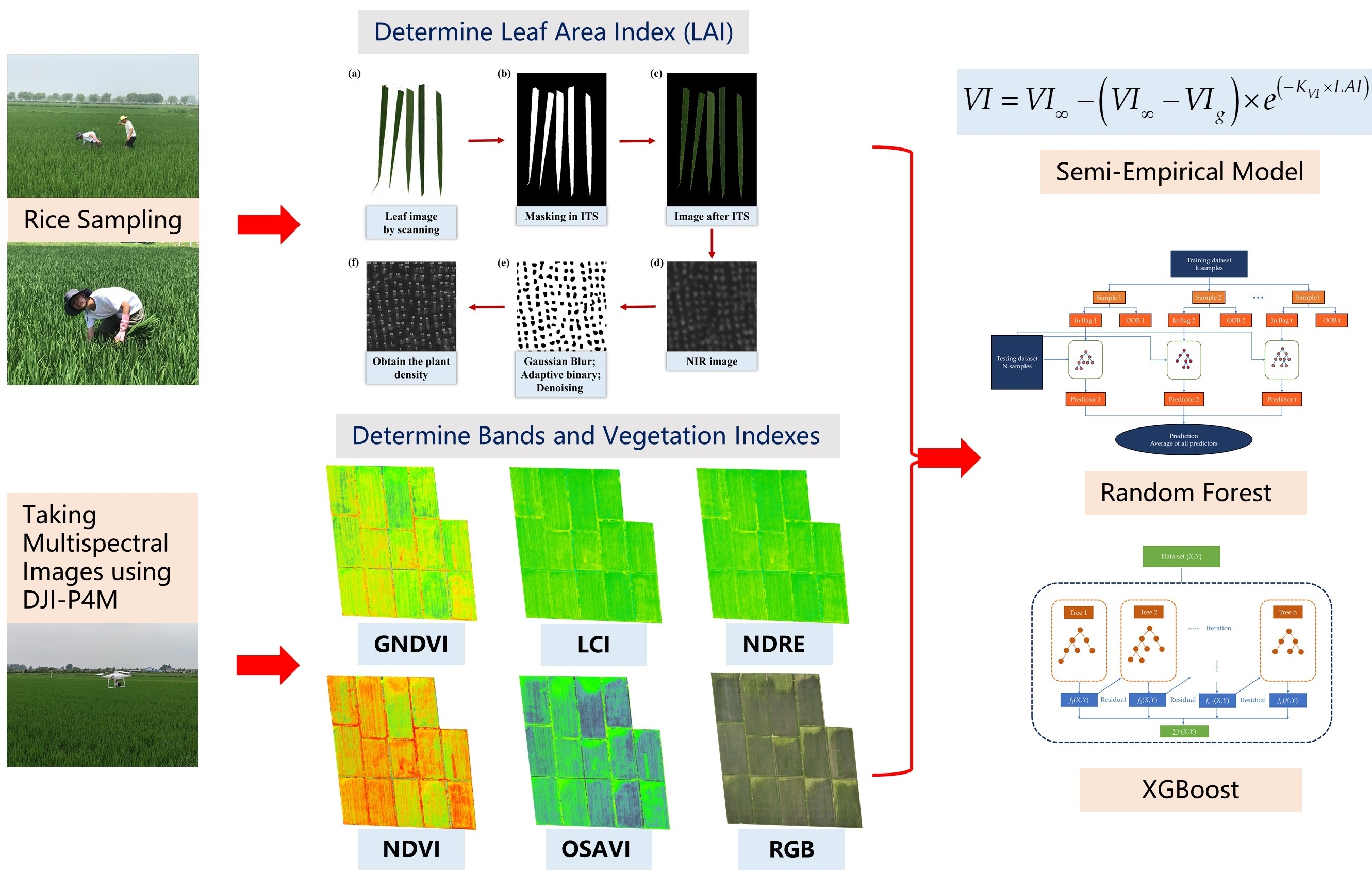
:Accurate estimation of the leaf area index (LAI) is essential for crop growth simulations and agricultural management. This study conducted a field experiment with rice and measured the LAI in different rice growth periods. The multispectral bands (B) including red edge (RE, 730 nm ± 16 nm), near-infrared (NIR, 840 nm ± 26 nm), green (560 nm ± 16 nm), red (650 nm ± 16 nm), blue (450 nm ± 16 nm), and visible light (RGB) were also obtained by an unmanned aerial vehicle (UAV) with multispectral sensors (DJI-P4M, SZ DJI Technology Co., Ltd.). Based on the bands, five vegetation indexes (VI) including Green Normalized Difference Vegetation Index (GNDVI), Leaf Chlorophyll Index (LCI), Normalized Difference Red Edge Index (NDRE), Normalized Difference Vegetation Index (NDVI), and Optimization Soil-Adjusted Vegetation Index (OSAVI) were calculated. The semi-empirical model (SEM), the random forest model (RF), and the Extreme Gradient Boosting model (XGBoost) were used to estimate rice LAI based on multispectral bands, VIs, and their combinations, respectively. The results indicated that the GNDVI had the highest accuracy in the SEM (R2 = 0.78, RMSE = 0.77). For the single band, NIR had the highest accuracy in both RF (R2 = 0.73, RMSE = 0.98) and XGBoost (R2 = 0.77, RMSE = 0.88). Band combination of NIR + red improved the estimation accuracy in both RF (R2 = 0.87, RMSE = 0.65) and XGBoost (R2 = 0.88, RMSE = 0.63). NDRE and LCI were the first two single VIs for LAI estimation using both RF and XGBoost. However, putting more than one VI together could only increase the LAI estimation accuracy slightly. Meanwhile, the bands + VIs combinations could improve the accuracy in both RF and XGBoost. Our study recommended estimating rice LAI by a combination of red + NIR + OSAVI + NDVI + GNDVI + LCI + NDRE (2B + 5V) with XGBoost to obtain high accuracy and overcome the potential over-fitting issue (R2 = 0.91, RMSE = 0.54).

1. Introduction
Leaf area index (LAI) was first introduced by Watson [1] and defined as the sum of the leaf area per unit ground area. LAI is commonly used as an important structural and biophysical indicator of vegetation for crop photosynthesis [2], productivity [3], and water utilization [4]. Moreover, LAI is often required as an input parameter in many models for crop growth diagnosis, biomass estimation, and yield prediction in the application of precision agriculture [5,6,7]. The observations of LAI include direct and indirect measurement methods. The direct measurement of LAI refers to destructive sampling and taking it into the laboratory for measuring. The direct measurement of LAI is generally accompanied by various time-consuming and labor-intensive methods with potential personal errors [8]. Moreover, it cannot provide continuous measurements. Therefore, many research studies focused on the indirect measurement methods for the LAI estimation, and remote sensing technology has been widely used because it has the advantages of non-destructive and quick monitoring [9,10]. For example, Bsaibes, et al. [11] estimated the LAI from the FORMOSAT-2 data, which is so-called “high spatial resolution” and collects images with an 8 m nadir spatial resolution over a 24 km swath. Qu, et al. [12] retrieved high-resolution LAI (15 m) by fusing MOD15 products (1 km resolution), field measurements, and the ASTER reflectance (15 m resolution). Jafari and Keshavarz [13] inversed the LAI from the LANDSAT8 (30 m resolution) and assimilated it with the CERES-Wheat model. However, although the images of satellites have shown great capabilities to estimate the crop LAI at regional to global scales, the relatively sparse spatial resolution (~8 m–1 km) still limits the application of satellites at field scale and in precision agricultural management. Moreover, unfavorable weather conditions, such as clouds or fog, may also reduce the quality of satellite images. As low altitude UAVs are usually simple to operate and have a higher spatial resolution than satellites, and the airborne sensors are also being developed rapidly, more and more studies have applied the UAVs in crop growth monitoring [14,15,16]. For example, Tao et al. [17] estimated and mapped the distribution of LAI for various growth stages of winter wheat using UAV-based hyperspectral data. The hyperspectral sensor in Tao et al. [17] could acquire 125 spectral bands from the visible to the near-infrared wavelengths (450–950 nm). However, the hyperspectral sensors are usually too expensive, which also limits its application in practice. Therefore, much attention has been paid to the low-cost consumer-grade UAV systems consisting of the multispectral sensors or only RGB digital cameras. Barbosa et al. [18] calculated nine RGB (red (R), green (G), blue (B)) vegetation indices (VIs) to estimate the LAI of coffee using the UAV coupled with an RGB digital camera. However, the correlation between RGB VIs and LAI was weak (<0.41). Apolo-Apolo et al. [19] applied a mixed data-based deep neural network (DNN) to estimate the LAI of wheat with RGB images and obtained a high determination coefficient (R2 = 0.81). However, the DNN training needs a huge number of images with different shooting angles. Furthermore, this method only validates in the early stages of crops without the leaves’ shelter and overlap [19]. Meanwhile, a great deal of professional software such as Can-Eye [20] and ImageJ [21] was used for the image pre-processing, which was not easy for local farmers and agricultural managers. Referring to the UAV systems with multispectral sensors, which have advantages and disadvantages between hyperspectral and RGB sensors, usually, the multispectral bands can be used to calculate VIs, and the VIs application can be used to estimate the LAI. For example, Yao et al. [22] proposed a modified triangular VI and obtained high accuracy for wheat LAI estimation (R2 = 0.79) with a narrowband multispectral image. Qi et al. [23] used eight VIs to estimate the peanut LAI from UAV multispectral images. Based on the previous related studies, the VI is an important factor affecting the LAI estimation accuracy, and the most common VIs include the Ratio Vegetation Index (RVI) and the Normalized Difference Vegetation Index (NDVI) [24]. Moreover, the VIs were also improved to minimize the interference of other factors such as soil and atmospheric disturbance, including the Soil-Adjust Vegetation Index (SAVI) [25], the optimized SAVI (OSAVI) [26], the improved SAVI [27], the Atmospheric-Resistant Vegetation Index (ARVI) [28], the Enhanced Vegetation Index (EVI) [29], and the Wide Dynamic Range Vegetation Index (WDRVI) [30]. Besides the VI detection in the fields, multispectral sensors with UAV also have other applications in the view of ecological aspects [31,32]. For example, Lama et al. [33] used the UAV-based NDVI to assess the impact of riparian vegetation morphometry on bulk drag coefficients distribution along an abandoned vegetated drainage channel. In addition, a large number of studies confirmed that the near-infrared (NIR) band has better inversion ability of vegetation canopy [24,25,26,27,28,29,30]. Different from the visible light camera, which has only three bands of red, green, and blue, the use of a multispectral camera with an NIR band has more advantages than the visible light image. Therefore, our study selected the multispectral images for estimating the LAI. Nevertheless, the calculation of VIs also needs several pre-treatment steps for the multispectral images, calling for professional skills and domain specific expertise.
Another factor affecting the LAI estimation accuracy is the algorithm. Besides the process-based method such as the radiative transfer model, which is not the focus of this study, the VI-based algorithms are usually empirical or semi-empirical. Peng et al. [34] estimated the LAI from VIs by four empirical models including the linear model, the exponential model, the logarithmic model, and the quadratic polynomial model. Dong et al. [35] estimated the LAI of spring wheat and canola using eight VIs by a semi-empirical model based on the modified Beer’s law. In the later stages of crop growth, the VIs move closer to saturation because the field is almost covered with plant leaves. Moreover, due to the dynamic change of LAI, there would be multiple collinearities between different VIs and the LAI. Therefore, the machine learning models are increasingly applied for LAI estimation. Reisi Gahrouei et al. [36] applied an artificial neural network (ANN) and support vectors regression (SVR) to estimate the LAIs of canola, corn, and soybeans with the VIs from the multispectral images and indicated that SVR provided better accuracy than ANN. Maimaitijiang et al. [37] predicted the soybean’s LAI with the VIs by four machine learning models including partial least squares regression (PLSR), random forest (RF), SVR, and extreme learning regression (ELR). However, a classical shortcoming of the machine learning models is over-fitting. Recently, the Extreme Gradient Boosting (XGBoost) algorithm proposed by Chen and Guestrin [38] based on GBDT and RF models was proven as a novel implementation method for gradient boosting machines (GBMs) and classification and regression trees (CART) with the ability to reduce over-fitting [39,40,41]. However, the accuracy of XGBoost for estimating LAI was not evaluated. Moreover, previous studies mainly used only one of the VIs or selected some of the VIs as input variables for the empirical models, while very few studies explored the effects of different combinations of VIs on the LAI estimation. In addition, the conversion from spectral bands to VIs may lose some information, while almost no study evaluated the effects of combinations of spectral bands and VIs together on the LAI estimation.
Therefore, this study conducted field experiments in Yancheng, Jiangsu Province, China and used the DJI Phantom 4 Multispectral (DJI-P4M, SZ DJI Technology Co., Ltd., Shenzhen, China) UAV to obtain both multispectral and RGB images of rice and establish the observation dataset. The observation dataset included five bands and five VIs retrieved from the UAV images and the observed LAI from the field experiments. The objectives of this study were to (1) establish the rice LAI estimation model by XGBoost and compare the accuracy with RF and semi-empirical (SEM) models, (2) evaluate the effects of different combinations of spectral bands and VIs on the rice LAI estimation accuracy, and (3) find out the optimal combinations of both spectral bands and VIs for rice LAI estimation for different models.
2. Materials and Methods
2.1. Study Site
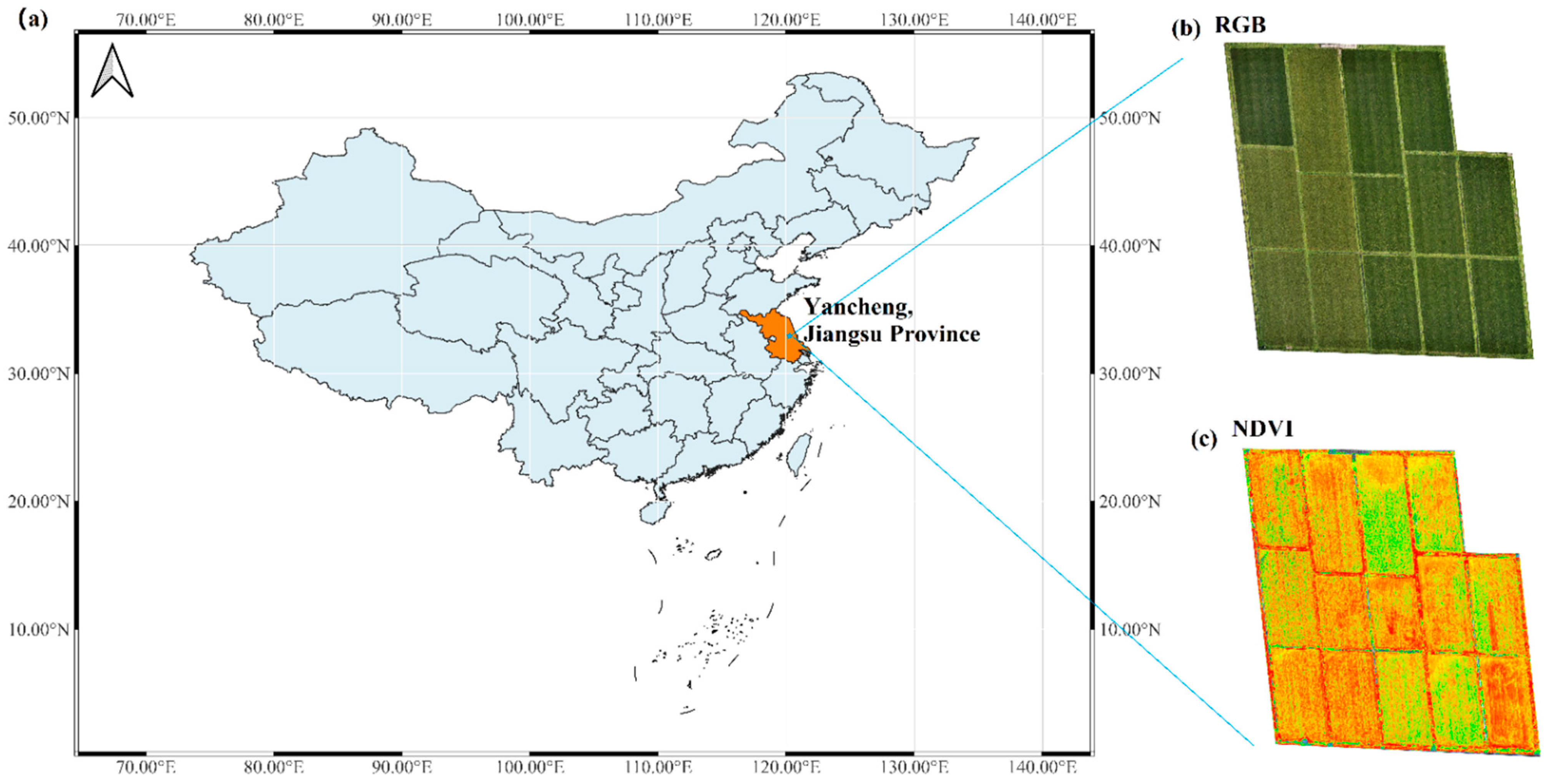
The field experiments were carried out in 14 fields of the Qixing farm (33°11′01’’N, 119°52′53.8’’E), Yancheng, Jiangsu Province, China from April to October 2020 (Figure 1). Yancheng is located between the northern subtropical zone and the southern warm temperate zone. The average annual precipitation is around 1014.7 mm, and the average annual runoff is about 3.96 billion m3. All 14 fields were irrigated with water pumps and pipes and connected to the drainage ditches, while the outlet of the main ditch was a river.
The soil texture of top 0–60 cm depth of the fields was clay loam. pH, organic matter (OM), alkali hydrolysable nitrogen content, effective phosphorus content, effective potassium content, and effective zinc content were 7.4, 24.4 g·kg−1, 180.2 mg·kg−1, 24.2 mg·kg−1, 242.8 mg·kg−1, 0.7 mg·kg−1 respectively. Three varieties of rice including glutinous rice, indica rice, and japonica rice were planted in the experiments. The seedling and the transpla4nting dates of all three varieties were 21 April 2020 and 30 May 2020, respectively. The harvest date of indica rice was 14 September 2020, and the harvest date of glutinous rice and japonica rice was 23 October 2020.
2.2. Data Collection
2.2.1. Multispectral Images
Multispectral images were captured by an unmanned aerial vehicle (UAV) of DJI Phantom 4 Multispectral (DJI-P4M, SZ DJI Technology Co., Ltd., Shenzhen, China) 10 times for indica rice (12 June, 21 June, 26 June, 1 July, 6 July, 13 July, 20 July, 2 August, 14 August, and 25 August in 2020) and 12 times for glutinous rice and japonica rice during the crop growing season (12 June, 21 June, 26 June, 1 July, 6 July, 13 July, 20 July, 2 August, 14 August, 25 August, 17 September, and 23 October in 2020).
Six cameras were installed in the DJI-P4M, which contained the bands of red edge (RE, 730 nm ± 16 nm), near-infrared (NIR, 840 nm ± 26 nm), green (560 nm ± 16 nm), red (650 nm ± 16 nm), blue (450 nm ± 16 nm), and visible light (RGB). Based on the bands except for RGB, five vegetation indexes (VI) including Green Normalized Difference Vegetation Index (GNDVI), Leaf Chlorophyll Index (LCI), Normalized Difference Red Edge Index (NDRE), Normalized Difference Vegetation Index (NDVI), and Optimization Soil-Adjusted Vegetation Index (OSAVI) were calculated from the bands (Equations (1)–(5)).
2.2.2. Plant Sampling and Leaf Area Index
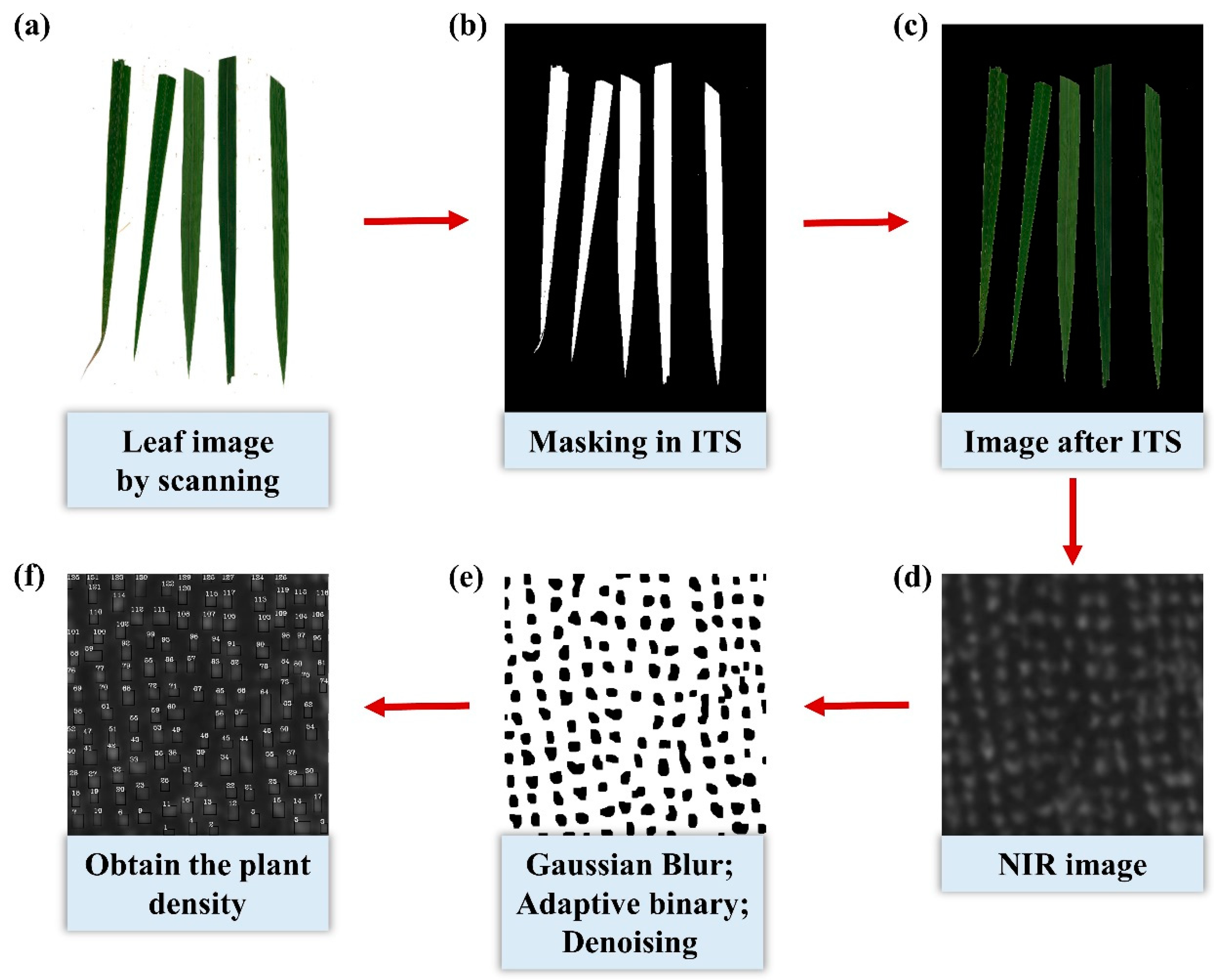
During the crop growth period, rice plants in 14 fields were sampled 8 times on the same day of the UAV data collection (June 12, June 21, July 1, July 13, July 20, August 2, August 14, and August 25 in 2020). Three samples were selected and cut from the junction between the root and the stem, and the leaves were separated from the plants using scissors for each field. In each sampling, 42 plants (3 plants × 14 field) were taken in 14 fields. Therefore, 336 plants were taken during the whole experiments. However, due to the operation miss, 324 plants in total were used in our study. The leaves were then scanned with a resolution of 300 PPI (EPSON V39 Scanner), and the leaf area was determined by image threshold segmentation (ITS) and specific leaf area (SLA, cm2·g−1).
In the ITS, the images were first converted to the HSV (hue, saturation, value) color space using the OpenCV library of Python [42]. After that, the leaf threshold was manually segmented (Figure 2a–c), and the leaf areas (LA, cm2) were calculated from the number of leaf pixels (NLP) (Equation (6)).
After scanning, the leaves were put at 105 °C for 30 min, then dried at 75 °C to a constant weight, and the dry matter of the leaves (DML, g) was weighed. The SLA was calculated by Equation (7), and the LA of a single plant (LAS, cm2·plant−1) was calculated by SLA and the dry matter of leaves of the single plant (DMLS, g) (Equation (8)).
The plant density (PD, plant·cm−2) of each field was determined from the NIR band image captured by DJI-P4M using the OpenCV library of Python (Figure 2d–f). More exactly, the NIR images were treated by several steps including Gaussian blur [43], adaptive binary [44], and denoising with closing operation of the convolution kernel [45]. After that, the LAI was calculated using LAS and PD (Equation (9)).
In total, 324 pairs of observation data were collected with the observed LAI and five VIs.
2.3. Semi-Empirical Model (SEM)
An SEM in the form of the modified Beer’s law was used to calculate the LAI of rice (Equation (10)) [46,47].
In Equation (10), the VI∞ is the VI value for the infinitely dense green canopy; KVI is the extinction coefficient linking LAI and the VI; VIg is the VI value of bare soil. To calculate the LAI, three parameters of the SEM (KVI, VI∞, and VIg) needed to be determined and were estimated from the observations using the Metropolis–Hastings Markov chain Monte Carlo (MCMC) algorithm [48]. More exactly, five VIs including GNDVI, LCI, NDRE, NDVI, and OSAVI were used as VIs in Equation (10) to fit KVI, VI∞, and VIg with the observed LAI one by one. To enhance the credibility and the reliability, the 324 pairs of data were divided into the training and the test datasets. There were 240 and 84 pairs of data in the training and the test datasets, respectively.
2.4. Random Forest Model (RF)
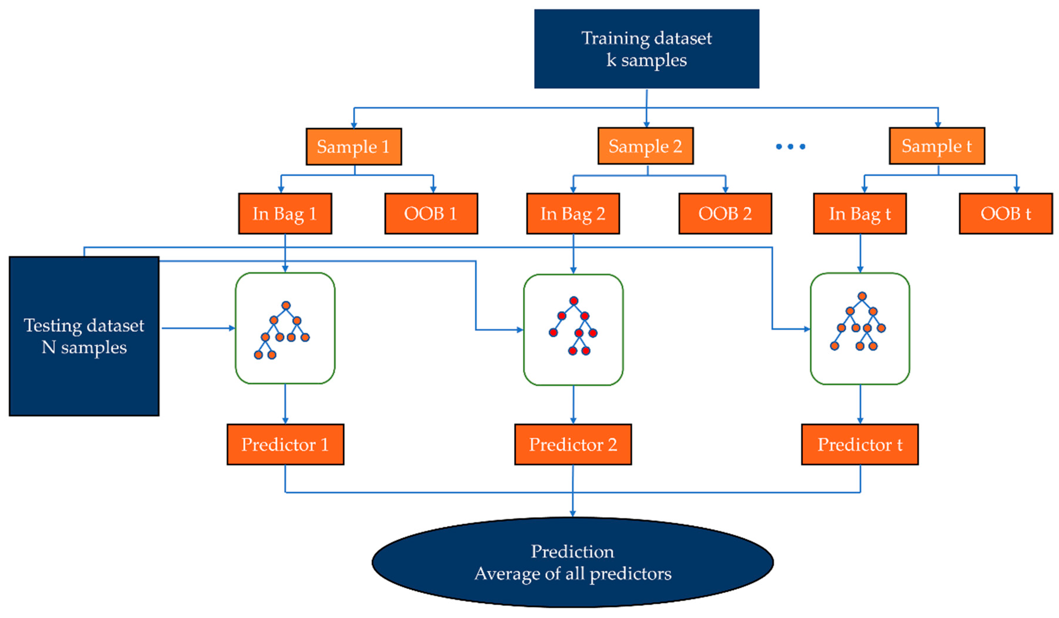
The RF was developed by Breiman [49] based on CARTs and bagging (bag) methods (Figure 3). RF is an ensemble classifier composed of a series of decision trees. Each tree in the forest makes independent predictions based on the characteristics of its own test data and finally uses a voting method (the minority obeys the majority) to make the final prediction. More exactly, the RF selects k sub-training sample sets from the total data set D to form k decision trees (D1, D2, …, Dt, …, Dk), Based on Dt, a basic decision tree model can be formed. After that, the test data are inputted into each decision tree of RF, and the risk level corresponding to each leaf node is the evaluation result of the decision tree. In addition, the RF method uses bootstrapping to perform random sampling with replacement to obtain different sample data. The datasets not included in the model are called “out-of-bag” (OOB). Using different sample data to train the decision tree can successfully reduce the correlation of samples. Moreover, the node selection of RF was also random, which further reduced the correlation of samples, basically solving the over-fitting problem of a single decision tree model and causing RF to have a good tolerance to noise. Further details about RF can be found in Breiman [49]. The training and the test samples for RF were 204 and 120 pairs of the data, respectively, which was the same as the XGBoost. The RF was implemented using the package “randomForest” in R software (version 4.0.2), and this package also offered the important feature selection analysis including the indexes of IncMSE and IncNodePurity. More exactly, the IncMSE referred to the increase in the estimated error with a randomly selected variable compared with the original estimated error. The larger the IncMSE value was, the more important the variable was. The IncNodePurity referred to the degree of influence of this variable on each decision tree node. The larger the IncNodePurity value was, the more important the variable was [50].
2.5. Extreme Gradient Boosting Model (XGBoost)
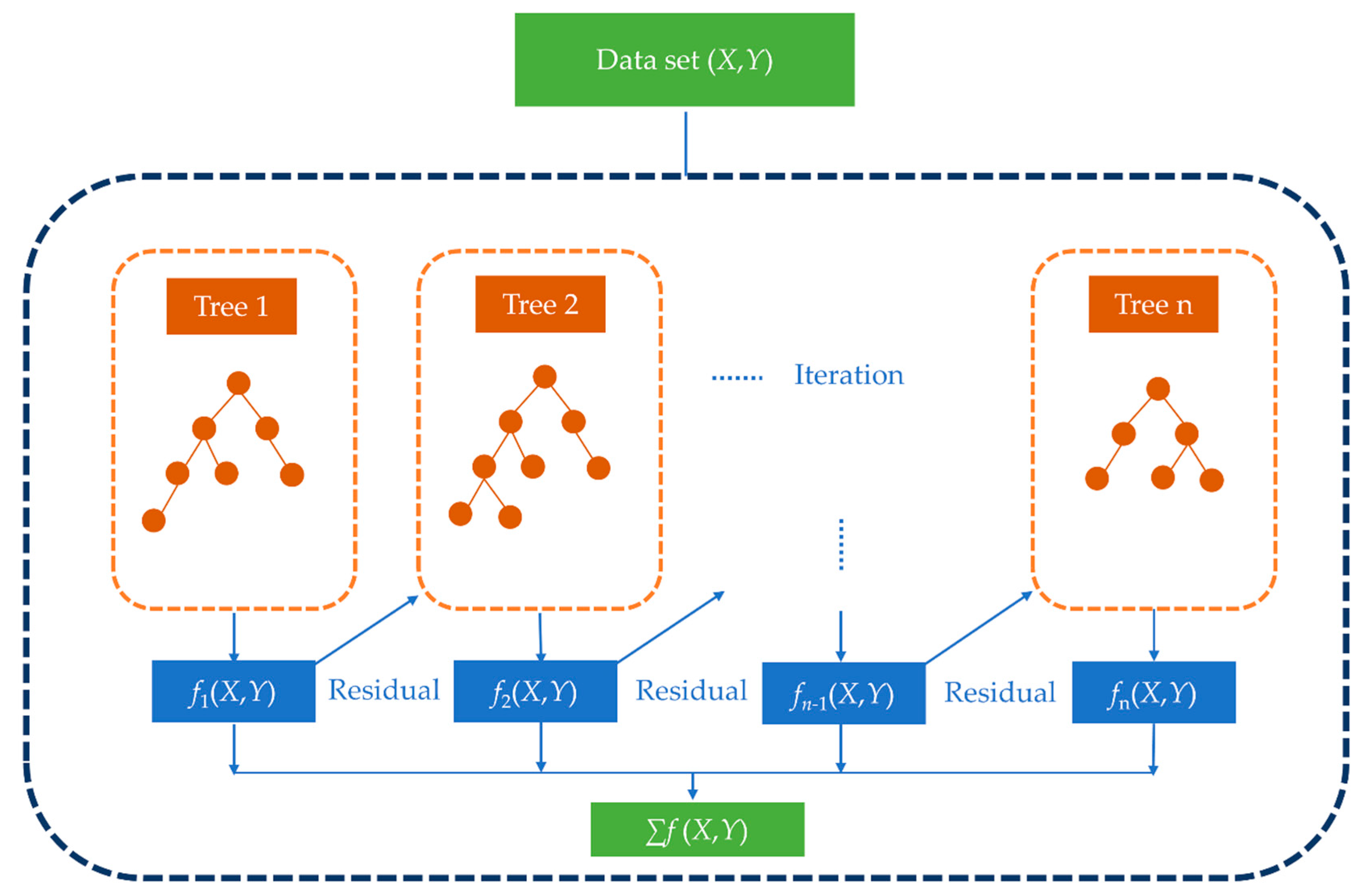
The XGBoost is a new, efficient ensemble learning algorithm established by Chen and Guestrin [38], which is an improved algorithm of gradient boosting and uses the Taylor expansion to obtain the second derivative as an independent variable (Figure 4). The boosting algorithm is based on the concepts of strong and weak learnable problems given by Kearns and Valiant [51], who proposed a very interesting theorem: a problem is strongly learnable if and only if it is weakly learnable. The XGBoost integrates several “weak” learners to generate a “strong” learner by additive learning. The prediction function of XGBoost can be given in Equation (11).
In Equation (11), yi,p is the predicted value, f(xi) is a learner, K is the number of learners, and xi is the input data.
To evaluate the fitting effect, the loss function (ψ) was determined as Equation (12).
In Equation (12), l is the function that indicates the size of the residual between the predicted and the observed values. Ω is the regularization term, which indicates the complexity of the model (Equation (13)).
In Equation (13), γ is the mini loss, T is the label set of the leaf node of the regression tree, λ is the regularization parameter, and ω is the score vector.
More details about XGBoost can be found in Chen and Guestrin [38]. Different from the SEM, there were 204 and 120 pairs of data in the training and the test datasets, respectively.
The XGBoost was implemented using the package “xgboost” in R software (version 4.0.2). Similar to RF, this package also offered the important feature selection analysis including the indexes of gain, cover, and frequency. The gain implies the relative contribution of the corresponding feature to the model calculated by taking each feature’s contribution for each tree in the model. The cover metric means the relative number of observations related to this feature. The frequency is the percentage representing the relative number of times a particular feature occurs in the trees of the model [52].
2.6. Statistical Evaluation
Grid-search method was used for the training of RF and XGBoost. Tuning parameters of RF are “number-of-tree” and “max-feature”. The range of number-of-tree was 50–500, and the interval was 50. The max-feature was set as the square root of the feature. XGBoost model has 3 parameters that needed to be tuned, which are “number-of-tree”, “learning-rate”, and “max-depth-of-tree”. The range of number-of-tree was also 50–500, and the interval was also 50. The range of learning-rate was 0.01–0.3, and the interval was 0.05. The range of max-depth-of-tree was 1–15, and the interval was 3. The tuned parameters of RF and XGBoost with different inputs are indicated in Table S1.
The evaluation statistics used in this study included determination coefficient (R2), normalized root mean squared error (RMSE), mean absolute error (MAE), Nash–Sutcliffe coefficient (NSE), and mean absolute percentage error (MAPE) (Equations (14)–(18)).
In Equations (14)–(18), Oi, Pi, Oave, and Pave are observed LAI, predicted LAI, mean of observed LAI, and mean of predicted LAI, respectively. Higher R2 and NSE values indicate better model performance, and the regression line fits the data well. Conversely, the lower values of RMSE, MAE, and MAPE show better prediction accuracy.
3. Results and Discussion
3.1. Performance of the Semi-Empirical Model (SEM)
The scatterplots between VIs and LAI of the SEM in the test process are shown in Figure 5 with the parameters (KVI and VI∞) in Table 1 (the parameters were fitted in the training process, while the statistical indexes were determined in the test process). Although the VIg was also a parameter in the SEM (Equation (10)), the fitted value of VIg in our study was almost zero for all inputs, which was similar to the study of Dong et al. [35]. Gonsamo [53] also concluded that the contribution of VIg on the final LAI estimation was far less than that of VI∞. With the five VIs as the input, KVI and VI∞ ranged from 0.285 to 0.899 and 0.540 to 0.950, respectively. Using GNDVI as the input obtained the highest accuracy for LAI prediction. More exactly, R2 and NSE were both 0.780, while RMSE, MAE, and MAPE were 0.770, 0.540, and 0.240, respectively. Previous studies also indicated that the GNDVI was more stable than NDVI by replacing the red band with the green band of NDVI and had higher LAI prediction accuracy than NDVI [54,55]. The LCI and the NDVI had similar accuracies for LAI prediction with GNDVI using SEM. The R2s of LCI and NDVI were 0.77 and 0.75, while the RMSEs were 0.80 and 0.82, respectively. The NDRE had the lowest accuracy for LAI prediction, and R2, NSE, RMSE, MAE, and MAPE were 0.67, 0.35, 1.31, 0.90, and 0.40, respectively. The LCI and the NDRE were usually applied in predicting the chlorophyll content. However, Simic Milas et al. [56] also found that NDRE correlated with the LAI of corn (R2 = 0.62), which also had similar accuracy with our study. Moreover, the lower accuracy of NDRE compared with LCI could be because NDRE had a higher relationship with the crop’s chlorophyll content in the late stages compared to the early stages [57,58]. Moreover, the biases between predicted LAI and the 1:1 line (dash lines in Figure 5) for all VIs as inputs were larger when the LAI > 2. The reason might be the VIs became insensitive to the LAI as light absorption by chlorophyll became saturated at high LAI [59].
3.2. Machine Learning Models with Multispectral Band
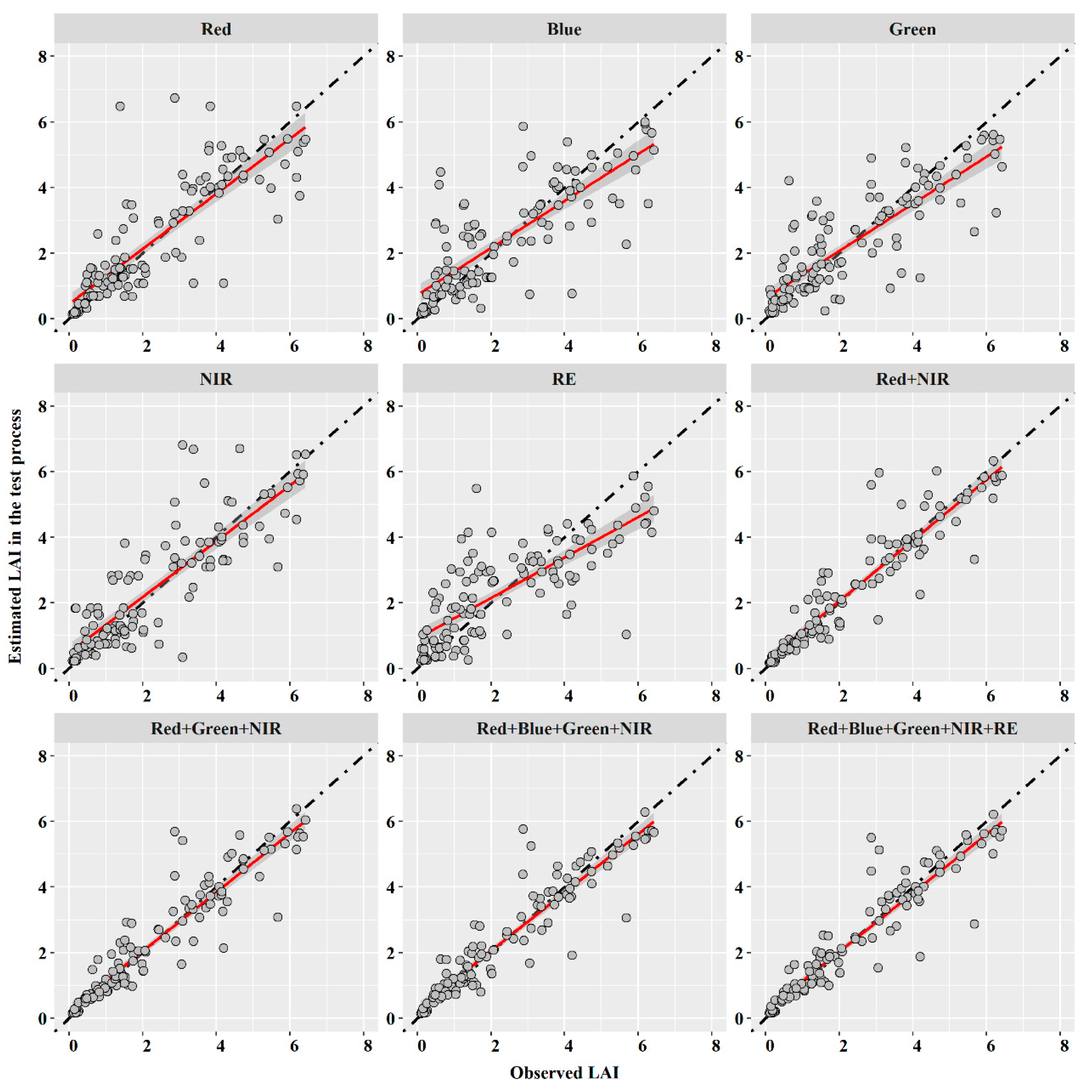
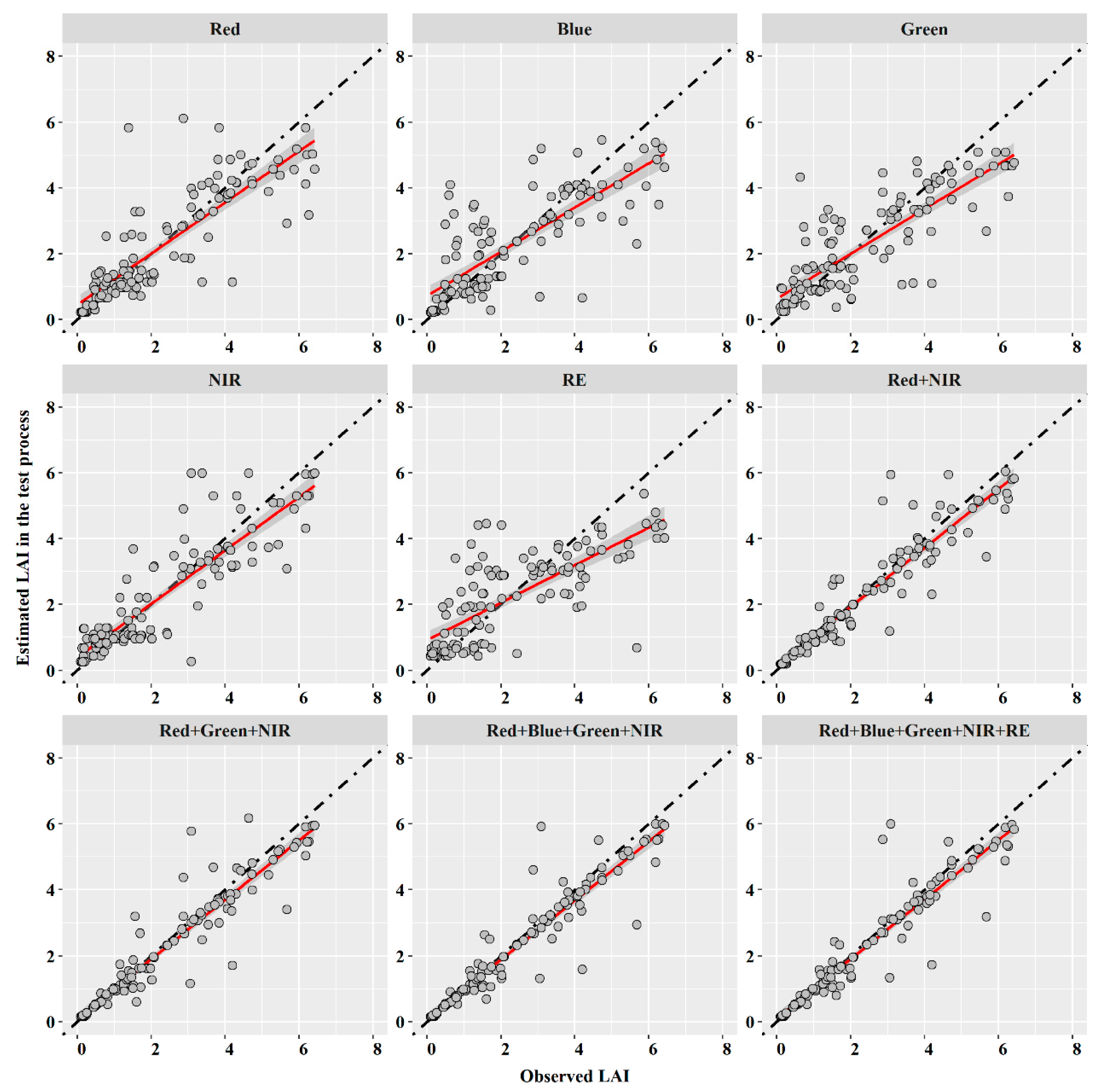
For RF, the order of prediction accuracy (test process) of LAI for the five bands was NIR > red > green > blue > RE (Figure 6). The R2 and the RMSE of the five bands were 0.733, 0.706, 0.688, 0.629, and 0.596 and 0.988, 1.039, 1.025, 1.136, and 1.167, respectively (Table 2). NIR and red are popular bands used to calculate VIs such as Difference Vegetation Index (DVI) [60] and OSAVI [26]. Considering NIR and red were the first two accurate input variables, the combinations of NIR and red were treated as the input variables of RF together. The NIR and the red combination had higher prediction accuracy than the single NIR or red as an input variable. More exactly, R2 and NSE of the NIR and red combination were 0.875 and 0.872, increasing 19.4% and 23.0% compared with single NIR as an input variable, respectively. Furthermore, RMSE, MAE, and MAPE of the NIR and red combination were 0.655, 0.392, and 0.171, only accounting for 66.3%, 57.1%, and 57.2% of the single NIR as an input variable, respectively. However, adding more bands into the combination could only increase the accuracy slightly. For example, the highest accurate combination of bands was red, blue, green, NIR, and RE. The R2 and the NSE of this combination were 0.889, only increasing 1.60% and 1.95%, respectively, compared with the combination of NIR and red. Meanwhile, RMSE, MAE, and MAPE of the combination of five bands were 0.612, 0.369, and 0.161, respectively, only decreasing by 6.56%, 5.86%, and 5.85% compared with the combination of NIR and red.
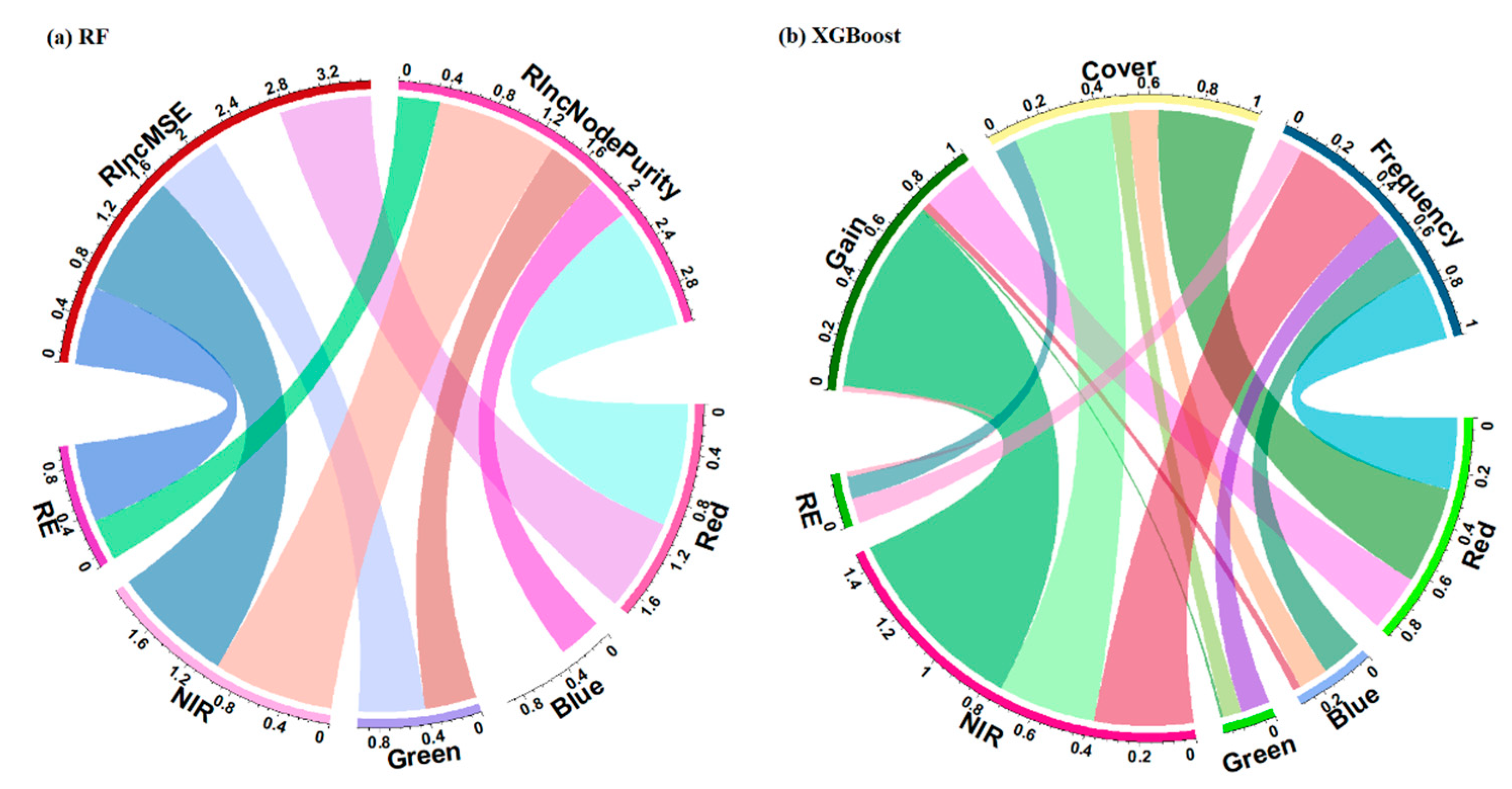
This phenomenon can be explained by the important feature selection analysis [50,61]. More exactly, the order of increase in mean square error (IncMSE) and increase in node purity (IncNodePurity) of the five bands is indicated in Figure 7a. To make the IncMSE and the IncNodePurity comparable, all values were converted into the relative value (ranged from zero to one) by dividing the maximum IncMSE or IncNodePurity, respectively. Figure 7 indicates that the NIR had the maximum relative IncMSE (RIncMSE, 1.00) and secondary relative IncNodePurity (RIncNodePurity, 0.99), while the red had the secondary RIncMSE (0.75) and the maximum RIncNodePurity (1.00).
Similar to RF, the order of prediction accuracy (test process) of LAI for the five bands using XGBoost was also NIR > red > green > blue > RE (Figure 8). The R2 and the RMSE of the five bands were 0.771, 0.720, 0.698, 0.630, and 0.574 and 0.881, 0.980, 1.012, 1.119, and 1.197, respectively (Table 2). The chord also showed that the three importance indicators (gain, cover, and frequency) of NIR and red were all larger than other bands (Figure 7b) [52]. More exactly, the values of gain, cover, and frequency of NIR and red were 0.726, 0.368, and 0.375, and 0.214, 0.366, and 0.268, respectively. Moreover, the accuracy of XGBoost was higher than RF when only one band was the input variable. For example, using NIR as the input variable obtained R2 and NSE of 0.771 and 0.769 of XGBoost, increasing 5.18% and 8.46% compared with the RF. Similar results were also found in solar radiation and reference evapotranspiration prediction [62]. Furthermore, using NIR and red bands as input variables also increased the prediction accuracy in the XGBoost. Specifically, R2 and NSE of the NIR and red combination were 0.883 and 0.879, increasing 14.5% and 14.3% compared with single NIR as an input variable, respectively. Furthermore, RMSE, MAE, and MAPE of the NIR and red combination were 0.636, 0.377, and 0.164, only accounting for 72.2%, 59.3%, and 59.2% of the single NIR as an input variable, respectively. This is consistent with previous studies which found that NIR and red bands can better reflect vegetation conditions [25,63]. However, different from the RF, the highest accurate combination of bands was red, blue, green, and NIR; adding RE into the combination decreased the prediction accuracy slightly. This indicates that RE does not contribute much to LAI prediction and causes slight over-fitting of the model [64]. In addition, adding more bands into the combination could only increase the accuracy slightly, which was also similar to the RF. For example, the highest R2 and NSE in the XGBoost were 0.900 and 0.894, respectively, only increasing 1.93% and 1.71% compared with using the NIR and red combination as the input variable. However, the accuracy of XGBoost was only slightly higher than RF with combined bands as input variables. The highest R2 and NSE of XGBoost increased only 1.24% and 0.56%, while RMSE, MAE, and MAPE of XGBoost decreased only 2.61%, 14.36%, and 14.29%, respectively, compared with the RF.
3.3. Machine Learning Models with Vegetation Index
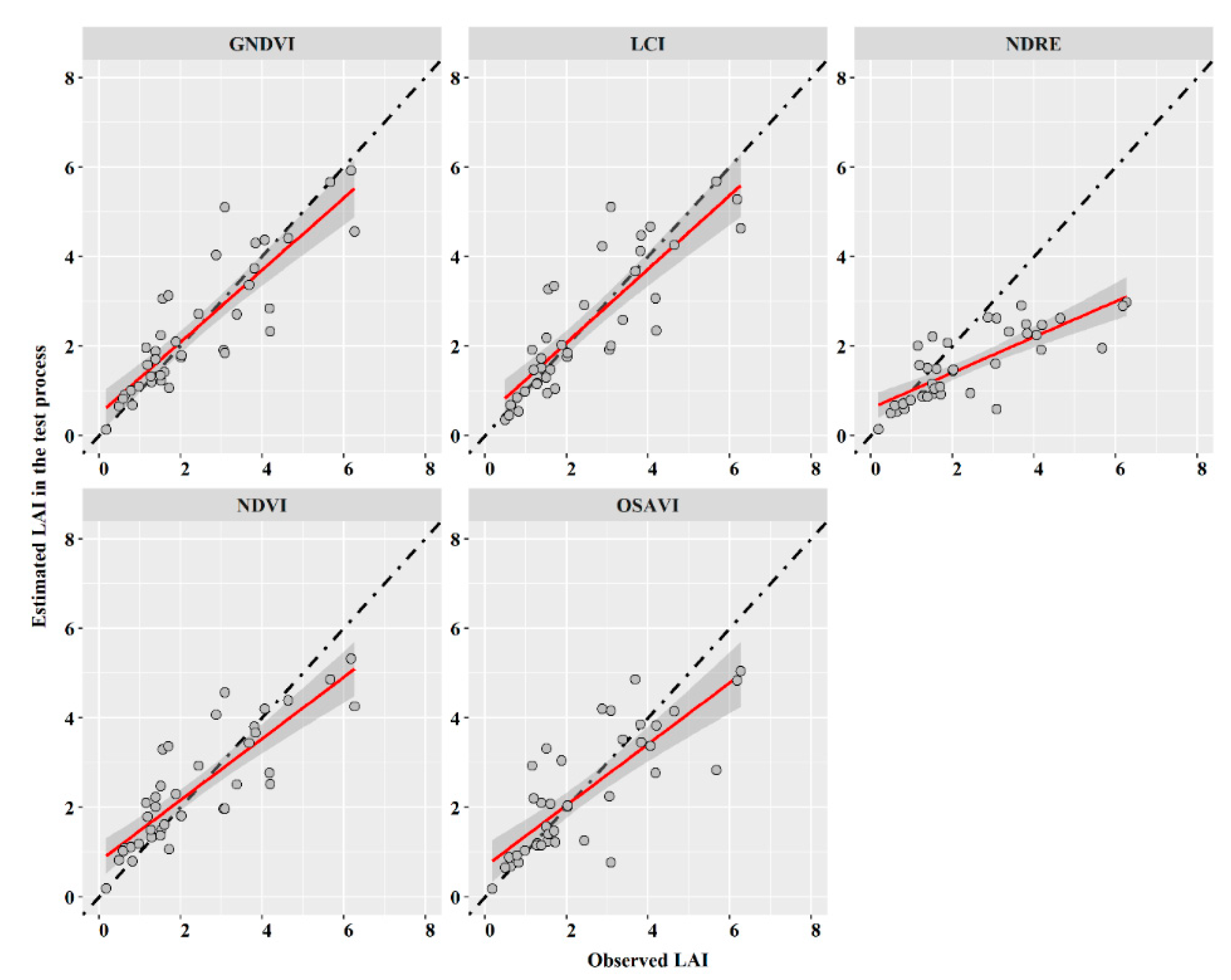
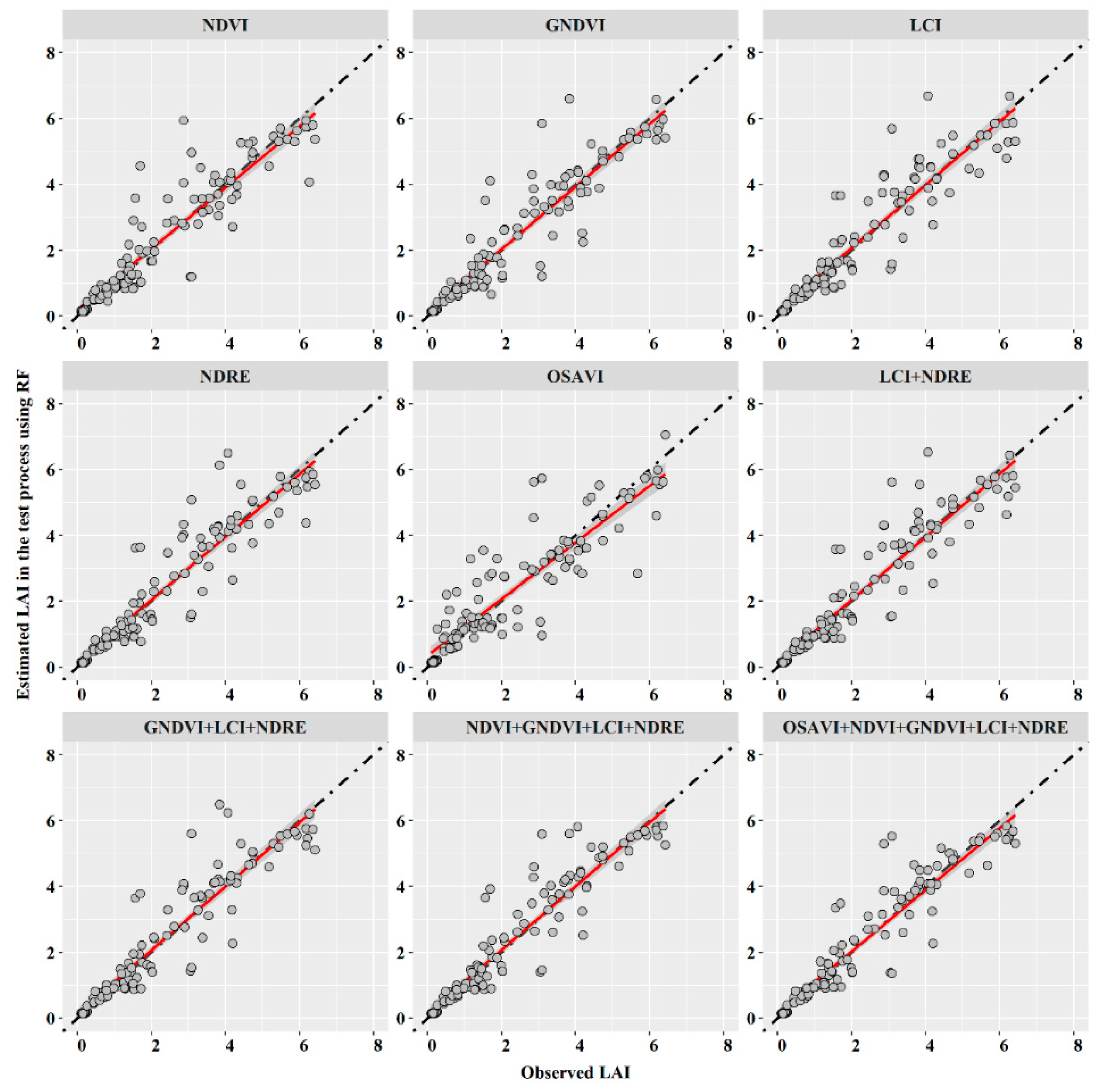
For RF, prediction accuracy (test process) of LAI for the four VIs except OSAVI was very close, and the first two accurate VIs were NDRE and LCI (Figure 9). The ranges of R2, NSE, RMSE, MAE, and MAPE of the four VIs except OSAVI were 0.861–0.875, 0.856–0.867, 0.667–0.696, 0.409–0.420, and 0.178–0.183, respectively (Table 3). The lowest accurate VI was OSAVI. Although OSAVI only decreased the R2 (0.811) by 7.31%, it increased 20.54% of RMSE compared with NDRE. The reason might be the OSAVI considering the effect of soil on the crop’s chlorophyll content, which could improve the LAI prediction in the early growth stages [26,65]. However, the effect of soil on rice’s LAI could be almost ignored, as the soil surface was covered with about 4 cm water depth (observed in the experiment). Meanwhile, putting more than one VI together as a combination could not improve the prediction accuracy. For example, the highest accuracy was the combination with all five VIs as the input variables, which had R2 and NSE of 0.892 and 0.890, increasing by only 1.94% and 2.65% compared with using NDRE as the single input variable. The importance analysis also showed similar results: RIncMSE and RIncNodePurity of the five VIs were very close except the OSAVI (Figure 10a).
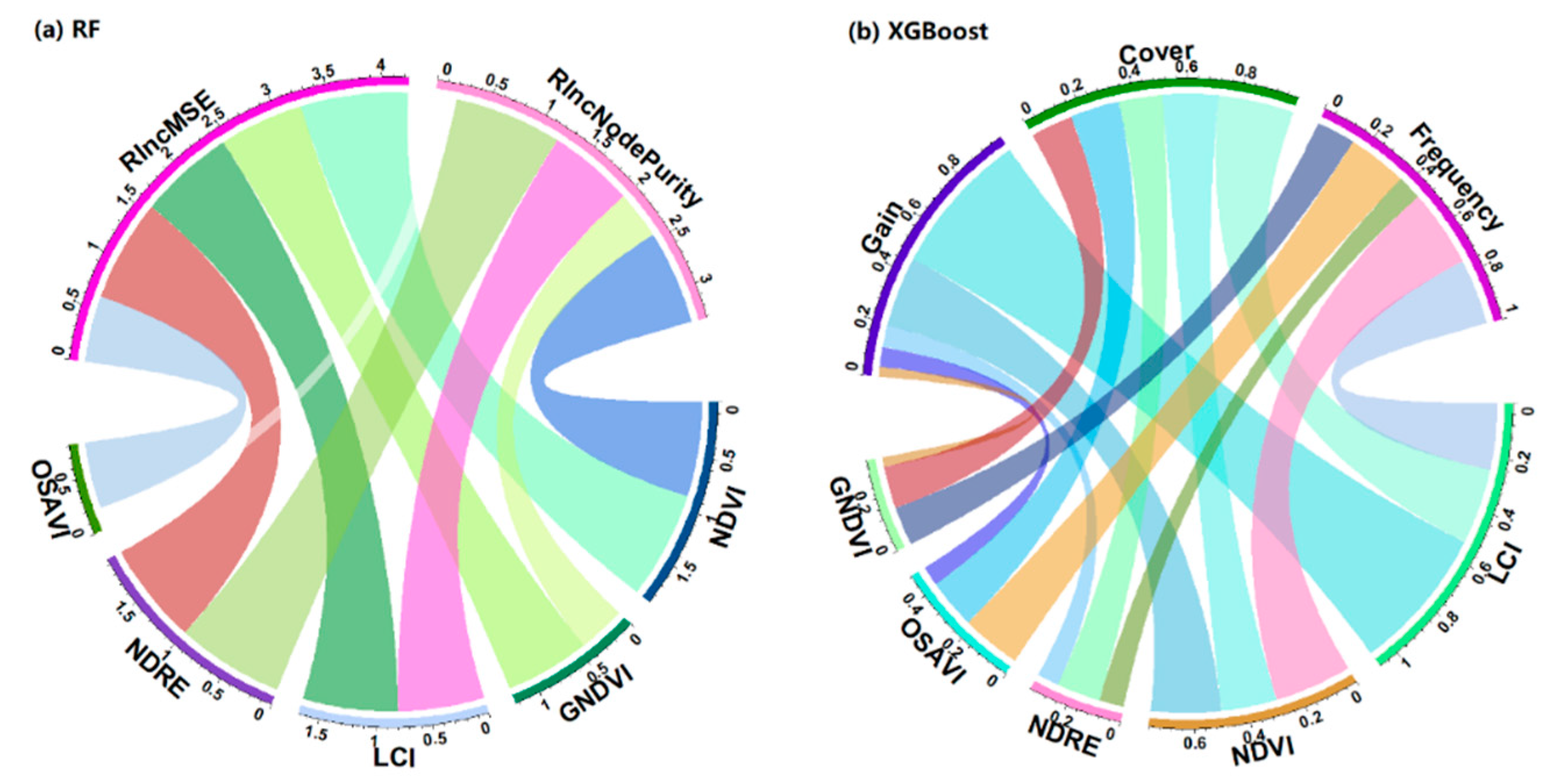
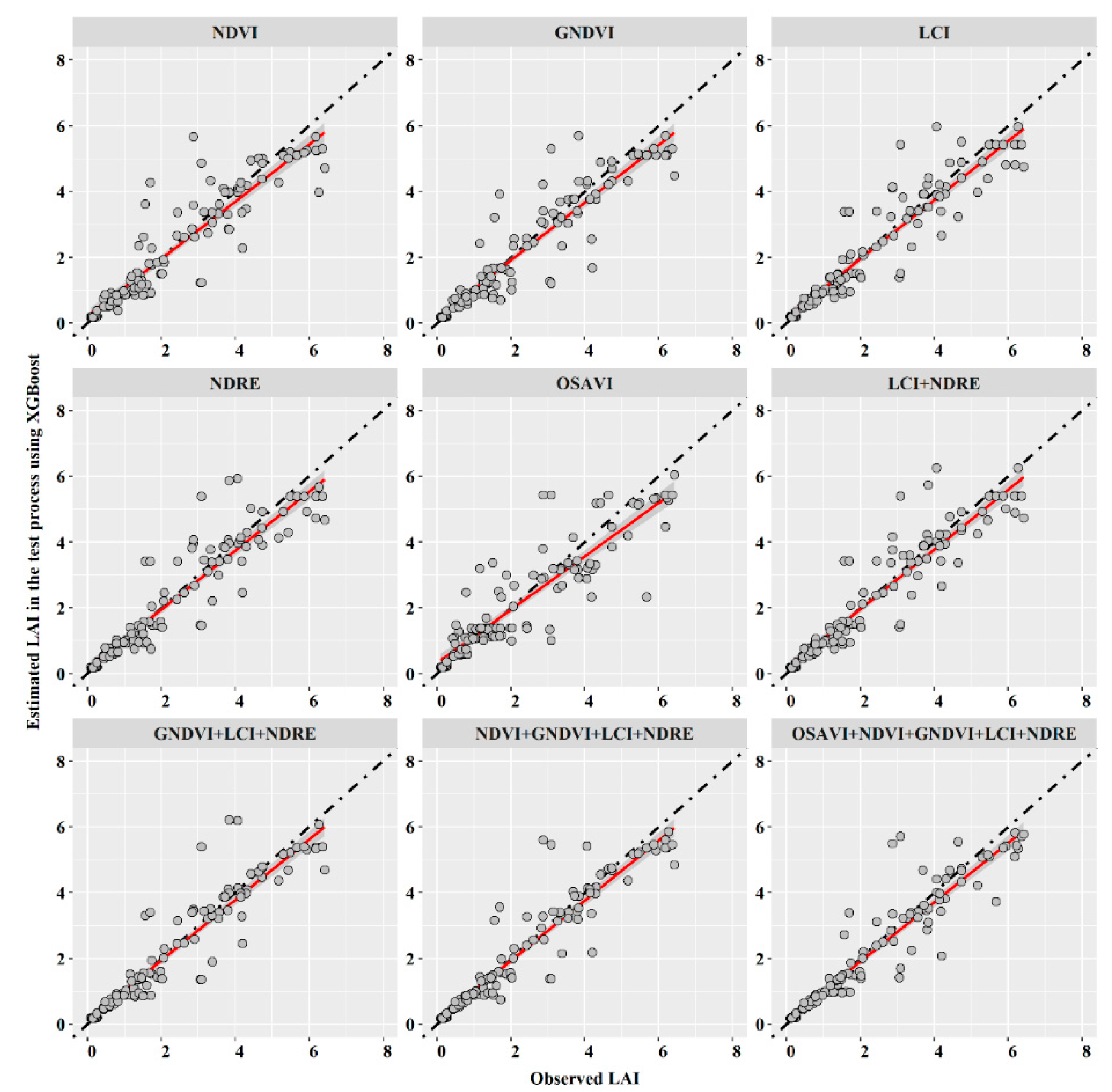
For XGBoost, using LCI as the input variable had slightly higher accuracy than NDRE, which was different from RF (Figure 11). The R2 and the RMSE with LCI were 0.881 and 0.879, respectively, which increased 1.03% and 1.15% compared with NDRE. Moreover, prediction accuracy (test process) of LAI for the four VIs except OSAVI was also very close, which was similar to the RF. The ranges of R2, NSE, RMSE, MAE, and MAPE of the four VIs except OSAVI were 0.883–0.881, 0.851–0.879, 0.637–0.708, 0.397–0.431, and 0.173–0.188, respectively (Table 3). The lowest accurate VI was also OSAVI, which decreased 7.71% and 7.96% of R2 and NSE, while it increased 25.59%, 34.00%, and 34.10%, respectively, compared with using LCI as the single input variable. However, putting more than one VI together as a combination could not improve the prediction accuracy obviously, which was similar to RF. For example, the most accurate combination of VIs was NDVI, GNDVI, LCI, and NDRE in XGBoost; R2 and NSE of this combination were 0.890 and 0.886, respectively, only increasing 1.02% and 0.80% compared with using LCI as the single input variable. Meanwhile, RMSE, MAE, and MAPE of the above combination were 0.617, 0.341, and 0.148, which decreased 3.14%, 14.1%, and 14.5% compared with using LCI as the single input variable, respectively. Figure 10b also indicates that the LCI was the most important VI for the LAI estimation compared with other VIs. For example, the gain value of LCI was 0.544, which increased 106% compared to the NDVI. Moreover, the gain value of other three VIs (NDRE, OSAVI, GNDVI) could be ignored compared with LCI. Meanwhile, four VIs (except OSAVI) also obtained the highest accuracy in XGBoost, while all five VIs were needed for the highest prediction accuracy of LAI by RF, which was also in accordance with using the bands as input variables.
In addition, the order of importance indicators in both RF and XGBoost for the VIs was not strictly the same with the LAI estimation accuracy of a single VI, which was different from the bands as input variables. The possible reason was the VIs were the non-linear arithmetic combination of bands.
3.4. Machine Learning Models with Multispectral Band and Vegetation Index
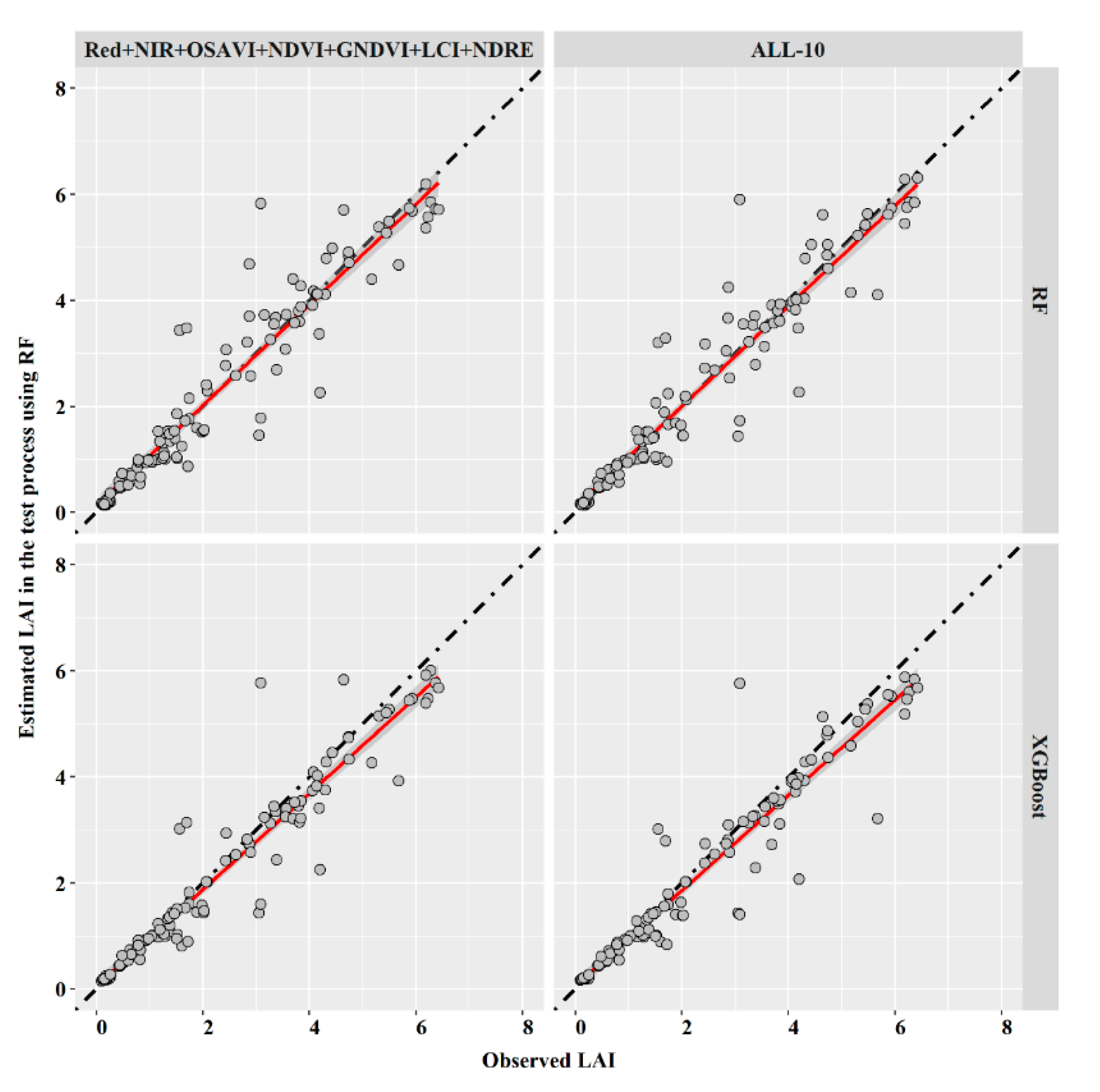
The above analysis indicated that both RF and XGBoost improved the prediction accuracy of LAI compared with the SEM whether they used the bands or the VIs as the input variables. Moreover, the band combination (e.g., NIR, red) could increase the prediction accuracy of LAI, while the improvement of VI combinations was relatively low. Previous studies indicated that the conversion of the bands into VI might reduce the useful information. Therefore, our study compared two combinations with both bands and VIs. For RF, adding red and NIR bands (2B) into the VI combination of OSAVI, NDVI, GNDVI, LCI, and NDRE (5VI) improved the prediction accuracy of LAI. More exactly, R2 and NSE of the 2B + 5VI were 0.906 and 0.904, respectively, which increased 3.54%, and 3.67% and 1.57% and 1.57%, respectively, compared with only using 2B and 5VI as the input variables (Figure 12). Moreover, RMSE, MAE, and MAPE of the 2B + 5VI were 0.568, 0.326, and 0.142, respectively, which decreased 13.28%, 16.84%, and 16.69% and 6.58%, 10.68%, and 10.69%, respectively, compared with only using 2B and 5VI as the input variables (Table 4). Similar results were found for XGBoost: R2 and NSE of the 2B + 5VI were 0.919 and 0.912, respectively, which increased 4.08% and 1.67% and 3.37% and 3.05%, respectively, compared with only using 2B and 5VI as the input variables (Figure 12). Moreover, RMSE, MAE, and MAPE of the 2B + 5VI were 0.542, 0.300, and 0.131, respectively, which decreased 14.78%, 20.42%, and 20.12% and 12.72%, 14.77%, and 14.38%, respectively, compared with only using 2B and 5VI as the input variables (Table 4).
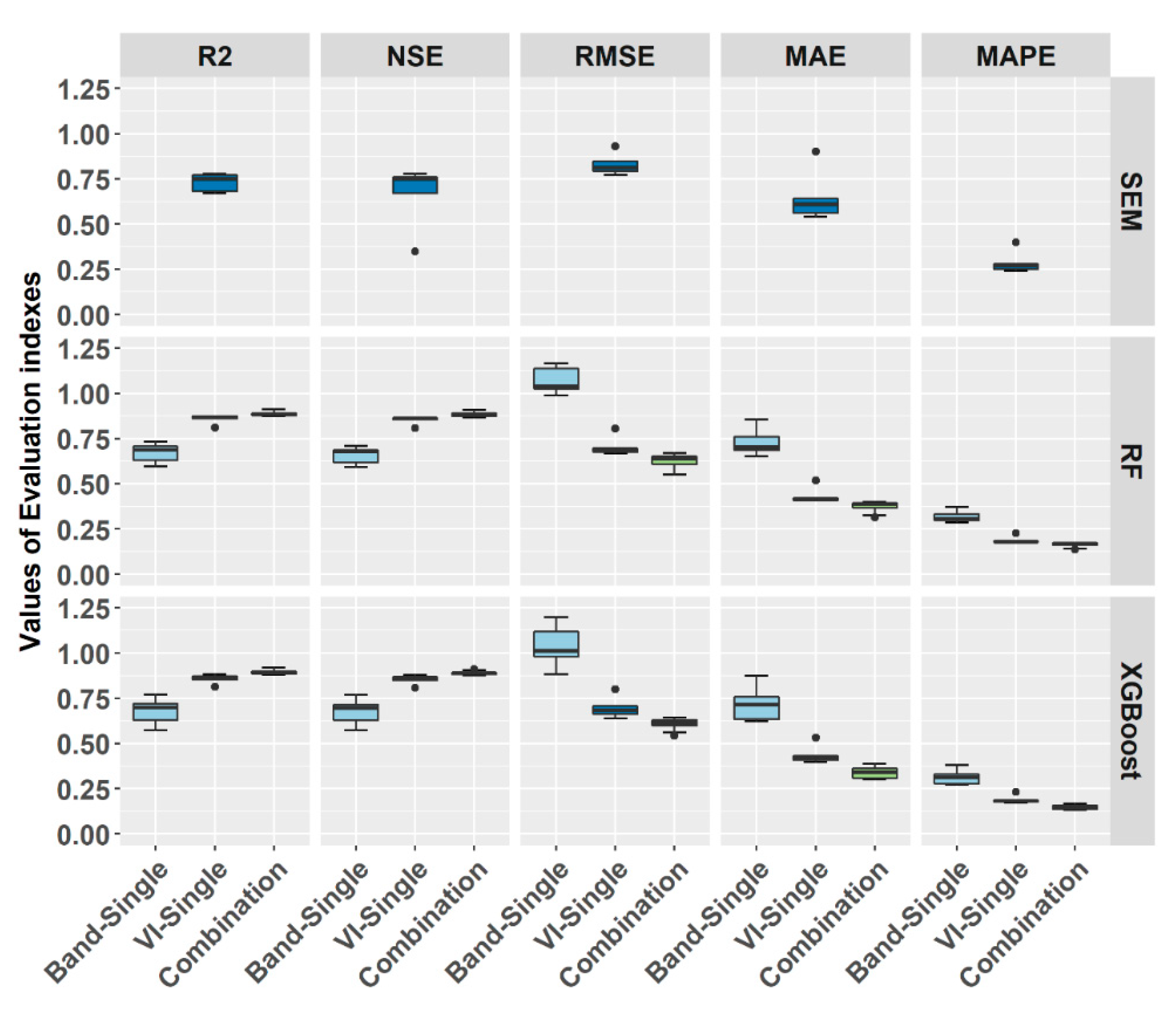
Moreover, our study also put all 10 bands and VIs as the input combination (ALL-10) for RF and XGBoost, which indicated that ALL-10 increased the accuracy slightly for RF compared with 2B + 5VI (Figure 12). For example, R2 and RMSE of ALL-10 were 0.911 and 0.551, while they were 0.906 and 0.568 of 2B + 5VI (Table 4). However, ALL-10 decreased the accuracy slightly for XGBoost compared with 2B + 5VI (Figure 12). The R2 and the RMSE of ALL-10 were 0.915 and 0.561, while they were 0.919 and 0.542 of 2B + 5VI for the XGBoost (Table 4). This is because the two models use different modeling methods. The RF model did not fully reflect the information of 2B + 5VIs, while the XGBoost model overcame the problem of increasing the band information and increasing the noise after eliminating the information of the NIR and the red bands [38,41]. In addition, our study also divided the statistical evaluation of each model for LAI estimation into three categories of only using a single band, a single VI, and band or VI combinations as input variables (Figure 13). Generally, the combinations (band, VI, or band + VI) had the highest estimation accuracy of LAI, followed by the single VI and the single band, which had the lowest accuracies. Meanwhile, for the single VI as an input variable, the machine learning models had higher accuracy than the SEM. Importantly, although the estimation accuracies of RF and XGBoost with different input variables were similar in the test process, we still propose that the XGBoost was more suitable for LAI estimation in our study. The main reason is that a big difference between the training and the test processes for the LAI estimation accuracy was found in RF (Tables S2–S4), which implied the over-fitting issue might occur in RF.
4. Conclusions
LAI is an important indicator of vegetation for crop growth and a vital variable for driving almost all agricultural and eco-hydrological models. This study established the rice LAI estimation models with different multispectral bands, VIs, and their combinations by XGBoost and compared the accuracy with RF and SEM models. The results indicated that the performance of multispectral bands and VIs for LAI estimation varied from different methods. The GNDVI had the highest LAI estimation accuracy in the SEM, and the NIR was the best band in both RF and XGBoost models. Meanwhile, NDRE and LCI performed better than other VIs in RF and XGBoost models, respectively. Band combination of NIR + red could improve the LAI estimation accuracy in both RF and XGBoost models, while adding more bands into the combination had little improvement for the LAI estimation accuracy. Similar to the band combinations, putting more than one VI together could only increase the LAI estimation accuracy slightly. Furthermore, our study found the bands + VIs combinations obtained higher LAI estimation accuracies in both RF and XGBoost models. Considering the potential over-fitting issue of RF, our study suggested using 2B + 5VI (red + NIR + OSAVI + NDVI + GNDVI + LCI + NDRE) to estimate the rice LAI by XGBoost. All bands and VIs could be easily obtained by the DJI Phantom 4 Multispectral (DJI-P4M, SZ DJI Technology Co., Ltd.), which is inexpensive and very convenient, increasing the practical value of this study.
Due to the limited parameters in RF and XGBoost, our study only calibrated the parameters manually by trial-and-error, making it difficult to obtain the global optimal solution. In the future, the automatic intelligent parameter optimization algorithms (e.g., bat algorithm, salp swarm algorithm) will be coupled with the XGBoost to further improve the estimation accuracy [39,66]. Moreover, the machine learning models could also be coupled with SEM or process-based methods to increase the universality of the model while improving the estimation accuracy.
Supplementary Materials
The following are available online at https://www.mdpi.com/article/10.3390/rs13183663/s1, Table S1: Parameters of RF and XGBoost with different inputs; Table S2: Statistical evaluation for the RF and XGBoost with multispectral bands (B) as input variables during the training period; Table S3: Statistical evaluation for the RF and XGBoost with vegetation indexes (VIs) as input variables during the training period; Table S4: Statistical evaluation for the RF and XGBoost with multispectral bands and vegetation indexes (VIs) as input variables during the training period.
Author Contributions
Conceptualization, W.Z. and L.W.; Formal analysis, S.L.; Funding acquisition, W.Z.; Investigation, S.L.; Methodology, G.L.; Software, S.L.; Writing—original draft, S.L. and W.Z.; Writing—review & editing, H.C., T.G., and A.K.S. All authors have read and agreed to the published version of the manuscript.
Funding
This research was funded by the National Key Research and Development Program of China (2019YFC0409203), the Program of the National Natural Science Foundation of China (NSFC) (Grant Nos. 51879196 and 51790533).
Institutional Review Board Statement
Not applicable.
Informed Consent Statement
Not applicable.
Data Availability Statement
Data used in this study are available from corresponding authors by request.
Acknowledgments
We thank Weipeng Yan and Zhuang Liu for their assistance in field sampling.
Conflicts of Interest
The authors declare no conflict of interest.
References
- Watson, D.J. Comparative Physiological Studies on the Growth of Field Crops: I. Variation in Net Assimilation Rate and Leaf Area between Species and Varieties, and within and between Years. Ann. Bot. 1947, 11, 41–76. [Google Scholar] [CrossRef]
- Brown, L.A.; Meier, C.; Morris, H.; Pastor-Guzman, J.; Bai, G.; Lerebourg, C.; Gobron, N.; Lanconelli, C.; Clerici, M.; Dash, J. Evaluation of global leaf area index and fraction of absorbed photosynthetically active radiation products over North America using Copernicus Ground Based Observations for Validation data. Remote Sens. Environ. 2020, 247, 111935. [Google Scholar] [CrossRef]
- Kanniah, K.; Kang, C.; Sharma, S.; Amir, A. Remote Sensing to Study Mangrove Fragmentation and Its Impacts on Leaf Area Index and Gross Primary Productivity in the South of Peninsular Malaysia. Remote Sens. 2021, 13, 1427. [Google Scholar] [CrossRef]
- Gan, R.; Zhang, Y.; Shi, H.; Yang, Y.; Eamus, D.; Cheng, L.; Chiew, F.H.; Yu, Q. Use of satellite leaf area index estimating evapotranspiration and gross assimilation for Australian ecosystems. Ecohydrol 2018, 11, e1974. [Google Scholar] [CrossRef]
- Lei, G.; Zeng, W.; Jiang, Y.; Ao, C.; Wu, J.; Huang, J. Sensitivity analysis of the SWAP (Soil-Water-Atmosphere-Plant) model under different nitrogen applications and root distributions in saline soils. Pedosphere 2021, 31, 807–821. [Google Scholar] [CrossRef]
- Zhu, J.; Zeng, W.; Ma, T.; Lei, G.; Zha, Y.; Fang, Y.; Wu, J.; Huang, J. Testing and Improving the WOFOST Model for Sunflower Simulation on Saline Soils of Inner Mongolia, China. Agronomy 2018, 8, 172. [Google Scholar] [CrossRef] [Green Version]
- Zeng, W.; Xu, C.; Wu, J.; Huang, J. Sunflower seed yield estimation under the interaction of soil salinity and nitrogen application. Field Crop. Res. 2016, 198, 1–15. [Google Scholar] [CrossRef]
- Jonckheere, I.; Fleck, S.; Nackaerts, K.; Muys, B.; Coppin, P.; Weiss, M.; Baret, F. Review of methods for in situ leaf area index determination: Part, I. Theories, sensors and hemispherical photography. Agric. For. Meteorol. 2004, 121, 19–35. [Google Scholar] [CrossRef]
- Chen, Y.; Zhang, Z.; Tao, F. Improving regional winter wheat yield estimation through assimilation of phenology and leaf area index from remote sensing data. Eur. J. Agron. 2018, 101, 163–173. [Google Scholar] [CrossRef]
- Srinet, R.; Nandy, S.; Patel, N. Estimating leaf area index and light extinction coefficient using Random Forest regression algorithm in a tropical moist deciduous forest, India. Ecol. Informatics 2019, 52, 94–102. [Google Scholar] [CrossRef]
- Bsaibes, A.; Courault, D.; Baret, F.; Weiss, M.; Olioso, A.; Jacob, F.; Hagolle, O.; Marloie, O.; Bertrand, N.; Desfond, V.; et al. Albedo and LAI estimates from FORMOSAT-2 data for crop monitoring. Remote Sens. Environ. 2009, 113, 716–729. [Google Scholar] [CrossRef]
- Qu, Y.; Han, W.; Ma, M. Retrieval of a Temporal High-Resolution Leaf Area Index (LAI) by Combining MODIS LAI and ASTER Reflectance Data. Remote Sens. 2014, 7, 195–210. [Google Scholar] [CrossRef]
- Jafari, M.; Keshavarz, A. Improving CERES-Wheat Yield Forecasts by Assimilating Dynamic Landsat-Based Leaf Area Index: A Case Study in Iran. J. Indian Soc. Remote Sens. 2021, 1–14. [Google Scholar] [CrossRef]
- Dehkordi, R.H.; Denis, A.; Fouche, J.; Burgeon, V.; Cornelis, J.T.; Tychon, B.; Gomez, E.P.; Meersmans, J. Remotely-sensed assessment of the impact of century-old biochar on chicory crop growth using high-resolution UAV-based imagery. Int. J. Appl. Earth Obs. Geoinf. 2020, 91, 102147. [Google Scholar] [CrossRef]
- Zhang, M.; Zhou, J.; Sudduth, K.A.; Kitchen, N.R. Estimation of maize yield and effects of variable-rate nitrogen application using UAV-based RGB imagery. Biosyst. Eng. 2020, 189, 24–35. [Google Scholar] [CrossRef]
- Yuan, M.; Burjel, J.C.; Martin, N.F.; Isermann, J.; Goeser, N.; Pittelkow, C.M. Advancing on-farm research with UAVs: Cover crop effects on crop growth and yield. Agron. J. 2021, 113, 1071–1083. [Google Scholar] [CrossRef]
- Tao, H.; Feng, H.; Xu, L.; Miao, M.; Long, H.; Yue, J.; Li, Z.; Yang, G.; Yang, X.; Fan, L. Estimation of Crop Growth Parameters Using UAV-Based Hyperspectral Remote Sensing Data. Sensors 2020, 20, 1296. [Google Scholar] [CrossRef] [Green Version]
- Barbosa, B.; Ferraz, G.A.E.S.; dos Santos, L.M.; Santana, L.; Marin, D.B.; Rossi, G.; Conti, L. Application of RGB Images Obtained by UAV in Coffee Farming. Remote Sens. 2021, 13, 2397. [Google Scholar] [CrossRef]
- Apolo-Apolo, O.E.; Pérez-Ruiz, M.; Martínez-Guanter, J.; Egea, G. A Mixed Data-Based Deep Neural Network to Estimate Leaf Area Index in Wheat Breeding Trials. Agronomy 2020, 10, 175. [Google Scholar] [CrossRef] [Green Version]
- Demarez, V.; Duthoit, S.; Baret, F.; Weiss, M.; Dedieu, G. Estimation of leaf area and clumping indexes of crops with hemispherical photographs. Agric. For. Meteorol. 2008, 148, 644–655. [Google Scholar] [CrossRef] [Green Version]
- Ahmad, S.; Ali, H.; Ur Rehman, A.; Khan, R.J.Z.; Ahmad, W.; Fatima, Z.; Abbas, G.; Irfan, M.; Ali, H.; Khan, M.A. Measuring leaf area of winter cereals by different techniques: A comparison. Pak. J. Life Soc. Sci 2015, 13, 117–125. [Google Scholar]
- Yao, X.; Wang, N.; Liu, Y.; Cheng, T.; Tian, Y.; Chen, Q.; Zhu, Y. Estimation of Wheat LAI at Middle to High Levels Using Unmanned Aerial Vehicle Narrowband Multispectral Imagery. Remote Sens. 2017, 9, 1304. [Google Scholar] [CrossRef] [Green Version]
- Qi, H.; Zhu, B.; Wu, Z.; Liang, Y.; Li, J.; Wang, L.; Chen, T.; Lan, Y.; Zhang, L. Estimation of Peanut Leaf Area Index from Unmanned Aerial Vehicle Multispectral Images. Sensors 2020, 20, 6732. [Google Scholar] [CrossRef]
- Peñuelas, J.; Isla, R.; Filella, I.; Araus, J.L. Visible and Near-Infrared Reflectance Assessment of Salinity Effects on Barley. Crop. Sci. 1997, 37, 198–202. [Google Scholar] [CrossRef]
- Huete, A. A soil-adjusted vegetation index (SAVI). Remote Sens. Environ. 1988, 25, 295–309. [Google Scholar] [CrossRef]
- Steven, M.D. The Sensitivity of the OSAVI Vegetation Index to Observational Parameters. Remote Sens. Environ. 1998, 63, 49–60. [Google Scholar] [CrossRef]
- Du, C.; Meng, Q.; Qin, Q.; Dong, H. The development of a new model on vegetation water content. In Proceedings of the 2013 IEEE International Geoscience and Remote Sensing Symposium-IGARSS, Melbourne, Australia, 21–26 July 2013. [Google Scholar] [CrossRef]
- Miura, T.; Huete, A.R.; Yoshioka, H.; Holben, B.N. An error and sensitivity analysis of atmospheric resistant vegetation indices derived from dark target-based atmospheric correction. Remote Sens. Environ. 2001, 78, 284–298. [Google Scholar] [CrossRef]
- Jiang, Z.; Huete, A.R.; Didan, K.; Miura, T. Development of a two-band enhanced vegetation index without a blue band. Remote Sens. Environ. 2008, 112, 3833–3845. [Google Scholar] [CrossRef]
- Stamatiadis, S.; Taskos, D.; Tsadilas, C.; Christofides, C.; Tsadila, E.; Schepers, J.S. Relation of Ground-Sensor Canopy Reflectance to Biomass Production and Grape Color in Two Merlot Vineyards. Am. J. Enol. Vitic. 2006, 57, 415–422. [Google Scholar]
- Liu, C.; Shan, Y.; Nepf, H. Impact of Stem Size on Turbulence and Sediment Resuspension Under Unidirectional Flow. Water Resour. Res. 2021, 57, e2020WR028620. [Google Scholar] [CrossRef]
- Box, W.; Järvelä, J.; Västilä, K. Flow resistance of floodplain vegetation mixtures for modelling river flows. J. Hydrol. 2021, 601, 126593. [Google Scholar] [CrossRef]
- Lama, G.; Crimaldi, M.; Pasquino, V.; Padulano, R.; Chirico, G. Bulk Drag Predictions of Riparian Arundo donax Stands through UAV-Acquired Multispectral Images. Water 2021, 13, 1333. [Google Scholar] [CrossRef]
- Peng, X.; Han, W.; Ao, J.; Wang, Y. Assimilation of LAI Derived from UAV Multispectral Data into the SAFY Model to Estimate Maize Yield. Remote Sens. 2021, 13, 1094. [Google Scholar] [CrossRef]
- Dong, T.; Liu, J.; Shang, J.; Qian, B.; Ma, B.; Kovacs, J.M.; Walters, D.; Jiao, X.; Geng, X.; Shi, Y. Assessment of red-edge vegetation indices for crop leaf area index estimation. Remote Sens. Environ. 2019, 222, 133–143. [Google Scholar] [CrossRef]
- Gahrouei, O.R.; McNairn, H.; Hosseini, M.; Homayouni, S. Estimation of Crop Biomass and Leaf Area Index from Multitemporal and Multispectral Imagery Using Machine Learning Approaches. Can. J. Remote Sens. 2020, 46, 84–99. [Google Scholar] [CrossRef]
- Maimaitijiang, M.; Sagan, V.; Sidike, P.; Daloye, A.M.; Erkbol, H.; Fritschi, F.B. Crop Monitoring Using Satellite/UAV Data Fusion and Machine Learning. Remote Sens. 2020, 12, 1357. [Google Scholar] [CrossRef]
- Chen, T.; Guestrin, C. XGBoost: A Scalable Tree Boosting System. In Proceedings of the 22nd ACM SIGKDD International Conference on Knowledge Discovery and Data Mining, San Francisco, CA, USA, 13–17 August 2016; pp. 785–794. [Google Scholar]
- Han, Y.; Wu, J.; Zhai, B.; Pan, Y.; Huang, G.; Wu, L.; Zeng, W. Coupling a Bat Algorithm with XGBoost to Estimate Reference Evapotranspiration in the Arid and Semiarid Regions of China. Adv. Meteorol. 2019, 2019, 1–16. [Google Scholar] [CrossRef]
- Fan, J.; Wu, L.; Ma, X.; Zhou, H.; Zhang, F. Hybrid support vector machines with heuristic algorithms for prediction of daily diffuse solar radiation in air-polluted regions. Renew. Energy 2020, 145, 2034–2045. [Google Scholar] [CrossRef]
- Fan, J.; Wu, L.; Zhang, F.; Cai, H.; Zeng, W.; Wang, X.; Zou, H. Empirical and machine learning models for predicting daily global solar radiation from sunshine duration: A review and case study in China. Renew. Sustain. Energy Rev. 2019, 100, 186–212. [Google Scholar] [CrossRef]
- Setyawan, T.A.; Riwinanto, S.A.; Suhendro; Helmy; Nursyahid, A.; Nugroho, A.S. Comparison of HSV and LAB Color Spaces for Hydroponic Monitoring System. In Proceedings of the 2018 5th International Conference on Information Technology, Computer, and Electrical Engineering (ICITACEE), Hotel Santika Premier, Indonesia, 26–28 September 2018; pp. 347–352. [Google Scholar]
- Tang, H.; Brolly, M.; Zhao, F.; Strahler, A.H.; Schaaf, C.L.; Ganguly, S.; Zhang, G.; Dubayah, R. Deriving and validating Leaf Area Index (LAI) at multiple spatial scales through lidar remote sensing: A case study in Sierra National Forest, CA. Remote Sens. Environ. 2014, 143, 131–141. [Google Scholar] [CrossRef]
- Myung, J.; Lee, W. Adaptive Binary Splitting: A RFID Tag Collision Arbitration Protocol for Tag Identification. Mob. Networks Appl. 2006, 11, 711–722. [Google Scholar] [CrossRef]
- Dorafshan, S.; Thomas, R.J.; Maguire, M. Comparison of deep convolutional neural networks and edge detectors for image-based crack detection in concrete. Construct. Build. Mater. 2018, 186, 1031–1045. [Google Scholar] [CrossRef]
- Liu, J.; Pattey, E.; Jégo, G. Assessment of vegetation indices for regional crop green LAI estimation from Landsat images over multiple growing seasons. Remote Sens. Environ. 2012, 123, 347–358. [Google Scholar] [CrossRef]
- Jin, H.; Eklundh, L. A physically based vegetation index for improved monitoring of plant phenology. Remote Sens. Environ. 2014, 152, 512–525. [Google Scholar] [CrossRef]
- Xiao, J.; Davis, K.J.; Urban, N.M.; Keller, K. Uncertainty in model parameters and regional carbon fluxes: A model-data fusion approach. Agric. For. Meteorol. 2014, 189–190, 175–186. [Google Scholar] [CrossRef]
- Breiman, L. Random Forests. Mach. Learn. 2001, 45, 5–32. [Google Scholar] [CrossRef] [Green Version]
- Dewi, C.; Chen, R.-C. Random forest and support vector machine on features selection for regression analysis. Int. J. Innov. Comput. Inf. Control. 2019, 15, 2027–2037. [Google Scholar] [CrossRef]
- Kearns, M.; Valiant, L. Cryptographic limitations on learning Boolean formulae and finite automata. J. ACM 1994, 41, 67–95. [Google Scholar] [CrossRef]
- Zhang, C.; Wang, D.; Song, C.; Wang, L.; Song, J.; Guan, L.; Zhang, M. Interpretable Learning Algorithm Based on XGBoost for Fault Prediction in Optical Network. In Proceedings of the Optical Fiber Communication Conference (OFC), San Diego, CA, USA, 8–12 March 2020. [Google Scholar]
- Gonsamo, A. Leaf area index retrieval using gap fractions obtained from high resolution satellite data: Comparisons of approaches, scales and atmospheric effects. Int. J. Appl. Earth Obs. Geoinf. 2010, 12, 233–248. [Google Scholar] [CrossRef]
- Li, H.; Liu, G.; Liu, Q.; Chen, Z.; Huang, C. Retrieval of Winter Wheat Leaf Area Index from Chinese GF-1 Satellite Data Using the PROSAIL Model. Sensors 2018, 18, 1120. [Google Scholar] [CrossRef] [PubMed] [Green Version]
- Wang, F.-M.; Huang, J.-F.; Tang, Y.-L.; Wang, X.-Z. New Vegetation Index and Its Application in Estimating Leaf Area Index of Rice. Rice Sci. 2007, 14, 195–203. [Google Scholar] [CrossRef]
- Milas, A.S.; Romanko, M.; Reil, P.; Abeysinghe, T.; Marambe, A. The importance of leaf area index in mapping chlorophyll content of corn under different agricultural treatments using UAV images. Int. J. Remote Sens. 2018, 39, 5415–5431. [Google Scholar] [CrossRef]
- Li, F.; Miao, Y.; Feng, G.; Yuan, F.; Yue, S.; Gao, X.; Liu, Y.; Liu, B.; Ustin, S.L.; Chen, X. Improving estimation of summer maize nitrogen status with red edge-based spectral vegetation indices. Field Crop. Res. 2014, 157, 111–123. [Google Scholar] [CrossRef]
- Zhang, K.; Ge, X.; Shen, P.; Li, W.; Liu, X.; Cao, Q.; Zhu, Y.; Cao, W.; Tian, Y. Predicting Rice Grain Yield Based on Dynamic Changes in Vegetation Indexes during Early to Mid-Growth Stages. Remote Sens. 2019, 11, 387. [Google Scholar] [CrossRef] [Green Version]
- Peng, Y.; Nguy-Robertson, A.; Arkebauer, T.; Gitelson, A.A. Assessment of Canopy Chlorophyll Content Retrieval in Maize and Soybean: Implications of Hysteresis on the Development of Generic Algorithms. Remote Sens. 2017, 9, 226. [Google Scholar] [CrossRef] [Green Version]
- Tucker, C.J. Red and photographic infrared linear combinations for monitoring vegetation. Remote Sens. Environ. 1979, 8, 127–150. [Google Scholar] [CrossRef] [Green Version]
- Molnár, V.É.; Simon, E.; Tóthmérész, B.; Ninsawat, S.; Szabó, S. Air pollution induced vegetation stress—The Air Pollution Tolerance Index as a quick tool for city health evaluation. Ecol. Indic. 2020, 113, 106234. [Google Scholar] [CrossRef]
- Fan, J.; Wang, X.; Wu, L.; Zhou, H.; Zhang, F.; Yu, X.; Lu, X.; Xiang, Y. Comparison of Support Vector Machine and Extreme Gradient Boosting for predicting daily global solar radiation using temperature and precipitation in humid subtropical climates: A case study in China. Energy Convers. Manag. 2018, 164, 102–111. [Google Scholar] [CrossRef]
- Myneni, R.; Williams, D. On the relationship between FAPAR and NDVI. Remote Sens. Environ. 1994, 49, 200–211. [Google Scholar] [CrossRef]
- Antipov, E.A.; Pokryshevskaya, E.B. Mass appraisal of residential apartments: An application of Random forest for valuation and a CART-based approach for model diagnostics. Expert Syst. Appl. 2012, 39, 1772–1778. [Google Scholar] [CrossRef] [Green Version]
- Zarco-Tejada, P.; Miller, J.; Morales, A.; Berjón, A.; Agüera-Vega, J. Hyperspectral indices and model simulation for chlorophyll estimation in open-canopy tree crops. Remote Sens. Environ. 2004, 90, 463–476. [Google Scholar] [CrossRef]
- Wang, H.; Yan, H.; Zeng, W.; Lei, G.; Ao, C.; Zha, Y. A novel nonlinear Arps decline model with salp swarm algorithm for predicting pan evaporation in the arid and semi-arid regions of China. J. Hydrol. 2020, 582, 124545. [Google Scholar] [CrossRef]
Figure 1.
Location of the study site (a) and the experimental fields (b,c). (b) is the visible image (RGB) and (c) is the NDVI image, both taken on 26 June 2020.
Figure 1.
Location of the study site (a) and the experimental fields (b,c). (b) is the visible image (RGB) and (c) is the NDVI image, both taken on 26 June 2020.

Figure 2.
Framework for determining rice leaf area of a single plant (LAS) and plant density (PD) from the multispectral images. ITS indicates image threshold segmentation.
Figure 2.
Framework for determining rice leaf area of a single plant (LAS) and plant density (PD) from the multispectral images. ITS indicates image threshold segmentation.

Figure 3.
Framework of the random forest model (RF).

Figure 4.
Framework of the Extreme Gradient Boosting model (XGBoost). fn-1(X,Y) and fn(X,Y) are the predicted values for n and n-1 iterations.
Figure 4.
Framework of the Extreme Gradient Boosting model (XGBoost). fn-1(X,Y) and fn(X,Y) are the predicted values for n and n-1 iterations.

Figure 5.
Relationship between the observed and estimated leaf area index (LAI) of rice by Semi-Empirical Model (SEM) with vegetation indexes (VIs) in the test process. Dash lines and red solid lines are the 1:1 lines and linear fitting lines respectively. The shaded areas indicate the range of 95% prediction bands.

Figure 6.
Relationship between observed and estimated leaf area index (LAI) of rice by random forest model (RF) with multispectral bands (B) in the test process. Dash lines and red solid lines are the 1:1 lines and the linear fitting lines, respectively. The shaded areas indicate the range of 95% prediction bands.

Figure 7.
Important feature selection analysis with multispectral bands (B) as input variables by random forest model (RF, a) and Extreme Gradient Boosting model (XGBoost, b). IncMSE is the order of increase in mean square error, and IncNodePurity is the increase in node purity.
Figure 7.
Important feature selection analysis with multispectral bands (B) as input variables by random forest model (RF, a) and Extreme Gradient Boosting model (XGBoost, b). IncMSE is the order of increase in mean square error, and IncNodePurity is the increase in node purity.

Figure 8.
Relationship between observed and estimated leaf area index (LAI) of rice by Extreme Gradient Boosting model (XGBoost) with multispectral bands (B) in the test process. Dash lines and red solid lines are the 1:1 lines and the linear fitting lines, respectively. The shaded areas indicate the range of 95% prediction bands.

Figure 9.
Relationship between observed and estimated leaf area index (LAI) of rice by random forest model (RF) with vegetation indexes (VIs) in the test process. Dash lines and red solid lines are the 1:1 lines and the linear fitting lines, respectively. The shaded areas indicate the range of 95% prediction bands.

Figure 10.
Important feature selection analysis with vegetation indexes (VIs) as input variables by random forest model (RF, a) and Extreme Gradient Boosting model (XGBoost, b). IncMSE is the order of increase in mean square error, and IncNodePurity is the increase in node purity.
Figure 10.
Important feature selection analysis with vegetation indexes (VIs) as input variables by random forest model (RF, a) and Extreme Gradient Boosting model (XGBoost, b). IncMSE is the order of increase in mean square error, and IncNodePurity is the increase in node purity.

Figure 11.
Relationship between observed and estimated leaf area index (LAI) of rice by Extreme Gradient Boosting model (XGBoost) with vegetation indexes (VIs) in the test process. Dash lines and red solid lines are the 1:1 lines and the linear fitting lines, respectively. The shaded areas indicate the range of 95% prediction bands.

Figure 12.
Relationship between observed and estimated leaf area index (LAI) of rice by random forest model (RF) and Extreme Gradient Boosting model (XGBoost) with multispectral bands (B) and vegetation indexes (VIs) in the test process. Dash lines and red solid lines are the 1:1 lines and the linear fitting lines, respectively. The shaded areas indicate the range of 95% prediction bands.

Figure 13.
Boxplot for the estimation accuracy of leaf area index (LAI) with band, vegetation index (VI), and their combinations as input variables. The horizontal line in the box is the median, the ends of the box are the lower hinge (25th percentile, Q1) and the upper hinge (75th percentile, Q3), and the whiskers extend to 1.5× (Q3–Q1), beyond which outliers are indicated by a black dot.


Table 1.
Parameters and statistical indexes of leaf area index (LAI) semi-empirical model (SEM) for the vegetation indexes (VIs) inversion.
Table 1.
Parameters and statistical indexes of leaf area index (LAI) semi-empirical model (SEM) for the vegetation indexes (VIs) inversion.
| Vegetation Indexes (VIs) | Training Process | Test Process | |||||
|---|---|---|---|---|---|---|---|
| KVI | VI∞ | RMSE | R2 | MAE | NSE | MAPE | |
| GNDVI | 0.899 | 0.95 | 0.77 | 0.78 | 0.54 | 0.78 | 0.24 |
| LCI | 0.731 | 0.86 | 0.8 | 0.77 | 0.56 | 0.76 | 0.25 |
| NDRE | 0.419 | 0.66 | 1.31 | 0.67 | 0.9 | 0.35 | 0.4 |
| NDVI | 0.285 | 0.573 | 0.82 | 0.75 | 0.61 | 0.75 | 0.27 |
| OSAVI | 0.391 | 0.54 | 0.93 | 0.68 | 0.64 | 0.67 | 0.28 |
Table 2.
Statistical evaluation for RF and XGBoost with multispectral bands (B) as input variables.
| Model Type | RF | XGBoost | |||
|---|---|---|---|---|---|
| Inputs | Red + NIR + OSAVI + NDVI + GNDVI + LCI + NDRE | ALL-10 | Red + NIR + OSAVI + NDVI + GNDVI + LCI + NDRE | ALL-10 | |
| Evaluation Indices | RMSE | 0.568 | 0.551 | 0.542 | 0.561 |
| R2 | 0.906 | 0.911 | 0.919 | 0.915 | |
| MAE | 0.326 | 0.314 | 0.3 | 0.301 | |
| NSE | 0.904 | 0.909 | 0.912 | 0.906 | |
| MAPE | 0.142 | 0.137 | 0.131 | 0.131 | |
Table 3.
Statistical evaluation for RF and XGBoost with vegetation indexes (VIs) as input variables.
Table 3.
Statistical evaluation for RF and XGBoost with vegetation indexes (VIs) as input variables.
| Bands (B) | RF | XGBoost | ||||||||
|---|---|---|---|---|---|---|---|---|---|---|
| RMSE | R2 | MAE | NSE | MAPE | RMSE | R2 | MAE | NSE | MAPE | |
| Red | 1.039 | 0.706 | 0.652 | 0.679 | 0.284 | 0.980 | 0.720 | 0.622 | 0.714 | 0.271 |
| Blue | 1.136 | 0.629 | 0.761 | 0.616 | 0.332 | 1.119 | 0.630 | 0.756 | 0.627 | 0.330 |
| Green | 1.025 | 0.688 | 0.702 | 0.687 | 0.306 | 1.012 | 0.698 | 0.714 | 0.695 | 0.311 |
| NIR | 0.988 | 0.733 | 0.686 | 0.709 | 0.299 | 0.881 | 0.771 | 0.636 | 0.769 | 0.277 |
| RE | 1.167 | 0.596 | 0.855 | 0.594 | 0.372 | 1.197 | 0.574 | 0.874 | 0.573 | 0.381 |
| Red + NIR | 0.655 | 0.875 | 0.392 | 0.872 | 0.171 | 0.636 | 0.883 | 0.377 | 0.879 | 0.164 |
| Red + Green + NIR | 0.644 | 0.877 | 0.396 | 0.876 | 0.173 | 0.610 | 0.894 | 0.340 | 0.889 | 0.148 |
| Red + Blue + Green + NIR | 0.638 | 0.879 | 0.399 | 0.879 | 0.174 | 0.596 | 0.900 | 0.316 | 0.894 | 0.138 |
| Red + Blue + Green + NIR + RE | 0.612 | 0.889 | 0.369 | 0.889 | 0.161 | 0.603 | 0.896 | 0.307 | 0.892 | 0.134 |
Table 4.
Statistical evaluation for RF and XGBoost with multispectral bands and vegetation indexes (VIs) as input variables.
Table 4.
Statistical evaluation for RF and XGBoost with multispectral bands and vegetation indexes (VIs) as input variables.
| Vegetation Indexes (VIs) | RF | XGBoost | ||||||||
|---|---|---|---|---|---|---|---|---|---|---|
| RMSE | R2 | MAE | NSE | MAPE | RMSE | R2 | MAE | NSE | MAPE | |
| NDVI | 0.696 | 0.861 | 0.412 | 0.856 | 0.179 | 0.708 | 0.853 | 0.431 | 0.851 | 0.188 |
| GNDVI | 0.685 | 0.868 | 0.410 | 0.860 | 0.178 | 0.682 | 0.866 | 0.418 | 0.862 | 0.182 |
| LCI | 0.675 | 0.874 | 0.420 | 0.864 | 0.183 | 0.637 | 0.881 | 0.397 | 0.879 | 0.173 |
| NDRE | 0.667 | 0.875 | 0.409 | 0.867 | 0.178 | 0.663 | 0.872 | 0.409 | 0.869 | 0.178 |
| OSAVI | 0.804 | 0.811 | 0.519 | 0.808 | 0.226 | 0.800 | 0.813 | 0.532 | 0.809 | 0.232 |
| LCI + NDRE | 0.661 | 0.878 | 0.400 | 0.870 | 0.174 | 0.643 | 0.879 | 0.388 | 0.877 | 0.169 |
| GNDVI + LCI + NDRE | 0.669 | 0.877 | 0.387 | 0.867 | 0.169 | 0.633 | 0.884 | 0.365 | 0.880 | 0.159 |
| NDVI + GNDVI + LCI + NDRE | 0.640 | 0.887 | 0.391 | 0.878 | 0.170 | 0.617 | 0.890 | 0.341 | 0.886 | 0.148 |
| OSAVI + NDVI + GNDVI + LCI + NDRE | 0.608 | 0.892 | 0.365 | 0.890 | 0.159 | 0.621 | 0.889 | 0.352 | 0.885 | 0.153 |
Publisher’s Note: MDPI stays neutral with regard to jurisdictional claims in published maps and institutional affiliations. |
© 2021 by the authors. Licensee MDPI, Basel, Switzerland. This article is an open access article distributed under the terms and conditions of the Creative Commons Attribution (CC BY) license (https://creativecommons.org/licenses/by/4.0/).
Share and Cite
MDPI and ACS Style
Liu, S.; Zeng, W.; Wu, L.; Lei, G.; Chen, H.; Gaiser, T.; Srivastava, A.K. Simulating the Leaf Area Index of Rice from Multispectral Images. Remote Sens. 2021, 13, 3663. https://doi.org/10.3390/rs13183663
AMA Style
Liu S, Zeng W, Wu L, Lei G, Chen H, Gaiser T, Srivastava AK. Simulating the Leaf Area Index of Rice from Multispectral Images. Remote Sensing. 2021; 13(18):3663. https://doi.org/10.3390/rs13183663
Chicago/Turabian StyleLiu, Shenzhou, Wenzhi Zeng, Lifeng Wu, Guoqing Lei, Haorui Chen, Thomas Gaiser, and Amit Kumar Srivastava. 2021. "Simulating the Leaf Area Index of Rice from Multispectral Images" Remote Sensing 13, no. 18: 3663. https://doi.org/10.3390/rs13183663
Note that from the first issue of 2016, this journal uses article numbers instead of page numbers. See further details here.