
Remote Sensing of Wetlands in the Prairie Pothole Region of North America
by
 ,
,
Joshua Montgomery
1,*, 
Craig Mahoney
1,
Brian Brisco
2 ,
,
Lyle Boychuk
3,
Danielle Cobbaert
1 and
Chris Hopkinson
4 1
Alberta Environment and Parks, 9888 Jasper Avenue, Edmonton, AB T5J 5C6, Canada
2
Canada Centre for Mapping and Earth Observation, 588 Booth St., Ottawa, ON K1A 0Y7, Canada
3
Prairie Region, Ducks Unlimited Canada, 1030 Winnipeg St., Regina, SK S4R 8P8, Canada
4
Department of Geography, University of Lethbridge, 4401 University Drive, Lethbridge, AB T1K3M4, Canada
*
Author to whom correspondence should be addressed.
Remote Sens. 2021, 13(19), 3878; https://doi.org/10.3390/rs13193878
Submission received: 2 July 2021
/
Revised: 14 September 2021
/
Accepted: 19 September 2021
/
Published: 28 September 2021
(This article belongs to the Special Issue Remote Sensing of Wetland Vegetation Patterns and Dynamics)
Abstract
:The Prairie Pothole Region (PPR) of North America is an extremely important habitat for a diverse range of wetland ecosystems that provide a wealth of socio-economic value. This paper describes the ecological characteristics and importance of PPR wetlands and the use of remote sensing for mapping and monitoring applications. While there are comprehensive reviews for wetland remote sensing in recent publications, there is no comprehensive review about the use of remote sensing in the PPR. First, the PPR is described, including the wetland classification systems that have been used, the water regimes that control the surface water and water levels, and the soil and vegetation characteristics of the region. The tools and techniques that have been used in the PPR for analyses of geospatial data for wetland applications are described. Field observations for ground truth data are critical for good validation and accuracy assessment of the many products that are produced. Wetland classification approaches are reviewed, including Decision Trees, Machine Learning, and object versus pixel-based approaches. A comprehensive description of the remote sensing systems and data that have been employed by various studies in the PPR is provided. A wide range of data can be used for various applications, including passive optical data like aerial photographs or satellite-based, Earth-observation data. Both airborne and spaceborne lidar studies are described. A detailed description of Synthetic Aperture RADAR (SAR) data and research are provided. The state of the art is the use of multi-source data to achieve higher accuracies and hybrid approaches. Digital Surface Models are also being incorporated in geospatial analyses to separate forest and shrub and emergent systems based on vegetation height. Remote sensing provides a cost-effective mechanism for mapping and monitoring PPR wetlands, especially with the logistical difficulties and cost of field-based methods. The wetland characteristics of the PPR dictate the need for high resolution in both time and space, which is increasingly possible with the numerous and increasing remote sensing systems available and the trend to open-source data and tools. The fusion of multi-source remote sensing data via state-of-the-art machine learning is recommended for wetland applications in the PPR. The use of such data promotes flexibility for sensor addition, subtraction, or substitution as a function of application needs and potential cost restrictions. This is important in the PPR because of the challenges related to the highly dynamic nature of this unique region.
1. Introduction and Background
Wetlands are a known provider of substantial economic, environmental and social value through a host of vital services [1]. For example, wetlands play a crucial role in the replenishment and storage of groundwater [2,3], not only serving as natural water retention ponds that prevent flooding and erosion [4,5] but also by filtering and purifying water [6,7]. Furthermore, wetlands directly influence wet area and riparian vegetation zone extents [8], hydrological regimes [9], and biodiversity [10]. In addition, wetlands often provide locations for human recreation and incubate socio-cultural values through hunting and gathering activities within native communities [11]. Wetlands have also been found to play a significant role in climate change mitigation [12,13,14,15]. Despite their known value, wetland ecosystems are declining at an unprecedented rate, particularly in regions undergoing development [16]. One such region is the Prairie Pothole Region (PPR) of North America.
The PPR encompasses an area of approximately 777,000 km2 in the northern Great Plains of North America that extends from Iowa through the Dakotas in the United States (US), into the Canadian provinces of Manitoba, Saskatchewan, and Alberta [17] (Figure 1). The PPR is predominantly a series of gently rolling plains dominated by agricultural activities and modified grasslands. Prairie potholes are depressions formed after glacial retreat in the last ice age, approximately 12,000 years ago [18,19]. The majority of wetlands in the PPR are mineral wetlands that form due to frequent, seasonally fluctuating water levels [20] that pool in depressions, promoting the formation of wetlands that are highly variable in size and permanency [19]. Most PPR wetlands exist as isolated (or closed) basins that only connect within a hydrological system during wet conditions when depressions reach ‘bank-full’ conditions and begin to spill into adjacent depressions, known as the ‘fill and spill’ mechanism [21]. The limited amount of organic matter, dry conditions, and shallow topsoil in the PPR generally discourages the formation of peaty organic substrates. In North America, wetlands that form in the PPR provide important habitat for waterfowl [22,23] and migrating birds [24,25]. It is estimated that PPR wetlands provide habitat to one-third of all Canada’s bird species at risk [26,27,28]. In addition, prairie pothole wetlands are highly productive nutrient sinks [29,30] and provide flood attenuation and purification, as well as water storage [4].
Wetlands in the PPR were first classified by Stewart and Kantrud [26] and Cowardin et al. [31] as marsh and open water wetlands. Marshes in the PPR are commonly located between uplands and open water. Within Alberta, shallow open-water (SOW) wetlands (i.e., less than 2 m depth) [32] are identified separately from open water wetlands (permanent lakes under the Stewart and Kantrud [26] classification system) and are typically located between marshes and deep-water bodies. Many of the pothole wetlands are ephemeral and highly variable in size and permanency [33] as a result of varying water levels related to source availability from precipitation, runoff, groundwater, and streams. Many PPR wetlands have a water depth of <1 m at peak volume; water level and surface water extent can fluctuate daily, seasonally, and unpredictably following prolonged periods of rainfall or (conversely) drought, affecting the wetland’s ecological characteristics [34,35]. In some cases, a sufficient reduction in water level can expose mudflats and alkaline soil. Conversely, floating and/or submerged vegetation may occur in nutrient-rich wetlands when water depths are too great for emergent vegetation to establish [36]. The temporal longevity of wetlands on the prairie landscape varies dramatically. Some are present during peak saturation only (temporary), others exist for the duration of the growing/wet season and sometimes beyond (seasonal to semi-permanent), whereas others are permanent [37]. Typically, temporary or seasonal wetlands are most abundant across the southern prairies of the Alberta PPR, thus making them sensitive to multi-year climate cycles, such as El Niño-southern oscillation (ENSO) events [31]. Therefore, pothole wetlands in the PPR are especially sensitive to natural climatic variability, human-induced climate change, and human modification of land-surface hydrology (e.g., ditches and draining), making them one of the most dynamic hydrological systems in the world [38].
Figure 1.
Extent of the Prairie Pothole Region in North America. Polygon is based on delineation from Mann [39].
Figure 1.
Extent of the Prairie Pothole Region in North America. Polygon is based on delineation from Mann [39].

Changes in the water balance of PPR wetlands are predominantly driven by changes in the input (precipitation) and the primary output (actual evapotranspiration; AET), which is driven by a range of hydrometeorological and land cover factors [40,41]. Water loss in the PPR is primarily through evapo-transpiration (ET), where net ET can exceed net precipitation during the growing season [17]. Warmer temperatures and reduced precipitation trends in the PPR are causing wetland drying, which leads to reduced groundwater storage [42] that results in changes to hydrology and vegetation [43,44,45].
Many national and regional wetland classification governance structures exist across the PPR. This review was undertaken from perspectives within the Canadian province of Alberta. The PPR in Alberta is highly diverse, with neighbouring boreal forest to the north and foothills to the west and represents the northernmost reach of the PPR. Moreover, Alberta strives to establish itself as a leader in the sustainable management and development of wetlands, evident through various targeted wetland legislation and policies [28,32,46] and the development of a province-wide Alberta Merged Wetland Inventory (AMWI; [47]) to assist planning and policy decisions. Limitations within the AMWI (primarily the vintage of constituent inventories) have underscored the need for a province-wide wetland inventory update, where the role of remote sensing over such a large geographic extent cannot be overstated.
When considering monitoring in the PPR, a good comparison for cost and complexity is the relatively recent National Wetland Inventory (NWI) remapping for Minnesota at the South-eastern area of the PPR [48]. This project took 10 years to complete and cost over 7 million US dollars to remap the state (an area approximately 33% the size of Alberta). The Minnesota NWI (MNNWI) represents an update to the original mapping, which was conducted in the late 1970s using stereo aerial photography for the national NWI program led by the U.S. Fish and Wildlife Service. Using a digital orthophoto interpretation of 2010-2011 imagery with additional elevation data derived from lidar, the Minnesota Department of Natural Resources remapped the entire state to account for changes in the landscape (e.g., urban expansion). Contemporary MNNWI maps exhibit greater accuracies than the original NWI maps; however, they have quickly become outdated because of rapid wetland change across the landscape driven by climate and water level changes, as well as human impacts. This demonstrates the importance of selecting appropriate remote sensing data to meet project needs, such as employing a multi-temporal approach to capture rapid landscape changes. Such approaches are well suited to projects that anticipate the need for frequent updates, such as the bi-national Great Lakes project, which uses MAXAR sub-meter DigitalGlobe optical imagery and Radarsat-2 imagery [49]. The purpose of this paper is to describe the ecological characteristics and importance of PPR wetlands and the use of remote sensing for mapping and monitoring applications in wetland projects in the region. Of note, the intention of this review is not to critically review specific sensors nor to provide in-depth assessments of specific methodological nuances for their ability to map and monitor wetland dynamics. While there are comprehensive reviews for wetland remote sensing [50,51], and classification [52], recent publications note there is a lack of a comprehensive review about remote sensing in the PPR [17]. In 2008, Johnson and Oslund [53] provided a review of the history, present, and future conditions of the PPR as a whole, however, recent technological and methodological advances in the use of remote sensing for wetland applications in the PPR requires a contemporary review. This review seeks to build on Johnson and Oslund’s [53] review and provide updated recommendations related to the use of remote sensing data and appropriate methods for wetland application across the whole PPR. Despite the emphasis of this review on Alberta, Canada, many of the remote sensing processes and case studies noted are non-specific to the PPR and/or Alberta. Many examples have been selected based on the applicability and transferability from other regions and study areas (i.e., boreal and coastal regions) to the relatively understudied PPR. Methods and datasets employed in many of these studies may reasonably and effectively be applied across the entire PPR to enhance wetland monitoring and better understand PPR wetland dynamics. Terminology and nomenclature for PPR wetlands follows language defined with the AWCS [32].
2. Prairie Pothole Region Characteristics
This section provides an overview of anthropogenic disturbances common in the Alberta prairie landscape and provides a brief history of the Alberta Wetland Classification System, and an overview of the primary characteristics used to classify wetlands under this system. A fundamental understanding of these classification characteristics is foundational for the successful application of remote sensing to wetland mapping and monitoring efforts.
Prairie pothole wetlands are increasingly under threat from anthropogenic influences such as agricultural [53] and industrial expansion [54,55,56]. Variable types and degrees of impact are shown in Figure 2. Dahl et al. [57] estimated that prairie wetland area has declined by 301 km2 or 1.1% between 1997 and 2009 because of anthropogenic factors such as land draining, depression filling, and agricultural operations. Watmough et al. [58] have documented similar declines of wetland area across the Canadian Prairies, where 108,195 ha (or 2.2%) losses have been noted between 2001 and 2011. Reduction of PPR wetlands and alteration of basins has been found to have a notable effect on the frequency and magnitude of flooding events associated with rivers [59,60,61,62,63]. With the increased draining of wetlands, downstream flows have similarly increased, thus exacerbating the magnitudes of flood events [64]. Moreover, changes in wetland areas have a direct influence on a landscape’s ability to store runoff or act as nutrient sinks [30].
2.1. Wetland Classification in the PPR
Given the broad geographic extent of the PPR, multiple wetland classification systems have been developed to assess and identify various wetland characteristics across the landscape. Three major classification systems are primarily used across the PPR, the Stewart and Kantrud [26], Cowardin [31], and the Canadian Wetland Classification System (CWCS) [27]. The former two systems are more prevalent within the US, whereas the latter is broadly adopted across Canada.
The Stewart and Kantrud [26] classification describes in detail different types of prairie pothole wetlands, using vegetation as an indicator of wetland type and permanency. Related to Alberta, the Stewart and Kantrud [26] system was used widely throughout the province’s green (crown) and white (private) lands to determine what appropriate action (monetary reimbursement, avoidance, etc.) should be taken for wetland preservation when industrial and urban developments impacted wetlands. The CWCS represents a national synthesis of existing wetland information, consolidating differences in wetland classification philosophies across Canada, and integrating specific classification criteria from the Stewart and Kantrud [26] system (e.g., vegetation zones and cover of marsh and SOW; see Table 1). The CWCS recognises that wetlands develop based on the interaction of various environmental factors that are exploited to develop a ruleset to group them into classes. Built on this rationale, the CWCS classifies wetlands based on three hierarchical levels: wetland class, form, and type. Some examples of the different classes, forms and types of wetlands found in the prairie pothole region are shown in Figure 3. Types of marsh and SOW wetlands based on vegetation and surface water hydroperiod are described in Table 1.
In addition to these classification systems, localised systems have also been developed and adopted. For example, the Alberta Wetland Classification System was developed for use in Alberta because no current system characterises wetlands consistently based on criteria that accommodate Alberta’s flora and ranges of environmental, geological, and climatic characteristics [32]. The AWCS broadly matches the CWCS at the five major wetland class levels but also accommodates additional classification criteria (e.g., the Stewart and Kantrud system for marsh and SOW; Table 1) tailored for wetlands within the province, subdividing class into wetland form and type using the following definitions:
Class: recognised on the basis of properties of the wetland that reflect the overall origin of the wetland ecosystem and the nature of the wetland environment. These classes are bogs, fens, marshes, shallow open waters, and swamps.
Form: subdivisions of each wetland class based on vegetation structure (generally treed, shrubby, or open/graminoid). Many of the wetland forms apply to more than one wetland class. Some forms can be further subdivided into types.
Type: subdivisions of the wetland forms based on biological, hydrologic, or chemical attributes. Similar wetland types can occur in several wetland classes, whereas others are unique to specific classes and forms.
Wetland classes and forms are typically the subject of remote sensing-based classifications, where wetland type attributes (e.g., pH, conductivity, salinity, etc.) are generally acquired through field acquisition and are currently unattainable using remotely sensed data.
2.2. Water Regimes
Water tables associated with mineral wetlands tend to fluctuate from near, at, or above the ground surface as they receive water from a variety of different sources throughout the year [26,27]. Marshes, and SOW basins can be closed (or isolated) and therefore receive water through precipitation and/or localised surface runoff exclusively, or seepage from near-surface groundwater [38,65,66]. Less isolated wetlands can exhibit complex groundwater-surface interactions and underground connectivity to other wetlands, lakes, streams, or ponds [27,33].
Surface water extents of PPR wetlands have been found to vary seasonally and are largely influenced by wet and dry periods (between years or seasons) where the extent and area of both marsh and SOW area in many basins can vary by up to tens of kilometres [8]. Surface water extent is also heavily influenced by large rainfall events, regardless of climatic conditions, where surface water extent can change markedly [37,67]. Therefore, several factors (rainfall events, climate conditions, snowpack) greatly influence the expansion and contraction of surface water [68].
Traditional approaches to pothole wetland depression dynamics assume that once a wetland basin reaches its maximum holding capacity, the water overflows into adjacent wetland basins, a mechanism referred to as ‘fill and spill’ [21]. Further investigation by Chu et al. [69] found that surface depressions may be filled more gradually and can be attributed to a variety of input conditions, which results in a dynamic filling, spilling, and merging of intra-depressional features, creating more complicated and irregular hydrological processes [60].
2.3. Soil Characteristics
Soil characteristics are important for distinguishing wetland areas from non-wetlands (or uplands) and delineating their ecological boundaries; such characteristics develop over long periods and are generally stable. Furthermore, as the rooting zone for most wetland vegetation falls within the uppermost 40 cm of the soil profile, soils are also key discriminators of AWCS wetland type [32]. Development of organic peat is key in characterising wetland attributes; the accumulation of organic peat may occur on peatlands or mineral wetlands but must constitute at least the upper 40 cm of the soil profile in order to be designated a peatland under AWCS specifications.
The presence of gleying and mottling in the rooting zone is diagnostic of mineral wetlands, and its location within the soil profile can aid the characterisation of the AWCS wetland type. Gleying suggests soil exposure to prolonged periods of saturation, whereas mottling indicates water level changes are common, which results in alternating periods of reduced and oxidised states. Such processes are most common in gleysolic soils; under certain conditions, other mineral wetland soils fail to exhibit any evidence of gleying and/or mottling [32]. While the presence of gleying and mottling indicates the presence of saturated soils, the absence of these indicators does not confirm that the area is not a wetland.
2.4. Vegetation Characteristics
Vegetation structural characteristics define AWCS wetland forms, which are based on the tallest vegetation within the wetland or by the form occupying the central (and often deepest) zone of the basin for marshes and SOW wetlands. Kantrud et al. [70] provide an in-depth analysis of prairie pothole wetland composition, zonation patterns, and growth dynamics, where species distribution is attributed to water depth, permanency, salinity, and disturbance history (i.e., tilling). Species composition or diversity varies with vegetation structure because of the structure’s high correlation with hydrological processes, for example, taller vegetation inhabiting areas with lower mean groundwater levels. As a result, vegetation diversity is generally greater in zones that exhibit more complex structures than those with simple structure. Potholes with basins deep enough to support permanent surface water have central zones dominated by submersed species, whereas more ephemeral wetlands have tall emergent species dominating the open water zone surrounded by grasses, sedges and forbs. Vegetation cycles in all PPR wetlands are largely connected to wet-dry cycles where plant growth generally requires surface water inputs, and plant seed production and dispersal require periods of relatively dry soil typically associated with fall draw-down. Stewart and Kantrud [26] developed a widely used prairie pothole classification system that recognises phases of vegetation zones that are centred around deep marsh species; this system is still being used within wetland classifications (i.e., Alberta Wetland Classification System). The Cowardin et al. [31] wetland classification system is also widely accepted for determining dominant vegetation and species composition in riparian zones of wetlands that relate to classes described in Stewart and Kantrud [26].
Vegetation growth occurs in zones of varying radial bands from wetland centres; the vegetation communities within which are distinct and depend on ground water level [26]. A typical mineral wetland can be divided into up to five vegetation structure zones based on its topographic relief and hydrology: upland, shrub-land, wet meadow, emergent, and submergent/floating. Submerged/floating vegetation has been observed in marsh wetlands where sudden precipitation and flooding effectively drowns the emergent vegetation, decreasing early spring vegetation growth [70]. These vegetation zones are highly dependent on water availability, which may vary rapidly over time; the AWCS recognises such temporal variability (as indexed from vegetation community) under wetland type. This enables the hydroperiod of a wetland to be characterised; however, because of the nature of the hydrology associated with different wetland classes, only marshes and shallow open water wetlands are subject to this temporal classification (Table 1).
Vegetation communities should not be used exclusively as a means of determining wetland class in mineral wetlands as climatic cycles influence water level behaviours, which in turn influence vegetation communities [26,32]. Such water level fluctuations facilitate decomposition and productivity, elemental cycling, and biogeochemical reactions that in turn influence growing conditions and habitat for a much greater diversity of vegetation species than would otherwise be found under stable conditions. As a result, marsh and SOWs may not exhibit the same wetland type between cycles or even year after year. Therefore, wetland classification based on a temporal snapshot does not reflect its dynamic nature; multi-temporal information (multiple months or years) is often required to classify wetlands adequately [32].
2.5. Remote Sensing of Prairie Pothole Characteristics
Given that prairie pothole wetlands are typically small in area and highly dynamic (both intra- and inter-annually), they are challenging to map and monitor through traditional means and over large geographies. The dynamic nature of prairie pothole wetlands and the need to understand and assess their condition requires high-resolution data spatially and temporally [71]. Further, the primary wetland classes present in the PPR are shallow open water, marsh, and swamp, where the latter two classes will benefit from spectrally diverse data to assist vegetation zone (Table 1) identification and delineation. Shallow open water and marshes are typically most hydrologically variable and require temporally fine data to capture rapid changes through time. Remote sensing is a valuable tool with demonstrable success for the static mapping of wetlands and monitoring wetland dynamics. This is facilitated through the diverse array of remote sensing data sources available (e.g., optical, lidar, radar), where each source exhibits specific strengths related to spatial, temporal, and spectral resolutions [72]. In addition, many remote sensing sources currently support, or seek to establish long-term data archives that enable inter-annual and longer-term changes to be assessed with respect to global climate cycles and future climate warming. Many operational monitoring programs (e.g., Alberta oil sands program) express the desire to transition from the periodic production of static products to near real-time products as remote sensing technology evolves. See Tiner et al. [73] for further reading on remote sensing data sources, sensors, and limitations.
3. Remote Sensing Systems and Data for Prairie Pothole Wetlands
Remote sensing is an invaluable tool for a variety of wetland mapping and monitoring applications. Historically, wetland information and maps were compiled from in-situ field acquisitions [74]. Aerial photography later pioneered larger-scale wetland delineation and mapping, which was then complemented by satellite multispectral optical photography [34]. Both represented an important advance in the field of natural resource inventory and monitoring, including wetlands [75,76,77]. More recently, the use of other remote sensing technologies has become more prominent in large-scale wetland detection and mapping, primarily, lidar and synthetic aperture radar (SAR) [72]. Both have demonstrable success in water detection and/or wetland classification when applied in isolation or as part of a data fusion workflow [68,78,79]. However, reference information that is field-acquired or manually digitised from high-resolution imagery remains the gold standard against which remote sensing-based wetland products are measured. However, field acquisitions are also not representative of ‘truth’ because ground observations are typically made at a single point in time, whereas remote sensing imagery has the ability to measure temporal changes over multiple points in time.
The current section discusses the importance of field data, introduces the advantages and disadvantages applicable to all forms of remote sensing data, and provides greater detail on the three primary sources of remotely sensed data common in wetland mapping and monitoring: optical imagery, lidar, and SAR. Methods for applying these data sources to a variety of wetland applications are also discussed.
3.1. Advantages and Disadvantages of Remote Sensing Acquisitions
Remote sensing offers an affordable, alternative approach to wetland mapping over field acquisitions; where field levels of accuracy are required, remote sensing offers complementary data ideal for examining data at different scales. Furthermore, remote sensing can mitigate subjectivity and human error (method dependent), providing cost-effective, timely mapping of wetlands at large scales (≥ 100’s km2) in areas of limited accessibility. Data interpretation can be expensive and more time-consuming to process than field data. However, these scenarios are often limited to poorly designed workflows and/or the choice of ill-suited remote sensing data. Although remote sensing provides a highly attractive alternative for wetland mapping, generalised and data-specific advantages and limitations apply. For example, the PPR is dynamic, resulting in wetlands that vary in shape, size, and ecological type intra- and inter-annually [80]; suitable repeat data acquisitions are therefore required, depending on the research question (e.g., many repeat data acquisitions over a short period versus fewer acquisitions over a longer period). Given the expense and time-consuming nature of fieldwork, it is not feasible to monitor such changes with high temporal precision (e.g., weekly to monthly) by this means. However, many remote sensors are capable of repeating measurements over the same location from multiple times per year to daily. Individual repeat pass configurations vary as a function of sensor and cost.
The spatial resolution of some remotely sensed imagery can hinder wetland detection and subsequent analyses, depending on the level of detail required. For example, the utility of a sensor is limited for the detection of small wetlands, specifically small marsh wetlands that are less than the sensor spatial resolution. Wu et al. [17] describe how this lack of fine-scale detail creates errors in hydrological models when models do not adequately account for intra-depression hydrodynamics. This has been noted for Landsat applications within the PPR, where inconsistencies were noted not only for wetlands smaller than a single pixel but also for those as large as 0.9 ha (3 × 3 square of 30 m pixels), and very narrow ponds [34,77]. This makes Landsat wetland mapping applications challenging in the PPR, as approximately 83% of wetlands in the region are estimated to be ≤0.8 ha [81]. The success of remote sensing within the PPR is contingent on the use of appropriate data and analysis techniques. In addition to spatial limitations, temporal constraints can also be prohibitive. In popular fusion approaches, data from multiple sensors (particularly space-borne) often do not have aligned acquisition dates, as each sensor follows a predefined schedule. Temporal disparity means that data from each sensor may represent different hydrological, plant physiological, or land use conditions. This issue often has little impact on data acquisitions separated by only a few days, especially during a stable part of the growing season. However, temporally disparate data have the potential to propagate high uncertainties if a sudden change is experienced (e.g., precipitation event, agricultural land cover change) between data acquisitions.
Differentiating wetland classes can prove challenging even in the field, as some classes share key distinguishing characteristics; this difficulty also extends to remote sensing classification, where class confusion may be high. The differentiation of wetland classes has been demonstrated with remote sensing; however, end-users should be aware of potential confusion between class results. An advantage inherent in remote sensing approaches is the mitigation of (subjective) situational context through the objective application of analytical frameworks and rulesets.
3.2. Field Acquisitions
Field-acquired data are deemed a reliable source of wetland classification, as they are capable of providing very high levels of detail. However, the acquisition of such data is often costly, time-consuming, provides logistical challenges in areas with limited access, and occasionally reflects the subjectivity of the technician that acquired the data [82]. Typically, field technicians characterise wetlands by use of a rubric specific to the level of detail required for any particular project, starting either with a top-down or bottom-up approach to characterise wetland information. By being on site, technicians can directly measure or infer information pertaining to soils, pH, vegetation parameters (species, density, height, etc.), hydrology, nutrient availability, depth to water table, and more. These variables are often valuable indicators of wetland type (depending on the wetland classification system used).
A key advantage of in-situ data collection is the ability to delineate wetland boundaries accurately, although this is sometimes challenging because of gradual changes in wetland indicators (e.g., vegetation characteristics) near boundaries [72]. Boundary delineation is typically performed by use of a handheld or differential global navigation satellite system (GNSS), which allows the measurement of wetland boundaries with sub-metre accuracy. However, GNSS is not always reliable in remote regions, especially in close proximity to tall vegetation where accuracies can decrease considerably due to signal attenuation. Due to the typically high accuracy at which information can be inferred from within the field, such information can utilised to infer individual wetland relative value (e.g., achieved in Alberta through the implementation of wetland policy [28]) and inform conservation practices.
3.3. Passive Optical Imagery
3.3.1. Aerial Photography
The classification and mapping of prairie wetlands through remote sensing dates back to the 1970s by the use of primarily aerial and satellite photography [82,83,84]. Aerial film photography was traditionally the predominant means of monitoring and determining wetland inventory, as images provided a means of mapping wetlands from local to regional scales. Aerial data acquisitions demonstrated potential for national applications across a number of different wetland environments at a high spatial resolution [31,85]. The analytical practice involved, and in many cases still involves, the manual delineation of the photography by analysts that typically exhibited specific knowledge and experience with respect to analysing image tones [86]. Even with high delineation accuracies (between 85% and 90%), field validation was still required to ensure adequate representation of wetland vegetation communities and other biological data [87]. The strength of aerial photography lies in the archive of images that have been acquired since the late 1940s, providing a supplementary data source in land cover change studies. However, finding well-trained aerial photo interpreters is nearly impossible, even for small area projects, because of niche skillset requirements and knowledge related to the project area. The transition to digital approaches (e.g., MNNWI update project [48]) has resulted in the development of increasingly automated delineation techniques such as object-based image analysis (OBIA; described below). For example, Kloiber et al. [48] used OBIA analysis on digital, stereo, 0.5 m aerial imagery to replace manual interpretation techniques commonly used with traditional stereo film photos. They concluded that the move to using image objects was faster and more consistent for wetland boundary delineation. Automating the most time-consuming part of image interpretation (initial delineation of boundaries), interpreters were able to focus on more difficult components, such as the assignment of detailed wetland classes and modifiers [48].
While aerial film photographs provide a fine spatial resolution (e.g., from <0.15 m to 0.5 m) desirable for mapping large and small wetland features, they also exhibit numerous inherent limitations. Aerial photography of wetlands is time-consuming and expensive to acquire and process (especially) at very large scales (national inventories), lacks the ability to penetrate canopy structures (if present) and is not an effective means for estimating biomass [46,86]. Since the introduction of satellite remote sensing in the 1970s and rapid development in subsequent decades, aerial photography acquisitions have become less frequently used as a means for wall-to-wall mapping. Aerial photographs are increasingly used for manual interpretation that can be used to parameterise statistical classification models (as reference data) in combination with remotely sensed ancillary data. Moreover, ongoing advancements in satellite imagery (improved spatial and spectral resolutions) have provided, in some cases, a replacement dataset for aerial photographs. The use of aerial photography for large-scale, wall-to-wall, wetland mapping has become less common since satellite data availability has improved [88]. Aerial photographs have become increasingly used for mapping wetlands over smaller geographies by states and local governments [89,90] or as a source of high-resolution calibration and/or validation data [51,88]. Converse to this trend, key stakeholders within Alberta and Canada (e.g., Ducks Unlimited Canada) still utilise aerial photography to establish baseline wetland inventories across prairie biomes due to its fine spatial resolution and streamlined integration with existing operational workflows. However, recent investigations suggest stakeholder migration to the use of alternate remote sensing technologies for wetland monitoring.
3.3.2. Unmanned Aerial Vehicles
A recent addition to the family of airborne sensors is that of unmanned aerial vehicles (UAVs). UAVs are an emerging technology that benefits environmental monitoring by bridging the constraints in complex, dynamic, limited-access environments that historically have been challenging to survey [91]. Many contemporary studies focus on confirming and demonstrating the ability of various platforms to achieve sufficient horizontal/positional accuracy, and evaluating the efficacy of derivatives for wetland mapping [92,93,94]. In general, high accuracy and ultrahigh-resolution imagery are achievable from most UAVs [92].
UAVs commonly acquire passive optical data (similar to three-band red-green-blue (RGB) aerial photography) but at much lower altitudes, and consequently with very fine resolution (order of centimetres). More recently, sensors capable of acquiring hyperspectral and lidar data have been developed and applied in UAV-based wetland applications [95,96]. A common method used to derive vegetation structure and landscape topography with UAVs is a photogrammetric product called Structure from Motion (SfM) created using RGB imagery. However, SfM lacks point cloud density compared to lidar and is, therefore, best utilised in combination with lidar where available [97]. Combined lidar and SfM methods can be applied to a variety of wetland studies for applications such as vegetation inventories, identifying open water extents, flood detection analysis, and topographical features [98,99]. UAV imagery has been assessed for wetland classification using pixel- and object-based analyses, corroborating that object-based analysis typically yields greater accuracies. However, the ultra-high resolution of images maintained significant noise levels in segmented objects, which required lengthy segmentation parameter optimisations and/or post-classification refinement with expert knowledge [100].
Low altitude UAV acquisitions afford unprecedented levels of detail to be captured through ultrahigh-resolution imagery for most applications. However, the low-altitude nature of such acquisitions restricts the efficiency of data acquisitions over large geographic extents (even with Beyond Visual Line of Sight (BVLOS) systems), making UAVs restrictive for operational monitoring. Highly detailed UAV imagery is an ideal candidate for replacing or supplementing existing reference data [101]. In some cases, UAVs may be most valuable when combined with a field program to compile calibration and validation data, whereby point locations can be sampled in surrounding areas to ‘scale up’ local information to broader scales [101], similar to the ‘lots of plots’ approach employed in other remote sensing data (satellite imagery, lidar, etc.). Furthermore, UAVs allow for more affordable frequent revisiting of training sites to characterise changing conditions, most notably remote location sites that are logistically difficult to access [102]. However, when looking at hundreds of reference sites with centimetre resolution, high-altitude aircraft sensor systems are still the most affordable option.
The investigation of UAV data for wetland applications remains an ongoing, highly active area of research. Available literature suggests promise for PPR wetland applications (and beyond), facilitating per basin analysis over small study areas [103].
3.3.3. Satellite Imagery
Satellite imagery, first commercially available in the 1970s, has since become the foundational medium for wetland inventory applications over very large scales (>1000 km2) due to its capacity to operate over broad geographic extents [86,104]. Historically, Landsat Multispectral Scanner (MSS) and Thematic Mapper (TM) (US Geological Survey) have been favoured data sources for such applications due to their pixel resolution (15 to 80 m), spectral diversity (four to eleven bands, depending on specific sensors), temporal archive depth (back to 1972), and freely available data (since 2008) [105]. It has been demonstrated that Landsat TM has variable success mapping wetlands within prairie regions [34,44,83,106,107,108], and has been utilised for the large-scale mapping and monitoring of surface water [109,110]. However, recently the use of alternate, more appropriate image data have become dominant for applications over landscapes with small features as Landsat’s 30 m resolution is deemed too coarse [46]. This is supported by recently compiled wetland field observations and aerial photography acquisitions over Moist Mixed Grassland, Aspen Parkland, and Boreal Transition Zone Ecoregions in Alberta by the Institute for Wetland and Waterfowl Research. These data suggest that a minimum pixel resolution of 20 m is required to capture approximately 70% of wetland features up to 0.1 ha (100 m2) in area. This is of great importance within the Alberta PPR as approximately 85% of the total wetland population is suggested to exist in less than 0.1 ha of area [46].
Sentinel-2 has recently emerged as a popular sensor (alongside Landsat) for large-scale wetland and surface water applications. Sentinel-2 is an open-source sensor launched by the European Space Agency that acquires imagery with relatively high spectral diversity (up to 13 bands) at a 10 m nominal resolution. Sentinel-2 imagery commonly features in fusion workflows to classify wetlands with relative success [6,111,112,113] and to identify vegetation communities within wetlands [114,115]. Furthermore, the relatively fast 10-day (at the equator) revisit time of Sentinel-2 has facilitated time-series analysis to evaluate surface water mapping and monitoring, wetland hydrodynamics, and associated vegetation community change [111,113,116,117]. Relative to Landsat 8, Sentinel-2 improves spatial, spectral, and temporal resolutions, which has been noted to improve the identification of small objects and linear features [112]. Despite this, the fusion of Landsat and Sentinel-2 has also been explored for land cover classification and improved time-series granularity for the analysis of landscape dynamics [112,118].
Contemporary satellite optical imagery data options for wetland applications are less limited. Landsat and Sentinel-2 represent two of many satellite imaging sensors that have been utilised in wetland mapping: SPOT (Satellite Pour l’Observation de la Terre), Rapideye, Worldview, Quickbird, and MODIS (Moderate Resolution Imaging Spectroradiometer) all have been used successfully for various wetland applications [119,120,121,122]. The utility of a particular satellite sensor depends on the application, for example, the large 250 m pixel of MODIS may be preferable for coastal purposes, whereas SPOT or Worldview will be better suited for mapping smaller basins because of their fine resolution.
While some of the disadvantages of aerial photography apply to satellite imagery, technological advancements in satellite imagery have enabled global data acquisitions across multiple wavebands at spatial resolutions approaching those of aerial photographs. This makes satellite imagery an attractive option for large-scale applications, especially for imagery with spectral diversity. However, the key disadvantage associated with passive satellite imaging is the inability to control atmospheric conditions when acquisitions take place. As a result, images can be cloud contaminated, which can render them unusable. Due to inherent limitations associated with individual satellite imaging platforms and sensors, the use of multiple data sources in so-called ‘data fusion’ approaches [123,124,125,126] has been adopted to improve classification accuracy [46,127].
3.3.4. Hyperspectral Imagery
Hyperspectral imaging spectrometers are available in airborne and satellite forms and operate within the governance of optical sensors. In contrast to multispectral sensors, which acquire data at a subset of targeted, broad spectral bands within a range, hyperspectral sensors acquire data in narrow spectral bands along continuous and contiguous ranges of wavelengths at equal intervals [128], typically between 400 nm to 2500 nm (blue to infra-red). The large number of spectral bands allows for detailed analysis to be performed on each pixel, enabling the determination of atmospheric constituents, surface compositions, and biogeochemical elements (ideal for wetland vegetation discrimination) [71]. The very fine spectral resolution shows distinct variations associated with different land cover types, including different vegetation characteristics and species [13] that are important in aiding the identification of wetland class [71]. Such great data dimensionality has led to the development of different image processing techniques that focus on spectral-unmixing, useful for delineating wetland boundaries [129]. Furthermore, research has demonstrated success in estimating biochemical and biophysical parameters of wetland vegetation [130].
Airborne hyperspectral sensors, such as NASA’s Airborne Visible and Infrared Imaging Spectrometer (AVIRIS) sensor, and the Itres Inc. Compact Airborne Spectrographic Imager (CASI), have been utilised in wetland applications [12,129]. However, the acquisition of such data remains expensive and is time-consuming to process due to large data volumes. Few hyperspectral sensors have been placed in orbit; most noteworthy are Hyperion aboard the Earth Observing-1 satellite (operational from 2000 to 2017) and the Compact High Resolution Imaging Spectrometer (CHRIS), aboard the Project for On-Board Autonomy 1 (Proba-1) (operational since 2001). Both have proved valuable in the mapping and modelling of vegetation and soil parameters in coastal wetlands [131,132,133] but have limited application in the PPR, likely because of image resolution limitations (between 10 m pan-sharpened and 30 m images). As a result, the use of hyperspectral imagery for wetland mapping remains somewhat under-utilised relative to other forms of remote sensing, resulting in a limited number of hyperspectral-based wetland mapping studies. The Hyperspectral Infrared Imager (HyspIRI) (launched in 2018) holds promise for additional wetland applications, however, applications in the PPR are likely to remain limited due to nominal image resolutions (expected to be 30 m) [130].
To date, one of the largest area wetland mapping programs using airborne hyperspectral imagers was led by Cook County, Illinois, USA in 2012 (https://fpdcc.com/going-hyperspectral/, accessed 18 August 2021). This project led to the acquisition of 1 m hyperspectral imagery for the entire county for the generation of NWI maps. The new NWI maps were rejected by the U.S. Fish & Wildlife Service because the maps did not meet their ‘standard’ based on outdated criteria developed from traditional aerial imagery. Although the new maps were an improvement over the existing 30-year old maps, an outdated NWI standard prevented adoption into the U.S. Fish & Wildlife NWI master database [134].
3.3.5. Spectral Unmixing
Spectral unmixing is a technique used to determine the proportion of spectrally distinct land cover types within an image pixel, for example, identifying pixels that contain endmembers such as open water and neighbouring emergent vegetation or upland within the prairie wetland context [8,135]. Spectral unmixing ranges in complexity from simple linear unmixing algorithms to more sophisticated partial unmixing [135,136]. Spectral unmixing algorithms are typically applied to optical imagery due to their greater spectral diversity compared to other sensors. Such techniques have been extensively utilised for improving boundary delineations of wetlands, detection of within-wetland zones, or to better distinguish wetlands and/or open water from neighbouring uplands. Frohn et al. [137] successfully applied a partial unmixing algorithm to static (single point in time) Landsat ETM+ to improve the delineation of wetlands over an almost 1200 km2 area in Ohio (overall accuracy greater than 92%, kappa 0.86). Similarly, using Landsat, spectral unmixing algorithms have proved valuable for the identification and delineation of open and vegetated waterbodies in tropical wetlands [136]. Of note, this approach utilised cloud-based processing and made use of automatic endmember detection for unmixing. Spectral unmixing techniques have also been applied for change detection, successfully tracking wetland dynamics over time [138,139,140,141]. Thayn [141] notes the value of spectral unmixing for monitoring narrow patches of mangroves, as a result of its ability to distinguish narrow strips of vegetation and water that are sometimes smaller than the spatial resolution of imagery employed. Further reading on spectral unmixing algorithms for land cover applications is provided by Kumar et al. [142].
Spectral unmixing remains an active area of research and is a highly valued step in workflows that facilitate improved detection of features smaller than the spatial resolution of the imagery used. This is of great importance in the PPR, where numerous wetland basins are expected to be smaller than all currently available open-source, broad-scale optical imagery (i.e., Landsat and Sentinel-2). Alternatively, finer resolution imagery may be employed to mitigate this issue; however, the use of such imagery over large scales is usually cost-prohibitive, making spectral unmixing a valuable tool where cost is a consideration.
3.4. Lidar
Prairie pothole storage capacity was typically assumed or estimated before the advent of digital elevation models (DEMs) because of the difficulties associated with making direct measurements of water levels and basin morphology [143]. However, with increasingly available high resolution (as low as <1 m) light detection and ranging (lidar) data, which is capable of accurately mapping surface morphology, topographic depression and basin storage can be accurately measured at a fine scale [90,144,145]. Lidar is an active (emits its own energy source) remote sensing technology, and can be acquired from terrestrial, airborne, and satellite platforms. Lidar emits a laser pulse and records the reflected pulse timing and energy from an intercepted target on or near the Earth’s surface, providing a point location of the surface targets in three-dimensional space. Furthermore, the active or self-illuminating nature of the technology allows for characterisation and penetration of the vegetation canopy to terrain surface features such as bare earth, waterbodies, and understory vegetation [146]. The ability to detect and map features below vegetation canopies is one of the major benefits of lidar over passive imaging sensors, which require an external (typically solar) illumination source of image targets.
3.4.1. Airborne Lidar
Airborne lidar (sometimes referred to as airborne laser scanning (ALS)) has been applied across many ecological disciplines [147]. ALS data are well suited for wetland mapping because of their flexible spatial extent and data resolution. Lidar pulses are commonly emitted and re-detected at the 1064 nm waveband in the near-infra-red (NIR) portion of the electromagnetic radiation spectrum [148]. These bands have demonstrated abilities for mapping a range of features and attributes across many ecosystem types. Wu and Lane [90] suggest examining contours from DEM data to identify depressions and topographic structure as an effective method to account for hydrologic processes (wetland filling, spilling, merging) and is the most effective means to describe depression complexes. A number of studies have demonstrated the utility of ALS data for automatically delineating wetland edges, classes, and morphological and vegetation characteristics [16,146,149,150,151]. In addition, the benefit of utilizing multiple lidar acquisitions to monitor wetland dynamics and surface water extents over time have been noted [4,152], showing that lidar can also be used to estimate the potential storage and mitigation effects of prairie pothole wetlands.
Lidar provides an advantage over digital, stereo optical technologies with respect to observing vegetation structure or terrain properties, as it directly characterises the landscape in three dimensions. Stereo optical imagery can also measure the landscape in three dimensions, but the imagery is taken at such a relatively coarse resolution (0.5–1 m) for either aircraft or satellites, it is more affordable to use lidar imagery. However, contemporary systems might be considered analogous to black and white photography in some respects, as they lack the colour or multi-spectral capability of most optical sensors. Typical single-channel lidar systems that operate in the NIR often get absorbed by or reflected away from water surfaces and are never re-detected by the sensor, unless emitted at or near nadir [153]. Over non-vegetated land surfaces, however, single-channel active NIR images can be generated that illustrate zones of soil saturation and relative levels of moisture content [154].
Recently developed advanced multi-channel lidar systems such as the Optech Titan (Teledyne Optech) include three active channels at 532 nm, 1064 nm, and 1550 nm wavelengths. This multispectral lidar technology has already demonstrated its enhanced capability for land cover classification in complex vegetated environments [148,155]. One of the relevant benefits of multi-spectral lidar for wetland mapping is that the 532 nm (green) channel is optimised to capture shallow water bathymetry, which enables these systems to simultaneously map the bottom topography of a wetland and surface water level, enabling water depth and volume calculations. Hayashi and van der Kamp [143] provide a simple equation for calculating the volume, area, and depth of shallow wetlands in depressions.
Like aerial photography, airborne lidar data can be costly and are not always practical to acquire over large areas. However, the unique capabilities of airborne lidar have prompted multiple governments across the globe to invest in the acquisition of regional or national datasets [156,157], which are used for baseline terrain and/or vegetation canopy mapping.
3.4.2. Spaceborne Lidar
The Geoscience Laser Altimeter System (GLAS) previously onboard the Ice, Cloud, and Land Satellite (ICESat) was the first polar orbital spaceborne lidar system. Launched in 2003, GLAS ceased operation in 2009 after an almost 7-year lifespan, during which time it provided continuous waveform profile measurements of the Earth’s surface and terrestrial objects using a single 1064 nm laser. Measurements of the terrestrial targets were made within spatially discrete 60 m nominal diameter footprints separated by approximately 170 m along orbital tracks, where individual orbital tracks were often separated by >10 km, but occasionally overlapped. Although not within the primary mission objectives of GLAS, such data have been used to study wetland habitats, particularly vegetation structural characteristics [158,159]. GLAS has also been utilised to identify water levels in wetlands and identify trends [160]. GLAS provided the means to measure (or sample) multiple points on the Earth’s surface in a ‘lots of plots’ approach [161] in order to facilitate spatial scaling over large areas [162,163]. However, the discrete nature and one-time data acquisition of GLAS (last acquired during 2009) dictate that GLAS data are inherently limited for wetland applications, especially in the PPR, where wetlands are highly dynamic. As a result, GLAS remains relatively underexplored for wetland mapping and monitoring.
Following the success of ICESat across multiple disciplines, ICESat-2 was launched in 2018 with the Advanced Topographic Laser Altimeter System (ATLAS) photon counting 532 nm laser onboard. Unlike GLAS, ATLAS carries two lasers (a primary and backup) that use a diffractive optical element to split the laser into three pairs where intra- and inter-pair separations are 90 m and 3 km, respectively. Photons are counted from laser pulses that are fired at 10 kHz, resulting in a nominal footprint separation of 0.7 m along unique orbital tracks, providing a track of high-density point data (similar to airborne lidar point clouds). Of interest, ICESat-2 will repeat each of its unique 1387 orbital tracks every 91 days, thus enabling the potential monitoring of seasonal changes. At present, the exploration of ICESat-2 data for wetland mapping and monitoring is in its infancy, where applications demonstrated using data from ICESat may apply to ICESat-2. Recent studies have demonstrated the use of ICESat-2 data for water level [164,165] and potential bathymetric applications [166]. However, the advances of ICESat-2 and ATLAS over their predecessors hold great potential for active wetland vegetation mapping and monitoring through time.
Similar to GLAS, the Global Ecosystem Dynamics Investigation (GEDI) lidar mission measures discrete, relatively large 25 m diameter footprint samples of the Earth’s surface and terrestrial objects using a 1064 nm laser. GEDI was installed on the International Space Station (ISS) in late 2018, where it will make continuous measurements until mid-2021 (its planned decommission). Similar to GLAS, GEDI measures full waveform profiles from reflected targets on Earth, however, GEDI was formulated for the optimal measurement of forest ecosystems. That is, of the three lasers onboard, two are fired at full power where the third is split into two beams, producing a total of four beams. Beam Dithering Units rapidly change the deflection of the outgoing laser beams, shifting them by 600 m to produce eight tracks on the Earth’s surface; each footprint is separated by 60 m along its track. At present, no investigation has employed GEDI data for wetland applications, however, it is hypothesised that the similarities to GLAS will make GEDI ideal for measuring vegetation structure and water levels in wetland ecosystems. Additionally, the continuous operation of the instrument may allow for monitoring the case studies to be executed.
3.5. Radar
3.5.1. Synthetic Aperture Radar Characteristics
Synthetic Aperture Radar (SAR) is another form of active remote sensing technology, similar to lidar, but emits pulses in the microwave portion of the electromagnetic spectrum [157]. SAR was first used in 1951 for terrain imaging and has since been utilised to map many targets including water bodies [156,167,168]. Most SAR systems used for wetland mapping are spaceborne, which offers broad coverage and capability to acquire ‘repeat pass’ data, that is, acquire data at the same location at different points in time [168,169,170]. Data acquisitions have discrete time intervals that vary by platform; for example, Radarsat-2 (CSA) has a 24-day repeat cycle, but Radarsat Constellation Mission (RCM) has a 4-day repeat cycle [171], increasing the accuracies of monitoring applications in dynamically changing environments such as the PPR wetlands.
SAR data have been acquired across a range of different wavelengths (or bands), including X-, C-, and L-bands. Although more SAR bands exist, these bands have demonstrated success in wetland applications to date [168,172,173,174,175]. SAR backscatter is sensitive to dielectric properties (soil and moisture contents) and geometric (roughness) attributes of the illuminated surface [157], making the technology ideal for water detection [157].
For any incident SAR signal there are four major scattering mechanisms, each providing different information that can be utilised for wetland mapping applications:
Surface scattering commonly occurs over open water surfaces, where specular scattering occurs over still water (i.e., incident radiation wavelength >> water roughness features), resulting in a weak to non-existent return signal from water surfaces, causing the water to appear darker than other terrestrial surfaces [176].
Diffuse/roughness scattering occurs on disturbed surfaces from a single bounce return, typically by wind [177,178,179], effectively lowering the contrast between land and water, which can lead to water surfaces being misidentified [156].
Double-bounce scattering occurs over wetlands with emergent vegetation as incident radiation is first specularly reflected from the water surface then from nearby vegetation; this scattering mechanism is common in the PPR because marshes are often dominated by emergent vegetation [168,176,180,181].
Volumetric scattering is a diffuse scattering mechanism that occurs as the incident radiation interacts with multiple targets (>2), typically within forest canopies and tall emergent vegetation with a highly heterogeneous surface that scatters incident radiation multiple times [168,182]. Volumetric scattering occurs in swamp canopies and marshes with tall emergent vegetation, which is most common during late fall.
3.5.2. SAR Polarimetry
Another utility of SAR data for water detection is its ability to polarimetrically discriminate signal information. Common SAR polarisations are ‘horizontal’, H (i.e., 0° from the horizontal plane perpendicular to the direction of travel of the emitted radiation) and ‘vertical’, V (i.e., 90° from the horizontal plane perpendicular to radiation travel; orthogonal to the horizontal plane) [184]. The polarisation complexity of recorded SAR data varies as a function of how many data channels are stored. Depending on the SAR system electronics complexity, either single, dual, or four polarisations can be stored. For example, for a SAR system with H and V capabilities, the different levels of polarization complexity typically available are HH, HV, VH, or VV; HH + HV or VV + VH; HH + HV + VH + VV [156].
Single polarisation (single-pol) SAR data have demonstrated success in the mapping of water body extents [124,156,185,186,187,188,189,190,191]. Waterbody mapping through SAR image threshold approaches can be time-consuming and has resulted in an active research community with a focus on developing automated techniques for surface water mapping and monitoring using polarimetric SAR [169,192,193]. Mahdavi et al. [194] provide a more thorough review of SAR system polarisations.
HH and/or HV are best suited to open water mapping [78,193,195] because HH polarisation is not so sensitive to small vertical displacements caused by waves. HV provides better water detection when high wind conditions or surface roughness is present as there is less response in the backscatter compared to HH [195,196,197]. Given the frequent windy conditions in the PPR, HH may not be the most desirable polarisation in temporal studies using intensity thresholding as many acquisitions may have increased roughness due to wave action, affecting the associated intensity values. This has been noted by DeLancey et al. [198], who examined several ecological regions in Alberta with SAR data and reported variability in intensity thresholds. Therefore, HV, which is less affected by surface roughness, is a more suitable sensor in windy areas.
The use of dual or quad polarised data provides superior results for mapping flooded vegetation when compared to single-pol data [156]. Both dual- and quad-pol SAR have been employed for mapping open water and flooded vegetation, both of which are important for wetland classification [51,67,88,156]. Multi-pol data are increasingly common in the latest satellite SAR missions [199], whereas single-pol were utilised more commonly in early SAR systems but have since been recognised as somewhat limited with respect to wetland vegetation classification. Canada’s latest SAR mission (RCM), launched in June 2019, features compact polarimetric (CP) data that operates using a circular transmit linear receive (CTLR) configuration, where received signals are either RH (right circular–linear horizontal) or RV (right circular–linear vertical). CP modes offer almost as much information content as quad-pol data, but over much larger swath-widths, facilitating rapid data acquisition over large geographies [171]. A potential limitation of RCM for wetland mapping is the reduced polarisation diversity compared to quad-pol systems [200]. Although in its infancy, multiple investigations have moved to assess RCM for open-water and wetland mapping using simulated data, with overall positive conclusions [78,201,202].
3.5.3. Texture Analysis
Texture analysis is typically performed over a single backscatter channel of SAR data (i.e., HH, HV, VH, or VV), analysing the spatial variation in image appearance. In the context of wetlands, texture analysis has been applied to vegetation community analysis and/or flood area mapping (i.e., open water extent mapping) with success [203,204]. In many cases, textural components of SAR imagery have been utilised in the manual interpretation of vegetation and wetland land cover classes [205,206]. Texture analysis for such purposes has become less frequent in recent literature due to advances in SAR technology and increasingly available polarimetry data. Textural features have seen contemporary use as ancillary layers in statistical classification models [207,208]. In some cases, textural data components have been noted among some of the most important variables within such models for identifying certain wetland classes [209]. However, the use of textural layers remains limited within the PPR, and additional investigations are required to assess their value for wetland applications. Like most SAR derivatives, the effectiveness of textural analysis varies as a function of SAR acquisition bands, where some bands are better suited to certain applications. For example, Yamagata and Yasuoka [210] noted that short-wavelength C-band texture surfaces were less effective for the segregation of wetland vegetation classes than textural derivatives from longer wavelength L-band.
3.5.4. Decompositions
Multi-pol SAR data provides backscatter intensity information from multiple channels and maintains phase information, capturing target polarisation diversity [211,212]. This polarisation diversity can be ‘decomposed’ to reveal scattering information by counting the number of times the phase difference changes (once per intersected target) between emission and detection [156,168,212]. This decomposition of the scattering matrix from a target allows the determination of the physical medium (i.e., vegetation, open water, etc.), making it particularly useful for extracting emergent or flooded vegetation of wetlands.
Polarimetric decomposition methods include: the Cloude-Pottier [213], the Freeman-Durden [214], the Pauli [215], the Van Zyl [216], the Yamaguchi [217,218], the Touzi [170], and the Hong and Wdowinski [219] decomposition methods. The Freeman-Durden approach has had success in delineating wetland boundaries through the utility of double-bounce scattering to identify flooded vegetation [168,220] and is well suited to identifying emergent vegetation in marsh and swamp wetlands. The Cloude-Pottier, Yamaguchi, and Hong and Wdowinski decompositions have also demonstrated capability in distinguishing wetland vegetation types and water [168,219].
3.5.5. Interferometry
SAR interferometry (InSAR) is a technique for the extraction and mapping of physical terrestrial properties. InSAR combines information from complex SAR images recorded at different locations or times with slightly different look-angles [221], where the resulting interferogram allows the identification of small differences in range, at sub-wavelength scales, for corresponding image pairs [222]. InSAR has been utilised for mapping water surface dynamics via X- [175,223], C- [224,225,226,227], and L-band [174,228,229] sensors. Such studies concluded that InSAR is a useful tool for monitoring wetland water levels over long time periods (multiple years) [174].
The effectiveness of InSAR for mapping wetland dynamics varies. Tall and woody vegetation tends to exhibit the highest coherence between image pairs (due to increased double-bounce scattering) whereas herbaceous marshes common in the PPR tend to offer degraded coherence as they experience major growth and change during the growing season [174,225]. It is suggested that HH-polarised, small incidence angle observations are well-suited for wetland InSAR mapping [230], and for monitoring extensive areas of small wetlands with coherence [225].
4. Techniques for Wetland Mapping and Monitoring Applications
After data have been prepared (i.e., pre-processing and appropriate processing procedures have been applied), they can be interrogated for wetland features and classified. Early methods favoured manually delineating and classifying wetlands, but methods have evolved as computing resources and algorithm sophistication has improved. Some approaches for delineating and classifying wetlands from remote sensing data are discussed in the sections below.
4.1. Manual Interpretation
Manual interpretation procedures have been employed since the establishment of remote sensing technology. A number of studies have utilised such interpretive approaches for inventory purposes [231,232,233,234,235], whereas others described the dynamics of vegetation invasion between different wetland zones over time [236,237,238]. Although manual interpretation poses challenges at finding experienced and qualified image interpreters, especially with the consistent application of subjective techniques, it is often regarded as less reliable than in-situ, field-acquired data with respect to accuracy. Manually interpreted data are often used as a substitute for in-situ data to act as reference (calibration and/or validation) data for wetland products generated from remotely sensed data [239] because larger areas can be covered at a reduced cost.
Photo interpretation is the manual interpretation of high-resolution photographs, typically acquired from a plane, helicopter, or unmanned aerial vehicle. The high accuracy typically achieved through the photo interpretation of wetlands has gathered recognition as an alternative to the acquisition of in-situ data in some regions. A benefit of photo interpretation is related to the large geographic extents over which photo data are acquired; greater areas can be interpreted from high-resolution photographs compared to traditional in-situ interpretation. Photo interpretation can be subjective and requires a skilled remote sensing analyst with knowledge of the region being interpreted. Under some jurisdictions, analysts are required to hold certain qualifications before the interpreted data to be considered for use [240].
Similarly, ground truth data can also be subjective, depending on how measurements are taken. Therefore, the interpretation of data from in-situ and digital sources should not be considered mutually exclusive approaches; field measurements and interpreted photographs can be used as complementary data sources to expand reference data coverage.
4.2. Topographic Analysis
Bare-Earth DEMs are typically spatially continuous datasets that provide an estimate of the absolute topographic elevation of the ground surface over a target area. Elevation data may be acquired through a variety of sensors, including lidar and radar and sometimes stereo optical with fine enough resolution. Typically, DEMs with the greatest topographic detail (spatial resolution) are acquired using airborne lidar, which is capable of acquiring data finer than 1 m resolution. Elevation datasets that possess such detail are ideal candidates for topographic analysis in the PPR, where landscape depressions can be <0.01 ha in area.
A detailed analysis of topographic features has demonstrated success for delineating wetland basins from neighbouring uplands [152] and has recently been adopted in the US as an accompanying dataset to high resolution, optical data for the manual interpretation of wetlands [240]. Methods have been developed and applied to DEMs to identify objectively the probability of any given location on a landscape being part of a depression. The probability of depression datasets has not only facilitated the probable identification of PPR wetlands but also the study of PPR wetland dynamics through the calculation of volumetric water storage estimates during peak flow seasons [4,241,242]. Alternate approaches have utilised the height above the nearest drainage (HAND) method in combination with slope to successfully classify major landscape units (e.g., wetland from upland) [243]. An active area of research relates to the connectivity of basins and the identification of spill locations and the relationship between individual basins and local wetland complexes [244,245,246]. Beyond individual basins, the analysis of topographic features has been utilised for the identification of catchment areas [90], where it has been noted that catchment areas are also dynamic and related to the variable storage and the fill and spill connectivity between basins [245,247]. Recent advances have used high-resolution DEMs to identify wetlands with high solute accumulations, the accurate identification of which may be used to strategise intelligently conservation efforts. Solute accumulation is largely determined by a wetland’s topographic position and relationship with groundwater [248].
Alternative sources of elevation data are from spaceborne radar and lidar; however, the spatial resolution of both data sources is typically too coarse for practical utility in the PPR as a result of frequent small basins [249]. Radar data typically exhibit high repeat acquisition rates and are therefore capable of producing spatially continuous surface elevation datasets through gap-filling of no-data areas on repeat passes; however, coarse resolution imagery remains an issue for analysis in the PPR. Unlike airborne lidar, spaceborne data are acquired at nearly global scales but are done so within discrete footprints separated along an orbital track. Discrete footprint lidar sensors are poor sources for inferring spatially continuous DEMs due to the spatial separation between data points. For example, ATLAS onboard ICESat-2 acquires range and elevation data at high resolution along pairs of ground tracks, but each pair is separated by approximately 3 km [250]. Similarly, the GEDI mission acquires data with a minimum footprint separation of 60 m [251]. These spatially discontinuous measurements are too coarse for the inference of a spatially continuous DEM, especially in the PPR, where wetland basins are often <0.1 ha (equivalent to an approximately 31 × 31 m basin), almost half the size of the GEDI footprint separation. This may lead to detectability issues for small basins even if sampled data are interpolated to infer a higher resolution, continuous DEM.
4.3. Unsupervised Classification
Unsupervised classifiers have been successfully applied to remote sensing data for the classification of land cover [51,77,252]. Unsupervised classifications are unguided by any reference information, and classification is performed by analysis of data features ‘on-the-fly’ by software [77]. Unsupervised classifications are ideal for making inferences where little or no validation data are available. A number of studies have utilised unsupervised classifiers for wetland applications [253,254,255,256,257]. Gluck et al. [258] is an example of a complementary principle component analysis (PCA), which reduces the number of image bands utilised in an ISODATA classifier, where the first principle component (PC1) highlights vegetation, PC2 indicates wetness differences, and PC3 distinguishes wetlands from uplands. Recent advancements have seen the use of unsupervised classifiers embedded within layered algorithms to document change in wetland systems, such as Shadaydeh et al. [259], who proposed the use of a multi-layer Markov Random Field (ML-MRF) method. Unsupervised approaches remain an active topic in the research community, where recent investigations have used deep feature, unsupervised classifiers for land cover classification [260,261]. In addition, unsupervised and supervised classifiers have been used in combination to improve output accuracies [262,263].
4.4. Supervised Classification
Supervised classifications (including machine and deep learning) are one of the most common classifiers for land cover and wetland applications [259,264,265,266,267]. Supervised classifiers require a reference dataset, referred to as ‘training data’, correlate class labels with pixel-associated data, and are used to train the algorithm to classify all pixels within the image. The reference (or training) data are selected by the user and are related to some physical landscape feature, such as wetlands. The maximum likelihood classifier has been used in wetland classification applications with success [100,268,269,270]. Wei et al. [271] utilised a supervised maximum likelihood classifier to identify open water among four other vegetated land cover classes at two sites in Canada’s Georgian Bay with between 85% and 90% overall accuracy. MacAlister et al. [272] similarly used the maximum likelihood classifier to determine wetlands from non-wetlands across five sites with overall accuracies ranging from 77% to 93%. Previous studies have compared unsupervised and supervised classifiers for wetland mapping, where the majority conclude that the supervised yields superior results [273,274] and are sometimes used to complement each other [262,275].
4.4.1. Decision Trees
Decisions trees are popular supervised classification methods for wetland applications that also have applicability to a wide range of other data problems such as ranking, probability estimation, regression, and clustering and to a variety of remote sensing land cover mapping applications, including wetlands [276,277,278,279,280]. Decision trees are based on a series of logical decisions that are easily interpreted; however, their high expressivity results in a tendency to overfit models [281]. Chasmer et al. [16] produced a wetland classification based on physical observations in lidar data, with accuracies ranging from 53% to 67%. Similarly, Montgomery et al. [67] used a decision tree approach to integrate lidar and SAR data to classify wetlands and to identify open water and flooded vegetation hydroperiods, achieving accuracies greater than 90% (kappa 0.80 to 0.95). Irwin et al. [68] produced water masks using decision trees applied to SAR, lidar, and optical data in isolation, then they combined these three data types in another decision tree to produce a final water mask that indicated water extent and associated spatial uncertainty. Such approaches may prove valuable in identifying waterbodies, which may subsequently be interrogated to determine more detailed wetland characteristics such as class, form, and type. Other decision tree methods have also been used to map wetland classes, flora, and fauna, including: Classification Tree (CT) Analysis [282,283,284,285], Gradient Boosting (GB) [106,286,287,288], and Classification And Regression Tree (CART) [6,289,290,291]. Baker et al. [106] noted GB to be preferable to CT approaches for mapping wetland, non-wetland, and riparian land cover classes; however, Tulbure et al. [282] obtained an overall accuracy of 96% when classifying water bodies from other land cover types. Pantaleoni et al. [289] noted that CART better classified three wetland classes from upland land cover types with 73% overall accuracy. However, it was concluded that CART did not yield high enough accuracies to replace wetland mapping methods based on feature extraction in high-resolution image data [289]. Furthermore, CART has been noted to report lower accuracies (with greater variability) relative to contemporary machine learning methods when applied to wetland applications [292]. Similarly, other decision tree methods typically produce less accurate results than ensemble and machine learning approaches [6,288].
4.4.2. Machine Learning and Deep Learning
Machine learning (ML) is a broad topic, covering simple nearest neighbour algorithms to complex decision tree ensemble methods. ML algorithms are typically supervised classifiers. While algorithms are capable of handling large datasets with high data dimensionality, a reduction in dimensionality is often beneficial with respect to improved overall classification accuracies [126,163]. A simple example of ML involves K-nearest neighbour (k-NN), which is a non-parametric classifier that has been utilised for wetland classification [293]. However, the method is less commonly utilised for wetland mapping as overall accuracies are significantly lower than equivalent results from more sophisticated algorithms such as random forest (RF) [207,294,295]. The RF algorithm [296] is a popular classifier that consists of multiple parallel decision trees where each tree is trained from a random subset of a parent dataset [296]. RF methods have been employed for numerous wetland classification studies with varying degrees of success with overall accuracies generally greater than 70%, but as high as 99% depending on the number of unique classes [48,126,209,266,297,298,299,300,301,302].
Na et al. [293] noted considerable improvement of classification results when using RF (kappa k = 0.84) over k-NN (k = 0.42). Similarly, Amani et al. [207] identified RF as the best choice for classifying each of the five AWCS wetland classes, in addition to upland, urban areas, and deep water, as compared to CART, k-NN, and maximum likelihood classifiers. The study investigated each classifier as a function of land cover classes across five different study sites, concluding that RF produced the most accurate results [207]. Additional studies support the status of RF as one of the most capable land cover classifiers [6,294,295,303].
Deep learning (DL) is a subset of ML that is becoming increasingly popular in remote sensing classification applications, including land cover and wetlands [304,305,306,307,308,309]. ML algorithms, such as random forest, learn from parsing data, and applying learned information to inform decisions. DL algorithms operate similarly but can uniquely determine when an inaccurate prediction is returned and make internal adjustments. The capacity to analyse continually data with a logic structure is built upon a layered structure of algorithms that make up an artificial neural network (ANN). Several variants of the ANN exist, some of which are capable of performing analysis over single or time-series datasets, and some with built-in pixel grouping (object segmentation) algorithms [288,310], which have proved valuable for land cover classification.
Reviewed literature demonstrates that, in general, DL yields superior classification results with respect to other popular machine learning algorithms [288,311,312,313]. DL has already demonstrated success in better classifying ‘weak’ classes from unbalanced datasets than standard machine learning counterparts. That is, for classes with little training data, where standard machine learning approaches may miss the class in its entirety, DL can better decompose the relationship between class labels and pixel-associated data. Moreover, DL can depict weak classes whilst simultaneously outperforming standard methods in other better-represented classes [305]. Although in its infancy, DL has demonstrated remarkable potential in the classification of remote sensing data. With improved algorithm efficiency, DL promises to feature heavily in future remote sensing analyses.
4.5. Object vs. Pixel Based Image Classification
The segmentation of a dataset is not to be confused with its classification. Segmentation refers to the breaking up of a data image into defined objects that represent land-based features. Two major methods exist for segmenting images: object-based and pixel-based methods. Object-based segmentation (or image analysis) classifies an image based on pixel clusters, where each pixel in a cluster has some similarity with those within the overall cluster. In contrast, pixel-based methods classify on a pixel-by-pixel basis and are not concerned with any given pixel similarity with any of its local neighbours.
Object-based image analyses (OBIA) require an extra analysis step relative to pixel-based analyses. In summary, an object-based analysis groups pixels into objects based on shape, size, colour, and pixel topography parameters set by the user. These parameters vary as a function of the landscape being segmented (i.e., urban area versus forest canopy) and often require some sort of trial and error or optimisation based on the landscape characteristics. More advanced methods can also consider multiple image layers, meaning that supplementary information from additional data sources (e.g., lidar intensity, DEM, DSM, SAR σ0, etc.) can also be utilised in the segmentation process. Typically, the more layers available to the segmentation algorithm, the more refined segmented objects appear. However, with more numerous layers comes increased complexity and computation times, resulting in reduced cost-efficiency. Such analyses are typically performed by the use of proprietary software packages such as eCognition (Trimble 2017), PCI geomatica (PCI Geomatics 2017), and ArcGIS 10.3 onwards (ESRI 2017) (including ArcPro). However, open-source alternatives are available through SAGA, the Orfeo toolbox (Orfeo 2017), and Rsgislib [314], but these alternatives tend to exhibit less flexibility than their proprietary counterparts. SAGA and Orfeo utilise a mean-shift approach similar to that used by ArcGIS and exhibits flexibility to tile data so as not to overwhelm computational resources. Given the cost of proprietary software licenses for segmentation analyses, an open-source alternative is suggested in the interest of cost-efficiency.
In the context of most wetland mapping scenarios, object-based approaches tend to yield better overall accuracies than pixel-based approaches when validated against independent data because object-based approaches reduce noise [48,107,299]. Although segmentation analyses can be somewhat time-consuming and require optimisation, they warrant further investigation for wetland mapping as such techniques have demonstrated superiority over historic pixel-based analyses.
Pixel-based and object-based image analysis techniques can be applied to any image, and thus any of the classification techniques discussed above can be applied to these images. Traditionally, object-based analysis tends to yield more accurate results when applied to multi-spectral optical imagery [100,315,316] because of the diversity of information available through different image bands; these bands allow for better characterisation of individual objects/pixel clusters. SAR images, for example, are not ideal candidates for OBIA as they can only offer up to four unique ‘bands’ of information (if quad-pol) and are often too speckled, thus causing confusion and over-segmentation (i.e., the delineation of too many features, more than are present on the landscape).
4.6. Multi-Source Approaches
Multi-source approaches utilise both statistical and logic-based analysis techniques. Such an approach has been investigated by Lunetta and Barlogh [317], who used a rule-based GIS model to classify wetland and upland vegetation types in SPOT images in the U.S. states of Maryland and Delaware. They showed that a GIS rule-based model could be used post-classification to improve overall accuracy by an average of 17%. Li and Chen [124] utilised a similar approach, applying rule-based decisions to an image post-classification. Their study was focused on three sites in eastern Canada and recognised up to nine classes. They concluded that the introduction of the rule-based classification modifier significantly improved results with respect to traditional methods, which included single data source and data fusion analysis [124].
Frohn et al. [107] utilised a primarily decision-tree approach optimised by trial and error in order to classify wetlands from Landsat imagery. However, a pair-wise image segmentation clustering analysis was performed before and after the decision-tree analysis in order first to classify isolated wetlands and second to merge neighbouring objects within the same land cover class. After final image segmentation was performed, the use of ancillary GIS data layers was employed to assess the quality of the segmented image. That is, buffered hydrology layers were utilised to mask data where potential wetlands intersected stream, river, and lake buffers to prevent them from being classified as isolated wetlands. User and producer accuracies (calculated against interpreted aerial images) varied between wetland size classes, ranging from 59% to 98%, and from 84% and 97%, respectively [107].
These studies form a body of literature that suggests that multi-source fusion approaches outperform traditional classification approaches that utilise datasets in isolation [72]. As a result, fusion-based approaches are well suited for studies in the PPR.
5. Summary and Recommendations
This paper sought to provide an overview of historical and contemporary remote sensing data sources and applicable methods for wetland mapping and monitoring applications within the PPR. This investigation was rationalised within the Canadian province of Alberta resulting from the desire to update wetland inventory maps for the entire province. As a result, data sources and methods are required to minimise expense where possible and meet the technical criteria identified by the Alberta Wetland Inventory Mapping Standards and Guidelines [46]. It is important that Alberta does not constrict future remote sensing technologies to ‘fit’ current standards, which are based on current (circa. 2020) remote sensing technologies and analysis approaches. This will mitigate the rejection of contemporary, accurate products that should replace redundant and otherwise outdated products (as noted for Cook County, Illinois NWI products). While there are a variety of good wetland mapping standards, programs fail to recognise there are faster, and more temporally accurate methods of obtaining better measures of wetlands through the course of a season. It is recommended that criteria used in such standards should be reviewed periodically to ensure they adequately represent new and emerging technology and methods.
This review of appropriate literature suggests that satellite multispectral imagery, integrated with airborne lidar data through a multi-source fusion object-based image analysis approach is optimal for the majority of remote sensing-based wetland applications in the PPR; a generalised workflow example is provided in Figure 4. Data may also be supplemented with SAR, depending on application requirements. Data recommendations are generalised by design because the suitability of specific sensors to a particular application will vary as a function of the thematic area and user requirements. Importantly, this review notes that the PPR remains relatively understudied compared to other wetland-supporting landscapes (e.g., boreal, coastal, and tropical), which results in a significant knowledge gap related to a variety of wetland applications.
Multispectral optical data are foundational for many wetland applications as they are capable of distinguishing different land covers (e.g., wetland from upland and wetland zones) based on vegetation characteristics and water presence. Satellite multispectral imagery offers ‘all-round’ applicability, facilitating low-cost (and open-source) acquisitions at suitable repeat periods, resolutions, and at regional scales to capture PPR wetland dynamics on an intra- and inter-annual timeline. For wetland extent, abundance, and distribution applications, optimal results are suggested to be achieved through the analysis of multiple optical imagery acquisitions within a season. A minimum of two acquisitions per season is suggested to produce better results [67,72,127]. These acquisitions should occur in early spring, which captures (theoretical) peak water levels and early emergent vegetation, and in late summer to capture fully established wetland vegetation. The combined use of spring and summer, cloud-free, optical images will capture intra-annual variability in dynamic PPR wetlands. At present, Sentinel-2 is the only open-source optical data source capable of meeting the Alberta Wetland Inventory Mapping Standards and Guidelines, specifically, minimum mapping unit requirements (<0.04 ha).
Airborne lidar has emerged as an invaluable tool for multiple wetland applications in the PPR. Despite the high cost and somewhat limited geographical extent associated with lidar acquisitions, the potential benefits outweigh the costs. Lidar provides high-resolution, unique three-dimensional information on the topographic and vegetated landscapes that is unparalleled by any other remote sensing data source. In an attempt to limit cost restrictions, it is recommended that repeat lidar data are acquired over extended timelines such as 5 to 10 years, where optimal acquisitions are expected during leaf-on conditions. Repeat acquisitions within this window will reduce data costs while benefiting applications with additional data richness. Moreover, while individual acquisitions can be used to establish baseline terrain and vegetation characteristics, annual updates can be achieved within specific wetland applications (e.g., inventories) through the use of supplementary high temporal resolution data (such as optical and/or SAR).
At the current stage of development, machine learning (including deep learning) represents an efficient and accurate means of integrating and objectively optimising multi-source, data-rich remote sensing acquisitions for the development of robust and consistent wetland mapping and monitoring products. To date, machine learning statistical models have been more commonly applied outside the PPR where the random forest has been noted to yield greatest accuracies; however, deep learning algorithms show promise for future applications. In principle, the application of machine learning models in the PPR are identical to applications external of the PPR, however, training data sampling and data analysis optimisation criteria may require additional development. Field acquisitions are a requirement for the calibration and validation of products developed using such methods. Field data must be appropriate for reconciliation with remote sensing data for the purposes of scaling. Primary challenges of machine learning applications in the PPR originate from landscape homogeneity, such that it is challenging to adequately represent variations in vegetation (e.g., due to agriculture crop types, wetland form, etc.) training data samples. Despite potential challenges, machine learning offers an opportunity to advance wetland product accuracy and development in the PPR. Machine learning methods are not applicable for all applications and should be replaced or supplemented with logic-based methods where appropriate.
For applications beyond the scope of the Alberta Wetland Inventory Mapping Standards and Guidelines technical criteria, other candidate datasets may be utilised as a function of specific application, however, additional data costs and analysis times should be expected. Some examples include the use of the Landsat archive to perform historical change analysis, or the use of hyperspectral data for more precise wetland vegetation distinction. Regardless of location within or external to the PPR, the suggested remote sensing data and methodological recommendations may be used to achieve higher accuracies and advance wetland mapping and monitoring applications for academic and operational purposes.
Author Contributions
Conceptualization, J.M. and C.M.; resources, C.H. and D.C.; writing—original draft preparation, J.M. and C.M.; writing—review and editing, J.M., C.M., B.B., L.B., C.H. and D.C.; visualization, J.M.; funding acquisition, C.M., L.B. and C.H. All authors have read and agreed to the published version of the manuscript.
Funding
This research was funded by Alberta Innovation & Advanced Education (0119-20141125-ULETH), the Canada Centre for Mapping and Earth Observation (contract # 3000604004), the Natural Sciences and Engineering Research Council (2017-04362), and Mitacs Elevate (IT08294).
Institutional Review Board Statement
Not applicable.
Informed Consent Statement
Not applicable.
Data Availability Statement
The study did not report any data.
Acknowledgments
The authors acknowledge the invaluable contributions of Brian Huberty. Hopkinson acknowledges remote sensing wetland mapping and terrestrial ecosystem change assessment funding from Alberta Innovation & Advanced Education, the Canada Centre for Mapping and Earth Observation and the Natural Sciences and Engineering Research Council. Mahoney acknowledges Mitacs Elevate and support from Ducks Unlimited Canada.
Conflicts of Interest
The authors declare no conflict of interest.
References
- Verma, M.; Negandhi, D. Valuing ecosystem services of wetlands—A tool for effective policy formulation and poverty alleviation. Hydrol. Sci. J. 2011, 56, 1622–1639. [Google Scholar] [CrossRef]
- LaBaugh, J.W.; Rosenberry, D.O.; Mushet, D.M.; Neff, B.P.; Nelson, R.D.; Euliss, N.H. Long-term changes in pond permanence, size, and salinity in Prairie Pothole Region wetlands: The role of groundwater-pond interaction. J. Hydrol. Reg. Stud. 2018, 17, 1–23. [Google Scholar] [CrossRef]
- Van der Kamp, G.; Hayashi, M. The groundwater recharge function of small wetlands in the semi-arid Northern Prairies. Great Plains Res. 1998, 8, 39–56. [Google Scholar]
- Huang, S.; Young, C.; Feng, M.; Heidemann, K.; Cushing, M.; Mushet, D.M.; Liu, S. Demonstration of a conceptual model for using LiDAR to improve the estimation of floodwater mitigation potential of Prairie Pothole Region wetlands. J. Hydrol. 2011, 405, 417–426. [Google Scholar] [CrossRef] [Green Version]
- Pattison-Williams, J.K.; Pomeroy, J.W.; Badiou, P.; Gabor, S. Wetlands, flood control and ecosystem services in the Smith Creek Drainage Basin: A case study in Saskatchewan, Canada. Ecol. Econ. 2018, 147, 36–47. [Google Scholar] [CrossRef]
- Onojeghuo, A.O.; Onojeghuo, A.R.; Cotton, M.; Potter, J.; Jones, B. Wetland mapping with multi-temporal sentinel−1 & −2 imagery (2017–2020) and LiDAR data in the grassland natural region of alberta. GISci. Remote Sens. 2021, 1–23. [Google Scholar] [CrossRef]
- Werner, B.A.; Johnson, W.C.; Guntenspergen, G.R. Evidence for 20th century climate warming and wetland drying in the North American Prairie Pothole Region. Ecol. Evol. 2013, 3, 3471–3482. [Google Scholar] [CrossRef] [PubMed]
- Vanderhoof, M.K.; Alexander, L.C.; Todd, M.J. Temporal and spatial patterns of wetland extent influence variability of surface water connectivity in the Prairie Pothole Region, United States. Landsc. Ecol. 2015, 31, 805–824. [Google Scholar] [CrossRef] [Green Version]
- Dumanski, S.; Pomeroy, J.W.; Westbrook, C.J. Hydrological regime changes in a Canadian Prairie basin. Hydrol. Process. 2015, 29, 3893–3904. [Google Scholar] [CrossRef]
- Russi, D.; ten Brink, P.; Farmer, A.; Badura, T.; Coates, D.; Förster, J.; Kumar, R.; Davidson, N. The Economics of Ecosystems and Biodiversity for Water and Wetlands; Final Consultation Draft; IEEP: London, UK; Brussels, Belgium, 2013. [Google Scholar]
- Beausoleil, D.; Munkittrick, K.; Dubé, M.G.; Wyatt, F. Essential components and pathways for developing Indigenous community-based monitoring: Examples from the Canadian oil sands region. Integr. Environ. Assess. Manag. 2021. [Google Scholar] [CrossRef]
- Howard, J.; Sutton-Grier, A.; Herr, D.; Kleypas, J.; Landis, E.; McLeod, E.; Pidgeon, E.; Simpson, S. Clarifying the role of coastal and marine systems in climate mitigation. Front. Ecol. Environ. 2017, 15, 42–50. [Google Scholar] [CrossRef]
- Erwin, K.L. Wetlands and global climate change: The role of wetland restoration in a changing world. Wetl. Ecol. Manag. 2008, 17, 71–84. [Google Scholar] [CrossRef]
- Ramsar. Wetlands: The Hidden Resource for Climate Mitigation and Adaptation. Available online: http://www.ramsar.org/news/wetlands-the-hidden-resource-for-climate-mitigation-and-adaptation (accessed on 23 June 2017).
- Crooks, S.; Herr, D.; Tamelander, J.; Laffoley, D.; Vandever, J. Mitigating Climate Change through Restoration and Management of Coastal Wetlands and Near-Shore Marine Ecosystems: Challenges and Opportunities; Environment Department Paper 121; World Bank: Washington, DC, USA, 2011. [Google Scholar]
- Chasmer, L.; Hopkinson, C.; Montgomery, J.; Petrone, R. A physically based terrain morphology and vegetation structural classification for wetlands of the boreal plains, Alberta, Canada. Can. J. Remote Sens. 2016, 42, 521–540. [Google Scholar] [CrossRef]
- Wu, Q.; Lane, C.R. Delineation and quantification of wetland depressions in the Prairie Pothole Region of North Dakota. Wetlands 2016, 36, 215–227. [Google Scholar] [CrossRef]
- Flint, R.F. Glacial and Quaternary Geology; Wiley: New York, NY, USA, 1971; p. 906. [Google Scholar]
- Winter, T.C. Hydrologic studies of wetlands in the northern prairie. In Northern Prairie Wetlands; van der Valk, A.G., Ed.; Iowa State University Press: Ames, IA, USA, 1989; pp. 16–54. [Google Scholar]
- Vitt, D.H.; Halsey, L.A.; Thormann, M.N.; Martin, T. Peatland Inventory of Alberta Phase I: Overview of Peatland Eesources in the Natural Regions and Subregions of the Province; Publication No. 96-1; Alberta Environmental Protection: Edmonton, AB, Canada, 1996. [Google Scholar]
- Winter, T.C.; LaBaugh, J.W. Hydrologic considerations in defining isolated wetlands. Wetlands 2003, 23, 532–540. [Google Scholar] [CrossRef]
- Steen, V.; Skagen, S.K.; Noon, B.R. Vulnerability of breeding waterbirds to climate change in the Prairie Pothole Region, USA. PLoS ONE 2014, 9, e96747. [Google Scholar] [CrossRef] [Green Version]
- Steen, V.A.; Skagen, S.K.; Melcher, C.P. Implications of climate change for wetland-dependent birds in the Prairie Pothole Region. Wetlands 2016, 36, 445–459. [Google Scholar] [CrossRef]
- Thomas, N.E. Shorebirds and Wetlands in the Prairie Pothole Region: Migration Ecology and Physiology; University of South Dakota: Vermillion, SD, USA, 2008. [Google Scholar]
- Minke, A.G.; Westbrook, C.J.; van der Kamp, G. Simplified volume-area-depth method for estimating water storage of Prairie Potholes. Wetlands 2010, 30, 541–551. [Google Scholar] [CrossRef]
- Stewart, R.; Kantrud, H. Classification of Natural Ponds and Lakes in the Glaciated Prairie Region; Resource Publication 92; US Bureau of Sport Fisheries and Wildlife: Washington, DC, USA, 1971. [Google Scholar]
- National Wetlands Working Group. The Canadian Wetland Classification System, 2nd ed.; Wetlands Research Centre, University of Waterloo: Waterloo, ON, Canada, 1997; p. 68. [Google Scholar]
- Government of Alberta. Alberta Wetland Policy; Government of Alberta: Edmonton, AB, Canada, 2013.
- Murkin, H.R. The basis for food chains in prairie wetlands. In Northern Prairie Wetlands; van der Valk, A.G., Ed.; Iowa State University Press: Ames, IA, USA, 1989; pp. 316–338. [Google Scholar]
- Oslund, F.T.; Johnson, R.R.; Hertel, D.R. Assessing wetland changes in the Prairie Pothole Region of Minnesota from 1980 to 2007. J. Fish Wildl. Manag. 2010, 1, 131–135. [Google Scholar] [CrossRef]
- Cowardin, L.; Carter, V.; Golet, F.; LaRoe, E. Classification of Wetlands and Deepwater Habitats of the United States; U.S. Department of the Interior, Fish and Wildlife Service: Washington, DC, USA, 1979.
- ESRD. Alberta Wetland Classification System; Alberta Environment and Sustainable Resource Development (ESRD); Water Policy Branch, Policy and Planning Division: Edmonton, AB, Canada, 2015. [Google Scholar]
- Winter, T.C.; Rosenberry, D.O. The interaction of ground water with prairie pothole wetlands in the Cottonwood Lake area, east-central North Dakota, 1979–1990. Wetlands 1995, 15, 193–211. [Google Scholar] [CrossRef]
- Sethre, P.R.; Rundquist, B.C.; Todhunter, P.E. Remote detection of Prairie Pothole Ponds in the Devils Lake Basin, North Dakota. GISci. Remote Sens. 2005, 42, 277–296. [Google Scholar] [CrossRef]
- Zhang, D.; Gersberg, R.M.; Keat, T.S. Constructed wetlands in China. Ecol. Eng. 2009, 35, 1367–1378. [Google Scholar] [CrossRef]
- Swanson, G.A.; Euliss, N.H.J.; Hanson, B.A.; Mushet, D.M. Dynamics of a prairie pothole wetland complex: Implication for wetland management. In Hydrological, Chemical, and Biological Characteristics of a Prairie Pothole Wetland Complex under Highly Variable Climate Conditions: The Cottonwood Lake Area, East-Central North Dakota; Winter, T.C., Ed.; US Geological Survey (USGS): Denver, CO, USA, 2003; pp. 55–94. [Google Scholar]
- Montgomery, J.S.; Hopkinson, C.; Brisco, B.; Patterson, S.; Rood, S.B. Wetland hydroperiod classification in the western prairies using multitemporal synthetic aperture radar. Hydrol. Process. 2018, 32, 1476–1490. [Google Scholar] [CrossRef]
- Todhunter, P.E.; Rundquist, B.C. Terminal lake flooding and wetland expansion in Nelson County, North Dakota. Phys. Geogr. 2004, 25, 68–85. [Google Scholar] [CrossRef]
- Mann, G.E. The prairie pothole region—A zone of environmental opportunity. Naturalist 1974, 25, 2–7. [Google Scholar]
- Milly, P.C.D.; Dunne, K.A. On the hydrologic adjustment of climate-model projections: The potential pitfall of potential evapotranspiration. Earth Interact. 2011, 15, 1–14. [Google Scholar] [CrossRef] [Green Version]
- Milly, P.C.D.; Dunne, K.A. Potential evapotranspiration and continental drying. Nat. Clim. Chang. 2016, 6, 946–949. [Google Scholar] [CrossRef]
- Werner, A.D.; Zhang, Q.; Xue, L.; Smerdon, B.D.; Li, X.; Zhu, X.; Yu, L.; Li, L. An initial inventory and indexation of groundwater mega-depletion cases. Water Resour. Manag. 2013, 27, 507–533. [Google Scholar] [CrossRef]
- Roulet, N.T. Peatlands, carbon storage, greenhouse gases, and the Kyoto protocol: Prospects and significance for Canada. Wetlands 2000, 20, 605–615. [Google Scholar] [CrossRef]
- Riordan, B.; Verbyla, D.; McGuire, A.D. Shrinking ponds in subarctic Alaska based on 1950–2002 remotely sensed images. J. Geophys. Res. Biogeosci. 2006, 111, 1–11. [Google Scholar] [CrossRef]
- Klein, E.; Berg, E.E.; Dial, R. Wetland drying and succession across the Kenai Peninsula Lowlands, south-central Alaska. Can. J. For. Res. 2005, 35, 1931–1941. [Google Scholar] [CrossRef]
- Government of Alberta. Alberta Wetland Mapping Standards and Guidelines: Mapping Wetlands at an Inventory Scale; Version 1.0; Alberta Environment and Parks: Edmonton, AB, Canada, 2020.
- Government of Alberta. Alberta Merged Wetland Inventory; Alberta Environment and Parks: Edmonton, AB, Canada, 2020.
- Kloiber, S.M.; Macleod, R.D.; Smith, A.J.; Knight, J.F.; Huberty, B.J. A semi-automated, multi-source data fusion update of a wetland inventory for East-Central Minnesota, USA. Wetlands 2015, 35, 335–348. [Google Scholar] [CrossRef]
- Battaglia, M.; Banks, S.; Behnamian, A.; Bourgeau-Chavez, L.; Brisco, B.; Corcoran, J.; Chen, Z.; Huberty, B.; Klassen, J.; Knight, J.; et al. Multi-source EO for dynamic wetland mapping and monitoring in the Great Lakes Basin. Remote Sens. 2021, 13, 599. [Google Scholar] [CrossRef]
- Rebelo, L.-M.; Finlayson, C.M.; Nagabhatla, N. Remote sensing and GIS for wetland inventory, mapping and change analysis. J. Environ. Manag. 2009, 90, 2144–2153. [Google Scholar] [CrossRef] [PubMed]
- Guo, M.; Li, J.; Sheng, C.; Xu, J.; Wu, L. A review of wetland remote sensing. Sensors 2017, 17, 777. [Google Scholar] [CrossRef] [Green Version]
- Mahdavi, S.; Salehi, B.; Granger, J.; Amani, M.; Brisco, B.; Huang, W. Remote sensing for wetland classification: A comprehensive review. GISci. Remote Sens. 2018, 55, 623–658. [Google Scholar] [CrossRef]
- Johnson, R.R.; Oslund, F.T.; Hertel, D.R. The past, present, and future of prairie potholes in the United States. J. Soil Water Conserv. 2008, 63, 84A–87A. [Google Scholar] [CrossRef]
- Watmough, M.D.; Schmoll, M.J. Environment Canada’s Prairie & Northern Region Habitat Monitoring Program Phase II: Recent Habitat Trends in the Prairie Habitat Joint Venture; Technical Report Series No. 493; Environment Canada; Canadian Wildlife Service: Edmonton, AB, Canada, 2007. [Google Scholar]
- Dahl, T.E.; Watmough, M.D. Current approaches to wetland status and trends monitoring in prairie Canada and the continental United States of America. Can. J. Remote Sens. 2007, 33, S17–S27. [Google Scholar] [CrossRef]
- Costanza, R.; De Groot, R.; Sutton, P.; Van Der Ploeg, S.; Anderson, S.; Kubiszewski, I.; Farber, S.; Turner, R.K. Changes in the global value of ecosystem services. Glob. Environ. Chang. 2014, 26, 152–158. [Google Scholar] [CrossRef]
- Dahl, T.E. Status and Trends of Prairie Wetlands in the United States 1997 to 2009; US Department of the Interior, Fish and Wildlife Service: Washington, DC, USA, 2014; p. 67.
- Watmough, M.D.; Li, Z.; Beck, E.M. Prairie Habitat Monitoring Program Canadian Prairie Wetland and Upland Status and Trends 2001–2011 in the Prairie Habitat Joint Venture Delivery Area; Canadian Wildlife Service: Edmonton, AB, Canada, 2017. [Google Scholar]
- Miller, M.W.; Nudds, T.D. Prairie landscape change and flooding in the Mississippi River Valley. Conserv. Biol. 1996, 10, 847–853. [Google Scholar] [CrossRef]
- Gleason, R.A.; Tangen, B.A.; Laubhan, M.K.; Kermes, K.E.; Euliss, N.H.J. Estimating Water Storage Capacity of Existing and Potentially Restorable Wetland Depressions in a Subbasin of the Red River of the North; U.S. Geological Survey Open-File Report 2007–1159; U.S. Geological Survey: Reston, VA, USA, 2007; p. 36.
- Ehsanzadeh, E.; Spence, C.; van der Kamp, G.; McConkey, B. On the behaviour of dynamic contributing areas and flood frequency curves in North American Prairie watersheds. J. Hydrol. 2012, 414–415, 364–373. [Google Scholar] [CrossRef]
- Johnston, C.A. Wetland losses due to row crop expansion in the Dakota Prairie Pothole Region. Wetlands 2013, 33, 175–182. [Google Scholar] [CrossRef]
- McCauley, L.A.; Anteau, M.J. Generating nested wetland catchments with readily-available digital elevation data may improve evaluations of land-use change on Wetlands. Wetlands 2014, 34, 1123–1132. [Google Scholar] [CrossRef]
- Pomeroy, J.W.; Shook, K.; Fang, X.; Brown, T.; Marsh, C. Development of a Snowmelt Runoff Model for the Lower Smoky River; Centre for Hydrology Report: Report No. 13; University of Saskatchewan: Saskatoon, SK, Canada, 2011. [Google Scholar]
- Sloan, C.E. Ground-Water Hydrology of Prairie Potholes in North Dakota; US Government Printing Office: Washington, DC, USA, 1972.
- Tiner, R.W. Wetland indicators. A Guide to Wetland Identification, Delineation, Classification, and Mapping; CRC Press, Taylor and Francis Group: Boca Raton, FL, USA, 2016. [Google Scholar]
- Montgomery, J.; Brisco, B.; Chasmer, L.; Devito, K.; Cobbaert, D.; Hopkinson, C. SAR and lidar temporal data fusion approaches to boreal wetland ecosystem monitoring. Remote Sens. 2019, 11, 161. [Google Scholar] [CrossRef] [Green Version]
- Irwin, K.; Beaulne, D.; Braun, A.; Fotopoulos, G. Fusion of SAR, optical imagery and airborne LiDAR for surface water detection. Remote Sens. 2017, 9, 890. [Google Scholar] [CrossRef] [Green Version]
- Chu, X.; Yang, J.; Chi, Y.; Zhang, J. Dynamic puddle delineation and modeling of puddle-to-puddle filling-spilling-merging-splitting overland flow processes. Water Resour. Res. 2013, 49, 3825–3829. [Google Scholar] [CrossRef]
- Kantrud, H.A.; Millar, J.B.; van der Valk, A.G. Vegetation of wetlands of the prairie pothole region. In Northern Prairie Wetlands; Iowa State University Press: Ames, IA, USA, 1989; pp. 132–187. [Google Scholar]
- Adam, E.; Mutanga, O.; Rugege, D. Multispectral and hyperspectral remote sensing for identification and mapping of wetland vegetation: A review. Wetl. Ecol. Manag. 2010, 18, 281–296. [Google Scholar] [CrossRef]
- Chasmer, L.; Mahoney, C.; Millard, K.; Nelson, K.; Peters, D.; Merchant, M.; Hopkinson, C.; Brisco, B.; Niemann, O.; Montgomery, J.; et al. Remote Sensing of Boreal Wetlands 2: Methods for evaluating boreal wetland ecosystem state and drivers of change. Remote Sens. 2020, 12, 1321. [Google Scholar] [CrossRef] [Green Version]
- Tiner, R.W.; Lang, M.W.; Klemas, V.V. Remote Sensing of Wetlands; CRC Press: Boca Raton, FL, USA, 2015. [Google Scholar]
- Wilen, B.O.; Tiner, R.W. Wetlands of the United States. In Wetlands of the World: Inventory, Ecology and Management Volume I; Whigham, D.F., Dykyjová, D., Hejný, S., Eds.; Africa, Australia, Canada and Greenland, Mediterranean, Mexico, Papua New Guinea, South Asia, Tropical South America, United States; Springer: Dordrecht, The Netherlands, 1993; pp. 515–636. [Google Scholar]
- Van der Valk, A.G.; Squires, L. Indicators of flooding derived from aerial photography in Northern Prairie Wetlands. In Ecological Indicators; McKenzie, D.H., Hyatt, D.E., McDonald, V.J., Eds.; Springer US: Boston, MA, USA, 1992; pp. 593–602. [Google Scholar]
- Niemuth, N.D.; Wangler, B.; Reynolds, R.E. Spatial and temporal variation in wet area of Wetlands in the Prairie Pothole Region of North Dakota and South Dakota. Wetlands 2010, 30, 1053–1064. [Google Scholar] [CrossRef]
- Ozesmi, S.L.; Bauer, M.E. Satellite remote sensing of wetlands. Wetl. Ecol. Manag. 2002, 10, 381–402. [Google Scholar] [CrossRef]
- Mahoney, C.; Merchant, M.; Boychuk, L.; Hopkinson, C.; Brisco, B. Automated SAR image thresholds for water mask production in Alberta’s Boreal Region. Remote Sens. 2020, 12, 2223. [Google Scholar] [CrossRef]
- Crasto, N.; Hopkinson, C.; Forbes, D.L.; Lesack, L.; Marsh, P.; Spooner, I.; van der Sanden, J.J. A LiDAR-based decision-tree classification of open water surfaces in an Arctic delta. Remote Sens. Environ. 2015, 164, 90–102. [Google Scholar] [CrossRef]
- Van der Kamp, G.; Hayashi, M.; Bedard-Haughn, A.; Pennock, D. Prairie Pothole Wetlands—suggestions for practical and objective definitions and terminology. Wetlands 2016, 36, 229–235. [Google Scholar] [CrossRef]
- Johnson, R.R.; Higgins, K.F. Wetland Resources of Eastern South Dakota; Brookings; South Dakota State University: South Dakota, SD, USA, 1997; p. 102. [Google Scholar]
- Roller, N.E.G. Remote Sensing of Wetlands; NASA-CR-153282; NASA. 1977. Available online: https://ntrs.nasa.gov/search.jsp?R=19770019644 (accessed on 31 October 2018).
- Work, E.A., Jr.; Gilmer, D.S. Utilization of Satellite Data for Inventorying Prairie Ponds and Lakes. Photogramm. Eng. Remote Sens. 1976, 42, 685–694. [Google Scholar]
- Work, E.A., Jr.; Gilmer, D.S.; Klett, A. Utility of ERTS for monitoring the breeding habitat of migratory waterfowl. In Proceedings of the Third Earth Resources Technology Satellite-1 Symposium, Washington, DC, USA, 10–14 December 1974; pp. 1671–1685. [Google Scholar]
- Szantoi, Z.; Escobedo, F.; Abd-Elrahman, A.; Smith, S.; Pearlstine, L. Analyzing fine-scale wetland composition using high resolution imagery and texture features. Int. J. Appl. Earth Obs. Geoinf. 2013, 23, 204–212. [Google Scholar] [CrossRef]
- Anderson, R.R.; Wobber, F.J. Wetlands Mapping in New Jersey. Photogramm. Eng. Remote Sens. 1973, 47, 223–227. [Google Scholar]
- Cowardin, L.M.; Gilmer, D.S.; Mechlin, L.M. Characteristics of Central North Dakota wetlands determined from sample aerial photographs and ground study. Wildl. Soc. Bull. 1981, 9, 280–288. [Google Scholar]
- Gallant, A. The challenges of remote monitoring of wetlands. Remote Sens. 2015, 7, 10938–10950. [Google Scholar] [CrossRef] [Green Version]
- Wu, Q. 2.07—GIS and remote sensing applications in wetland mapping and monitoring. In Comprehensive Geographic Information Systems; Huang, B., Ed.; Elsevier: Amsterdam, The Netherlands; Oxford, UK, 2018; pp. 140–157. [Google Scholar]
- Wu, Q.; Lane, C.R. Delineating wetland catchments and modeling hydrologic connectivity using lidar data and aerial imagery. Hydrol. Earth Syst. Sci. 2017, 21, 3579–3595. [Google Scholar] [CrossRef] [Green Version]
- Coops, N.C.; Goodbody, T.R.H.; Cao, L. Four steps to extend drone use in research. Nature 2019, 572, 433–435. [Google Scholar] [CrossRef]
- Boon, M.A.; Greenfield, R.; Tesfamichael, S. Wetland assessment using unmanned aerial vehicle (Uav) photogrammetry. Int. Arch. Photogramm. Remote Sens. Spat. Inf. Sci. 2016, XLI-B1, 781–788. [Google Scholar] [CrossRef] [Green Version]
- Boon, M.A.; Greenfield, R.; Tesfamichael, S. Unmanned Aerial Vehicle (UAV) photogrammetry produces accurate high-resolution orthophotos, point clouds and surface models for mapping wetlands. S. Afr. J. Geomat. 2016, 5, 186. [Google Scholar] [CrossRef]
- Flores-de-Santiago, F.; Valderrama-Landeros, L.; Rodríguez-Sobreyra, R.; Flores-Verdugo, F. Assessing the effect of flight altitude and overlap on orthoimage generation for UAV estimates of coastal wetlands. J. Coast. Conserv. 2020, 24, 35. [Google Scholar] [CrossRef]
- Banerjee, B.P.; Raval, S.; Cullen, P.J. UAV-hyperspectral imaging of spectrally complex environments. Int. J. Remote Sens. 2020, 41, 4136–4159. [Google Scholar] [CrossRef]
- Pinton, D.; Canestrelli, A.; Wilkinson, B.; Ifju, P.; Ortega, A. A new algorithm for estimating ground elevation and vegetation characteristics in coastal salt marshes from high-resolution UAV-based LiDAR point clouds. Earth Surf. Process. Landf. 2020, 45, 3687–3701. [Google Scholar] [CrossRef]
- Dufour, S.; Bernez, I.; Betbeder, J.; Corgne, S.; Hubert-Moy, L.; Nabucet, J.; Rapinel, S.; Sawtschuk, J.; Trollé, C. Monitoring restored riparian vegetation: How can recent developments in remote sensing sciences help? Knowl. Manag. Aquat. Ecosyst. 2013, 410, 10p1–10p15. [Google Scholar] [CrossRef]
- Harris, A.; Baird, A.J. Microtopographic drivers of vegetation patterning in blanket peatlands recovering from erosion. Ecosystems 2018, 22, 1035–1054. [Google Scholar] [CrossRef] [Green Version]
- Vélez-Nicolás, M.; García-López, S.; Barbero, L.; Ruiz-Ortiz, V.; Sánchez-Bellón, Á. Applications of unmanned aerial systems (UASs) in hydrology: A review. Remote Sens. 2021, 13, 1359. [Google Scholar] [CrossRef]
- Pande-Chhetri, R.; Abd-Elrahman, A.; Liu, T.; Morton, J.; Wilhelm, V.L. Object-based classification of wetland vegetation using very high-resolution unmanned air system imagery. Eur. J. Remote Sens. 2017, 50, 564–576. [Google Scholar] [CrossRef] [Green Version]
- Bhatnagar, S.; Gill, L.; Regan, S.; Waldren, S.; Ghosh, B. A nested drone-satellite approach to monitoring the ecological conditions of wetlands. ISPRS J. Photogramm. Remote Sens. 2021, 174, 151–165. [Google Scholar] [CrossRef]
- Marcaccio, J.V.; Markle, C.E.; Chow-Fraser, P. Unmanned aerial vehicles produce high-resolution, seasonally-relevant imagery for classifying wetland vegetation. Int. Arch. Photogramm. Remote Sens. Spat. Inf. Sci. 2015, 40, 249. [Google Scholar] [CrossRef] [Green Version]
- Dronova, I.; Kislik, C.; Dinh, Z.; Kelly, M. A review of unoccupied aerial vehicle use in wetland applications: Emerging opportunities in approach, technology, and data. Drones 2021, 5, 45. [Google Scholar] [CrossRef]
- Wilen, B.O.; Bates, M.K. The US fish and wildlife service national wetlands inventory project. In Classification and Inventory of the World’s Wetlands; Advances in Vegetation Science 16: Reprint from Vegetatio 118; Finlayson, C.M., van der Valk, A.G., Eds.; Springer: Dordrecht, The Netherlands, 1995; pp. 153–169. [Google Scholar]
- Klemas, V. Remote sensing of coastal wetland biomass: An overview. J. Coast. Res. 2013, 290, 1016–1028. [Google Scholar] [CrossRef]
- Baker, C.; Lawrence, R.; Montagne, C.; Patten, D. Mapping wetlands and riparian areas using Landsat ETM + imagery and decision-tree-based models. Wetlands 2006, 26, 465–474. [Google Scholar] [CrossRef]
- Frohn, R.C.; Reif, M.; Lane, C.; Autrey, B. Satellite remote sensing of isolated wetlands using object-oriented classification of landsat-7 data. Wetlands 2009, 29, 931–941. [Google Scholar] [CrossRef]
- Sass, G.Z.; Creed, I.F.; Bayley, S.E.; Devito, K.J. Understanding variation in trophic status of lakes on the Boreal Plain: A 20 year retrospective using Landsat TM imagery. Remote Sens. Environ. 2007, 109, 127–141. [Google Scholar] [CrossRef]
- Pekel, J.-F.; Cottam, A.; Gorelick, N.; Belward, A.S. High-resolution mapping of global surface water and its long-term changes. Nature 2016, 540, 418–422. [Google Scholar] [CrossRef] [PubMed]
- Bastin, L.; Gorelick, N.; Saura, S.; Bertzky, B.; Dubois, G.; Fortin, M.-J.; Pekel, J.-F. Inland surface waters in protected areas globally: Current coverage and 30-year trends. PLoS ONE 2019, 14, e0210496. [Google Scholar] [CrossRef] [PubMed]
- Rapinel, S.; Mony, C.; Lecoq, L.; Clément, B.; Thomas, A.; Hubert-Moy, L. Evaluation of Sentinel-2 time-series for mapping floodplain grassland plant communities. Remote Sens. Environ. 2019, 223, 115–129. [Google Scholar] [CrossRef]
- Sánchez-Espinosa, A.; Schröder, C. Land use and land cover mapping in wetlands one step closer to the ground: Sentinel-2 versus landsat 8. J. Environ. Manag. 2019, 247, 484–498. [Google Scholar] [CrossRef]
- Tavus, B.; Kocaman, S.; Nefeslioglu, H.A.; Gokceoglu, C. A Fusion approach for flood mapping using sentinel-1 and sentinel-2 datasets. Int. Arch. Photogramm. Remote Sens. Spat. Inf. Sci. 2020, 43, 641–648. [Google Scholar] [CrossRef]
- Bhatnagar, S.; Gill, L.; Regan, S.; Naughton, O.; Johnston, P.; Waldren, S.; Ghosh, B. Mapping vegetation communities inside wetlands using sentinel-2 imagery iN IRELAND. Int. J. Appl. Earth Obs. Geoinf. 2020, 88, 102083. [Google Scholar] [CrossRef]
- Rupasinghe, P.A.; Chow-Fraser, P. Mapping phragmites cover using WorldView 2/3 and Sentinel 2 images at Lake Erie Wetlands, Canada. Biol. Invasions 2021, 23, 1231–1247. [Google Scholar] [CrossRef]
- Schlaffer, S.; Chini, M.; Pöppl, R.; Hostache, R.; Matgen, P. Monitoring of inundation dynamics in the North-American Prairie Pothole Region using Sentinel-1 time series. In Proceedings of the IGARSS 2018—2018 IEEE International Geoscience and Remote Sensing Symposium, Valencia, Spain, 22–27 July 2018; pp. 6588–6591. [Google Scholar]
- Goffi, A.; Stroppiana, D.; Brivio, P.A.; Bordogna, G.; Boschetti, M. Towards an automated approach to map flooded areas from Sentinel-2 MSI data and soft integration of water spectral features. Int. J. Appl. Earth Obs. Geoinf. 2020, 84, 101951. [Google Scholar] [CrossRef]
- Zhou, Q.; Rover, J.; Brown, J.; Worstell, B.; Howard, D.; Wu, Z.; Gallant, A.L.; Rundquist, B.; Burke, M. Monitoring landscape dynamics in Central US grasslands with harmonized landsat-8 and sentinel-2 time series data. Remote Sens. 2019, 11, 328. [Google Scholar] [CrossRef] [Green Version]
- Carle, M.V.; Wang, L.; Sasser, C.E. Mapping freshwater marsh species distributions using WorldView-2 high-resolution multispectral satellite imagery. Int. J. Remote Sens. 2014, 35, 4698–4716. [Google Scholar] [CrossRef]
- Grenier, M.; Labrecque, S.; Garneau, M.; Tremblay, A. Object-based classification of a SPOT-4 image for mapping wetlands in the context of greenhouse gases emissions: The case of the Eastmain region, Québec, Canada. Can. J. Remote Sens. 2008, 34, S398–S413. [Google Scholar] [CrossRef]
- Hu, Y.; Huang, J.; Du, Y.; Han, P.; Huang, W. Monitoring spatial and temporal dynamics of flood regimes and their relation to wetland landscape patterns in Dongting Lake from MODIS time-series imagery. Remote Sens. 2015, 7, 7494–7520. [Google Scholar] [CrossRef] [Green Version]
- Laba, M.; Downs, R.; Smith, S.; Welsh, S.; Neider, C.; White, S.; Richmond, M.; Philpot, W.; Baveye, P. Mapping invasive wetland plants in the Hudson River National Estuarine research reserve using quickbird satellite imagery. Remote Sens. Environ. 2008, 112, 286–300. [Google Scholar] [CrossRef]
- Bourgeau-Chavez, L.L.; Riordan, K.; Powell, R.B.; Miller, N.; Nowels, M. Improving wetland characterization with multi-sensor, multi-temporal sar and optical/infrared data fusion. In Advances in Geoscience and Remote Sensing; Jedlovec, G., Ed.; InTech: Rijeka, Croatia, 2009; p. 33. [Google Scholar]
- Li, J.; Chen, W. A rule-based method for mapping Canada’s wetlands using optical, radar and DEM data. Int. J. Remote Sens. 2005, 26, 5051–5069. [Google Scholar] [CrossRef]
- Maxa, M.; Bolstad, P. Mapping Northern Wetlands with high resolution satellite images and lidar. Wetlands 2009, 29, 248–260. [Google Scholar] [CrossRef]
- Millard, K.; Richardson, M. Wetland mapping with LiDAR derivatives, SAR polarimetric decompositions, and LiDAR–SAR fusion using a random forest classifier. Can. J. Remote Sens. 2013, 39, 290–307. [Google Scholar] [CrossRef]
- Chasmer, L.; Cobbaert, D.; Mahoney, C.; Millard, K.; Peters, D.; Devito, K.; Brisco, B.; Hopkinson, C.; Merchant, M.; Montgomery, J.; et al. Remote Sensing of Boreal Wetlands 1: Data Use for Policy and Management. Remote Sens. 2020, 12, 1320. [Google Scholar] [CrossRef] [Green Version]
- Veys, C.; Hibbert, J.; Davis, P.; Grieve, B. An ultra-low-cost active multispectral crop diagnostics device. In Proceedings of the 2017 IEEE SENSORS, Glasgow, UK, 29 Octomber–1 November 2017; pp. 1–3. [Google Scholar]
- Hirano, A.; Madden, M.; Welch, R. Hyperspectral image data for mapping wetland vegetation. Wetlands 2003, 23, 436–448. [Google Scholar] [CrossRef]
- Turpie, K.R.; Klemas, V.V.; Byrd, K.; Kelly, M.; Jo, Y.-H. Prospective HyspIRI global observations of tidal wetlands. Remote Sens. Environ. 2015, 167, 206–217. [Google Scholar] [CrossRef] [Green Version]
- Barducci, A.; Guzzi, D.; Marcoionni, P.; Pippi, I.; Raddi, S. Proba Contribution to Wetland monitoring in the coastal zone of San Rossore Natural Park. In Proceedings of the Envisat Symposium 2007, Montreux, Switzerland, 23–27 April 2007. [Google Scholar]
- Pengra, B.W.; Johnston, C.A.; Loveland, T.R. Mapping an invasive plant, Phragmites australis, in coastal wetlands using the EO-1 Hyperion hyperspectral sensor. Remote Sens. Environ. 2007, 108, 74–81. [Google Scholar] [CrossRef]
- Anne, N.J.P.; Abd-Elrahman, A.H.; Lewis, D.B.; Hewitt, N.A. Modeling soil parameters using hyperspectral image reflectance in subtropical coastal wetlands. Int. J. Appl. Earth Obs. Geoinf. 2014, 33, 47–56. [Google Scholar] [CrossRef]
- Huberty, B.; SharedGeo, 1360 University Ave. West, Suite 455. St. Paul, MN, USA. Personal communication, 10 June 2021.
- Vanderhoof, M.K.; Christensen, J.R.; Alexander, L.C. Patterns and drivers for wetland connections in the Prairie Pothole Region, United States. Wetl. Ecol. Manag. 2017, 25, 275–297. [Google Scholar] [CrossRef] [Green Version]
- Hardy, A.; Oakes, G.; Ettritch, G. Tropical wetland (TropWet) mapping tool: The automatic detection of open and vegetated waterbodies in google earth engine for tropical wetlands. Remote Sens. 2020, 12, 1182. [Google Scholar] [CrossRef] [Green Version]
- Frohn, R.C.; D’Amico, E.; Lane, C.; Autrey, B.; Rhodus, J.; Liu, H. Multi-temporal sub-pixel Landsat ETM + classification of isolated wetlands in Cuyahoga County, Ohio, USA. Wetlands 2012, 32, 289–299. [Google Scholar] [CrossRef]
- Jarchow, C.J.; Sigafus, B.H.; Muths, E.; Hossack, B.R. Using full and partial unmixing algorithms to estimate the inundation extent of small, isolated stock ponds in an arid landscape. Wetlands 2020, 40, 563–575. [Google Scholar] [CrossRef]
- Schmid, T.; Koch, M.; Gumuzzio, J. Multisensor approach to determine changes of wetland characteristics in semiarid environments (central Spain). IEEE Trans. Geosci. Remote Sens. 2005, 43, 2516–2525. [Google Scholar] [CrossRef]
- Schmid, T.; Koch, M.; Gumuzzio, J.; Mather, P.M. A spectral library for a semi-arid wetland and its application to studies of wetland degradation using hyperspectral and multispectral data. Int. J. Remote Sens. 2004, 25, 2485–2496. [Google Scholar] [CrossRef]
- Thayn, J.B. Monitoring narrow mangrove stands in Baja California Sur, Mexico using linear spectral unmixing. Mar. Geod. 2020, 43, 493–508. [Google Scholar] [CrossRef]
- Kumar, U.; Milesi, C.; Kumar, S.R.; Nemani, R.; Ganguly, S.; Wang, W.; Votava, P.; Michaelis, A.; Basu, S. Unmixing algorithms a review of techniques for spectral detection and classification of land cover from mixed pixels on NASA earth exchange. In Large-Scale Machine Learning in the Earth Sciences; Srivastava, A.N., Nemani, R., Steinhaeuser, K., Eds.; Chapman and Hall/CRC: Boca Raton, FL, USA, 2016. [Google Scholar]
- Hayashi, M.; van der Kamp, G. Simple equations to represent the volume–area–depth relations of shallow wetlands in small topographic depressions. J. Hydrol. 2000, 237, 74–85. [Google Scholar] [CrossRef]
- Lindsay, J.B.; Creed, I.F. Sensitivity of digital landscapes to artifact depressions in remotely-sensed DEMs. Photogramm. Eng. Remote Sens. 2005, 71, 1029–1036. [Google Scholar] [CrossRef]
- Lindsay, J.B.; Creed, I.F.; Beall, F.D. Drainage basin morphometrics for depressional landscapes. Water Resour. Res. 2004, 40, 1–9. [Google Scholar] [CrossRef] [Green Version]
- Hopkinson, C.; Chasmer, L.E.; Sass, G.; Creed, I.F.; Sitar, M.; Kalbfleisch, W.; Treitz, P. Vegetation class dependent errors in lidar ground elevation and canopy height estimates in a boreal wetland environment. Can. J. Remote Sens. 2005, 31, 191–206. [Google Scholar] [CrossRef]
- Lefsky, M.A.; Cohen, W.B.; Parker, G.G.; Harding, D.J. Lidar remote sensing for ecosystem studies. Bioscience 2002, 52, 19–30. [Google Scholar] [CrossRef]
- Hopkinson, C.; Chasmer, L.; Gynan, C.; Mahoney, C.; Sitar, M. Multisensor and multispectral LiDAR characterization and classification of a forest environment. Can. J. Remote Sens. 2016, 42, 501–520. [Google Scholar] [CrossRef]
- Ducks Unlimited Canada. Enhanced Wetland Classification Products User Guide Version 1.0. Available online: http://www.ducks.ca/assets/2015/09/ewc-inferred-products.pdf (accessed on 8 June 2017).
- Richardson, M.C.; Fortin, M.J.; Branfireun, B.A. Hydrogeomorphic edge detection and delineation of landscape functional units from lidar digital elevation models. Water Resour. Res. 2009, 45, 1–18. [Google Scholar] [CrossRef]
- Richardson, M.C.; Mitchell, C.P.J.; Branfireun, B.A.; Kolka, R.K. Analysis of airborne LiDAR surveys to quantify the characteristic morphologies of northern forested wetlands. J. Geophys. Res. Biogeosci. 2010, 115, 1–16. [Google Scholar] [CrossRef] [Green Version]
- Riley, J.W.; Calhoun, D.L.; Barichivich, W.J.; Walls, S.C. Identifying small depressional wetlands and using a topographic position index to infer hydroperiod regimes for pond-breeding amphibians. Wetlands 2017, 37, 325–338. [Google Scholar] [CrossRef]
- Hopkinson, C.; Colvile, D.; Bourdeau, D.; Monette, S.; Maher, R. Scaling plot to stand-level lidar to province in a hierarchical approach to map forest biomass in Nova Scotia. In Proceedings of the SilviLaser 2011, 11th International Conference on LiDAR Applications for Assessing Forest Ecosystems, University of Tasmania, Hobart, Australia, 10–20 October 2011. [Google Scholar]
- Garroway, K.; Hopkinson, C.; Jamieson, R. Surface moisture and vegetation influences on lidar intensity data in an agricultural watershed. Can. J. Remote Sens. 2014, 37, 275–284. [Google Scholar] [CrossRef]
- Budei, B.C.; St-Onge, B.; Hopkinson, C.; Audet, F.-A. Identifying the genus or species of individual trees using a three-wavelength airborne lidar system. Remote Sens. Environ. 2018, 204, 632–647. [Google Scholar] [CrossRef]
- White, L.; Brisco, B.; Dabboor, M.; Schmitt, A.; Pratt, A. A collection of SAR methodologies for monitoring wetlands. Remote Sens. 2015, 7, 7615–7645. [Google Scholar] [CrossRef] [Green Version]
- Henderson, F.M.; Lewis, A.J. Radar detection of wetland ecosystems: A review. Int. J. Remote Sens. 2008, 29, 5809–5835. [Google Scholar] [CrossRef]
- Fatoyinbo, T.E.; Simard, M. Height and biomass of mangroves in Africa from ICESat/GLAS and SRTM. Int. J. Remote Sens. 2013, 34, 668–681. [Google Scholar] [CrossRef]
- Simard, M.; Rivera-Monroy, V.H.; Mancera-Pineda, J.E.; Castañeda-Moya, E.; Twilley, R.R. A systematic method for 3D mapping of mangrove forests based on Shuttle Radar Topography Mission elevation data, ICEsat/GLAS waveforms and field data: Application to Ciénaga Grande de Santa Marta, Colombia. Remote Sens. Environ. 2008, 112, 2131–2144. [Google Scholar] [CrossRef]
- Zhu, C.; Luo, J.; Li, J.; Shen, Z.; Huang, Q. Bostenlake Wetlands Water Level Automatic Retrieval and Trends Analysis based on ICESatGLAS Global Laser Point Data; Springer: Berlin/Heidelberg, Germany, 2012; pp. 582–590. [Google Scholar]
- Wulder, M.A.; White, J.C.; Bater, C.W.; Coops, N.C.; Hopkinson, C.; Chen, G. Lidar plots—A new large-area data collection option: Context, concepts, and case study. Can. J. Remote Sens. 2012, 38, 600–618. [Google Scholar] [CrossRef]
- Los, S.O.; Rosette, J.A.B.; Kljun, N.; North, P.R.J.; Chasmer, L.; Suarez, J.C.; Hopkinson, C.; Hill, R.A.; van Gorsel, E.; Mahoney, C.; et al. Vegetation height and cover fraction between 60° S and 60° N from ICESat GLAS data. Geosci. Model Dev. 2012, 5, 413–432. [Google Scholar] [CrossRef] [Green Version]
- Mahoney, C.; Hopkinson, C.; Held, A.; Simard, M. Continental-scale canopy height modeling by integrating national, spaceborne, and airborne LiDAR data. Can. J. Remote Sens. 2016, 42, 574–590. [Google Scholar] [CrossRef]
- Yuan, C.; Gong, P.; Bai, Y. Performance assessment of ICESat-2 laser altimeter data for water-level measurement over lakes and reservoirs in China. Remote Sens. 2020, 12, 770. [Google Scholar] [CrossRef] [Green Version]
- Zhang, G.; Chen, W.; Xie, H. Tibetan Plateau’s Lake level and volume changes from NASA’s ICESat/ICESat-2 and landsat missions. Geophys. Res. Lett. 2019, 46, 13107–13118. [Google Scholar] [CrossRef]
- Li, Y.; Gao, H.; Jasinski, M.F.; Zhang, S.; Stoll, J.D. Deriving high-resolution reservoir bathymetry from ICESat-2 prototype photon-counting lidar and landsat imagery. IEEE Trans. Geosci. Remote Sens. 2019, 57, 7883–7893. [Google Scholar] [CrossRef]
- Nico, G.; Leva, D.; Antonello, G.; Tarchi, D. Ground-based SAR interferometry for terrain mapping: Theory and sensitivity analysis. IEEE Trans. Geosci. Remote Sens. 2004, 42, 1344–1350. [Google Scholar] [CrossRef]
- Brisco, B.; Kapfer, M.; Hirose, T.; Tedford, B.; Liu, J. Evaluation of C-band polarization diversity and polarimetry for wetland mapping. Can. J. Remote Sens. 2011, 37, 82–92. [Google Scholar] [CrossRef]
- Martinis, S.; Kuenzer, C.; Wendleder, A.; Huth, J.; Twele, A.; Roth, A.; Dech, S. Comparing four operational SAR-based water and flood detection approaches. Int. J. Remote Sens. 2015, 36, 3519–3543. [Google Scholar] [CrossRef]
- Touzi, R.; Deschamps, A.; Rother, G. Wetland characterization using polarimetric RADARSAT-2 capability. Can. J. Remote Sens. 2007, 33, S56–S67. [Google Scholar] [CrossRef]
- Thompson, A.A. Overview of the RADARSAT constellation mission. Can. J. Remote Sens. 2015, 41, 401–407. [Google Scholar] [CrossRef]
- Merchant, M.A.; Adams, J.R.; Berg, A.A.; Baltzer, J.L.; Quinton, W.L.; Chasmer, L.E. Contributions of C-band SAR data and polarimetric decompositions to subarctic boreal peatland mapping. IEEE J. Sel. Top. Appl. Earth Obs. Remote Sens. 2017, 10, 1467–1482. [Google Scholar] [CrossRef]
- Lucas, R.M.; Mitchell, A.L.; Rosenqvist, A.; Proisy, C.; Melius, A.; Ticehurst, C. The potential of L-band SAR for quantifying mangrove characteristics and change: Case studies from the tropics. Aquat. Conserv. Mar. Freshw. Ecosyst. 2007, 17, 245–264. [Google Scholar] [CrossRef]
- Wdowinski, S.; Kim, S.-W.; Amelung, F.; Dixon, T.H.; Miralles-Wilhelm, F.; Sonenshein, R. Space-based detection of wetlands’ surface water level changes from L-band SAR interferometry. Remote Sens. Environ. 2008, 112, 681–696. [Google Scholar] [CrossRef]
- Hong, S.-H.; Wdowinski, S.; Kim, S.-W. Evaluation of TerraSAR-X observations for Wetland InSAR application. IEEE Trans. Geosci. Remote Sens. 2010, 48, 864–873. [Google Scholar] [CrossRef]
- Klemas, V. Remote sensing of emergent and submerged wetlands: An overview. Int. J. Remote Sens. 2013, 34, 6286–6320. [Google Scholar] [CrossRef]
- Bolanos, S.; Stiff, D.; Brisco, B.; Pietroniro, A. Operational surface water detection and monitoring using Radarsat 2. Remote Sens. 2016, 8, 285. [Google Scholar] [CrossRef] [Green Version]
- Marechal, C.; Pottier, E.; Hubert-Moy, L.; Rapinel, S. One year wetland survey investigations from quad-pol Radarsat-2 time-series SAR images. Can. J. Remote Sens. 2012, 38, 240–252. [Google Scholar] [CrossRef]
- Kuenzer, C.; Guo, H.; Huth, J.; Leinenkugel, P.; Li, X.; Dech, S. Flood mapping and flood dynamics of the Mekong Delta: ENVISAT-ASAR-WSM based time series analyses. Remote Sens. 2013, 5, 687–715. [Google Scholar] [CrossRef] [Green Version]
- Dobson, M.C.; Ulaby, F.T.; LeToan, T.; Beaudoin, A.; Kasischke, E.S.; Christensen, N. Dependence of radar backscatter on coniferous forest biomass. IEEE Trans. Geosci. Remote Sens. 1992, 30, 412–415. [Google Scholar] [CrossRef]
- Mahdianpari, M.; Salehi, B.; Mohammadimanesh, F.; Motagh, M. Random forest wetland classification using ALOS-2 L-band, RADARSAT-2 C-band, and TerraSAR-X imagery. ISPRS J. Photogramm. Remote Sens. 2017, 130, 13–31. [Google Scholar] [CrossRef]
- Schmitt, A.; Brisco, B. Wetland monitoring using the curvelet-based change detection method on polarimetric SAR imagery. Water 2013, 5, 1036–1051. [Google Scholar] [CrossRef]
- Brisco, B. Mapping and monitoring surface water and wetlands with synthetic aperture radar. In Remote Sensing of Wetlands; Ralph, W., Tiner, M., Lang, W., Klemas, V.V., Eds.; CRC Press: Boca Raton, FL, USA, 2015; p. 12. [Google Scholar]
- Boerner, W.-M.; Mott, H.; Luneburg, E.; Livingstone, C.; Brisco, B.; Brown, R.J.; Patterson, J.S. Polarimetry in radar remote sensing: Basic and applied concepts. In Principles and Applications of Imaging Radar, Manual of Remote Sensing; Henderson, F.M., Lewis, A.J., Eds.; John Wiley & Sons, Inc.: Toronto, ON, Canada, 1998; Volume 2, pp. 271–356. [Google Scholar]
- Töyrä, J.; Pietroniro, A.; Martz, L.W. Multisensor hydrologic assessment of a freshwater wetland. Remote Sens. Environ. 2001, 75, 162–173. [Google Scholar] [CrossRef]
- Horritt, M.S.; Mason, D.C.; Luckman, A.J. Flood boundary delineation from Synthetic Aperture Radar imagery using a statistical active contour model. Int. J. Remote Sens. 2001, 22, 2489–2507. [Google Scholar] [CrossRef]
- Oberstadler, R.; Hönsch, H.; Huth, D. Assessment of the mapping capabilities of ERS-1 SAR data for flood mapping: A case study in Germany. Hydrol. Process. 1997, 11, 1415–1425. [Google Scholar] [CrossRef]
- Townsend, P.A. Mapping seasonal flooding in forested wetlands using multi-temporal Radarsat SAR. Photogramm. Eng. Remote Sens. 2001, 67, 857–864. [Google Scholar]
- Karvonen, J.; Simila, M.; Makynen, M. Open water detection from Baltic Sea ice Radarsat-1 SAR imagery. IEEE Geosci. Remote Sens. Lett. 2005, 2, 275–279. [Google Scholar] [CrossRef]
- Kuang, G.; He, Z.; Li, J. Detecting water bodies on RADARSAT imagery. Geomatica 2011, 65, 15–25. [Google Scholar] [CrossRef]
- Wilusz, D.C.; Zaitchik, B.F.; Anderson, M.C.; Hain, C.R.; Yilmaz, M.T.; Mladenova, I.E. Monthly flooded area classification using low resolution SAR imagery in the Sudd wetland from 2007 to 2011. Remote Sens. Environ. 2017, 194, 205–218. [Google Scholar] [CrossRef]
- Huang, W.; DeVries, B.; Huang, C.; Lang, M.W.; Jones, J.W.; Creed, I.F.; Carroll, M.L. Automated extraction of surface water extent from Sentinel-1 data. Remote Sens. 2018, 10, 797. [Google Scholar] [CrossRef] [Green Version]
- hang, W.; Hu, B.; Brown, G.S. Automatic surface water mapping using polarimetric SAR data for long-term change detection. Water 2020, 12, 872. [Google Scholar] [CrossRef] [Green Version]
- Mahdavi, S.; Salehi, B.; Amani, M.; Granger, J.E.; Brisco, B.; Huang, W.; Hanson, A. Object-based classification of wetlands in newfoundland and labrador using multi-temporal PolSAR data. Can. J. Remote Sens. 2017, 43, 432–450. [Google Scholar] [CrossRef]
- White, L.; Brisco, B.; Pregitzer, M.; Tedford, B.; Boychuk, L. RADARSAT-2 beam mode selection for surface water and flooded vegetation mapping. Can. J. Remote Sens. 2014, 40, 135–151. [Google Scholar] [CrossRef]
- Scheuchl, B.; Flett, D.; Caves, R.; Cumming, I. Potential of RADARSAT-2 data for operational sea ice monitoring. Can. J. Remote Sens. 2004, 30, 448–461. [Google Scholar] [CrossRef]
- Vachon, P.W.; Wolfe, J. C-band cross-polarization wind speed retrieval. IEEE Geosci. Remote Sens. Lett. 2011, 8, 456–459. [Google Scholar] [CrossRef]
- DeLancey, E.R.; Kariyeva, J.; Cranston, J.; Brisco, B. Monitoring hydro temporal variability in Alberta, Canada with multi-temporal Sentinel-1 SAR data. Can. J. Remote Sens. 2018, 44, 1–10. [Google Scholar] [CrossRef]
- Ouchi, K. Recent trend and advance of synthetic aperture radar with selected topics. Remote Sens. 2013, 5, 716–807. [Google Scholar] [CrossRef] [Green Version]
- Raney, R.K. Hybrid-polarity SAR architecture. IEEE Trans. Geosci. Remote Sens. 2007, 45, 3397–3404. [Google Scholar] [CrossRef] [Green Version]
- Brisco, B.; Schmitt, A.; Murnaghan, K.; Kaya, S.; Roth, A. SAR polarimetric change detection for flooded vegetation. Int. J. Digit. Earth 2013, 6, 103–114. [Google Scholar] [CrossRef]
- White, L.; Millard, K.; Banks, S.; Richardson, M.; Pasher, J.; Duffe, J. Moving to the RADARSAT constellation mission: Comparing synthesized compact polarimetry and dual polarimetry data with fully polarimetric RADARSAT-2 Data for image classification of peatlands. Remote Sens. 2017, 9, 573. [Google Scholar] [CrossRef] [Green Version]
- Peiman, R.; Ali, H.; Brisco, B.; Hopkinson, C. Performance evaluation of SAR texture algorithms for surface water body extraction through an open source python-based engine. In Proceedings of the 2017 IEEE International Geoscience and Remote Sensing Symposium (IGARSS), Fort Worth, TX, USA, 23–28 July 2017; pp. 3125–3127. [Google Scholar]
- Adeli, S.; Salehi, B.; Mahdianpari, M.; Quackenbush, L.J.; Brisco, B.; Tamiminia, H.; Shaw, S. Wetland monitoring using SAR data: A meta-analysis and comprehensive review. Remote Sens. 2020, 12, 2190. [Google Scholar] [CrossRef]
- Sgrenzaroli, M.; Baraldi, A.; De Grandi, G.D.; Eva, H.; Achard, F. A novel approach to the classification of regional-scale Radar mosaics for tropical vegetation mapping. IEEE Trans. Geosci. Remote Sens. 2004, 42, 2654–2669. [Google Scholar] [CrossRef]
- Souza Filho, P.W.M.; Paradella, W.R. Use of RADARSAT-1 fine mode and Landsat-5 TM selective principal component analysis for geomorphological mapping in a macrotidal mangrove coast in the Amazon Region. Can. J. Remote Sens. 2014, 31, 214–224. [Google Scholar] [CrossRef]
- Amani, M.; Salehi, B.; Mahdavi, S.; Granger, J.; Brisco, B. Wetland classification in Newfoundland and Labrador using multi-source SAR and optical data integration. GISci. Remote Sens. 2017, 54, 779–796. [Google Scholar] [CrossRef]
- Behnamian, A.; Banks, S.; White, L.; Brisco, B.; Millard, K.; Pasher, J.; Chen, Z.; Duffe, J.; Bourgeau-Chavez, L.; Battaglia, M. Semi-automated surface water detection with synthetic aperture radar data: A wetland case study. Remote Sens. 2017, 9, 1209. [Google Scholar] [CrossRef] [Green Version]
- Franklin, S.E.; Ahmed, O.S. Object-based Wetland characterization using Radarsat-2 quad-polarimetric SAR data, Landsat-8 OLI imagery, and Airborne Lidar- derived geomorphometric variables. Photogramm. Eng. Remote Sens. 2017, 83, 27–36. [Google Scholar] [CrossRef]
- Yamagata, Y.; Yasuoka, Y. Classification of wetland vegetation by texture analysis methods using ERS-1 and JERS-1 images. In Proceedings of the International Geoscience and Remote Sensing Symposium 1993, Better Understanding of Earth Environment, Tokyo, Japan, 20 August 1993; pp. 1614–1616. [Google Scholar]
- Brisco, B.; Touzi, R.; van der Sanden, J.J.; Charbonneau, F.; Pultz, T.J.; D’Iorio, M. Water resource applications with RADARSAT-2—A preview. Int. J. Digit. Earth 2008, 1, 130–147. [Google Scholar] [CrossRef]
- Touzi, R.; Boerner, W.M.; Lee, J.S.; Lueneburg, E. A review of polarimetry in the context of synthetic aperture radar: Concepts and information extraction. Can. J. Remote Sens. 2004, 30, 380–407. [Google Scholar] [CrossRef]
- Cloude, S.R.; Pottier, E. An entropy based classification scheme for land applications of polarimetric SAR. IEEE Trans. Geosci. Remote Sens. 1997, 35, 68–78. [Google Scholar] [CrossRef]
- Freeman, A.; Durden, S.L. A three-component scattering model for polarimetric SAR data. IEEE Trans. Geosci. Remote Sens. 1998, 36, 963–973. [Google Scholar] [CrossRef] [Green Version]
- Cloude, S.R.; Pottier, E. A review of target decomposition theorems in radar polarimetry. IEEE Trans. Geosci. Remote Sens. 1996, 34, 498–518. [Google Scholar] [CrossRef]
- Van Zyl, J. Unsupervised classification of scattering behavior using radar polarimetry data. IEEE Trans. Geosci. Remote Sens. 1989, 27, 36–45. [Google Scholar] [CrossRef]
- Yamaguchi, Y.; Moriyama, T.; Ishido, M.; Yamada, H. Four-component scattering model for polarimetric SAR image decomposition. IEEE Trans. Geosci. Remote Sens. 2005, 43, 1699–1706. [Google Scholar] [CrossRef]
- Yamaguchi, Y.; Sato, A.; Boerner, W.-M.; Sato, R.; Yamada, H. Four-component scattering power decomposition with rotation of coherency matrix. IEEE Trans. Geosci. Remote Sens. 2011, 49, 2251–2258. [Google Scholar] [CrossRef]
- Hong, S.-H.; Kim, H.-O.; Wdowinski, S.; Feliciano, E. Evaluation of polarimetric SAR decomposition for classifying wetland vegetation types. Remote Sens. 2015, 7, 8563–8565. [Google Scholar] [CrossRef] [Green Version]
- Gallant, A.L.; Kaya, S.G.; White, L.; Brisco, B.; Roth, M.; Sadinski, W.; Rover, J. Detecting emergence, growth, and senescence of wetland vegetation with polarimetric synthetic aperture radar (SAR) data. Water 2014, 6, 694–722. [Google Scholar] [CrossRef] [Green Version]
- Cloude, S.R.; Papathanassiou, K.P. Polarimetric SAR interferometry. IEEE Trans. Geosci. Remote Sens. 1998, 36, 1551–1565. [Google Scholar] [CrossRef]
- Madsen, S.N.; Zebker, H.A. Imaging Radar Interferomtry. In Principles and Applications of Imaging Radar, Manual of Remote Sensing; Henderson, F.M., Lewis, A.J., Eds.; John Wiley & Sons, Inc.: Toronto, ON, Canada, 1998; Volume 2, pp. 359–380. [Google Scholar]
- Wdowinski, S.; Hong, S.H.; Kim, S.W. Evaluation of TerraSAR-X observations for Wetland InSAR application. In Proceedings of the IGARSS 2008—2008 IEEE International Geoscience and Remote Sensing Symposium, Boston, MA, USA, 7–11 July 2008; pp. IV-1233–IV-1236. [Google Scholar]
- Alsdorf, D.E.; Smith, L.C.; Melack, J.M. Amazon floodplain water level changes measured with interferometric SIR-C radar. IEEE Trans. Geosci. Remote Sens. 2001, 39, 423–431. [Google Scholar] [CrossRef]
- Brisco, B.; Ahern, F.; Murnaghan, K.; White, L.; Canisus, F.; Lancaster, P. Seasonal change in wetland coherence as an aid to wetland monitoring. Remote Sens. 2017, 9, 158. [Google Scholar] [CrossRef] [Green Version]
- Gondwe, B.R.N.; Hong, S.-H.; Wdowinski, S.; Bauer-Gottwein, P. Hydrologic dynamics of the ground-water-dependent sian ka’an wetlands, Mexico, derived from InSAR and SAR data. Wetlands 2010, 30, 1–13. [Google Scholar] [CrossRef]
- Hong, S.-H.; Wdowinski, S.; Kim, S.-W.; Won, J.-S. Multi-temporal monitoring of wetland water levels in the Florida Everglades using interferometric synthetic aperture radar (InSAR). Remote Sens. Environ. 2010, 114, 2436–2447. [Google Scholar] [CrossRef]
- Jung, H.C.; Alsdorf, D. Repeat-pass multi-temporal interferometric SAR coherence variations with Amazon floodplain and lake habitats. Int. J. Remote Sens. 2010, 31, 881–901. [Google Scholar] [CrossRef]
- Rebelo, L.-M. Eco-hydrological characterization of inland wetlands in Africa using L-band SAR. IEEE J. Sel. Top. Appl. Earth Obs. Remote Sens. 2010, 3, 554–559. [Google Scholar] [CrossRef]
- Kim, S.-W.; Wdowinski, S.; Amelung, F.; Dixon, T.H.; Won, J.S. Interferometric coherence analysis of the everglades wetlands, South Florida. IEEE Trans. Geosci. Remote Sens. 2013, 51, 5210–5224. [Google Scholar] [CrossRef]
- Seevers, P.; Peterson, R.; Mahoney, R.; Maroney, D.; Rundquist, D. An inventory of Nebraska Wetlands with the use of Imagery from the earth resources technology satellite. In Proceedings of the Fourth Annual Remote Sensing of Earth Resources Conference, Tullahoma, TN, USA, 30 June–4 July 1975; pp. 281–292. [Google Scholar]
- Kudray, G.M.; Gale, M.R. Evaluation of national wetland inventory maps in a heavily forested region in the Upper Great Lakes. Wetlands 2000, 20, 581–587. [Google Scholar] [CrossRef]
- Wilcox, D.A.; Kowalski, K.P.; Hoare, H.L.; Carlson, M.L.; Morgan, H.N. Cattail invasion of sedge/grass meadows in Lake Ontario: Photointerpretation analysis of sixteen wetlands over five decades. J. Great Lakes Res. 2008, 34, 301–323. [Google Scholar] [CrossRef]
- Bernert, J.A.; Eilers, J.M.; Eilers, B.J.; Blok, E.; Daggett, S.G.; Bierly, K.F. Recent wetlands trends (1981/1982–1994) in the Willamette Valley, Oregon, USA. Wetlands 1999, 19, 545–559. [Google Scholar] [CrossRef]
- Continuous Wetland Trend Analysis Project Specifications (Photointerpretation and Cartographic Conventions); U.S. Fish and Wildlife Service: St. Petersburg, FL, USA, 1994.
- Grosshans, R.E.; Wrubleski, D.A.; Goldsborough, L.G. Changes in the Emergent Plant Community of Netley-Libau Marsh between 1979 and 2001; Occasional Publication No. 4.; Delta Marsh Station, University of Manitoba: Winnipeg, MB, Canada, 2004. [Google Scholar]
- Shay, J.M.; de Geus, P.M.J.; Kapinga, M.R.M. Changes in shoreline vegetation over a 50-year period in the Delta Marsh, Manitoba in response to water levels. Wetlands 1999, 19, 413–425. [Google Scholar] [CrossRef]
- van der Valk, A.G. Effects of prolonged flooding on the distribution and biomass of emergent species along a freshwater wetland coenocline. Vegetatio 1994, 110, 185–196. [Google Scholar] [CrossRef]
- Hird, J.; DeLancey, E.; McDermid, G.; Kariyeva, J. Google earth engine, open-access satellite data, and machine learning in support of large-area probabilistic wetland mapping. Remote Sens. 2017, 9, 1315. [Google Scholar] [CrossRef] [Green Version]
- Dahl, T.E.; Dick, J.; Swords, J.; Wilen, B.O. Data Collection Requirements and Procedures for Mapping Wetland, Deepwater and Related Habitats of the United States. Division of Habitat and Resource Conservation (Version 3); National Wetlands Inventory: Madison, WI, USA, 2020; p. 91. [Google Scholar]
- Huang, W.L.; Sun, G.Q.; Dubayah, R.; Cook, B.; Montesano, P.; Ni, W.J.; Zhang, Z.Y. Mapping biomass change after forest disturbance: Applying LiDAR footprint-derived models at key map scales. Remote Sens. Environ. 2013, 134, 319–332. [Google Scholar] [CrossRef]
- Wu, Q.; Lane, C.R.; Li, X.; Zhao, K.; Zhou, Y.; Clinton, N.; DeVries, B.; Golden, H.E.; Lang, M.W. Integrating LiDAR data and multi-temporal aerial imagery to map wetland inundation dynamics using Google Earth Engine. Remote Sens. Environ. 2019, 228, 1–13. [Google Scholar] [CrossRef] [PubMed] [Green Version]
- Gharari, S.; Hrachowitz, M.; Fenicia, F.; Savenije, H.H.G. Hydrological landscape classification: Investigating the performance of HAND based landscape classifications in a central European meso-scale catchment. Hydrol. Earth Syst. Sci. 2011, 15, 3275–3291. [Google Scholar] [CrossRef] [Green Version]
- Brooks, J.R.; Mushet, D.M.; Vanderhoof, M.K.; Leibowitz, S.G.; Christensen, J.R.; Neff, B.P.; Rosenberry, D.O.; Rugh, W.D.; Alexander, L.C. Estimating wetland connectivity to streams in the Prairie Pothole Region: An isotopic and remote sensing approach. Water Resour. Res. 2018, 54, 955–977. [Google Scholar] [CrossRef] [PubMed]
- Shaw, D.A.; Pietroniro, A.; Martz, L.W. Topographic analysis for the prairie pothole region of Western Canada. Hydrol. Process. 2012, 27, 3105–3114. [Google Scholar] [CrossRef]
- Stengård, E.; Räsänen, A.; Ferreira, C.S.S.; Kalantari, Z. Inventory and connectivity assessment of wetlands in Northern Landscapes with a depression-based DEM method. Water 2020, 12, 3355. [Google Scholar] [CrossRef]
- Shook, K.; Papalexiou, S.; Pomeroy, J.W. Quantifying the effects of Prairie depressional storage complexes on drainage basin connectivity. J. Hydrol. 2021, 593, 125846. [Google Scholar] [CrossRef]
- Kiss, J.; Bedard-Haughn, A. Predictive Mapping of Solute-rich Wetlands in the Canadian Prairie Pothole Region through high-resolution digital elevation model analyses. Wetlands 2021, 41. [Google Scholar] [CrossRef]
- Zandbergen, P.A. Accuracy considerations in the analysis of depressions in medium-resolution Lidar DEMs. GISci. Remote Sens. 2013, 47, 187–207. [Google Scholar] [CrossRef]
- Neumann, T.A.; Brenner, A.; Hancock, D.; Robbins, J.; Saba, J.; Harbeck, K.; Gibbons, A.; Lee, J.; Luthcke, S.B.; Rebold, T. ATLAS/ICESat-2 L2A Global Geolocated Photon Data, Version 4; NASA National Snow and Ice Data Center Distributed Active Archive Center: Boulder, CO, USA, 2020. [Google Scholar]
- Hofton, M.; Blair, J.B.; Story, S.; Yi, D. Algorithm Theoretical Basis Document (ATBD) for GEDI Trasmit and Receive Waveform Processing for L1 and L2 Product; Goddard Space Flight Centre; University of Maryland, and NASA Goddard Space Flight Center: Maryland, MD, USA, 2019. [Google Scholar]
- Jing, L.; Zhou, Y.; Zeng, Q.; Liu, S.; Lei, G.; Lu, C.; Wen, L. Exploring wetland dynamics in large river floodplain systems with unsupervised machine learning: A case study of the Dongting Lake, China. Remote Sens. 2020, 12, 2995. [Google Scholar] [CrossRef]
- Ghioca-Robrecht, D.M.; Johnston, C.A.; Tulbure, M.G. Assessing the use of multiseason QuickBird imagery for mapping invasive species in a Lake Erie coastal Marsh. Wetlands 2008, 28, 1028–1039. [Google Scholar] [CrossRef]
- Martin, R.; Brabyn, L.; Beard, C. Effects of class granularity and cofactors on the performance of unsupervised classification of wetlands using multi-spectral aerial photography. J. Spat. Sci. 2014, 59, 269–282. [Google Scholar] [CrossRef]
- Mohammadimanesh, F.; Salehia, B.; Mahdianparia, M.; Homayounib, S. Unsupervised wishart classification of Wetlands in Newfoundland, Canada using POLSAR data based on fisher linear discriminant analysis. Int. Arch. Photogramm. Remote Sens. Spat. Inf. Sci. 2016, 41, 305–310. [Google Scholar] [CrossRef] [Green Version]
- Palylyk, C.L.; Crown, P.H. Application of clustering to landsat MSS digital data for peatland inventory. Can. J. Remote Sens. 1984, 10, 201–208. [Google Scholar] [CrossRef]
- Ramsey, E.W.; Chappell, D.K.; Jacobs, D.M.; Sapkota, S.K.; Baldwin, D.G. Resource management of forested wetlands: Hurricane impact and recovery mapped by combining Landsat TM and NOAA AVHRR data. Photogramm. Eng. Remote Sens. 1998, 64, 733–738. [Google Scholar]
- Gluck, M.; Rempel, R.; Uhlig, P.W.C. An Evaluation of Remote Sensing for Regional Wetland Mapping Applications; Forest Research Report No. 137; Ontario Forest Research Institute: Sault Ste Marie, ON, Canada, 1996; p. 33. [Google Scholar]
- Shadaydeh, M.; Zlinszky, A.; Manno-Kovacs, A.; Sziranyi, T. Wetland mapping by fusion of airborne laser scanning and multi-temporal multispectral satellite imagery. Int. J. Remote Sens. 2017, 38, 7422–7440. [Google Scholar] [CrossRef]
- Qin, M.; Hu, L.; Du, Z.; Gao, Y.; Qin, L.; Zhang, F.; Liu, R. Achieving higher resolution lake area from remote sensing images through an unsupervised deep learning super-resolution method. Remote Sens. 2020, 12, 1937. [Google Scholar] [CrossRef]
- Chatterjee, A.; Saha, J.; Mukherjee, J.; Aikat, S.; Misra, A. Unsupervised land cover classification of hybrid and dual-polarized images using deep convolutional neural network. IEEE Geosci. Remote Sens. Lett. 2021, 18, 969–973. [Google Scholar] [CrossRef]
- Ahmed, K.R.; Akter, S.; Marandi, A.; Schüth, C. A simple and robust wetland classification approach by using optical indices, unsupervised and supervised machine learning algorithms. Remote Sens. Appl. Soc. Environ. 2021, 23, 100569. [Google Scholar] [CrossRef]
- Athukorala, D.; Estoque, R.C.; Murayama, Y.; Matsushita, B. Impacts of urbanization on the Muthurajawela Marsh and Negombo Lagoon, Sri Lanka: Implications for landscape planning towards a sustainable urban wetland ecosystem. Remote Sens. 2021, 13, 316. [Google Scholar] [CrossRef]
- Amani, M.; Mahdavi, S.; Berard, O. Supervised wetland classification using high spatial resolution optical, SAR, and LiDAR imagery. J. Appl. Remote Sens. 2020, 14, 024502. [Google Scholar] [CrossRef]
- Ghosh, S.; Das, A. Wetland conversion risk assessment of East Kolkata Wetland: A ramsar site using random forest and support vector machine model. J. Clean. Prod. 2020, 275, 123475. [Google Scholar] [CrossRef]
- LaRocque, A.; Phiri, C.; Leblon, B.; Pirotti, F.; Connor, K.; Hanson, A. Wetland mapping with Landsat 8 OLI, Sentinel-1, ALOS-1 PALSAR, and LiDAR data in Southern New Brunswick, Canada. Remote Sens. 2020, 12, 2095. [Google Scholar] [CrossRef]
- Talukdar, S.; Mankotia, S.; Shamimuzzaman, M.; Shahfahad; Mahato, S. Wetland-inundated area modeling and monitoring using supervised and machine learning classifiers. In Advances in Remote Sensing for Natural Resource Monitoring; John Wiley & Sons, Inc.: Oxford, UK, 2021; pp. 346–365. [Google Scholar]
- Otukei, J.R.; Blaschke, T. Land cover change assessment using decision trees, support vector machines and maximum likelihood classification algorithms. Int. J. Appl. Earth Obs. Geoinf. 2010, 12, S27–S31. [Google Scholar] [CrossRef]
- Franklin, S.E.; Skeries, E.M.; Stefanuk, M.A.; Ahmed, O.S. Wetland classification using Radarsat-2 SAR quad-polarization and Landsat-8 OLI spectral response data: A case study in the Hudson Bay Lowlands Ecoregion. Int. J. Remote Sens. 2018, 39, 1615–1627. [Google Scholar] [CrossRef]
- Dzurume, T.; Dube, T.; Thamaga, K.H.; Shoko, C.; Mazvimavi, D. Use of multispectral satellite data to assess impacts of land management practices on wetlands in the Limpopo Transfrontier River Basin, South Africa. S. Afr. Geogr. J. 2021, 1–20. [Google Scholar] [CrossRef]
- Wei, A.; Chow-Fraser, P. Use of IKONOS imagery to map coastal wetlands of Georgian Bay. Fisheries 2007, 32, 167–173. [Google Scholar] [CrossRef]
- MacAlister, C.; Mahaxay, M. Mapping wetlands in the Lower Mekong Basin for wetland resource and conservation management using Landsat ETM images and field survey data. J. Environ. Manag. 2009, 90, 2130–2137. [Google Scholar] [CrossRef]
- Camilleri, S.; De Giglio, M.; Stecchi, F.; Pérez-Hurtado, A. Land use and land cover change analysis in predominantly man-made coastal wetlands: Towards a methodological framework. Wetl. Ecol. Manag. 2017, 25, 23–43. [Google Scholar] [CrossRef]
- Mohd Hasmadi, I.; Pakhriazad, H.Z.; Shahrin, M.F. Evaluating supervised and unsupervised techniques for land cover mapping using remote sensing data. Geogr. Online Malays. J. Soc. Space 2009, 5, 1–10. [Google Scholar]
- Hasanlou, M.; Seydi, S.T. Use of multispectral and hyperspectral satellite imagery for monitoring waterbodies and wetlands. In Southern Iraq’s Marshes: Their Environment and Conservation; Jawad, L.A., Ed.; Springer International Publishing: Cham, Switzerland, 2021; pp. 155–181. [Google Scholar]
- Friedl, M.A.; Brodley, C.E. Decision tree classification of land cover from remotely sensed data. Remote Sens. Environ. 1997, 61, 399–409. [Google Scholar] [CrossRef]
- Khosravi, I.; Safari, A.; Homayouni, S.; McNairn, H. Enhanced decision tree ensembles for land-cover mapping from fully polarimetric SAR data. Int. J. Remote Sens. 2017, 38, 7138–7160. [Google Scholar] [CrossRef]
- Broich, M.; Hansen, M.C.; Potapov, P.; Adusei, B.; Lindquist, E.; Stehman, S.V. Time-series analysis of multi-resolution optical imagery for quantifying forest cover loss in Sumatra and Kalimantan, Indonesia. Int. J. Appl. Earth Obs. Geoinf. 2011, 13, 277–291. [Google Scholar] [CrossRef]
- Broich, M.; Huete, A.; Tulbure, M.; Ma, X.; Xin, Q.; Paget, M.; Restrepo-Coupe, N.; Davies, K.; Devadas, R.; Held, A. Land surface phenological response to decadal climate variability across Australia using satellite remote sensing. Biogeosci. Discuss. 2014, 11, 7685–7719. [Google Scholar]
- Roy, D.P.; Ju, J.; Kline, K.; Scaramuzza, P.L.; Kovalskyy, V.; Hansen, M.; Loveland, T.R.; Vermote, E.; Zhang, C. Web-enabled Landsat Data (WELD): Landsat ETM + composited mosaics of the conterminous United States. Remote Sens. Environ. 2010, 114, 35–49. [Google Scholar] [CrossRef]
- Flach, P. Machine Learning: The Art and Science of Algorithms that Make Sense of Data; Cambridge University Press: New York, NY, USA, 2012. [Google Scholar]
- Tulbure, M.G.; Broich, M. Spatiotemporal dynamic of surface water bodies using Landsat time-series data from 1999 to 2011. ISPRS J. Photogramm. Remote Sens. 2013, 79, 44–52. [Google Scholar] [CrossRef]
- Daniel, J.; Polan, H.; Rooney, R.C. Determinants of wetland- bird community composition in agricultural marshes of the Northern Prairie and Parkland Region. Wetlands 2021, 41, 14. [Google Scholar] [CrossRef]
- Sadeghi, R.; Zarkami, R.; Sabetraftar, K.; Van Damme, P. Application of genetic algorithm and greedy stepwise to select input variables in classification tree models for the prediction of habitat requirements of Azolla filiculoides (Lam.) in Anzali wetland, Iran. Ecol. Model. 2013, 251, 44–53. [Google Scholar] [CrossRef]
- Zarkami, R.; Esfandi, J.; Sadeghi, R. Modelling occurrence of invasive water hyacinth (Eichhornia crassipes) in Wetlands. Wetlands 2021, 41, 8. [Google Scholar] [CrossRef]
- Li, C.; Zhou, L.; Xu, W. Estimating aboveground biomass using Sentinel-2 MSI data and ensemble algorithms for grassland in the Shengjin Lake Wetland, China. Remote Sens. 2021, 13, 1595. [Google Scholar] [CrossRef]
- Wen, L.; Hughes, M. Coastal wetland mapping using ensemble learning algorithms: A comparative study of bagging, boosting and stacking techniques. Remote Sens. 2020, 12, 1683. [Google Scholar] [CrossRef]
- DeLancey, E.R.; Simms, J.F.; Mahdianpari, M.; Brisco, B.; Mahoney, C.; Kariyeva, J. Comparing deep learning and shallow learning for large-scale wetland classification in Alberta, Canada. Remote Sens. 2019, 12, 2. [Google Scholar] [CrossRef] [Green Version]
- Pantaleoni, E.; Wynne, R.H.; Galbraith, J.M.; Campbell, J.B. Mapping wetlands using ASTER data: A comparison between classification trees and logistic regression. Int. J. Remote Sens. 2009, 30, 3423–3440. [Google Scholar] [CrossRef]
- Cui, G.; Liu, Y.; Tong, S. Analysis of the causes of wetland landscape patterns and hydrological connectivity changes in momoge national nature reserve based on the google earth engine platform. Arab. J. Geosci. 2021, 14, 170. [Google Scholar] [CrossRef]
- Mahdianpari, M.; Jafarzadeh, H.; Granger, J.E.; Mohammadimanesh, F.; Brisco, B.; Salehi, B.; Homayouni, S.; Weng, Q. A large-scale change monitoring of wetlands using time series Landsat imagery on google earth engine: A case study in Newfoundland. GISci. Remote Sens. 2020, 57, 1102–1124. [Google Scholar] [CrossRef]
- Simioni, J.P.D.; Guasselli, L.A.; de Oliveira, G.G.; Ruiz, L.F.C.; de Oliveira, G. A comparison of data mining techniques and multi-sensor analysis for inland marshes delineation. Wetl. Ecol. Manag. 2020, 28, 577–594. [Google Scholar] [CrossRef]
- Na, X.D.; Zang, S.Y.; Wu, C.S.; Li, W.L. Mapping forested wetlands in the Great Zhan River Basin through integrating optical, radar, and topographical data classification techniques. Environ. Monit. Assess. 2015, 187, 696. [Google Scholar] [CrossRef] [PubMed]
- Merchant, M.A.; Warren, R.K.; Edwards, R.; Kenyon, J.K. An object-based assessment of multi-wavelength SAR, optical imagery and topographical datasets for operational wetland mapping in boreal Yukon, Canada. Can. J. Remote Sens. 2019, 45, 308–332. [Google Scholar] [CrossRef]
- Wang, X.; Gao, X.; Zhang, Y.; Fei, X.; Chen, Z.; Wang, J.; Zhang, Y.; Lu, X.; Zhao, H. Land-cover classification of coastal wetlands using the RF algorithm for Worldview-2 and Landsat 8 images. Remote Sens. 2019, 11, 1927. [Google Scholar] [CrossRef] [Green Version]
- Breiman, L. Random forests. Mach. Learn. 2001, 45, 5–32. [Google Scholar] [CrossRef] [Green Version]
- Corcoran, J.; Knight, J.; Brisco, B.; Kaya, S.; Cull, A.; Murnaghan, K. The integration of optical, topographic, and radar data for wetland mapping in northern Minnesota. Can. J. Remote Sens. 2011, 37, 564–582. [Google Scholar] [CrossRef]
- Corcoran, J.M.; Knight, J.F.; Gallant, A.L. Influence of multi-source and multi-temporal remotely sensed and ancillary data on the accuracy of random forest classification of wetlands in Northern Minnesota. Remote Sens. 2013, 5, 3212–3238. [Google Scholar] [CrossRef] [Green Version]
- Fu, B.; Wang, Y.; Campbell, A.; Li, Y.; Zhang, B.; Yin, S.; Xing, Z.; Jin, X. Comparison of object-based and pixel-based Random Forest algorithm for wetland vegetation mapping using high spatial resolution GF-1 and SAR data. Ecol. Indic. 2017, 73, 105–117. [Google Scholar] [CrossRef]
- van Beijma, S.; Comber, A.; Lamb, A. Random forest classification of salt marsh vegetation habitats using quad-polarimetric airborne SAR, elevation and optical RS data. Remote Sens. Environ. 2014, 149, 118–129. [Google Scholar] [CrossRef]
- Banks, S.; White, L.; Behnamian, A.; Chen, Z.; Montpetit, B.; Brisco, B.; Pasher, J.; Duffe, J. Wetland classification with multi-angle/temporal SAR using random forests. Remote Sens. 2019, 11, 670. [Google Scholar] [CrossRef] [Green Version]
- Granger, J.E.; Mahdianpari, M.; Puestow, T.; Warren, S.; Mohammadimanesh, F.; Salehi, B.; Brisco, B. Object-based random forest wetland mapping in Conne River, Newfoundland, Canada. J. Appl. Remote Sens. 2021, 15, 038506. [Google Scholar] [CrossRef]
- Islam, A.R.M.T.; Talukdar, S.; Mahato, S.; Ziaul, S.; Eibek, K.U.; Akhter, S.; Pham, Q.B.; Mohammadi, B.; Karimi, F.; Linh, N.T.T. Machine learning algorithm-based risk assessment of riparian wetlands in Padma River Basin of Northwest Bangladesh. Environ. Sci. Pollut. Res. 2021, 28, 34450–34471. [Google Scholar] [CrossRef] [PubMed]
- Hu, F.; Xia, G.-S.; Hu, J.; Zhang, L. Transferring deep convolutional neural networks for the scene classification of high-resolution remote sensing imagery. Remote Sens. 2015, 7, 14680–14707. [Google Scholar] [CrossRef] [Green Version]
- Ienco, D.; Gaetano, R.; Dupaquier, C.; Maurel, P. Land cover classification via multitemporal spatial data by deep recurrent neural networks. IEEE Geosci. Remote Sens. Lett. 2017, 14, 1685–1689. [Google Scholar] [CrossRef] [Green Version]
- Cheng, G.; Yang, C.; Yao, X.; Guo, L.; Han, J. When deep learning meets metric learning: Remote sensing image scene classification via learning discriminative CNNs. IEEE Trans. Geosci. Remote Sens. 2018, 56, 2811–2821. [Google Scholar] [CrossRef]
- Mahdianpari, M.; Rezaee, M.; Zhang, Y.; Salehi, B. Wetland classification using deep convolutional neural network. In Proceedings of the IGARSS 2018—2018 IEEE International Geoscience and Remote Sensing Symposium, Valencia, Spain, 22–27 July 2018; pp. 9249–9252. [Google Scholar]
- Niculescu, S.; Ienco, D.; Hanganu, J. Application of deep learning of multi-temporal Sentinel-1 images for the classification of coastal vegetation zone of the Danube Delta. Int. Arch. Photogramm. Remote Sens. Spat. Inf. Sci. 2018, 42, 1311–1318. [Google Scholar] [CrossRef] [Green Version]
- Rezaee, M.; Mahdianpari, M.; Zhang, Y.; Salehi, B. Deep convolutional neural network for complex wetland classification using optical remote sensing imagery. IEEE J. Sel. Top. Appl. Earth Obs. Remote Sens. 2018, 11, 3030–3039. [Google Scholar] [CrossRef]
- Liu, T.; Abd-Elrahman, A. Deep convolutional neural network training enrichment using multi-view object-based analysis of Unmanned Aerial systems imagery for wetlands classification. ISPRS J. Photogramm. Remote Sens. 2018, 139, 154–170. [Google Scholar] [CrossRef]
- Liu, T.; Abd-Elrahman, A.; Morton, J.; Wilhelm, V.L. Comparing fully convolutional networks, random forest, support vector machine, and patch-based deep convolutional neural networks for object-based wetland mapping using images from small unmanned aircraft system. GISci. Remote Sens. 2018, 55, 243–264. [Google Scholar] [CrossRef]
- Martins, V.S.; Kaleita, A.L.; Gelder, B.K.; Nagel, G.W.; Maciel, D.A. Deep neural network for complex open-water wetland mapping using high-resolution WorldView-3 and airborne LiDAR data. Int. J. Appl. Earth Obs. Geoinf. 2020, 93, 102215. [Google Scholar] [CrossRef]
- Du, L.; McCarty, G.W.; Zhang, X.; Lang, M.W.; Vanderhoof, M.K.; Li, X.; Huang, C.; Lee, S.; Zou, Z. Mapping forested wetland inundation in the Delmarva Peninsula, USA using deep convolutional neural networks. Remote Sens. 2020, 12, 644. [Google Scholar] [CrossRef] [Green Version]
- Bunting, P.; Clewley, D.; Lucas, R.M.; Gillingham, S. The remote sensing and GIS software library (RSGISLib). Comput. Geosci. 2014, 62, 216–226. [Google Scholar] [CrossRef]
- Berhane, T.M.; Lane, C.R.; Wu, Q.; Anenkhonov, O.A.; Chepinoga, V.V.; Autrey, B.C.; Liu, H. Comparing pixel- and object-based approaches in effectively classifying wetland-dominated landscapes. Remote Sens. 2018, 10, 46. [Google Scholar] [CrossRef] [Green Version]
- Zhang, C.; Denka, S.; Cooper, H.; Mishra, D.R. Quantification of sawgrass marsh aboveground biomass in the coastal Everglades using object-based ensemble analysis and Landsat data. Remote Sens. Environ. 2018, 204, 366–379. [Google Scholar] [CrossRef]
- Lunetta, R.S.; Barlogh, M.E. Application of multi-temporal landsat 5 TM imagery for wetland identification. Photogramm. Eng. Remote Sens. 1999, 65, 1303–1310. [Google Scholar]
Figure 2.
Examples of different landscapes found across the prairie pothole region (PPR) and various types and degrees of human impact on wetlands in the PPR (open surface water is shown as black polygons, ephemeral wetlands in low topographic areas are shown in green); (a) pristine native prairie landscape where ephemeral wetlands are dominant, (b) agriculturally impacted prairie pothole wetlands intersected by a river with adjacent native prairie; (c) low impact oil and gas development and cattle grazing disturbances in a dry native prairie area; (d) urban, industrial and agriculturally impacted pothole wetlands adjacent to an urban centre with large constructed wetlands for flood attenuation and unmodified pothole wetlands in the east of the image (Calgary, Alberta).

Figure 3.
Various wetland types found in the prairie pothole region: (a) ephemeral marsh in spring with shallow surface water immediately following precipitation; (b) temporary marsh with shallow surface water following snowmelt; (c) seasonal marsh showing emergent and established riparian graminoid vegetation; (d) semi-permanent marsh with dense emergent vegetation in a deep marsh zone; (e) permanent shallow open water wetland with a permanent open water zone and peripheral emergent and floating marsh zones; (f) intermittent alkaline shallow open water wetland showing seasonal drawdown exposing alkali zones; (g) treed swamp with a shallow emergent zone surrounded by tall woody vegetation (more common in the northern regions of the PPR). Photo Credits: Joshua Montgomery.

Figure 4.
Generalised, recommended schematic workflow for an object-based, multi-source approach for wetland applications in the prairie pothole region. Note, this is a suggested generalised approach that may not apply for all applications and should be used and modified as appropriate.
Figure 4.
Generalised, recommended schematic workflow for an object-based, multi-source approach for wetland applications in the prairie pothole region. Note, this is a suggested generalised approach that may not apply for all applications and should be used and modified as appropriate.


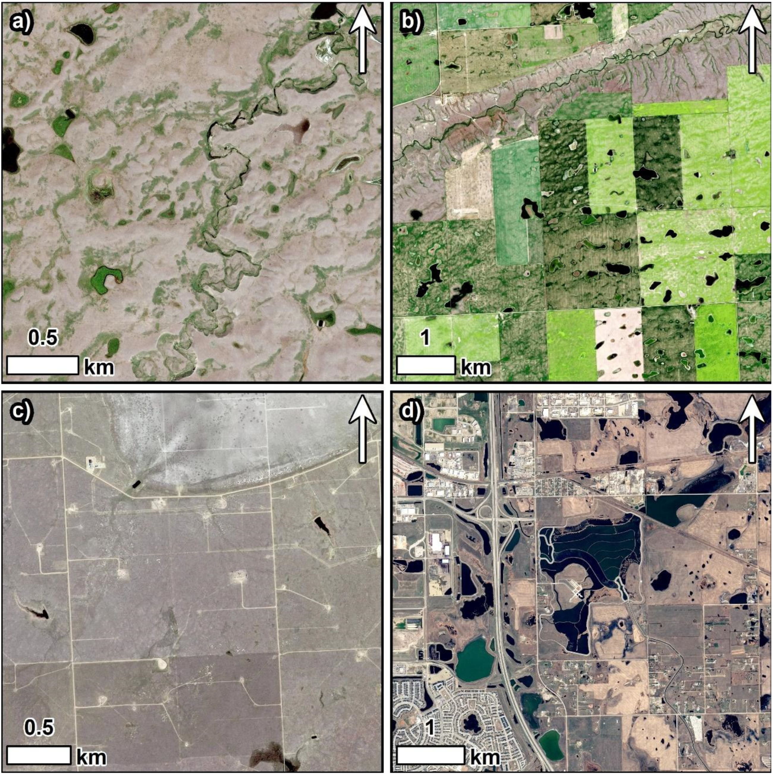
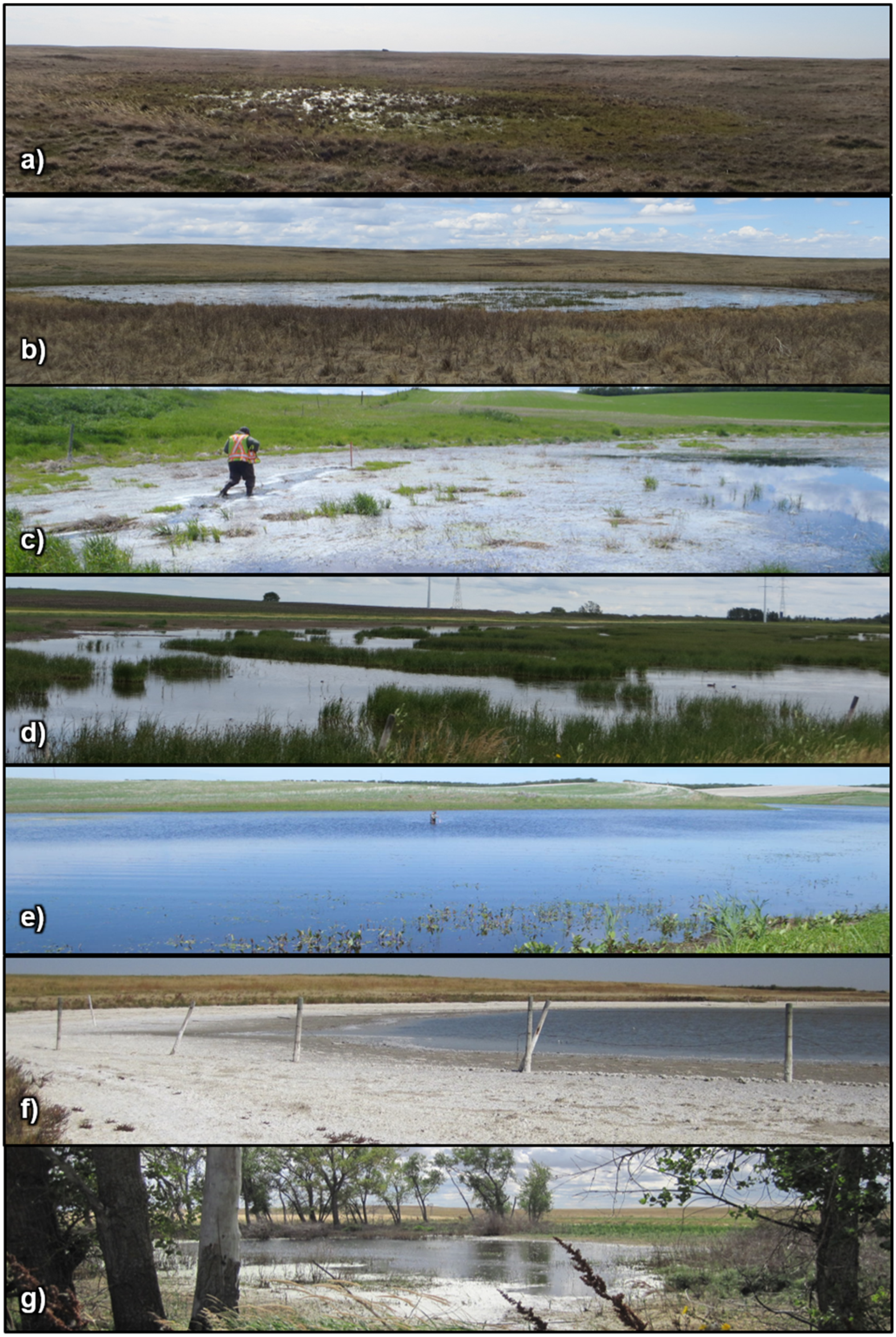
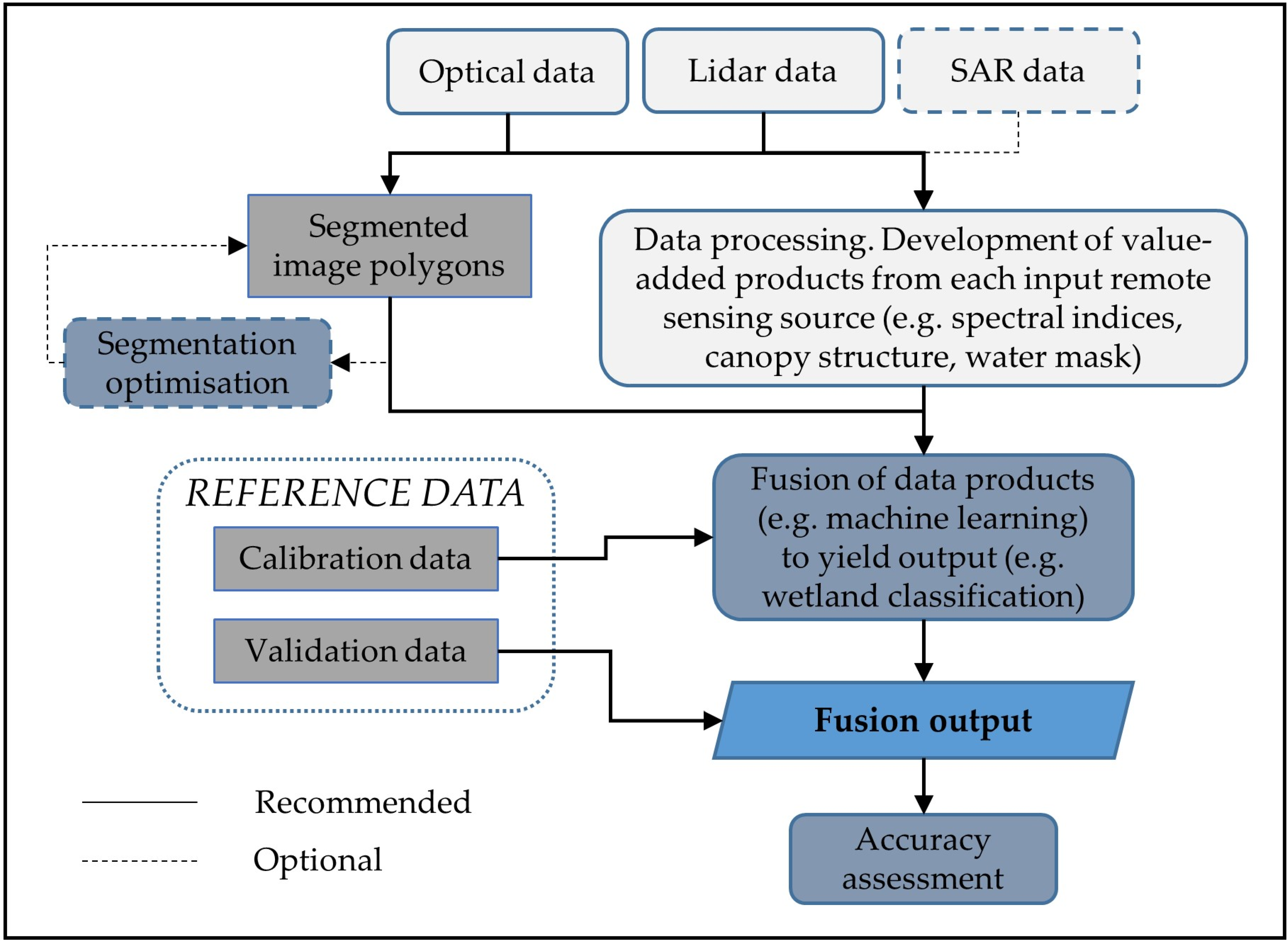
Table 1.
Vegetation community zones and associated wetland hydroperiod definitions for marshes and SOW wetland types according to Stewart and Kantrud.
Table 1.
Vegetation community zones and associated wetland hydroperiod definitions for marshes and SOW wetland types according to Stewart and Kantrud.
| Wetland Type | Hydroperiod | Vegetation Community Zone 1 |
|---|---|---|
| Ephemeral (I) | Surface water is only present for a brief period in early spring. | Wetland low prairie zone |
| Temporary (II) | Surface water is present following a flooding event such as snowmelt or precipitation. | Wet meadow |
| Seasonal (III) | Surface water is present throughout the majority of the growing season but is often dry by summer’s end. | Shallow wetland |
| Semi-permanent (IV) | Surface water is present almost year-round, excluding periods of drought. | Deep wetland |
| Permanent (V) | Surface water persists year-round. | Open water |
| Intermittent (VI) | Alternates between saline open water and exposed bottom. | Alkaline |
1 The plant community zone reflects the plant community found in the deepest portion of a wetland covering more than 25% of the total area in the majority of years and can be used as an indicator of wetland type. Roman numerals are equivalent to wetland class by Stewart and Kantrud [26].
Publisher’s Note: MDPI stays neutral with regard to jurisdictional claims in published maps and institutional affiliations. |
© 2021 by the authors. Licensee MDPI, Basel, Switzerland. This article is an open access article distributed under the terms and conditions of the Creative Commons Attribution (CC BY) license (https://creativecommons.org/licenses/by/4.0/).
Share and Cite
MDPI and ACS Style
Montgomery, J.; Mahoney, C.; Brisco, B.; Boychuk, L.; Cobbaert, D.; Hopkinson, C. Remote Sensing of Wetlands in the Prairie Pothole Region of North America. Remote Sens. 2021, 13, 3878. https://doi.org/10.3390/rs13193878
AMA Style
Montgomery J, Mahoney C, Brisco B, Boychuk L, Cobbaert D, Hopkinson C. Remote Sensing of Wetlands in the Prairie Pothole Region of North America. Remote Sensing. 2021; 13(19):3878. https://doi.org/10.3390/rs13193878
Chicago/Turabian StyleMontgomery, Joshua, Craig Mahoney, Brian Brisco, Lyle Boychuk, Danielle Cobbaert, and Chris Hopkinson. 2021. "Remote Sensing of Wetlands in the Prairie Pothole Region of North America" Remote Sensing 13, no. 19: 3878. https://doi.org/10.3390/rs13193878
Note that from the first issue of 2016, this journal uses article numbers instead of page numbers. See further details here.