
3D Octave and 2D Vanilla Mixed Convolutional Neural Network for Hyperspectral Image Classification with Limited Samples


1
College of Computer Science and Engineering, Zhejiang University of Technology, Hangzhou 310014, China
2
College of Articial Intelligence, Hebei University of Technology, Tianjin 300131, China
*
Author to whom correspondence should be addressed.
Remote Sens. 2021, 13(21), 4407; https://doi.org/10.3390/rs13214407
Submission received: 14 September 2021
/
Revised: 29 October 2021
/
Accepted: 29 October 2021
/
Published: 2 November 2021
(This article belongs to the Section Remote Sensing Image Processing)
Abstract
:Owing to the outstanding feature extraction capability, convolutional neural networks (CNNs) have been widely applied in hyperspectral image (HSI) classification problems and have achieved an impressive performance. However, it is well known that 2D convolution suffers from the absent consideration of spectral information, while 3D convolution requires a huge amount of computational cost. In addition, the cost of labeling and the limitation of computing resources make it urgent to improve the generalization performance of the model with scarcely labeled samples. To relieve these issues, we design an end-to-end 3D octave and 2D vanilla mixed CNN, namely Oct-MCNN-HS, based on the typical 3D-2D mixed CNN (MCNN). It is worth mentioning that two feature fusion operations are deliberately constructed to climb the top of the discriminative features and practical performance. That is, 2D vanilla convolution merges the feature maps generated by 3D octave convolutions along the channel direction, and homology shifting aggregates the information of the pixels locating at the same spatial position. Extensive experiments are conducted on four publicly available HSI datasets to evaluate the effectiveness and robustness of our model, and the results verify the superiority of Oct-MCNN-HS both in efficacy and efficiency.
1. Introduction
Hyperspectral images (HSIs), as an important outcome of remote sensing data recording both abundant spatial information and hundreds of spectrum bands on the earth surface, play a significant role in many fields, such as environmental monitoring [1,2,3], fine agriculture [4], military applications [5], among others. In multitudinous applications, how to deal with information redundancy and extract effective features for precisely distinguishing different targets is a fundamental issue that has drawn increasing attention in recent years.
Considering the rich spectral information in HSIs, several typical machine learning classifiers are used for target discrimination, for example, the k-nearest neighbor (kNN) [6], decision tree [7], extreme learning machine (ELM) [8], support vector machine (SVM) [9], and random forest (RF) [10]. Although these algorithms can construct a feature representation based on the feature similarity among pixels, they perform suboptimally due to the existence of spectral variability in intra-category pixels and spectral similarity in inter-categories pixels. To remedy this redundancy problem, some dimensionality reduction techniques focusing on extracting effective features are widely used, such as principal component analysis (PCA) [11], independent component analysis (ICA) [12], and linear discriminant analysis (LDA) [13]. However, the aforementioned methods merely utilize the properties in the spectral domain but ignore the inherent characteristics along the spatial domain, which may cause misclassified pixels to some extent and lead to the “salt-and-pepper” noise on the classification maps. Thus, in order to further exploit the universal properties, some classification methods have been developed jointly considering spatial-spectral correlation information, for instance, sparse representation [14], Markov random field [15], and edge-preserving filtering [16], to name just a few.
Recently, research on HSI classification is undergoing a paradigm shift. This phenomenon is attributed to the superpower of deep learning-based methods [17,18] on the hierarchical learning ability of high-level abstract features, which has pushed the traditional handcrafted, feature-based models aside. The stacked autoencoder (SAE) [19] and the deep belief network (DBN) [20] pioneer the probing into feature acquisition of HSIs, owing a good deal to their strong nonlinear capabilities. However, due to their compulsive requirement of a one-dimensional input format, a significant amount of effective information would inevitably be discarded while applying these methods into HSI imagery. To alleviate this issue, 1D CNNs [21] for extracting spectral features, 2D CNNs [22,23,24] for acquiring spatial context information, and 3D CNNs [25,26,27] for jointly obtaining spatial–spectral information have been successively proposed, which have promoted convolutional neural networks (CNNs) as the most popular network for HSI processing. Specifically, both 1D convolution and 2D convolution lack consideration of certain feature correlations to some extent, while 3D convolution captures spatial–spectral priors at the expense of a huge computational cost. For the purpose of extracting the most universal features, different kinds of fusion strategies have been derived for a better discriminative ability. Typically, in [28,29], a parallel dual-branch framework is proposed, where 1D convolution is used to extract spectral features and a 2D CNN is added for spatial information acquisition. Moreover, in our previous work [30], by attaching one 2D convolution layer after three 3D convolution layers, we accomplish the spatial–spectral feature integration by simply fusing the generated feature maps, and meanwhile implicitly realize a dimensionality reduction for better efficiency.
With the unceasing intensifying of the comprehension of traditional convolution operations, some fantastic convolution methods have recently been proposed and exhibit appealing performance. For instance, in [31], conditionally parameterized convolution is proposed to break through the setting of sharing convolution kernels for all of the examples in the vanilla convolution operation and learn specialized convolutional kernels for each sample. Reference [32] proposes a network that extracts vital information by performing relatively complex operations on the representative part disassembled from the input feature maps, and extracts hidden information by using lightweight operations on the remaining part, thereby improving the accuracy with acceptable reasoning speed. In addition, some novel architectures have also been considered for further performance improvement. For instance, the graph convolution networks (GCNs) [33,34] could introduce a local graph structure to promote the convolution characteristics. However, how to transform the data into a graph structure and reveal the deep relationship between nodes is still challenging. Besides, recurrent neural networks (RNNs) [35,36,37] regard all of the spectral bands as an image sequence whose drawback lies in the short consideration of spatial features. Moreover, the high computational cost and disappointing performance under limited samples are significant bottlenecks of GCNs and RNNs in the HSI classification task, particularly when using large-scale image data. Therefore, considering only a laptop computer as a supporting device, convolution operations are still the core technology to jointly harvest spatial–spectral information.
In addition to constructing different convolution methods for better feature extraction, several other strategies have also been proposed to improve the effectiveness of information acquisition. Two representatives are the attention mechanism [38,39,40] emphasizing key points while suppressing interference, and the covariance pooling operation for characteristic information sublimation. On the one hand, the attention mechanism pursues highlighting the spectral bands and spatial locations that have more obvious discriminative properties while suppressing the unnecessary ones, thereby the representation ability of CNNs can be greatly enhanced. In [30], motivated by the channel-wise attention mechanism, a scheme of a channel-wise shift is proposed to highlight the important principal components and recalibrate the channel-wise feature response. On the other hand, the covariance pooling operation [22,30,41] attempts to obtain second-order statistics by calculating the covariance matrix between feature maps, which leads to a more significant and compact representation. However, in the process of mapping a covariance matrix on the Riemannian manifold space to the Euclidean space, the loss of partial effective information and the addition of several extra calculation operations turn into the evident disadvantages of the covariance pooling scheme.
To overcome the aforementioned drawbacks and capture more detailed spatial–spectral information, this paper proposes an improved CNN-based network architecture for the HSI classification problem. Specifically, based on the most recently proposed MCNN-CP [30] model (3D-2D mixed CNN with covariance pooling), our model further employs 3D octave and 2D vanilla mixed convolutions with homology shifting. The model is referred to as Oct-MCNN-HS for short. Through a comprehensive comparison with the other state-of-the-art methods, Oct-MCNN-HS achieves twofold breakthroughs both in convergence speed and classification accuracy in the classification task with small-size labeled samples. The main contributions of our work are listed as follows.
- Aiming at the classification of tensor-type hyperspectral images, we design 3D octave and 2D vanilla mixed convolutions in order to mine potential spatial–spectral features. Specifically, we first decompose the feature maps into different frequency components, and then apply 3D convolutions to accomplish the complementation of inter-frequency characteristics. Finally, the 2D vanilla convolution is attached to fuse along the channel direction of the feature maps, which reduces the output dimension and improves the generalization performance.
- Note that the final feature maps are sent to the classifier along the channel dimension, that is, the information at the same spatial location is discretely distributed in the vector form. Therefore, we propose the homology-shifting operation to aggregate the information of the same spatial location along the channel direction to ensure more compact features. It is commendable that homology shifting can enhance the generalization performance and stability of the model without any computational consumption.
- Extensive experiments are conducted on four HSI benchmark datasets with small-sized labeling samples. The results show that the proposed Oct-MCNN-HS model outperforms other state-of-the-art deep learning-based approaches in terms of both efficacy and efficiency. The proposed model with optimized parameters has been uploaded online at https://github.com/, accessed on ZhengJianwei2/Oct-MCNN-HS, whose source code will be coming soon after the review phase.
The remainder of this paper is organized as follows. Section 2 gives a brief review of the related works. In Section 3, we present the proposed network architectures in detail. The comprehensive experiments on four HSIs are conducted in Section 4. Finally, Section 5 draws the conclusion and provides some suggestions for future work.
2. Related Work
Based on MCNN-CP [30], the backbone architecture of our model is formed by trimming the suboptimal parts and retaining the competitively capable ones. In this subsection, we roughly review the reserved components for self-containment. Based on the fact that HSIs are naturally with a tensor structure and contain redundant spectral information, MCNN-CP starts with a dimensionality reduction operation using PCA, followed by 3D-2D mixed convolution layers obtaining representative features. Afterward, the covariance pooling scheme is appended to fully extract the second-order information from feature maps. In addition, in [42], the 2D octave convolution based on multi-frequency feature mining was proposed, showing its superiority.
2.1. 3D-2D Mixed Convolutions
By virtue of its dramatic performance, convolution treatment is the most favorable modus operandi in the visual processing community since the birth of deep learning. Practically, 2D convolution and 3D convolution are the two most representative. Among these two, 2D convolution seeks mainly for spatial features but neglects the appreciatory inter-spectral information, making it insufficient to fully acquire discriminative features and perform suboptimally for most applications. Relatively speaking, 3D convolution can naturally extract more discriminative spatial–spectral information due to the tensor essence of hyperspectral images. The most unacceptable point associated with 3D convolution is, as the scale of generated feature maps increases, the operation gets much more complicated and huge computational demand is required. Therefore, probing a balanced way to integrate the advantages of 3D convolutions capturing more information and 2D convolution running with higher efficiency is a worthwhile attempt. In our studies, we found a significantly effective yet easy-to-accomplish way for this purpose is simply adding a layer of 2D convolution after several 3D convolutional operations. To be specific, the added 2D convolution can fuse the feature maps generated by the 3D convolutions, thereby playing a dual role of obtaining richer information while simultaneously reducing the dimension of the spectral bands.
2.2. Covariance Pooling
The covariance pooling method computes the covariance matrix between different feature maps, and realizes the mapping from the Riemannian manifold space to the Euclidean space through the logarithmic function, so as to obtain a vector with second-order information for classification. To some extent, as a plug-and-play method, covariance pooling can be regarded as an operation to sublimate the information of the feature maps generated by convolutions.
However, the covariance pooling method also has some unavoidable shortcomings. Firstly, non-trivial covariance computation will inevitably require additional calculation and storage consumption. Secondly, due to the need for space mapping, there must be some loss of effective information to a certain extent. Therefore, it is necessary to hunt for a simpler feature information sublimation operation that can further supply the model more formidable mining capabilities.
2.3. 2D Octave Convolution
In [42], the authors claim that the output feature maps of the convolution layer are characteristically similar to that of the natural image, which may prompt a factorization of a high spatial frequency locally describing the fine details and another low spatial frequency representing the global structure. Consequently, 2D octave convolution is proposed to process the two components with different 2D vanilla convolutions (ordinary convolutions without additional operations) at their corresponding frequency and obtain global and local information under two resolution representations. Since the two frequency components are decomposed along the channels, the total number of feature maps remains constant, while the resolution of the low-frequency part is reduced. This reduces the spatial redundancy for inference acceleration and enlarges the receptive field for rich contextual information. However, this method incurs new hyperparameters, which cannot be empirically set and requires an exhausting searching process.
3. Methodology
In this section, as shown in Figure 1, we introduce our proposed Oct-MCNN-HS. Following a similar backbone architecture as MCNN-CP, we also preprocess the HSI data using the PCA technique, and adopt the patch-wise treatment to the data as the input. Different from MCNN-CP, we first develop 3D octave convolutions to jointly extract the spectral–spatial information hidden in the principal components. By considering the benefits of different frequency components, 3D octave convolutions disassemble the feature maps into two parts, i.e., high-frequency components and low-frequency components, through which the generated dual-branch and multi-scale convolutions can provide even more discriminative features. Afterward, the homology-shifting operation is imposed on our model to aggregate the pixel information at the same spatial position along the spectral dimension, thereby further pursuing the sublimation of the feature information.
3.1. 3D Octave and 2D Vanilla Mixed Convolutions
Although the 3D-2D mixed convolutions perform well in spatial–spectral feature extraction, it neglects the truth that most visual information can be conveyed at different frequencies. Following the fact that HSIs can be decomposed into low spatial frequency components describing a smooth structure and high spatial frequency components with fine details, we decompose the output features of the convolutional layers into features with different spatial frequencies. As shown in Figure 1, we construct 3D octave convolutions to replace 3D vanilla convolution layers, which manifests a multi-frequency feature representation. Roughly speaking, the convolutional feature maps are up-sampled and down-sampled to obtain new maps with different spatial resolutions. Evidently, the low spatial resolution maps are employed as low-frequency components, and the high-resolution maps are introduced as high-frequency components.
Let denote the input tensor, as a whole, we regard it as a high-frequency module that can be disassembled into multi-frequency components through two-branch and multi-scale convolutions. One branch performs a 3D vanilla convolution to seek high-frequency component , and the other branch executes both average pooling and 3D vanilla convolution to recruit low-frequency component . Note that the original Oct-Conv [42] explicitly factorizes X along a channel-wise dimension into and , where is the proportion of channels allocated to the low-frequency part. Different from this, we apply the abovementioned two-branch and multi-scale approach to fully capture the predominant information and avoid an exhausting search for the optimal hyperparameter . The specific formulations are as follows:
where denotes the 3D convolution, and represent the intra-frequency and inter-frequency convolution kernels, respectively, and is an average pooling operation with kernel size and stride s.
Obtaining from input X can be seen as a simplified octave convolution, where the paths related to the low-frequency input are disabled and only two paths are adopted. In contrast, as shown in Figure 1, the module from to is a complete octave convolution with a four-branch structure, which effectively extracts the information of different frequency components in their corresponding frequency tensor and synchronously fulfills inter-frequency communication. Specifically for high-frequency component , we first calibrate the impact of high-frequency component by using a regular 3D convolution for the intra-frequency update, and then up-sample the feature maps generated by convolving a low-frequency component to achieve inter-frequency communication. Similarly, the low-frequency component is employed when seeking intra-frequency update and the high-frequency component is down-sampled for inter-frequency communication, thereby jointly obtaining the low-frequency feature maps . Thus, the equations of and can be formulated as
where and denote the intra-frequency update, while and imply inter-frequency communication, and is an up-sampling operation by a factor of s via the nearest interpolation.
Finally, considering the repercussions of spatial resolution on subsequent operations, similar to the generation and calculation of , we obtain the low-frequency output Y by jointly performing 3D convolutions on low-frequency and feature maps obtained by down-sampling the high-frequency . The formulation of Y is
In a nutshell, although 3D octave convolutions slightly lead to increased consumption, they provide more discriminative features by decomposing the feature maps into different frequency components, and also accomplish the complementation of spatial features through two mechanisms, viz., intra-frequency update and inter-frequency communication. In other words, this multi-scale and dual-branch structure deserves to be introduced for more information extraction. After that, a layer of 2D vanilla convolutional layer is attached to pursue the fusion of feature maps along the channel direction, by which the output Z can be obtained achieving both a dimensionality reduction and information aggregation. The formulation of Z is
where denotes the 2D vanilla convolution. By constructing a hybrid of 3D Octave and 2D vanilla convolution, it is not only possible to effectively mine the potential spatial–spectral information from the tensor-type hyperspectral data, but also to achieve a balance between convergence performance and discrimination efficiency. In this way, the generalization performance of the designed model on a different dataset is improved to a certain extent.
3.2. Homology Shifting
During our previous studies, we found that utilizing a certain specific sublimation operation before sending the generated feature maps to the classifier has the potential for revealing deeper information. For example, in [30], the covariance pooling scheme can obtain second-order statistics by calculating the covariance between spatial–spectral feature maps, thereby significantly improving the classification accuracy when limited training samples are available. In this work, we attempt to explore the homology-shifting operation for further feature excavation without any extra demand of computational cost.
Essentially, the homology-shifting operation can be regarded as an image reshaping operation, as shown in Figure 2, which only needs to aggregate the pixel information at the same spatial position along the channel dimension and requires no extra computational overhead. Specifically, the homology-shifting operation can be formulated as
where is the feature maps following convolution operations, is the abbreviation of the homology-shifting operation, is composed of the corresponding pixels at the ith spatial position on X, is the block generated by regrouping along the channel direction, represents the final output feature map, and the function indicates that blocks are spliced according to the original spatial position.
By sequentially shifting the feature maps of spatial size, each block corresponding to the ith spatial position on the feature maps are reorganized along the channel direction to form block . Consequently, blocks are spliced together and an aggregated feature map is generated. After continuously extracting features through convolutions, the feature maps generated by consistently down-sampling treatment in space can already ensure of the obtained information being useful for a certain high-level semantic. On that basis, performing the additional homology-shifting operation would further merge the spatial–spectral information on multiple feature maps into a more discriminative one. Finally, the transformed feature map is flattened into a vector and input into the classifier; to a certain extent, the information of different spectral bands and the same spatial location can be aggregated.
Compared with the covariance pooling scheme, homology shifting has several significant advantages. On one hand, covariance pooling requires the computation of a covariance matrix between different feature maps. Moreover, this should be further fed into a spatial mapping step for the final discriminant vector. In contrast, the construction of homology shifting only goes through a simple pixel reorganization following the original convolution operation, which does not cost any additional computational overhead. On the other hand, when covariance pooling is applied, certain information loss inevitably happens during the mapping from Riemannian manifold space to Euclidean space. This phenomenon would not occur under the homology-shifting process, in which case all of the elements of convolution-generated feature maps are fully kept. Instead, more information utilization would be earned owing to the shifting mechanism. These merits guarantee an open prospect for the application of homology shifting in discriminative feature extraction.
4. Experiments
In this section, we specify the hyperparameters for the model configuration and evaluate the proposed methods using three classification metrics, including overall accuracy (OA), average accuracy (AA), and kappa coefficient (Kappa). For assessing the classification performance of the Oct-MCNN-HS framework, we introduce four publicly available HSI datasets, including Indian Pines (IP), the University of Houston (UH), the University of Pavia (UP), and Salinas Scene (SA). In all of the experimental scenarios, we repeatedly run all of the algorithms five times with randomly selected training data and report the average results of the main classification metrics to reduce the influence of random initialization.
4.1. Data Description
The four used datasets are illustratively shown in Table 1, Table 2, Table 3 and Table 4. In addition, a more detailed description of each dataset is given as follows.
- (1)
- Indian Pines (IP): The first dataset was captured in 1992 by the AVIRIS sensor over an agricultural area in northwestern Indiana. The image includes pixels and 200 spectral bands (24 channels are eliminated owing to noise) in the wavelength range of 0.4 to 2.5 m. In this scene, there are 16 representative land-cover categories to be classified.
- (2)
- University of Houston (UH): The second dataset was gathered in 2017 by the NCALM instrument over the University of Houston campus and its neighborhood, comprising 50 spectral channels with a spectral coverage ranging from 0.38 to 1.05 m. With pixels, this dataset is composed of 20 representative urban land-cover/land-use types.
- (3)
- University of Pavia (UP): The third dataset was collected in 2002 by the ROSIS sensor from northern Italy. The image contains spatial resolution and 103 (12 bands are removed due to the noise) bands with a spectral coverage ranging from 0.43 to 0.86 m. Approximately 42,776 labeled samples with 9 classes are extracted from the ground-truth image.
- (4)
- Salinas Scene (SA): The fourth dataset was acquired by the AVIRIS sensor over the Salinas Valley, California, containing 204 spectral bands (20 water absorption bands are discarded) and pixels with the spatial resolution of 3.7 m. The image is divided into 16 ground-truth classes with a total of 54,129 labeled pixels.
4.2. Framework Setting
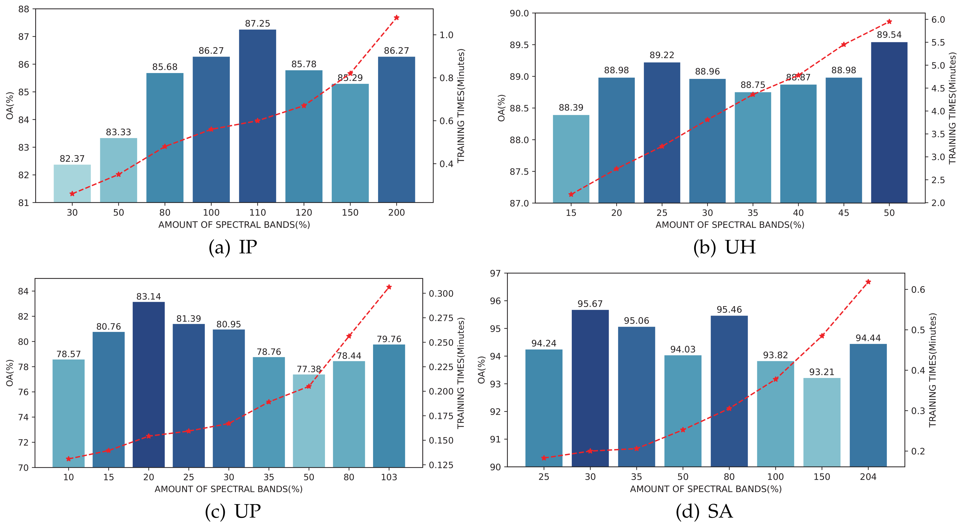
Since the designed Oct-MCNN-HS model exploits the PCA to achieve a balance between redundant information removal and effective feature retention, the number of preserved components is an indispensable hyperparameter for the classification of a new HSI. In practice, when sufficient samples are available, the number of principal components is less sensitive for the classification results. However, in this work, we focus more on the classification performance in the case with limited samples. In our experiments, for different HSI data, different selections of the component number are tested to generate the classification results. The specific values are shown in the horizontal axis of Figure 3. Since the practical component number would have a significant impact on both the classification accuracy and running efficiency, we list both the OA value and the training duration. From this figure, our first observation is that the peak performance varies along with different HSIs as well as the number of retained components. Overall, following this figure and taking a balanced consideration of the accuracy and training duration, we finally set 110, 25, 20, and 30 as the final values for the IP, UH, UP, and SA datasets, respectively.
4.3. Experimental Setup
To demonstrate the appealing performance of our model, we compare Oct-MCNN-HS with several recently published and deep learning-based HSI classification methods, including HybridSN [43], SSRN [26], A-SPN [41], and MCNN-CP [30]. It is worth mentioning that, except for the missed evaluation on the UH dataset, MCNN-CP has demonstrated state-of-the-art classification performance whenever under large or small sample sizes on the IP, UP, and SA datasets. Moreover, we will find from our experimental results that, on the basis of MCNN-CP, the newly proposed Oct-MCNN-HS can move a remarkable breakthrough forward in performance. Four numerical metrics are used to record the quantitative results from each competing model, including class-wise accuracy, OA, AA, and Kappa. In addition to the classification performance comparison in the case of limited samples, for further investigating the superiority of our model in various scenarios, we also exploit different training sizes for the experiments. It is worth noting that the number of instances of different classes may vary greatly, which results in the well-known class imbalance issue. To fairly balance the accuracies of the minority and the majority classes, we set the “class_weight” attribute in the Keras framework to “auto” following the similar idea that was intensively discussed in [44]. Specifically, as shown in Figure 1, a class weight would be optionally assigned to each class striving for an equal contribution of each one to the loss function. For the datasets IP and UH, certain occasions that quite limited the sample sizes would occur when an extremely low sample ratio, e.g., 1% or 0.5%, is adopted. For example, when one uses 1% samples as the training/validation set, then the 7th and 9th classes of IP data both consist of zero samples. Accordingly, the class weight cannot be correctly derived and the mechanism is insufficient to tackle the imbalance issue. Therefore, we borrow the sampling scheme used in EPF [16] to earn a more balanced performance. In the implementation, a fixed number of training samples for each category is initially set. For certain categories having smaller samples than the given number, half of the samples are used for training, and the remaining vacancy is filled up by the ones from other rich categories.
For all of the hybrid models combining 3D and 2D convolutions, to circumvent the explosion of the parameter amount and ensure their performability on the commonly equipped laptop, we set three 3D convolution layers with size (8 volumes of size), , and convolution kernels, respectively, to extract sufficient features and one 2D convolution operation with size (64 volumes of size) kernel to fuse the feature maps. It is worth noting that to ensure a full information discovery, we perform the operation of padding-with-zeros for all of the 3D convolutions. In addition, different from the MCNN-based models, is set as the kernel size of the 2D convolution layer in all of the Oct-MCNN-based models. A detailed summary of the proposed architecture in terms of the layer types, output map shapes, and the number of parameters is given in Table 5.
In all of the experiments, the patch size, the dropout proportions of the fully connected layers, the training epoch, the batch size, the optimization algorithm, and the learning rate are set to , , 100, 256, adam, and , respectively. The experiments are conducted on a personal laptop equipped with an Intel Core i7-9750H processor of GHz, 32 GB of DDR4 RAM, and NVIDIA GeForce GTX 1650 GPU. The coding is carried out under the TensorFlow framework with the programming language Python . In the meantime, we configure the environment with CUDA and cuDNN for GPU acceleration.
4.4. Performance Comparison
The first comparison experiments are conducted using limited samples. Specifically, considering the imbalance problem of the training samples of the IP and UH datasets, 5 samples per category (a total of 80 samples) and approximately 100 samples per class (2000 in total) are respectively adopted as the training set for model optimization. For the other two datasets, i.e., UP and SA, of each labeled cube is selected for training groups and verification groups, respectively, and the remaining of the samples are used for performance evaluation. The generated results of our proposed model, as well as several representative models, i.e., HybridSN [43], SSRN [26], A-SPN [41], and MCNN-CP [30], are shown in Table 6, Table 7, Table 8 and Table 9. From these tables, one can easily observe that the method of HybridSN performs relatively poorer than the others. Although A-SPN achieves favorable results on the IP dataset, it performs poorer than MCNN-CP on the other three datasets, i.e., UH, UP, and SA. Note that MCNN-CP has proved its remarkable capability of discriminative feature extraction on IP, UP, and SA [30]. Yet encouragingly, Oct-MCNN-HS developed in this paper consistently achieves better classification results, which demonstrates its superiority in extracting formidable features compared with MCNN-CP. Evidently, among all of the compared models, Oct-MCNN-HS achieves the optimal classification performance and also with lower standard deviation, which demonstrates the advantage of mixed convolutions and homology shifting.
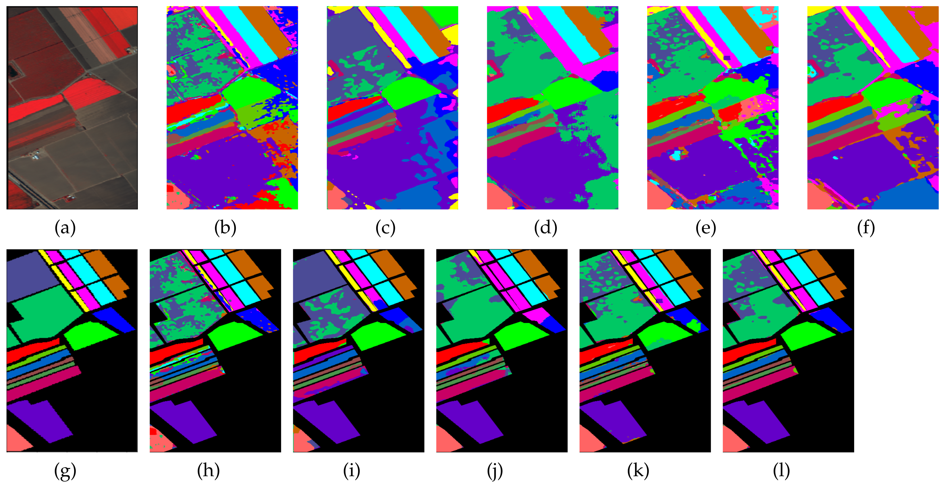
Together with the false-color images of the original HSI and their corresponding ground-truth maps, Figure 4, Figure 5, Figure 6 and Figure 7 further visualize the classification results on the four datasets. From these figures, one can see that the qualitative comparison evidently confirms the quantitative comparison shown in Table 6, Table 7, Table 8 and Table 9. Concretely, the classification maps generated by HybridSN are full of noisy points and the other methods achieve better results with clearer contours and sharper edges. However, due to the limitation of training size, there are still some scattered points that unavoidably exist in some categories. Again, by carefully comparing these maps with the ground-truth ones, we argue that the maps learned from Oct-MCNN-HS hold the highest fidelity compared to the others. All the remaining competitors generate more artifacts, e.g., broken lines, blurry regions, and scattered points, to some extent.
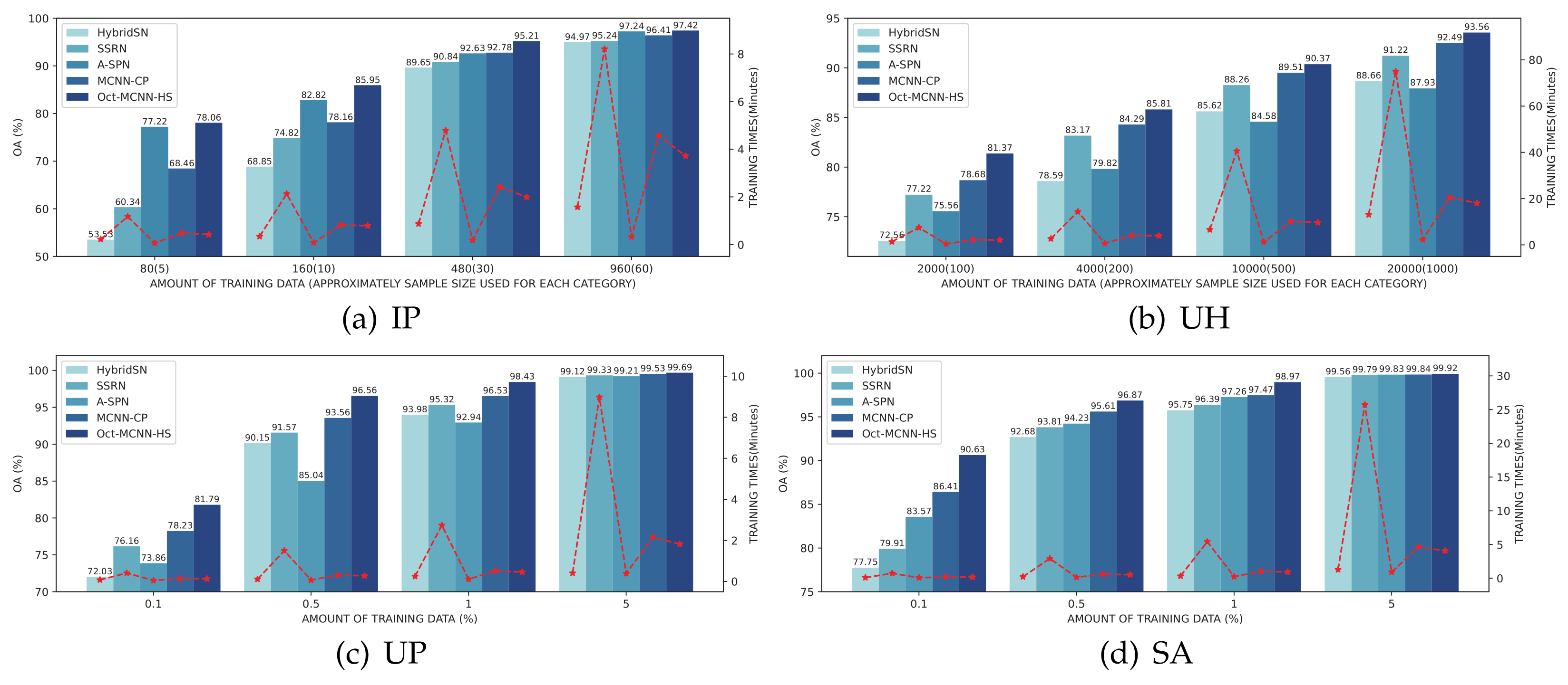
For the sake of verifying the effectiveness of our model under various training samples, in the third experiment, we evaluate the competing approaches using sample proportions traversed from the candidate set {80, 160, 480, 960} for IP, {2000, 4000, 10,000, 20,000} for the UH, and {0.1%, 0.5%, 1%, 5%} for the UP and SA, respectively. In Figure 8, the overall accuracies and training time of different classifiers are illustrated. Our first observation is that Oct-MCNN-HS always ranks in the top place in all of the cases. Although the gap gradually shrinks along with the increasing size of the training samples, the gains of our method over the other competitors are quite significant when limited samples are available. The phenomenon is reasonable since all of the candidate methods perform well with sufficient samples. Overall, the practical performance can be arranged in descending order as Oct-MCNN-HS > MCNN-CP > A-SPN > SSRN > HybridSN. Note that, taking only the accuracy into account, the performance of A-SPN fluctuates more strongly on different datasets than others. In terms of running efficiency, we can also conclude from this figure that in all of the cases, the convergence speed of our Oct-MCNN-HS is significantly ahead of SSRN and MCNN-CP. Although our method lags behind HybridSN and A-SPN due to the requirement of more retained components in the PCA step, the speed gap between them lies in an acceptable range. The efficiency together with the accuracy verifies that our proposed method enjoys a high robustness, favorable generalization, and excellent convergence under different scenarios.
To dig deeply into the behaviors of 3D octave and 2D vanilla mixed convolutions in our network model, several variants that use 3D-2D mixed convolutions (MCNN) as the backbone are further introduced as the competitors. Furthermore, the advantage of homology shifting over covariance pooling on the role of feature sublimation should also be explored. A total of seven deep learning-based approaches are used in this experiment, including the original MCNN, MCNN plus covariance pooling (MCNN-CP), MCNN plus homology shifting (MCNN-HS), 3D octave CNN, MCNN using 3D octave convolution (Oct-MCNN), Oct-MCNN plus covariance pooling (Oct-MCNN-CP), and Oct-MCNN-HS. In the implementation, 160 and 4000 samples for the IP and UH datasets, and 0.5% training samples for the UP and SA are used for model optimization. The classification results are shown in Figure 9.
Taking MCNN as the baseline, the first observation is that the two techniques presented, i.e., octave convolution and homology shifting, both benefit the model. However, the improvement from the covariance pooling scheme cannot be guaranteed. For Oct-MCNN-CP, it even underperforms the counterpart, i.e., Oct-MCNN, in all four cases. With homology shifting involved, both MCNN-HS and Oct-MCNN-HS outperform their counterparts, evidently. Comparing three naive models, i.e., MCNN, 3D Octave CNN, and Oct-MCNN, 3D octave convolution enjoys better feature extraction capabilities. Moreover, attaching a layer of 2D vanilla convolution after 3D octave convolutions to form the Oct-MCNN model can further ensure better performance. In our studies, we can assure that the addition of homology shifting would incur gains both in efficacy and efficiency. With both of these two techniques involved, the final Oct-MCNN-HS outperforms all of the competitors in all of the experiments. In terms of classification accuracy, all of these variants can be sorted in a descending sequence as Oct-MCNN-HS>Oct-MCNN>MCNN-HS>MCNN.
4.5. Discussion
Specific to the roles of mixed convolutions and feature sublimation, several conclusions can also be drawn. First of all, experiments on the MCNN- or Oct-MCNN-based models prove that compared with covariance pooling scheme, homology-shifting operation has more information involved, leading to better effectiveness on a variety of datasets. In addition, 3D octave convolutions provide more multi-scale supplementary information through feature maps of different resolutions, which will positively manifest the relationship between feature maps, especially the difference between low-frequency maps and high-frequency maps. What is more, by attaching a layer of 2D vanilla convolution after 3D octave convolutions, the feature maps can be further merged along channels, thereby reducing the dimensionality and aggregation information. On that basis, covariance pooling obtains the second-order statistics by calculating the covariance matrix between the feature maps. This cannot be positively paired with the Oct-MCNN model. Relatively, homology shifting as a pixel reorganization operation concentrates the information of pixels in the same location along the channel direction, pushing more features to be aggregated. Although the combination of it and the non-trivial Oct-MCNN model cannot achieve a significant speed-up in the training process, it improves the classification accuracy without incurring any extra computation consumption.
5. Conclusions
In this work, a new network architecture for HSI classification, namely Oct-MCNN-HS, is proposed involving 3D octave and 2D vanilla mixed convolutions. Specifically, we first adopt a principal component analysis to reduce the dimension and redundancy of spectral bands. In the feature extraction stage, we construct dual-branch and multi-scale 3D octave convolutions through up- and down- sampling strategies, as well as intra-frequency update and inter-frequency communication mechanisms to obtain more discriminative information. Subsequently, a layer of 2D vanilla convolution is attached to fuse the feature maps generated by 3D octave convolutions along the channel direction, thereby reducing the dimensionality and aggregate information. In addition, for the sake of better feature sublimation, the homology-shifting operation is employed to assemble the pixels information located in the same spatial position along with different maps. The final model, Oct-MCNN-HS, constructed with the above two information aggregation operations, i.e., 2D vanilla convolution and homology shifting, achieves breakthroughs both in the convergence speed and classification accuracy on several open available HSIs with scarce labeled samples. In the near future, we will focus on automatic search mechanisms to get rid of the trouble tuning of hyperparameter selection.
Author Contributions
Conceptualization, Y.F. and J.Z. (Jianwei Zheng); methodology, Y.F. and J.Z. (Jianwei Zheng); validation, Y.F.; formal analysis, Y.F., J.Z. (Jianwei Zheng), and M.Q.; writing—original draft preparation, Y.F., J.Z. (Jianwei Zheng), and M.Q.; writing—review and editing, Y.F., J.Z. (Jianwei Zheng), C.B., and J.Z. (Jinglin Zhang); funding acquisition, J.Z. (Jianwei Zheng), C.B., and J.Z. (Jinglin Zhang). All authors have read and agreed to the published version of the manuscript.
Funding
This research was funded by the National Key Research and Development Program of China (No. 2018YFE0126100), the Natural Science Foundation of China under Grant Nos. 41775008 and 61602413, the Zhejiang Provincial Natural Science Foundation of China under Grant No. LY19F030016 and LR21F020002, and the Open Research Projects of Zhejiang Lab 2019KD0AD01/007.
Institutional Review Board Statement
Not applicable.
Informed Consent Statement
Not applicable.
Data Availability Statement
Not applicable.
Conflicts of Interest
The authors declare no conflict of interest.
References
- Kuras, A.; Brell, M.; Rizzi, J.; Burud, I. Hyperspectral and Lidar Data Applied to the Urban Land Cover Machine Learning and Neural-Network-Based Classification: A Review. Remote Sens. 2021, 13, 3393. [Google Scholar] [CrossRef]
- Scafutto, R.D.M.; de Souza Filho, C.R.; de Oliveira, W.J. Hyperspectral remote sensing detection of petroleum hydrocarbons in mixtures with mineral substrates: Implications for onshore exploration and monitoring. ISPRS J. Photogramm. Remote Sens. 2017, 128, 146–157. [Google Scholar] [CrossRef]
- Bai, C.; Zhang, M.; Zhang, J.; Zheng, J.; Chen, S. LSCIDMR: Large-scale Satellite Cloud Image Database for Meteorological Research. IEEE Trans. Cybern. 2021, 1–13. [Google Scholar] [CrossRef]
- Pandey, P.; Payn, K.G.; Lu, Y.; Heine, A.J.; Walker, T.D.; Acosta, J.J.; Young, S. Hyperspectral Imaging Combined with Machine Learning for the Detection of Fusiform Rust Disease Incidence in Loblolly Pine Seedlings. Remote Sens. 2021, 13, 3595. [Google Scholar] [CrossRef]
- Makki, I.; Younes, R.; Francis, C.; Bianchi, T.; Zucchetti, M. A survey of landmine detection using hyperspectral imaging. ISPRS J. Photogramm. Remote Sens. 2017, 124, 40–53. [Google Scholar] [CrossRef]
- Ma, L.; Crawford, M.M.; Tian, J. Local Manifold Learning-Based k -Nearest-Neighbor for Hyperspectral Image Classification. IEEE Trans. Geosci. Remote Sens. 2010, 48, 4099–4109. [Google Scholar] [CrossRef]
- Delalieux, S.; Somers, B.; Haest, B.; Spanhove, T.; Vanden Borre, J.; Mücher, C. Heathland conservation status mapping through integration of hyperspectral mixture analysis and decision tree classifiers. Remote Sens. Environ. 2012, 126, 222–231. [Google Scholar] [CrossRef]
- Yu, X.; Feng, Y.; Gao, Y.; Jia, Y.; Mei, S. Dual-Weighted Kernel Extreme Learning Machine for Hyperspectral Imagery Classification. Remote Sens. 2021, 13, 508. [Google Scholar] [CrossRef]
- Melgani, F.; Bruzzone, L. Classification of hyperspectral remote sensing images with support vector machines. IEEE Trans. Geosci. Remote Sens. 2004, 42, 1778–1790. [Google Scholar] [CrossRef] [Green Version]
- Zhang, Y.; Cao, G.; Li, X.; Wang, B.; Fu, P. Active Semi-Supervised Random Forest for Hyperspectral Image Classification. Remote Sens. 2019, 11, 2974. [Google Scholar] [CrossRef] [Green Version]
- Han, Y.; Shi, X.; Yang, S.; Zhang, Y.; Hong, Z.; Zhou, R. Hyperspectral Sea Ice Image Classification Based on the Spectral-Spatial-Joint Feature with the PCA Network. Remote Sens. 2021, 13, 2253. [Google Scholar] [CrossRef]
- Wang, J.; Chang, C.I. Independent component analysis-based dimensionality reduction with applications in hyperspectral image analysis. IEEE Trans. Geosci. Remote Sens. 2006, 44, 1586–1600. [Google Scholar] [CrossRef]
- Chen, M.; Wang, Q.; Li, X. Discriminant Analysis with Graph Learning for Hyperspectral Image Classification. Remote Sens. 2018, 10, 836. [Google Scholar] [CrossRef] [Green Version]
- Cui, B.; Cui, J.; Lu, Y.; Guo, N.; Gong, M. A Sparse Representation-Based Sample Pseudo-Labeling Method for Hyperspectral Image Classification. Remote Sens. 2020, 12, 664. [Google Scholar] [CrossRef] [Green Version]
- Cao, X.; Xu, Z.; Meng, D. Spectral-Spatial Hyperspectral Image Classification via Robust Low-Rank Feature Extraction and Markov Random Field. Remote Sens. 2019, 11, 1565. [Google Scholar] [CrossRef] [Green Version]
- Kang, X.; Li, S.; Benediktsson, J.A. Spectral-Spatial Hyperspectral Image Classification With Edge-Preserving Filtering. IEEE Trans. Geosci. Remote Sens. 2014, 52, 2666–2677. [Google Scholar] [CrossRef]
- Paoletti, M.; Haut, J.; Plaza, J.; Plaza, A. Deep learning classifiers for hyperspectral imaging: A review. ISPRS J. Photogramm. Remote Sens. 2019, 158, 279–317. [Google Scholar] [CrossRef]
- Li, S.; Song, W.; Fang, L.; Chen, Y.; Ghamisi, P.; Benediktsson, J.A. Deep Learning for Hyperspectral Image Classification: An Overview. IEEE Trans. Geosci. Remote Sens. 2019, 57, 6690–6709. [Google Scholar] [CrossRef] [Green Version]
- Madani, H.; McIsaac, K. Distance Transform-Based Spectral-Spatial Feature Vector for Hyperspectral Image Classification with Stacked Autoencoder. Remote Sens. 2021, 13, 1732. [Google Scholar] [CrossRef]
- Li, T.; Zhang, J.; Zhang, Y. Classification of hyperspectral image based on deep belief networks. In Proceedings of the 2014 IEEE International Conference on Image Processing (ICIP), Paris, France, 27–30 October 2014; pp. 5132–5136. [Google Scholar] [CrossRef]
- Chen, Y.; Jiang, H.; Li, C.; Jia, X.; Ghamisi, P. Deep Feature Extraction and Classification of Hyperspectral Images Based on Convolutional Neural Networks. IEEE Trans. Geosci. Remote Sens. 2016, 54, 6232–6251. [Google Scholar] [CrossRef] [Green Version]
- Fang, L.; Liu, G.; Li, S.; Ghamisi, P.; Benediktsson, J.A. Hyperspectral Image Classification With Squeeze Multibias Network. IEEE Trans. Geosci. Remote Sens. 2019, 57, 1291–1301. [Google Scholar] [CrossRef]
- Song, W.; Li, S.; Fang, L.; Lu, T. Hyperspectral Image Classification With Deep Feature Fusion Network. IEEE Trans. Geosci. Remote Sens. 2018, 56, 3173–3184. [Google Scholar] [CrossRef]
- Bai, C.; Huang, L.; Pan, X.; Zheng, J.; Chen, S. Optimization of deep convolutional neural network for large scale image retrieval. Neurocomputing 2018, 303, 60–67. [Google Scholar] [CrossRef]
- Xu, Q.; Xiao, Y.; Wang, D.; Luo, B. CSA-MSO3DCNN: Multiscale Octave 3D CNN with Channel and Spatial Attention for Hyperspectral Image Classification. Remote Sens. 2020, 12, 188. [Google Scholar] [CrossRef] [Green Version]
- Zhong, Z.; Li, J.; Luo, Z.; Chapman, M. Spectral-Spatial Residual Network for Hyperspectral Image Classification: A 3-D Deep Learning Framework. IEEE Trans. Geosci. Remote Sens. 2018, 56, 847–858. [Google Scholar] [CrossRef]
- Haut, J.M.; Paoletti, M.E.; Plaza, J.; Li, J.; Plaza, A. Active Learning With Convolutional Neural Networks for Hyperspectral Image Classification Using a New Bayesian Approach. IEEE Trans. Geosci. Remote Sens. 2018, 56, 6440–6461. [Google Scholar] [CrossRef]
- Yang, J.; Zhao, Y.Q.; Chan, J.C.W. Learning and Transferring Deep Joint Spectral-Spatial Features for Hyperspectral Classification. IEEE Trans. Geosci. Remote Sens. 2017, 55, 4729–4742. [Google Scholar] [CrossRef]
- Xu, X.; Li, W.; Ran, Q.; Du, Q.; Gao, L.; Zhang, B. Multisource Remote Sensing Data Classification Based on Convolutional Neural Network. IEEE Trans. Geosci. Remote Sens. 2018, 56, 937–949. [Google Scholar] [CrossRef]
- Zheng, J.; Feng, Y.; Bai, C.; Zhang, J. Hyperspectral Image Classification Using Mixed Convolutions and Covariance Pooling. IEEE Trans. Geosci. Remote Sens. 2021, 59, 522–534. [Google Scholar] [CrossRef]
- Yang, B.; Bender, G.; Le, Q.V.; Ngiam, J. CondConv: Conditionally Parameterized Convolutions for Efficient Inference. arXiv Prepr. 2019, arXiv:1904.04971. [Google Scholar]
- Zhang, Q.; Jiang, Z.; Lu, Q.; Han, J.; Zeng, Z.; Gao, S.H.; Men, A. Split to Be Slim: An Overlooked Redundancy in Vanilla Convolution. arXiv 2020, arXiv:2006.12085. [Google Scholar] [CrossRef]
- Zhang, C.; Wang, J.; Yao, K. Global Random Graph Convolution Network for Hyperspectral Image Classification. Remote Sens. 2021, 13, 2285. [Google Scholar] [CrossRef]
- Pu, S.; Wu, Y.; Sun, X.; Sun, X. Hyperspectral Image Classification with Localized Graph Convolutional Filtering. Remote Sens. 2021, 13, 526. [Google Scholar] [CrossRef]
- Ma, A.; Filippi, A.M.; Wang, Z.; Yin, Z. Hyperspectral Image Classification Using Similarity Measurements-Based Deep Recurrent Neural Networks. Remote Sens. 2019, 11, 194. [Google Scholar] [CrossRef] [Green Version]
- Mei, X.; Pan, E.; Ma, Y.; Dai, X.; Huang, J.; Fan, F.; Du, Q.; Zheng, H.; Ma, J. Spectral-Spatial Attention Networks for Hyperspectral Image Classification. Remote Sens. 2019, 11, 963. [Google Scholar] [CrossRef] [Green Version]
- Seydgar, M.; Alizadeh Naeini, A.; Zhang, M.; Li, W.; Satari, M. 3-D Convolution-Recurrent Networks for Spectral-Spatial Classification of Hyperspectral Images. Remote Sens. 2019, 11, 883. [Google Scholar] [CrossRef] [Green Version]
- Wang, Q.; Wang, J.; Zhou, M.; Li, Q.; Wen, Y.; Chu, J. A 3D attention networks for classification of white blood cells from microscopy hyperspectral images. Opt. Laser Technol. 2021, 139, 106931. [Google Scholar] [CrossRef]
- Hang, R.; Li, Z.; Liu, Q.; Ghamisi, P.; Bhattacharyya, S.S. Hyperspectral Image Classification With Attention-Aided CNNs. IEEE Trans. Geosci. Remote Sens. 2021, 59, 2281–2293. [Google Scholar] [CrossRef]
- Qing, Y.; Liu, W. Hyperspectral Image Classification Based on Multi-Scale Residual Network with Attention Mechanism. Remote Sens. 2021, 13, 335. [Google Scholar] [CrossRef]
- Xue, Z.; Zhang, M.; Liu, Y.; Du, P. Attention-Based Second-Order Pooling Network for Hyperspectral Image Classification. IEEE Trans. Geosci. Remote Sens. 2021, 59, 9600–9615. [Google Scholar] [CrossRef]
- Chen, Y.; Fan, H.; Xu, B.; Yan, Z.; Kalantidis, Y.; Rohrbach, M.; Shuicheng, Y.; Feng, J. Drop an Octave: Reducing Spatial Redundancy in Convolutional Neural Networks With Octave Convolution. In Proceedings of the IEEE/CVF International Conference on Computer Vision, Seoul, Korea, 27 October–2 November 2019. pp. 3435–3444. [CrossRef] [Green Version]
- Roy, S.K.; Krishna, G.; Dubey, S.R.; Chaudhuri, B.B. HybridSN: Exploring 3-D-2-D CNN Feature Hierarchy for Hyperspectral Image Classification. IEEE Geosci. Remote Sens. Lett. 2020, 17, 277–281. [Google Scholar] [CrossRef] [Green Version]
- Zhong, S.; Chang, C.I.; Li, J.; Shang, X.; Chen, S.; Song, M.; Zhang, Y. Class Feature Weighted Hyperspectral Image Classification. IEEE J. Sel. Top. Appl. Earth Obs. Remote Sens. 2019, 12, 4728–4745. [Google Scholar] [CrossRef]
Figure 1.
Architecture of the proposed Oct-MCNN-HS. Principal component analysis (PCA) is firstly used to reduce the dimension of the original HSIs. Then, mixed use of 3D octave convolutions and 2D vanilla convolution is proposed for digging deeply into the spatial–spectral features hidden in the principal components. Finally, the feature maps generated by the convolutions are fused through the homology-shifting operation before being sent to the fully connected layers.

Figure 2.
Schematic diagram of the process of homology shifting operation.

Figure 3.
Classification OA results (%) and training time (minutes) on the validation sets by retaining different numbers of components during the PCA operation; (a) is the result of IP using 1% training samples and validation samples, while (b–d) are the results of UH, UP, and SA using 0.1% training samples and validation samples, respectively.

Figure 4.
Classification maps generated by all of the competing methods on the Indian Pines data with 80 training samples; (a,g) are false-color images and ground-truth maps, respectively, while (b–f) and (h–l) are the results of HybridSN, SSRN, A-SPN, MCNN-CP, and Oct-MCNN-HS, respectively.
Figure 4.
Classification maps generated by all of the competing methods on the Indian Pines data with 80 training samples; (a,g) are false-color images and ground-truth maps, respectively, while (b–f) and (h–l) are the results of HybridSN, SSRN, A-SPN, MCNN-CP, and Oct-MCNN-HS, respectively.

Figure 5.
Classification maps generated by all of the competing methods on the University of Houston data with 2000 training samples. (a,g) are false-color images and ground-truth maps, respectively, while (b–f) and (h–l) are the results of HybridSN, SSRN, A-SPN, MCNN-CP, and Oct-MCNN-HS, respectively.

Figure 6.
Classification maps generated by all of the competing methods on the University of Pavia data with 0.1% training samples. (a,g) are false-color images and ground-truth maps, respectively, while (b–f) and (h–l) are the results of HybridSN, SSRN, A-SPN, MCNN-CP, and Oct-MCNN-HS, respectively.

Figure 7.
Classification maps generated by all of the competing methods on the Salinas Scene data with 0.1% training samples. (a,g) are false-color images and ground-truth maps respectively, while (b–f) and (h–l) are the results of HybridSN, SSRN, A-SPN, MCNN-CP, and Oct-MCNN-HS, respectively.
Figure 7.
Classification maps generated by all of the competing methods on the Salinas Scene data with 0.1% training samples. (a,g) are false-color images and ground-truth maps respectively, while (b–f) and (h–l) are the results of HybridSN, SSRN, A-SPN, MCNN-CP, and Oct-MCNN-HS, respectively.

Figure 8.
Classification OA results (%) and training time (minutes) for all the competing methods under different training sizes.
Figure 8.
Classification OA results (%) and training time (minutes) for all the competing methods under different training sizes.

Figure 9.
Classification OA results (%) of models equipped with different modules.


Table 1.
Sample labels and sample size for the Indian Pines dataset.
| MAP | Map | Class Name | Train | Test | Total |
|---|---|---|---|---|---|
 |  | Background | - | - | - |
 | Alfalfa | 5 | 41 | 46 | |
 | Corn-no till | 5 | 1423 | 1428 | |
 | Corn-min till | 5 | 825 | 830 | |
 | Corn | 5 | 232 | 237 | |
 | Grass-pasture | 5 | 478 | 483 | |
 | Grass-trees | 5 | 725 | 730 | |
 | Grass-pasture-mowed | 5 | 23 | 28 | |
 | Background | 5 | 473 | 478 | |
 | Oats | 5 | 15 | 20 | |
 | Soybean-no till | 5 | 967 | 972 | |
 | Soybean-min till | 5 | 2450 | 2455 | |
 | Soybean-clean | 5 | 588 | 593 | |
 | Wheat | 5 | 200 | 205 | |
 | Woods | 5 | 1260 | 1265 | |
 | Bldg-grass-trees-drives | 5 | 381 | 386 | |
 | Stone-steel-towers | 5 | 88 | 93 | |
| Total samples | 80 | 10,169 | 10,249 | ||
Table 2.
Sample labels and sample size for the University of Houston dataset.
| MAP | Map | Class Name | Train | Test | Total |
|---|---|---|---|---|---|
 |  | Background | - | - | - |
 | Healthy grass | 101 | 9698 | 9799 | |
 | Stressed grass | 102 | 32,400 | 32,502 | |
 | Artificial turf | 101 | 583 | 684 | |
 | Evergreen trees | 102 | 13,493 | 13,595 | |
 | Deciduous trees | 101 | 4920 | 5021 | |
 | Bare earth | 101 | 4415 | 4516 | |
 | Water | 101 | 165 | 266 | |
 | Residential buildings | 102 | 39,670 | 39,772 | |
 | Non-residential buildings | 102 | 223,650 | 223,752 | |
 | Roads | 102 | 45,764 | 45,866 | |
 | Sidewalks | 102 | 33,927 | 34,029 | |
 | Crosswalks | 101 | 1417 | 1518 | |
 | Major thoroughfares | 102 | 46,246 | 46,348 | |
 | Highways | 101 | 9764 | 9865 | |
 | Railways | 101 | 6836 | 6937 | |
 | Paved parking lots | 102 | 11,398 | 11,500 | |
 | Unpaved parking lots | 73 | 73 | 146 | |
 | Cars | 101 | 6446 | 6547 | |
 | Trains | 101 | 5268 | 5369 | |
 | Stadium seats | 101 | 6723 | 6824 | |
| Total samples | 2000 | 502,856 | 504,856 | ||
Table 3.
Sample labels and sample size for the University of Pavia dataset.
| MAP | Map | Class Name | Train/Val | Test | Total |
|---|---|---|---|---|---|
 |  | Background | - | - | - |
 | Asphalt | 7 | 6617 | 6631 | |
 | Meadows | 18 | 18,613 | 18,649 | |
 | Corn-min till | 2 | 2095 | 2099 | |
 | Corn | 3 | 3058 | 3064 | |
 | Grass-pasture | 1 | 1343 | 1345 | |
 | Grass-trees | 5 | 5019 | 5029 | |
 | Grass-pasture-mowed | 1 | 1328 | 1330 | |
 | Hay-windrowed | 4 | 3674 | 3682 | |
 | Oats | 1 | 945 | 947 | |
| Total samples | 42 | 42,692 | 42,776 | ||
Table 4.
Sample labels and sample size for the Salinas Scene dataset.
| MAP | Map | Class Name | Train/Val | Test | Total |
|---|---|---|---|---|---|
 |  | Background | - | - | - |
 | Alfalfa | 2 | 2005 | 2009 | |
 | Corn-no till | 4 | 3718 | 3726 | |
 | Corn-min till | 2 | 1972 | 1976 | |
 | Corn | 1 | 1392 | 1394 | |
 | Grass-pasture | 3 | 2672 | 2678 | |
 | Grass-trees | 4 | 3951 | 3959 | |
 | Grass-pasture-mowed | 4 | 3571 | 3579 | |
 | Hay-windrowed | 11 | 11,249 | 11,271 | |
 | Oats | 6 | 6191 | 6203 | |
 | Soybean-no till | 3 | 3272 | 3278 | |
 | Soybean-min till | 1 | 1066 | 1068 | |
 | Soybean-clean | 2 | 1923 | 1927 | |
 | Wheat | 1 | 914 | 916 | |
 | Woods | 1 | 1068 | 1070 | |
 | Bldg-grass-trees-drives | 7 | 7254 | 7268 | |
 | Stone-steel-towers | 2 | 1803 | 1807 | |
| Total samples | 54 | 54,021 | 54,129 | ||
Table 5.
Network architecture details of Oct-MCNN-HS for the Indian Pines dataset.
| Layer (Kernel Size) | Output Shape | Parameters | Connected To | |
|---|---|---|---|---|
| (1) | Input_Data | (145, 145, 200) | - | - |
| (2) | Preprocessing_Layer | (11, 11, 110, 1) | 0 | (1) |
| (3) | 3D_Convolution (8, 3, 3, 3) | (11, 11, 110, 8) | 224 | (2) |
| (4) | Average_Pooling | (5, 5, 110, 1) | 0 | (2) |
| (5) | 3D_Convolution (8, 3, 3, 3) | (5, 5, 110, 8) | 224 | (4) |
| (6) | 3D_Convolution (16, 3, 3, 3) | (11, 11, 110, 16) | 3472 | (3) |
| (7) | 3D_Convolution (16, 3, 3, 3) | (5, 5, 110, 16) | 3472 | (5) |
| (8) | Average_Pooling | (5, 5, 110, 8) | 0 | (3) |
| (9) | 3D_Convolution (16, 3, 3, 3) | (5, 5, 110, 16) | 3472 | (8) |
| (10) | 3D_Convolution (16, 3, 3, 3) | (5, 5, 110, 16) | 3472 | (5) |
| (11) | Up_Sampling | (11, 11, 110, 16) | 0 | (10) |
| (12) | Add | (11, 11, 110, 16) | 0 | (6), (11) |
| (13) | Add | (5, 5, 110, 16) | 0 | (7), (9) |
| (14) | Average_Pooling | (5, 5, 110, 32) | 0 | (12) |
| (15) | 3D_Convolution (32, 3, 3, 3) | (5, 5, 110, 32) | 13,856 | (13) |
| (16) | 3D_Convolution (32, 3, 3, 3) | (5, 5, 110, 32) | 13,856 | (14) |
| (17) | Add | (5, 5, 110, 32) | 0 | (15), (16) |
| (18) | Reshape | (5, 5, 3520) | 0 | (17) |
| (19) | 2D_Convolution (512, 1, 1) | (5, 5, 512) | 1,802,752 | (18) |
| (20) | Homology_Shifting | (80, 80, 2) | 0 | (19) |
| (21) | Flatten_Layer | (12,800) | 0 | (20) |
| (22) | Fully_Connected_Layer | (256) | 3,277,056 | (21) |
| (23) | Fully_Connected_Layer | (128) | 32,896 | (22) |
| (24) | Fully_Connected_Layer | (16) | 2064 | (23) |
| Total Parameters: | 5,156,816 |
Table 6.
Results (%) for the Indian Pines dataset with 80 training samples.
| Class. | HybridSN | SSRN | A-SPN | MCNN-CP | Oct-MCNN-HS |
|---|---|---|---|---|---|
| 1 | 100 | 100 | 100 | 100 | 100 |
| 2 | 55.66 | 36.26 | 68.58 | 69.99 | 70.12 |
| 3 | 61.45 | 85.58 | 57.69 | 52.00 | 70.17 |
| 4 | 22.84 | 78.45 | 98.27 | 68.10 | 79.31 |
| 5 | 65.90 | 71.55 | 86.61 | 80.75 | 87.87 |
| 6 | 94.90 | 89.93 | 91.58 | 95.72 | 98.48 |
| 7 | 100 | 100 | 100 | 100 | 100 |
| 8 | 65.75 | 99.58 | 94.08 | 95.77 | 100 |
| 9 | 100 | 100 | 100 | 100 | 100 |
| 10 | 18.38 | 60.39 | 74.97 | 62.77 | 69.98 |
| 11 | 49.10 | 27.31 | 62.97 | 54.78 | 71.96 |
| 12 | 11.23 | 59.69 | 63.29 | 65.14 | 83.16 |
| 13 | 100 | 90.00 | 100 | 100 | 100 |
| 14 | 68.33 | 83.81 | 100 | 65.63 | 97.62 |
| 15 | 62.73 | 68.24 | 88.42 | 83.46 | 80.02 |
| 16 | 98.86 | 100 | 100 | 100 | 100 |
| OA | 53.53 ±5.24 | 60.34 ±8.78 | 77.22 ±1.46 | 68.46 ±5.84 | 78.06 ±3.23 |
| AA | 66.75 ±6.63 | 74.17 ±5.41 | 87.61 ±0.89 | 80.08 ±3.01 | 86.89 ±2.85 |
| Kappa | 47.87 ±5.66 | 56.41 ±9.88 | 74.36 ±1.51 | 64.41 ±6.26 | 75.27 ±3.33 |
Table 7.
Results (%) for the University of Houston dataset with 2000 training samples.
| Class. | HybridSN | SSRN | A-SPN | MCNN-CP | Oct-MCNN-HS |
|---|---|---|---|---|---|
| 1 | 92.61 | 84.65 | 88.26 | 89.72 | 88.30 |
| 2 | 77.88 | 88.04 | 84.11 | 79.15 | 77.90 |
| 3 | 99.83 | 100 | 100 | 100 | 100 |
| 4 | 92.00 | 97.93 | 96.50 | 95.95 | 96.72 |
| 5 | 94.37 | 94.67 | 96.80 | 96.38 | 97.05 |
| 6 | 100 | 100 | 100 | 99.68 | 100 |
| 7 | 100 | 100 | 100 | 100 | 100 |
| 8 | 70.18 | 83.70 | 91.05 | 87.08 | 91.35 |
| 9 | 75.74 | 74.59 | 78.18 | 80.50 | 84.10 |
| 10 | 49.55 | 47.31 | 40.81 | 59.16 | 52.79 |
| 11 | 45.55 | 63.31 | 52.06 | 51.61 | 55.00 |
| 12 | 63.59 | 67.25 | 73.32 | 74.45 | 86.73 |
| 13 | 60.16 | 61.94 | 60.45 | 65.98 | 74.86 |
| 14 | 91.83 | 97.54 | 96.51 | 95.43 | 97.96 |
| 15 | 99.15 | 99.65 | 98.94 | 99.85 | 99.22 |
| 16 | 94.61 | 97.53 | 95.15 | 87.08 | 95.53 |
| 17 | 100 | 100 | 100 | 100 | 100 |
| 18 | 94.45 | 95.07 | 92.02 | 96.88 | 97.38 |
| 19 | 93.77 | 99.28 | 93.45 | 98.63 | 99.03 |
| 20 | 99.78 | 99.64 | 100 | 99.08 | 99.94 |
| OA | 72.56 ±1.53 | 77.22 ±2.44 | 75.56 ±0.35 | 78.68 ±0.67 | 81.37 ±0.24 |
| AA | 84.75 ±1.12 | 87.65 ±1.53 | 86.98 ±0.19 | 87.79 ±0.18 | 88.94 ±0.10 |
| Kappa | 66.16 ±1.48 | 69.49 ±2.39 | 69.81 ±0.38 | 71.89 ±0.79 | 74.75 ±0.26 |
Table 8.
Results (%) for the University of Pavia dataset with 0.1% training samples.
| Class. | HybridSN | SSRN | A-SPN | MCNN-CP | Oct-MCNN-HS |
|---|---|---|---|---|---|
| 1 | 78.66 | 93.56 | 96.22 | 74.16 | 89.21 |
| 2 | 94.29 | 92.90 | 98.23 | 99.64 | 99.87 |
| 3 | 4.92 | 0 | 9.82 | 23.91 | 41.26 |
| 4 | 69.82 | 70.73 | 69.45 | 82.63 | 87.93 |
| 5 | 100 | 100 | 100 | 100 | 100 |
| 6 | 45.77 | 45.35 | 39.45 | 55.79 | 66.45 |
| 7 | 10.47 | 28.70 | 7.97 | 95.70 | 46.90 |
| 8 | 33.64 | 79.56 | 30.64 | 38.21 | 62.16 |
| 9 | 15.98 | 56.08 | 6.37 | 14.29 | 24.13 |
| OA | 72.03 ±4.28 | 76.16 ±4.12 | 73.86 ±1.46 | 78.23 ±2.87 | 81.79 ±1.61 |
| AA | 51.39 ±8.24 | 61.71 ±5.52 | 51.20 ±1.71 | 62.36 ±3.71 | 63.56 ±2.34 |
| Kappa | 61.25 ±4.37 | 68.52 ±4.63 | 63.23 ±1.68 | 70.69 ±3.01 | 73.14 ±1.83 |
Table 9.
Results (%) for the Salinas Scene dataset with 0.1% training samples.
| Class. | HybridSN | SSRN | A-SPN | MCNN-CP | Oct-MCNN-HS |
|---|---|---|---|---|---|
| 1 | 100 | 93.87 | 94.46 | 97.31 | 100 |
| 2 | 100 | 100 | 100 | 83.03 | 100 |
| 3 | 93.51 | 57.15 | 48.07 | 71.86 | 96.96 |
| 4 | 49.71 | 96.98 | 15.57 | 89.94 | 81.62 |
| 5 | 98.91 | 78.93 | 99.81 | 88.77 | 99.25 |
| 6 | 99.37 | 99.42 | 100 | 98.71 | 99.49 |
| 7 | 100 | 100 | 97.59 | 99.64 | 100 |
| 8 | 56.18 | 34.08 | 93.40 | 85.02 | 80.98 |
| 9 | 100 | 100 | 100 | 98.22 | 100 |
| 10 | 90.56 | 66.01 | 88.36 | 93.37 | 97.65 |
| 11 | 50.38 | 0 | 99.25 | 99.91 | 100 |
| 12 | 50.75 | 82.52 | 51.42 | 91.94 | 95.68 |
| 13 | 17.94 | 93.36 | 86.66 | 46.06 | 96.83 |
| 14 | 80.15 | 86.99 | 92.79 | 76.14 | 83.71 |
| 15 | 48.18 | 65.20 | 42.28 | 63.54 | 72.83 |
| 16 | 82.36 | 74.88 | 98.89 | 98.17 | 98.23 |
| OA | 77.75 ±3.31 | 79.91 ±2.08 | 83.57 ±1.22 | 86.41 ±0.89 | 90.63 ±0.47 |
| AA | 76.12 ±1.53 | 80.41 ±1.26 | 81.78 ±1.54 | 86.35 ±1.24 | 93.23 ±0.64 |
| Kappa | 74.01 ±3.75 | 75.72 ±2.27 | 81.53 ±1.41 | 84.82 ±0.98 | 89.65 ±0.48 |
Publisher’s Note: MDPI stays neutral with regard to jurisdictional claims in published maps and institutional affiliations. |
© 2021 by the authors. Licensee MDPI, Basel, Switzerland. This article is an open access article distributed under the terms and conditions of the Creative Commons Attribution (CC BY) license (https://creativecommons.org/licenses/by/4.0/).
Share and Cite
MDPI and ACS Style
Feng, Y.; Zheng, J.; Qin, M.; Bai, C.; Zhang, J. 3D Octave and 2D Vanilla Mixed Convolutional Neural Network for Hyperspectral Image Classification with Limited Samples. Remote Sens. 2021, 13, 4407. https://doi.org/10.3390/rs13214407
AMA Style
Feng Y, Zheng J, Qin M, Bai C, Zhang J. 3D Octave and 2D Vanilla Mixed Convolutional Neural Network for Hyperspectral Image Classification with Limited Samples. Remote Sensing. 2021; 13(21):4407. https://doi.org/10.3390/rs13214407
Chicago/Turabian StyleFeng, Yuchao, Jianwei Zheng, Mengjie Qin, Cong Bai, and Jinglin Zhang. 2021. "3D Octave and 2D Vanilla Mixed Convolutional Neural Network for Hyperspectral Image Classification with Limited Samples" Remote Sensing 13, no. 21: 4407. https://doi.org/10.3390/rs13214407
Note that from the first issue of 2016, this journal uses article numbers instead of page numbers. See further details here.