
A Methodology for CO2 Retrieval Applied to Hyperspectral PRISMA Data


Istituto Nazionale di Geofisica e Vulcanologia, Via di Vigna Murata 605, 00143 Roma, Italy
*
Author to whom correspondence should be addressed.
Remote Sens. 2021, 13(22), 4502; https://doi.org/10.3390/rs13224502
Submission received: 15 September 2021
/
Revised: 3 November 2021
/
Accepted: 4 November 2021
/
Published: 9 November 2021
(This article belongs to the Section Remote Sensing Image Processing)
Abstract
:The aim of this work is to develop and test a simple methodology for CO2 emission retrieval applied to hyperspectral PRISMA data. Model simulations are used to infer the best SWIR channels for CO2 retrieval purposes, the weight coefficients for a Continuum Interpolated Band Ratio (CIBR) index calculation, and the factor for converting the CIBR values to XCO2 (ppm) estimations above the background. This method has been applied to two test cases relating to the LUSI volcanic area (Indonesia) and the Solfatara area in the caldera of Campi Flegrei (Italy). The results show the capability of the method to detect and estimate CO2 emissions at a local spatial scale and the potential of PRISMA acquisitions for gas retrieval. The limits of the method are also evaluated and discussed, indicating a satisfactory application for medium/strong emissions and over soils with a reflectance greater than 0.1.
1. Introduction
The release into the atmosphere of carbon dioxide and methane greenhouse gases, deriving from both natural phenomena and human activities, are decisive for the global warming trend in recent decades [1,2]. The characterization of a gases’ spatial distribution, at the global and local scales, is fundamental to understanding its origins and temporal evolutions. The availability of gases absorbing spectral channels in the satellite or airborne sensors allows the measurement of CO2 column contents. Gas concentrations can be retrieved from spectra in the CO2 absorption bands around 1.6 µm and 2.0 µm in the short-wave infrared (SWIR) spectral region, at 4.8 µm in the mid-wave infrared region (MWIR), and at 15 µm in the thermal infrared region (TIR).
Carbon dioxide absorption bands in the SWIR spectral range are sensitive down to the lowermost layers of the atmosphere, which are particularly affected by fluxes emitted from point sources. The column-averaged dry-air mole fraction of CO2 (XCO2) is currently measured by several satellite sensors such as TANSO-FTS on board the GOSAT satellite (from 2009) [3], OCO-2 (from 2014) [4,5,6,7], TanSAT (from 2016) [8] and OCO-3 on board the ISS (from 2019) [9,10].
The CO2 absorption bands in the MWIR spectral region have been little studied in the literature; although this band is located in an atmospheric window [11], it seems suitable only on surfaces characterized by high temperatures (i.e., on fires and lava flows) [12]. To date, these bands have not been exploited in the operative satellite missions but are only experienced through airborne sensors (i.e., MASTER [13]).
In particular, satellite and airborne hyperspectral data in the SWIR can be very useful to detect point sources of gases and to estimate emitted fluxes [14,15,16]. The information obtained by exploiting hyperspectral imagery is also crucial for several earth sciences applications, such as for vegetation and agriculture [17,18,19], geology and mining activities [20,21], water monitoring [22,23,24], and fire detection [25,26,27].
The Italian Space Agency launched a hyperspectral imaging platform, PRecursore IperSpettrale della Missione Applicativa (PRISMA), on 22 March 2019 [28]. PRISMA holds a panchromatic camera, acquiring images at 5 m spatial resolution, and a hyperspectral payload. The hyperspectral camera works in the range of 0.4–2.5 µm with 66 and 173 channels in the VNIR (visible and near infrared) and SWIR (short-wave infrared) regions, respectively, and has a spatial resolution of 30 m. Several studies employing PRISMA data have been carried out for specific applications [29,30] and the radiometric performance was also evaluated [31].
Recent works used PRISMA spectra, in the SWIR spectral range, for achieving enhancements of XCO2 and XCH4 around large point sources such as power plants and gas well blowouts [32,33,34]. In these studies, the IMAP-DOAS method [35] and the Matched Filter technique [36] were employed for the retrievals.
In the present paper, a simple methodology based on the CIBR (Continuum Interpolated Band Ratio) technique was developed and arranged with regard to PRISMA acquisitions with the aim of estimating XCO2 enhancements on natural sources of carbon dioxide such as mud volcanoes and fumaroles. The CIBR technique is used to analyse the spectral absorptions of H2O and CO2 and to quantify gas concentrations in the atmosphere and in volcanic plumes; this technique was applied to hyperspectral data from AVIRIS (Airborne Visible/InfraRed Imaging Spectrometer) [14,37] and AVIRIS-NG (Next Generation) sensors [38].
Firstly, the methodology is described and is then applied to two test cases in different regions: the LUSI volcanic area (Indonesia) and the Solfatara area in the caldera of Campi Flegrei (Italy).
2. Method Description
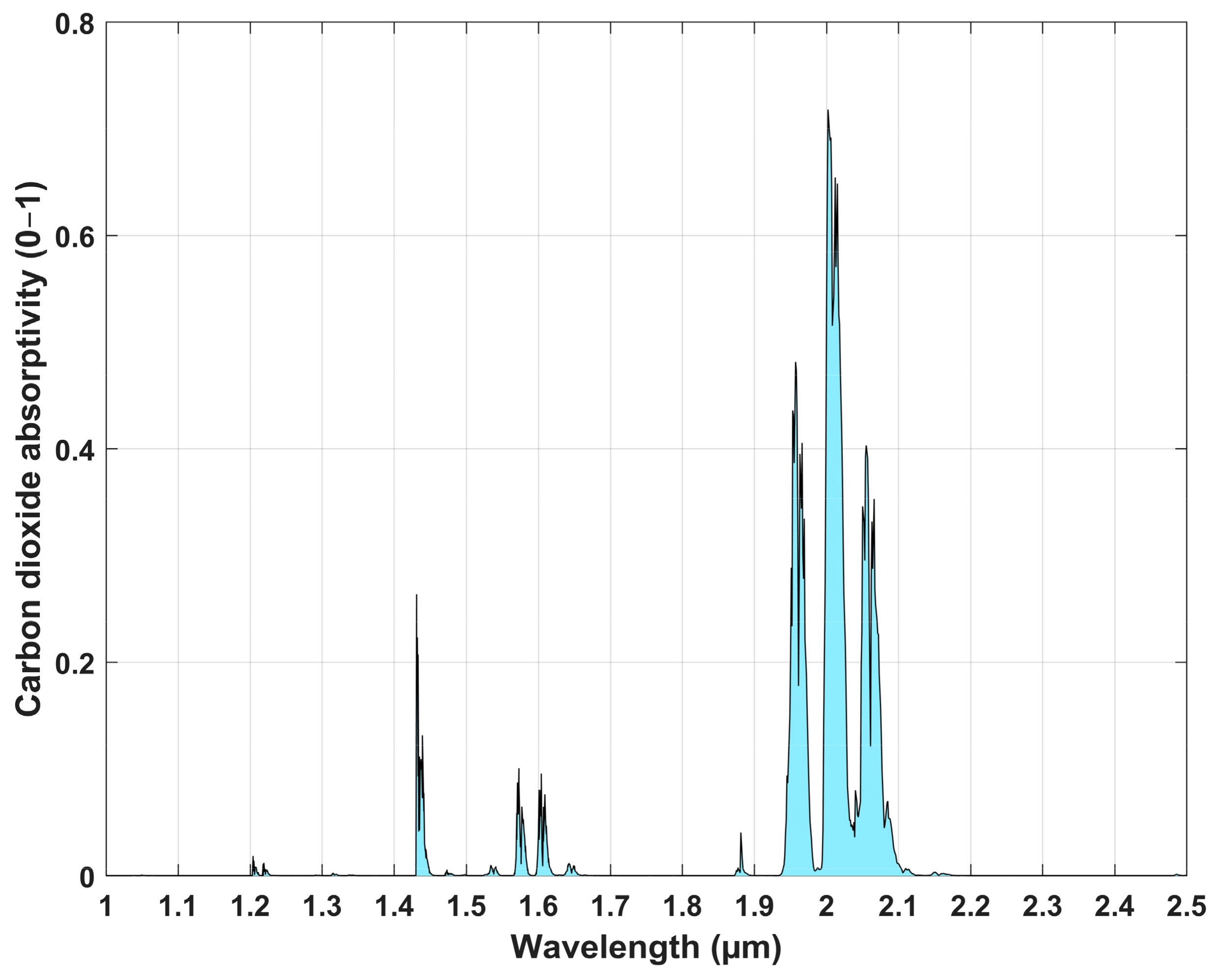
In this work, we exploit the CO2 signatures present in the SWIR spectral range. Figure 1 depicts the absorptivity of carbon dioxide, in the spectral range of 1.0–2.5 µm, obtained by using the MODTRAN (MODerate resolution atmospheric TRANsmission) radiative transfer model [39] and considering the current concentration in the atmosphere of about 400 ppm. The gas shows weak absorptions in the range of 1.4–1.6 µm and strong absorptions in the range of 1.9–2.1 µm (Figure 1). In particular, the analysis performed in the paper focuses on the absorption around 2.06 µm and takes advantage from simulations carried out from version 6.0 of the MODTRAN code.
This chapter firstly describes performed model simulations and the selection of PRISMA channels for retrieval purposes; then, the choice of weight coefficients, for the CIBR index calculation, is discussed with the aim of reducing the influence of the water absorption in the computation of index values. Moreover, the conversion from CIBR values to XCO2 estimations is presented and finally, the limits and applicability of the methodology are reported.
2.1. MODTRAN Simulations and Selection of PRISMA Channels
The first set of five model simulations were performed by using the MODTRAN radiative transfer model with the aim of selecting the best PRISMA channels for CO2 retrieval purposes. Specifically, simulations were performed, with varying XCO2 values and maintaining fixed all other parameters (see Table 1); CO2 concentration profiles were assumed to have constant values in vertical direction, in accordance with the model “US standard 1976”.
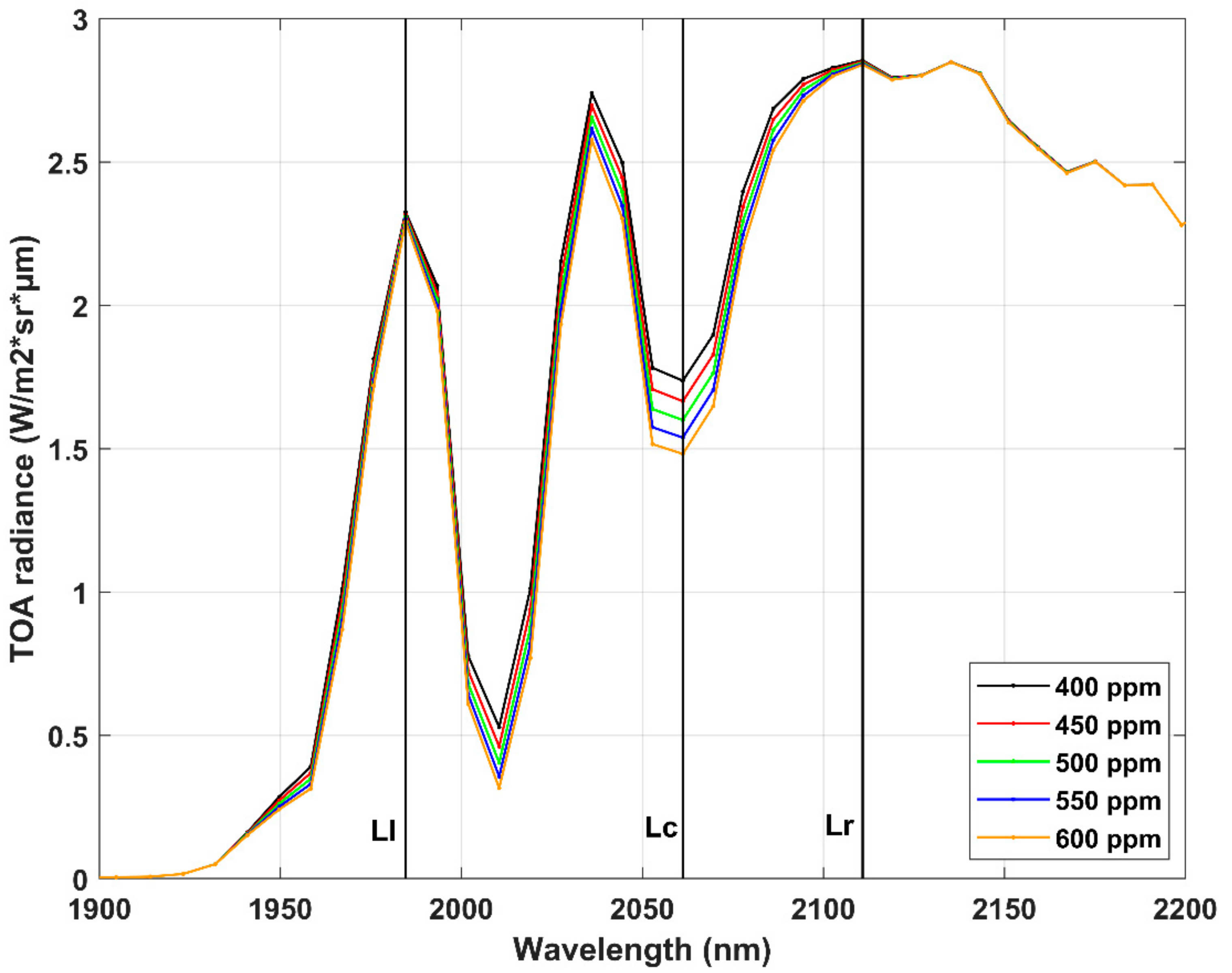
The model runs were at a very high spectral resolution (1 cm−1) and the resulting TOA (Top Of Atmosphere) radiance was convolved on PRISMA channels (see resulting profiles in the Figure 2). The FWHM (Full Width at Half Maximum) of channels in the considered spectral portion 1900–2200 nm is within the range 10–12 nm. Figure 2 also reports positions of the channel most affected by CO2 absorption (central vertical line at 2061 nm) and the immediately adjacent channels not affected by the gas absorption (at 1985 and 2111 nm).
The CIBR index is defined as follows:
where Lc is the radiance at the PRISMA channel #115 (2061 nm), Ll is the radiance at channel #106 (1985 nm) and Lr is the radiance at channel #121 (2111 nm); A and B are weight coefficients, linked by the relationship A + B = 1, and its values will be discussed in Section 2.2.
2.2. Selection of the Weight Coefficients A and B to Reduce the Water Vapor Influence
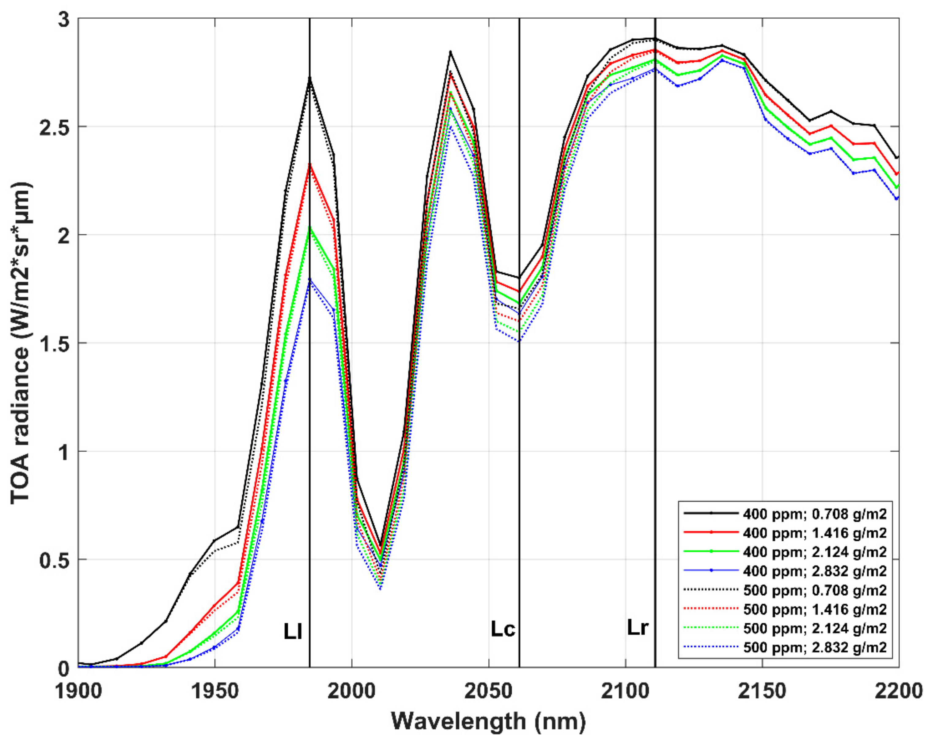
The weighting factors A and B in Equation (1) generally represent, in CIBR technique applications, the spectral distances of “shoulder” wavelengths with no absorption from the channel affected by gas absorption [40]. In the present study, the weighting factors are defined and exploited to mitigate effects of the water absorption on spectral profiles. In fact, the spectral region in the range of 1900–2200 nm is strongly affected by water vapor absorptions that reduce radiance values achieved by remote sensors; it is crucial to evaluate these effects to discriminate absorptions due to H2O or CO2 and correctly estimate XCO2 enhancements. Hence, the model simulations described above were repeated for several H2O column amounts: 0.708, 1.416 (US standard 1976), 2.124 and 2.832 g/m2. Figure 3 shows resulting spectral profiles for considered H2O concentrations and for CO2 column-averaged values of 400 and 500 ppm.
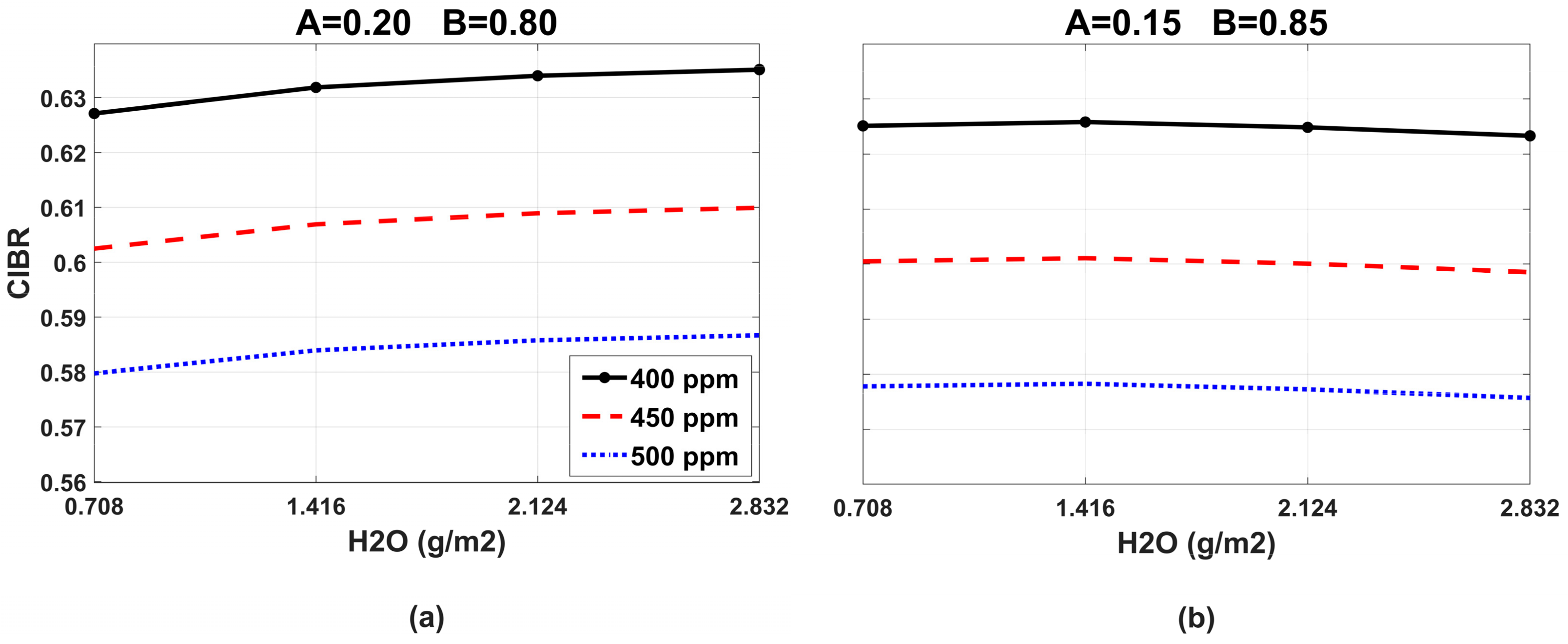
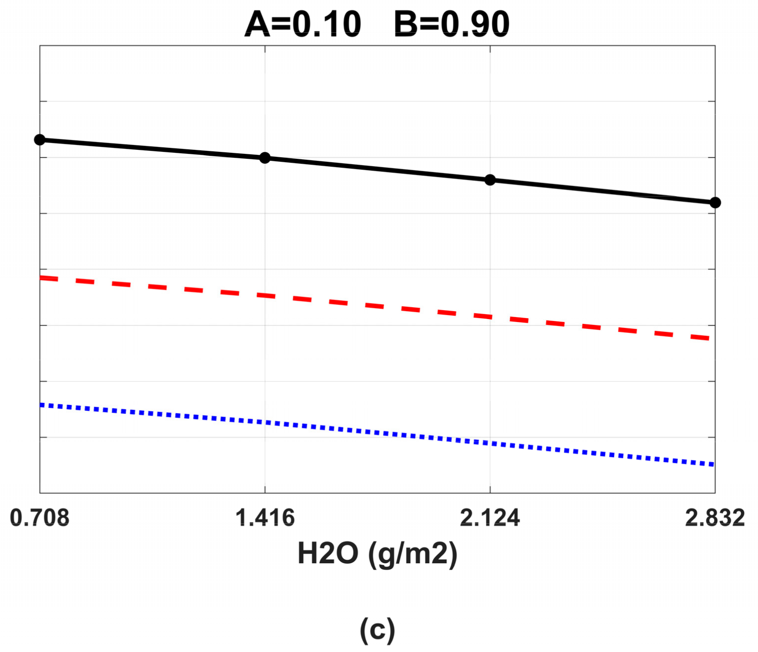
Absorption effects of water vapor are evident for the entire considered spectral range and in particular for wavelengths less than 2000 nm. The method used for reducing water effects acts on the choice of weight coefficients A and B, so that the decrease or increase in CIBR values does not depend on the water concentration. A set of coefficient values was experimentally used by varying the A value in the range of 0.05–0.50 (at steps of 0.05) and the B value in the range of 0.50–0.95. The CIBR dependence on H2O column amounts results in the minimal assignment of the values of 0.15 and 0.85 for A and B coefficients, respectively (Figure 4b). The CIBR parameter as a function of the H2O column amount is shown for only three different combinations of the two coefficients (Figure 4).
2.3. Conversion from CIBR to XCO2 by Means of MODTRAN Simulations
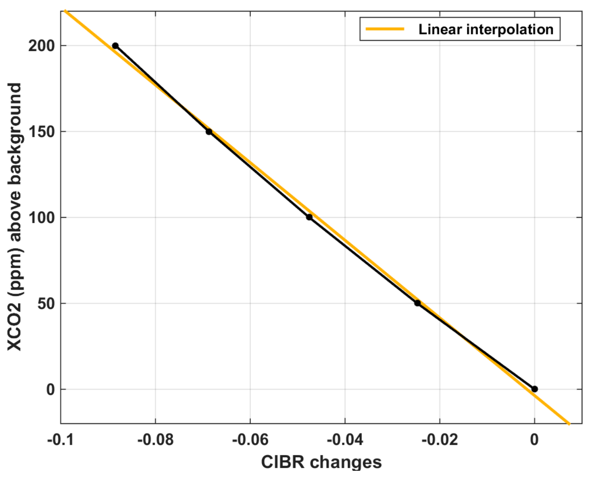
The conversion from CIBR values to XCO2 estimations, in parts per million, is a crucial point. The set of model simulations described in Section 2.1 is used to link changes of CIBR values to XCO2 enhancements. Results show an almost linear relationship between the two parameters (see Figure 5). Specifically, it was revealed that an enhancement of 50 ppm in XCO2 leads to a reduction of 0.0234 for the CIBR value; however, such a conversion factor only links changes of the two parameters. In order to fix the reference CIBR value corresponding to the background CO2 column-averaged value of 400 ppm, its modal value in the PRISMA scene was considered and calculated. Then, CIBR deviations from its modal value were attributed to carbon dioxide emissions, according to the estimated conversion factor under the linear hypothesis.
2.4. Minimum TOA Radiance Values and Confidence Mask
Low values of ground reflectance, in standard conditions of surface temperature, lead to low values of TOA radiance in the SWIR spectral range. MODTRAN model experiments were performed considering a constant reflectance equal to 0.1 that determines radiance values around 2 Wm−2sr−1µm−1 (see Figure 2) for the PRISMA channels employed in the CIBR index calculation. Therefore, in the present study we did not consider physical conditions with surface reflectance values less than 0.1; for this reason, the confidence mask of retrieval results is defined for values of Lr greater than 2 Wm−2sr−1µm−1.
3. Applications
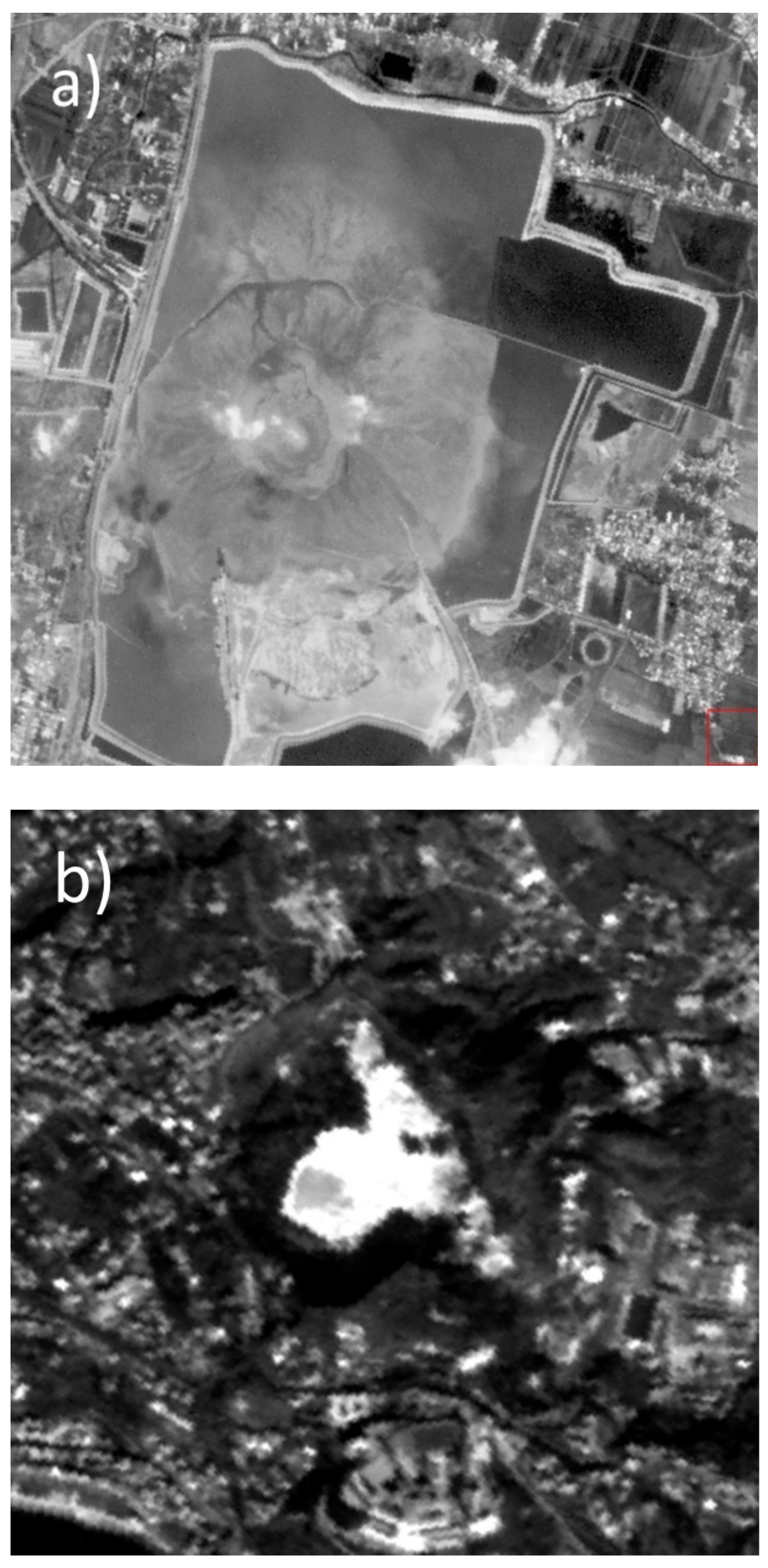
The sites selected for testing the method are the LUSI volcanic area (Indonesia) and the Solfatara area in the caldera of Campi Flegrei (Italy) (see Figure 6). Both areas are characterized by gas emissions but have very different geological structures [41,42].
Table 2 lists the characteristics of the test sites and the PRISMA acquisitions considered for CO2 emissions retrieval.
3.1. Results of Retrieval
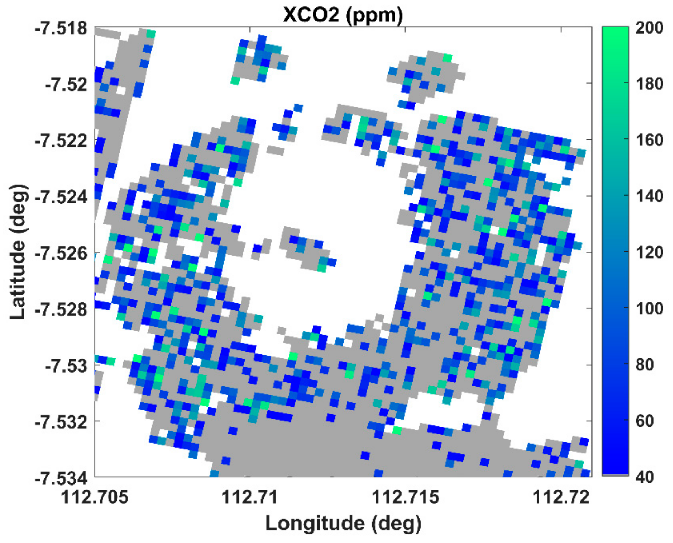
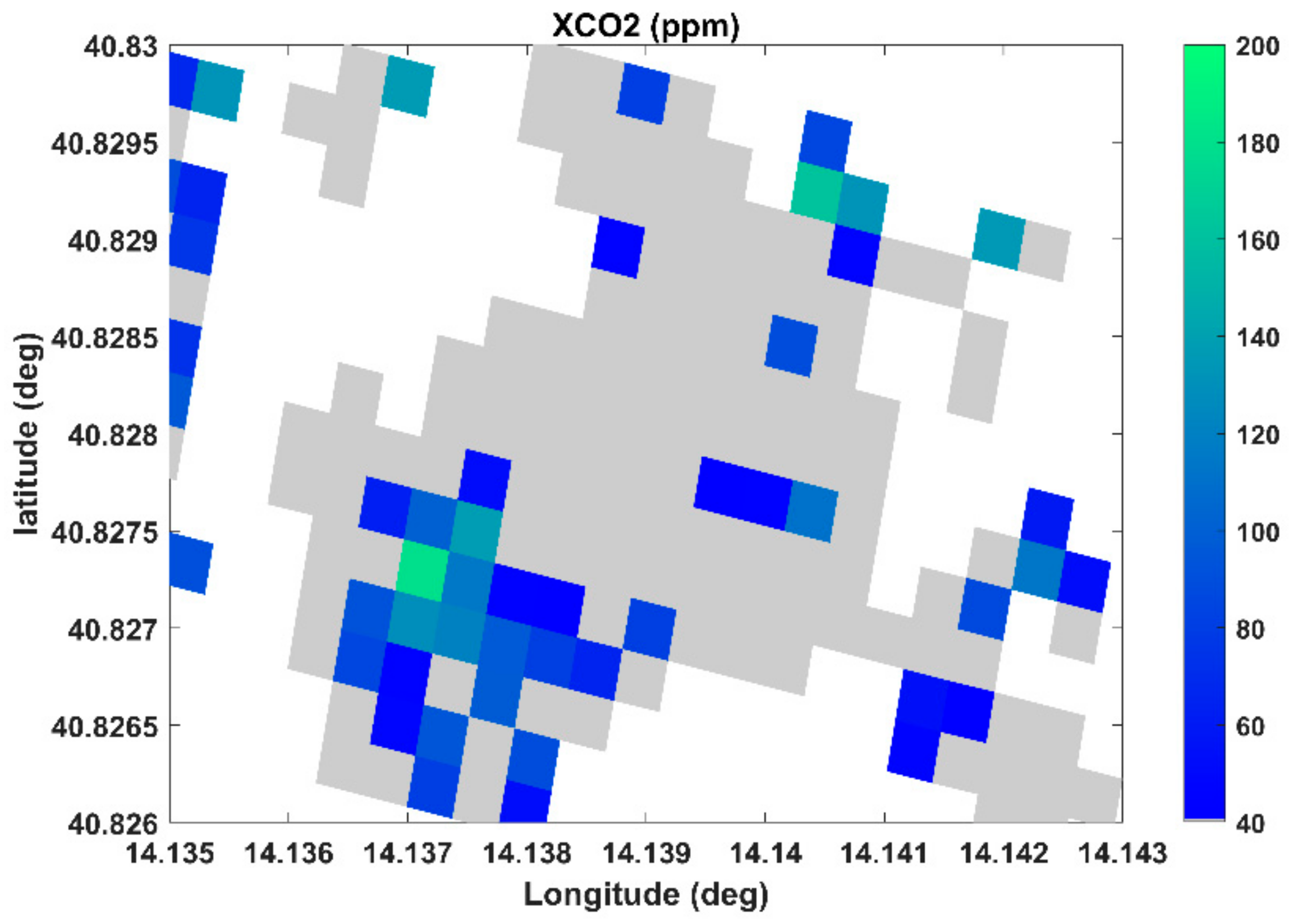
The methodology developed in the present study was applied to the two considered test cases. The results of XCO2 retrieval are depicted in Figure 7 and Figure 8 for LUSI and Solfatara, respectively. White areas represent regions with Lr radiance less than 2 Wm−2sr−1µm−1 (so not considered for the retrieval), while grey areas include regions with XCO2 enhancement values up to 40 ppm, which is the minimum detectable value, as discussed in Section 3.2.
3.2. Errors Evaluation and Minimum Value of XCO2
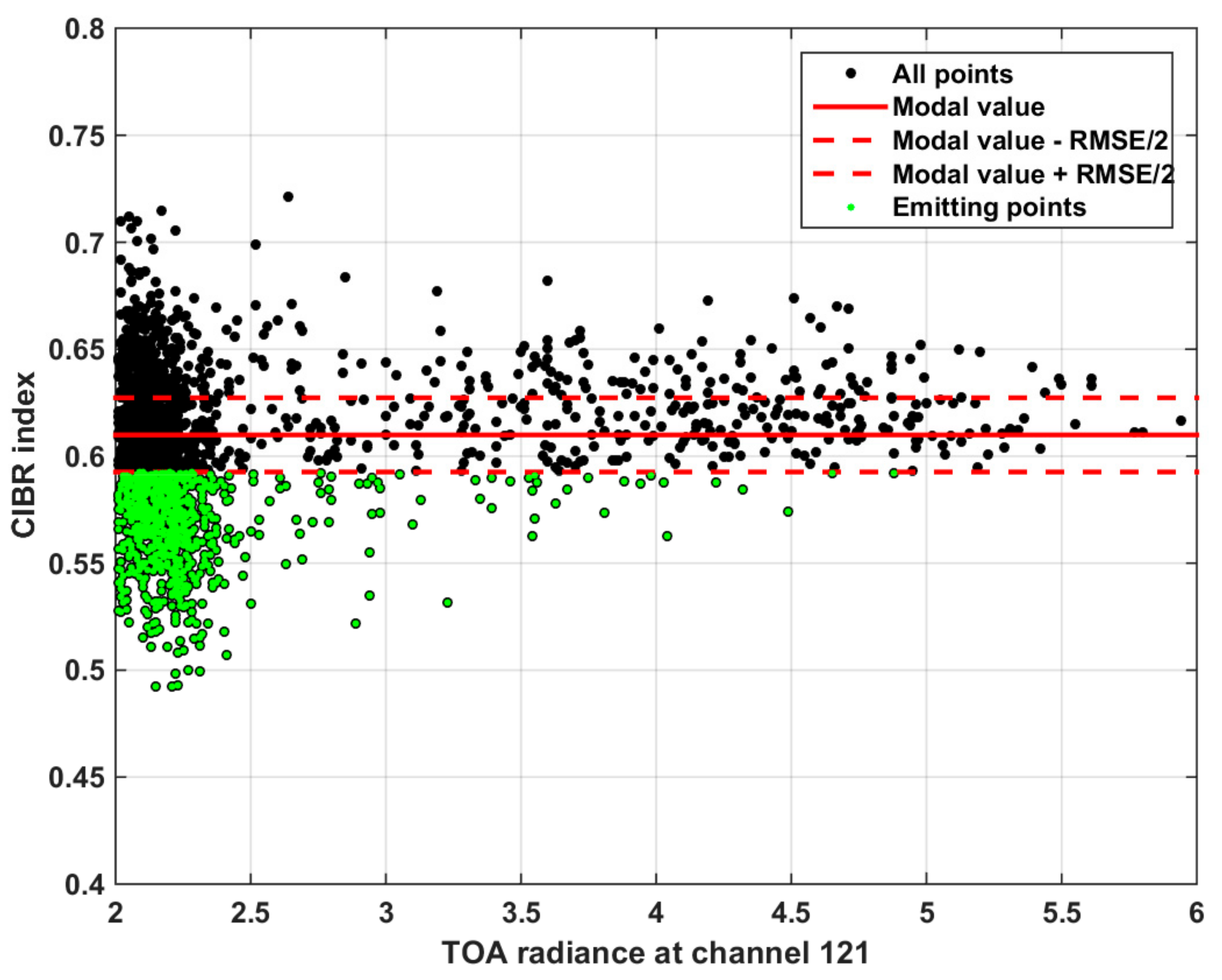
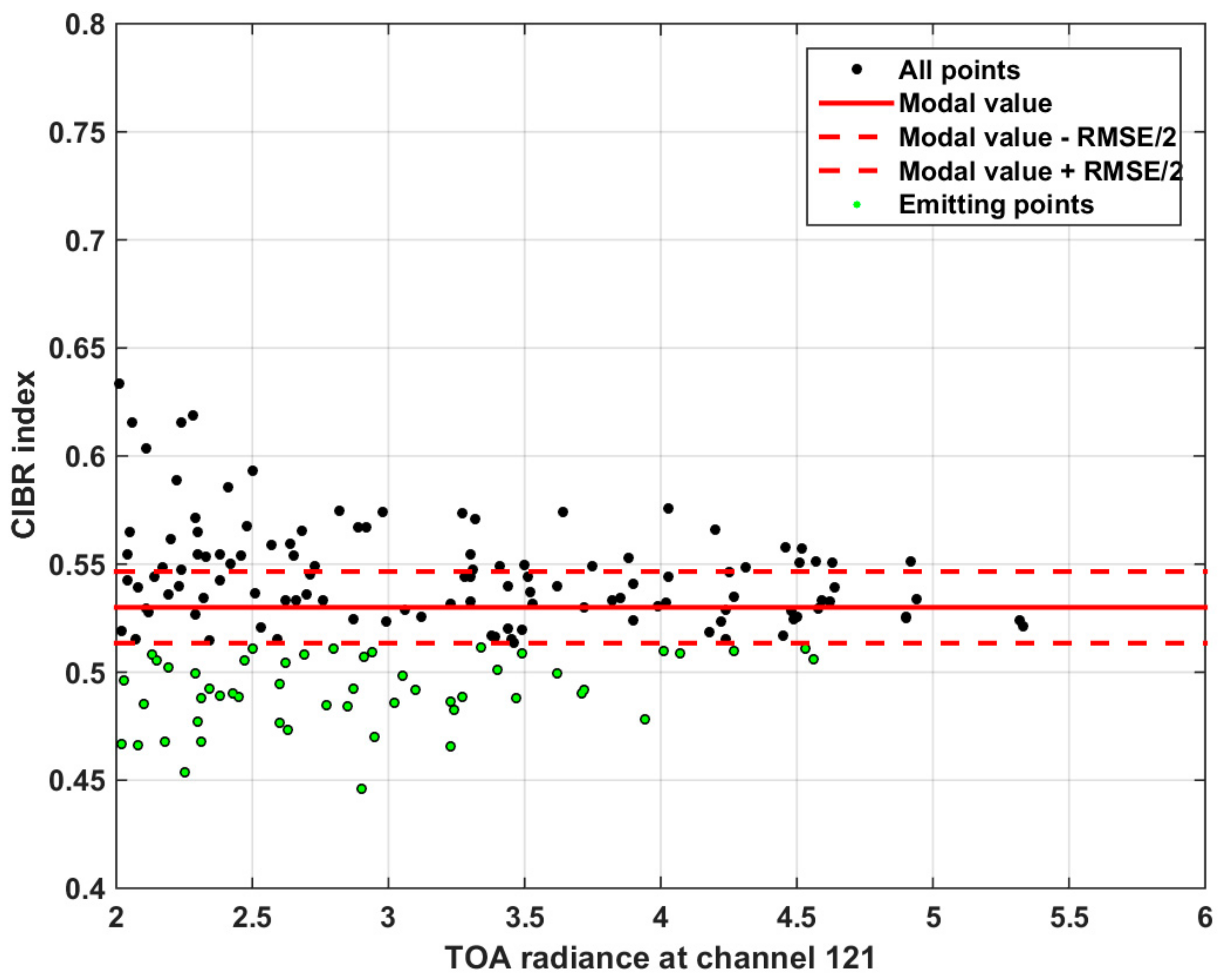
The errors and limits of the retrieval method are also evaluated considering the relationship between the CIBR values and the TOA radiance at the channel #121 (2111 nm) that is less affected by CO2 and H2O absorptions and so is mainly linked to surface reflectance. Figure 9 and Figure 10 show scatter plots between the two considered parameters for the LUSI and Solfatara sites, respectively.
For both test cases, only points with a TOA121 radiance greater than 2 Wm−2sr−1µm−1 were considered. Regarding the LUSI test case, the modal value of CIBR results are equal to 0.610 with a RMSE/2 equal to 0.0174. Considering the conversion factor of 0.0234 for a XCO2 enhancement of 50 ppm, the minimum detectable value results are about 37 ppm. For the Solfatara test case, the modal value of CIBR results are equal to 0.530 with a RMSE/2 equal to 0.0165, leading to a minimum detectable value of about 35 ppm.
4. Discussion
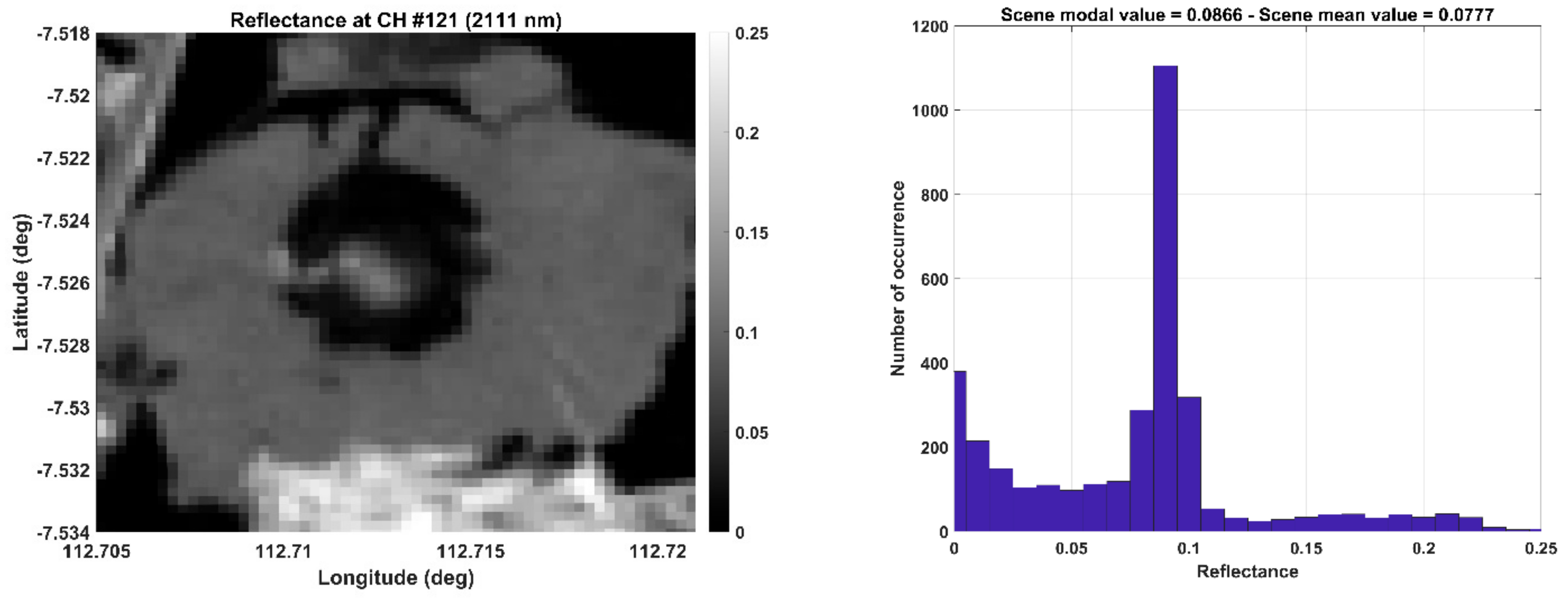
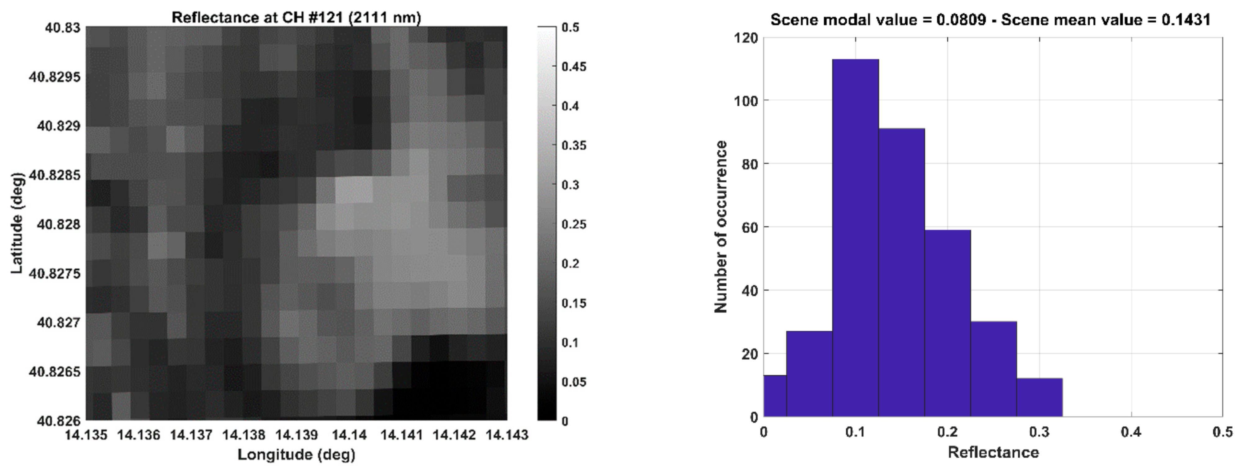
In this study, the surface reflectance used in MODTRAN simulations is considered spatially constant and is equal to 0.1. Firstly, this threshold value was selected to consider TOA radiance values ~5–10 times greater than sensor noise and avoid large errors in the CIBR index calculation. Secondly, although this technique is robust with respect to variations in soil composition, a non-case-dependent algorithm must consider variations of surface reflectance values with respect to space and wavelength. For the LUSI test case, the mud area emitting CO2 is characterized by a spatially constant value of reflectance of about 0.09 (Figure 11); this hypothesis is weaker for the Solfatara case, where the emitting area has reflectance values up to 0.3–0.4 (Figure 12). Finally, the comparison between XCO2 enhancements and reflectance values do not show any correlation.
The effects of atmospheric aerosols were also tested by performing several MODTRAN simulations. Specifically, AOD (Aerosol Optical Depth) values measured from the AERONET network close to test sites, at the same time of PRISMA acquisitions, have been used as input for radiative model runs. The “Rural” and “Urban” parametrization aerosol models, were considered, with AOD values of 0.295 and 0.102 for the LUSI and Solfatara sites, respectively. The comparison with the “No aerosol” parametrization highlighted that simulated TOA radiance results were very different in the spectral range of 0.4–1.0 µm but almost identical for longer wavelengths. Furthermore, the considered test sites are characterized by fumarolic activities with little formation of volcanic aerosols; therefore, as a first approximation, aerosol effects can be neglected in the XCO2 retrieval using the 2 µm band.
A critical point of this work regards the validation of the method itself comparing the results with other types of data; a comparison with in situ measurements would be very useful. Nevertheless, the main objective of the present work is to define a simple methodology to detect and quantify CO2 emissions by means of SWIR channels of the PRISMA sensor. Further works for validation purposes could be carried out, including enlarging the PRISMA dataset, calculating gas fluxes, and finding proximal data such as by gas sampling instruments on drones.
5. Conclusions
In this work, a methodology for CO2 emission retrieval at the local scale, arranged using hyperspectral PRISMA data, was presented and tested. The spatial resolution of gas enhancement estimates is about 30 m, corresponding to the ground sampling distance of the space sensor in SWIR channels. The method is based on the CIBR technique, and TOA radiances obtained from the MODTRAN model simulations were convolved on PRISMA channels. Simulations were used to select the best channels for CO2 retrieval purposes and other parameters characterizing the technique. The method seems to be able to retrieve CO2 enhancements from different gas sources with a minimum detectable XCO2 value, above the background, of about 40 ppm. The methodology can be applied, with satisfactory success, for medium/strong emissions and over soils with a reflectance greater than 0.1.
Author Contributions
Conceptualization, V.R. and M.F.B.; methodology, V.R. and C.S.; software V.R.; investigation, V.R.; data curation, V.R. and M.S.; writing—original draft preparation, V.R.; writing—review and editing, M.S. and M.F.B.; supervision, M.F.B. All authors have read and agreed to the published version of the manuscript.
Funding
This research received no external funding.
Institutional Review Board Statement
Not applicable.
Informed Consent Statement
Not applicable.
Acknowledgments
Thanks to the Italian Space Agency for providing the PRISMA data.
Conflicts of Interest
The author declares no conflict of interest.
References
- Masson-Delmotte, V.; Zhai, P.; Pirani, A.; Connors, S.L.; Péan, C.; Berger, C.; Caud, N.; Chen, Y.; Goldfarb, L.; Gomis, M.I.; et al. IPCC, 2021: Summary for Policymakers. In Climate Change 2021: The Physical Science Basis. Contribution of Working Group I to the Sixth Assessment Report of the Intergovernmental Panel on Climate Change; Cambridge University Press: Cambridge, UK, 2021; in press. [Google Scholar]
- Masson-Delmotte, V.; Zhai, P.; Pörtner, H.O.; Roberts, D.; Skea, J.; Shukla, P.R.; Pirani, A.; Moufouma-Okia, W.; Péan, C.; Pidcock, R.; et al. IPCC, 2018: Summary for Policymakers. In Global Warming of 1.5 °C. An IPCC Special Report on the Impacts of Global Warming of 1.5 °C above Pre-Industrial Levels and Related Global Greenhouse Gas Emission Pathways, in the Context of Strengthening the Global Response to the Threat of Climate Change, Sustainable Development, and Efforts to Eradicate Poverty; World Meteorological Organization: Geneva, Switzerland, 2018; p. 32. [Google Scholar]
- Kuze, A.; Suto, H.; Nakajima, M.; Hamazaki, T. Thermal and near infrared sensor for carbon observation Fourier-transform spectrometer on the Greenhouse Gases Observing Satellite for greenhouse gases monitoring. Appl. Opt. 2009, 48, 6716–6733. [Google Scholar] [CrossRef] [PubMed]
- Orbiting Carbon Observatory-2 (OCO-2). Available online: https://ocov2.jpl.nasa.gov/ (accessed on 2 November 2021).
- Frankenberg, C.; Pollock, R.; Lee, R.A.M.; Rosenberg, R.; Blavier, J.F.; Crisp, D.; O’Dell, C.W.; Osterman, G.B.; Roehl, C.; Wennberg, P.O.; et al. The Orbiting Carbon Observatory (OCO-2): Spectrometer performance evaluation using pre-launch direct sun measurements. Atmos. Meas. Tech. 2015, 8, 301–313. [Google Scholar] [CrossRef] [Green Version]
- Miller, S.M.; Michalak, A.M.; Yadav, V.; Tadić, J.M. Characterizing biospheric carbon balance using CO2 observations from the OCO-2 satellite. Atmos. Chem. Phys. 2018, 18, 6785–6799. [Google Scholar] [CrossRef] [Green Version]
- Schwandneret, F.M.; Gunson, M.R.; Miller, C.E.; Carn, S.A.; Eldering, A.; Krings, T.; Verhulst, K.R.; Schimel, D.S.; Nguyen, H.M.; Crisp, D.; et al. Spaceborne detection of localized carbon dioxide sources. Science 2017, 358, eaam5782. [Google Scholar] [CrossRef] [Green Version]
- Yang, D.; Liu, Y.; Cai, Z.; Chen, X.; Yao, L.; Lu, D. First Global Carbon Dioxide Maps Produced from TanSat Measurements. Adv. Atmos. Sci. 2018, 35, 621. [Google Scholar] [CrossRef]
- Orbiting Carbon Observatory-3 (OCO-3). Available online: https://www.jpl.nasa.gov/missions/orbiting-carbon-observatory-3-oco-3 (accessed on 2 November 2021).
- Eldering, A.; Taylor, T.E.; O’Dell, C.W.; Pavlick, R. The OCO-3 mission: Measurement objectives and expected performance based on 1 year of simulated data. Atmos. Meas. Tech. 2019, 12, 2341–2370. [Google Scholar] [CrossRef] [Green Version]
- Griffin, M.K.; Burke, H.K.; Kerekes, J.P. Understanding radiative transfer in the midwave infrared, a precursor to full spectrum atmospheric compensation. Proc. SPIE 2004, 5425, 348. [Google Scholar]
- Romaniello, V.; Spinetti, C.; Silvestri, M.; Buongiorno, M.F. A Sensitivity Study of the 4.8 µm Carbon Dioxide Absorption Band in the MWIR Spectral Range. Remote Sens. 2020, 12, 172. [Google Scholar] [CrossRef] [Green Version]
- Hook, S.J.; Myers, J.J.; Thome, K.J.; Fitzgerald, M.; Kahle, A.B. The MODIS/ASTER airborne simulator (MASTER)—A new instrument for earth science studies. Remote Sens. Environ. 2001, 76, 93–102. [Google Scholar] [CrossRef]
- Spinetti, C.; Carrere, V.; Buongiorno, M.F.; Sutton, A.J.; Elias, T. Carbon Dioxide of Kilauea Volcanic Plume Retrieved by Means of Airborne Hyperspectral Remote Sensing. Remote Sens. Environ. 2008, 112, 3192–3199. [Google Scholar] [CrossRef]
- Heymann, J.; Reuter, M.; Buchwitz, M.; Schneising, O.; Bovensmann, H.; Burrows, J.P.; Massart, S.; Kaiser, J.W.; Crisp, D.; O’Dell, C.W. CO2 emission of Indonesian fires in 2015 estimated from satellite-derived atmospheric CO2 concentrations. Geophys. Res. Lett. 2017, 44, 1537–1544. [Google Scholar] [CrossRef]
- Nassar, R.; Hill, T.G.; McLinden, C.A.; Wunch, D.; Jones, B.A.; Crisp, D. Quantifying CO2 emissions from individual power plants from space. Geophys. Res. Lett. 2017, 44, 10045–10053. [Google Scholar] [CrossRef] [Green Version]
- Niyogi, D.; Jamshidi, S.; Smith, D.; Kellner, O. Evapotranspiration Climatology of Indiana, USA Using In Situ and Remotely Sensed Products. J. Appl. Meteorol. Clim. 2020, 59, 2093–2111. [Google Scholar] [CrossRef]
- Hernández-Clemente, R.; Hornero, A.; Mottus, M.; Penuelas, J.; González-Dugo, V.; Jiménez, J.C.; Suárez, L.; Alonso, L.; Zarco-Tejada, P.J. Early Diagnosis of Vegetation Health from High-Resolution Hyperspectral and Thermal Imagery: Lessons Learned From Empirical Relationships and Radiative Transfer Modelling. Curr. For. Rep. 2019, 5, 169–183. [Google Scholar] [CrossRef] [Green Version]
- Jamshidi, S.; Zand-Parsa, S.; Niyogi, D. Assessing Crop Water Stress Index for Citrus Using In-Situ Measurements, Landsat, and Sentinel-2 Data. Int. J. Remote Sens. 2020, 42, 1893–1916. [Google Scholar] [CrossRef]
- Lorenz, S.; Zimmermann, R.; Gloaguen, R. The Need for Accurate Geometric and Radiometric Corrections of Drone-Borne Hyperspectral Data for Mineral Exploration: MEPHySTo—A Toolbox for Pre-Processing Drone-Borne Hyperspectral Data. Remote Sens. 2017, 9, 88. [Google Scholar] [CrossRef] [Green Version]
- Ramakrishnan, D.; Bharti, R. Hyperspectral remote sensing and geological applications. Curr. Sci. 2015, 108, 879–891. [Google Scholar]
- Jamshidi, S.; Zand-Parsa, S.; Jahromi, M.N.; Niyogi, D. Application of A Simple Landsat-MODIS Fusion Model to Estimate Evapotranspiration over A Heterogeneous Sparse Vegetation Region. Remote Sens. 2019, 11, 741. [Google Scholar] [CrossRef] [Green Version]
- Jamshidi, S.; Zand-Parsa, S.; Pakparvar, M.; Niyogi, D. Evaluation of Evapotranspiration over a Semiarid Region Using Multiresolution Data Sources. J. Hydrometeorol. 2019, 20, 947–964. [Google Scholar] [CrossRef]
- Chander, S.; Gujrati, A.; Krishna, A.V.; Sahay, A.; Singh, R. Remote sensing of inland water quality: A hyperspectral perspective. In Hyperspectral Remote Sensing; Elsevier: Amsterdam, The Netherlands, 2020; pp. 197–219. [Google Scholar]
- Bagheri, N.; Mohamadi-Monavar, H.; Azizi, A.; Ghasemi, A. Detection of Fire Blight disease in pear trees by hyperspectral data. Eur. J. Remote Sens. 2017, 51, 1–10. [Google Scholar] [CrossRef] [Green Version]
- Veraverbeke, S.; Dennison, P.; Gitas, I.Z.; Hulley, G.C.; Kalashnikova, O.V.; Katagis, T.; Kuai, L.; Meng, R.; Roberts, D.A.; Stavros, E.N. Hyperspectral remote sensing of fire: State-of-the-art and future perspectives. Remote Sens. Environ. 2018, 216, 105–121. [Google Scholar] [CrossRef]
- Dennison, P.; Roberts, D.A. Daytime fire detection using airborne hyperspectral data. Remote Sens. Environ. 2009, 113, 1646–1657. [Google Scholar] [CrossRef]
- Loizzo, R.; Guarini, R.; Longo, F.; Scopa, T.; Formaro, R.; Facchinetti, C.; Varacalli, G. Prisma: The Italian Hyperspectral Mission. In Proceedings of the IGARSS 2018 IEEE International Geoscience and Remote Sensing Symposium, Valencia, Spain, 22–27 July 2018; pp. 175–178. [Google Scholar]
- Giardino, C.; Bresciani, M.; Braga, F.; Fabbretto, A.; Ghirardi, N.; Pepe, M.; Gianinetto, M.; Colombo, R.; Cogliati, S.; Ghebrehiwot, S.; et al. First Evaluation of PRISMA Level 1 Data for Water Applications. Sensors 2020, 20, 4553. [Google Scholar] [CrossRef] [PubMed]
- Casa, R.; Pignatti, S.; Pascucci, S.; Ionca, V.; Mzid, N.; Veretelnikova, I. Assessment of PRISMA imaging spectrometer data for the estimation of topsoil properties of agronomic interest at the field scale. In Proceedings of the22nd EGU General Assembly Conference, Wien, Austria, 4–8 May 2020; p. 6728. [Google Scholar]
- Romaniello, V.; Silvestri, M.; Buongiorno, M.F.; Musacchio, M. Comparison of PRISMA Data with Model Simulations, Hyperion Reflectance and Field Spectrometer Measurements on ‘Piano delle Concazze’ (Mt. Etna, Italy). Sensors 2020, 20, 7224. [Google Scholar] [CrossRef]
- Irakulis-Loitxate, I.; Guanter, L.; Liu, Y.N.; Varon, D.J.; Maasakkers, J.D.; Zhang, Y.; Jacob, D.J.; Chulakadabba, A.; Thorpe, A.K.; Duren, R.M.; et al. Satellite-based survey of extreme methane emissions in the Permian basin. Sci. Adv. 2021, 7, eabf4507. [Google Scholar] [CrossRef] [PubMed]
- Cusworth, D.H.; Duren, R.M.; Thorpe, A.K.; Eastwood, M.L.; Green, R.O.; Dennison, P.E.; Frankenberg, C.; Heckler, J.W.; Asner, G.P.; Miller, C.E. Quantifying global power plant carbon dioxide emissions with imaging spectroscopy. AGU Adv. 2021, 2, e2020AV000350. [Google Scholar] [CrossRef]
- Guanter, L.; Irakulis-Loitxate, I.; Gorroño, J.; Sánchez-García, E.; Cusworth, D.H.; Varon, D.J.; Colombo, R.; Cogliati, S. Mapping methane point emissions with the PRISMA spaceborne imaging spectrometer. Remote Sens. Environ. 2021, 265, 112671. [Google Scholar] [CrossRef]
- Thorpe, A.K.; Frankenberg, C.; Thompson, D.R.; Duren, R.M.; Aubrey, A.D.; Bue, B.D.; Dennison, P.E.; Green, R.O.; Gerilowski, K.; Krings, T.; et al. Airborne DOAS retrievals of methane, carbon dioxide, and water vapor concentrations at high spatial resolution: Application to AVIRIS-NG. Atmos. Meas. Tech. 2017, 10, 3833–3850. [Google Scholar] [CrossRef] [Green Version]
- Foote, M.D.; Dennison, P.E.; Thorpe, A.K.; Thompson, D.R.; Jongaramrungruang, S.; Frankenberg, C.; Joshi, S.C. Fast and accurate retrieval of methane concentration from imaging spectrometer data using sparsity prior. IEEE Trans. Geosci. Remote Sens. 2020, 58, 6480–6492. [Google Scholar] [CrossRef] [Green Version]
- Carrere, V.; Conel, J.E. Recovery of atmospheric water vapor total column abundance from imaging spectrometer data around 940 nm—Sensitivity analysis and application to airborne visible/infrared imaging spectrometer (AVIRIS) data. Remote Sens. Environ. 1993, 44, 179–204. [Google Scholar] [CrossRef]
- Mishra, M.K.; Gupta, A.; John, J.; Shukla, B.P.; Dennison, P.; Srivastava, S.S.; Dhar, D.; Kaushik, N.K.; Misra, A. Retrieval of atmospheric parameters and data-processing algorithms for AVIRIS-NG Indian campaign data. Curr. Sci. 2019, 116, 1–12. [Google Scholar] [CrossRef]
- MODTRAN Computer Code. Available online: http://modtran.spectral.com/ (accessed on 2 November 2021).
- Amici, S.; Piscini, A. Exploring PRISMA Scene for Fire Detection: Case Study of 2019 Bushfires in Ben Halls Gap National Park, NSW, Australia. Remote Sens. 2021, 13, 1410. [Google Scholar] [CrossRef]
- Mazzini, A.; Sciarra, A.; Etiope, G.; Sadavarte, P.; Houweling, S.; Pandey, S.; Husein, A. Relevant methane emission to the atmosphere from a geological gas manifestation. Sci. Rep. 2021, 11, 4138. [Google Scholar] [CrossRef] [PubMed]
- Chiodini, G.; Caliro, S.; Avino, R.; Bini, G.; Giudicepietro, F.; De Cesare, W.; Tripaldi, S.; Ricciolino, P.; Aiuppa, A.; Cardellini, C.; et al. Hydrothermal pressure-temperature control on CO2 emissions and seismicity at Campi Flegrei (Italy). J. Volcanol. Geotherm. Res. 2021, 414, 107245. [Google Scholar] [CrossRef]
Figure 1.
Carbon dioxide absorption bands in the SWIR spectral range.

Figure 2.
Simulated TOA spectral profiles convolved on PRISMA channels for several CO2 column-averaged values (400, 450, 500, 550, 600 ppm) and the standard H2O column amount corresponding to 1.416 g/m2 (US standard 1976).
Figure 2.
Simulated TOA spectral profiles convolved on PRISMA channels for several CO2 column-averaged values (400, 450, 500, 550, 600 ppm) and the standard H2O column amount corresponding to 1.416 g/m2 (US standard 1976).

Figure 3.
Simulated TOA spectral profiles convolved on PRISMA channels, for two CO2 column-averaged values (400, 500 ppm) and four H2O column amounts (0.708, 1.416, 2.124, 2.832 g/m2).
Figure 3.
Simulated TOA spectral profiles convolved on PRISMA channels, for two CO2 column-averaged values (400, 500 ppm) and four H2O column amounts (0.708, 1.416, 2.124, 2.832 g/m2).

Figure 4.
CIBR index simulations for three different combinations of A and B weight coefficients: A = 0.20, B = 0.80 (a); A = 0.15, B = 0.85 (b); A = 0.10, B = 0.90 (c).
Figure 4.
CIBR index simulations for three different combinations of A and B weight coefficients: A = 0.20, B = 0.80 (a); A = 0.15, B = 0.85 (b); A = 0.10, B = 0.90 (c).


Figure 5.
Modelled relationship between CIBR changes and XCO2 enhancements.

Figure 6.
PRISMA panchromatic images of LUSI (a) and Solfatara (b) test sites.

Figure 7.
XCO2 (ppm) enhancements on the LUSI test site (Indonesia); PRISMA acquisition on 14 August 2020.
Figure 7.
XCO2 (ppm) enhancements on the LUSI test site (Indonesia); PRISMA acquisition on 14 August 2020.

Figure 8.
XCO2 (ppm) enhancements on the Solfatara test site (Italy); PRISMA acquisition on 18 February 2021.
Figure 8.
XCO2 (ppm) enhancements on the Solfatara test site (Italy); PRISMA acquisition on 18 February 2021.

Figure 9.
Distribution of CIBR values for TOA121 greater than 2 Wm−2sr−1µm−1 (LUSI case study).

Figure 10.
Distribution of CIBR values for TOA121 greater than 2 Wm−2sr−1µm−1 (Solfatara case study).
Figure 10.
Distribution of CIBR values for TOA121 greater than 2 Wm−2sr−1µm−1 (Solfatara case study).

Figure 11.
Reflectance from PRISMA L2D data product on LUSI.

Figure 12.
Reflectance from PRISMA L2D data product on Solfatara.


Table 1.
Input parameters for a set of five MODTRAN runs.
| Input Parameter | Value |
|---|---|
| Spectral range | 0.35–2.55 µm |
| Atmospheric profiles | US standard 1976 |
| Surface temperature | 290 K |
| CO2 concentrations | 400, 450, 500, 550, 600 ppm |
| Ground reflectance | 0.10 |
| Altitude of the first layer | 0 km |
| Altitude of the last layer | 120 km |
| Number of vertical levels | 50 |
| Aerosol | NO |
Table 2.
Test sites and PRISMA dataset.
| Site | Latitude (Deg); Longitude (Deg) | Type of Event | Time of Acquisition |
|---|---|---|---|
| LUSI (Indonesia) | −7.527; 112.711 | H2O, CO2, CH4 degassing | 14 August 2020 |
| Solfatara (Italy) | 40.827; 14.140 | H2O, CO2 degassing | 18 February 2021 |
Publisher’s Note: MDPI stays neutral with regard to jurisdictional claims in published maps and institutional affiliations. |
© 2021 by the authors. Licensee MDPI, Basel, Switzerland. This article is an open access article distributed under the terms and conditions of the Creative Commons Attribution (CC BY) license (https://creativecommons.org/licenses/by/4.0/).
Share and Cite
MDPI and ACS Style
Romaniello, V.; Spinetti, C.; Silvestri, M.; Buongiorno, M.F. A Methodology for CO2 Retrieval Applied to Hyperspectral PRISMA Data. Remote Sens. 2021, 13, 4502. https://doi.org/10.3390/rs13224502
AMA Style
Romaniello V, Spinetti C, Silvestri M, Buongiorno MF. A Methodology for CO2 Retrieval Applied to Hyperspectral PRISMA Data. Remote Sensing. 2021; 13(22):4502. https://doi.org/10.3390/rs13224502
Chicago/Turabian StyleRomaniello, Vito, Claudia Spinetti, Malvina Silvestri, and Maria Fabrizia Buongiorno. 2021. "A Methodology for CO2 Retrieval Applied to Hyperspectral PRISMA Data" Remote Sensing 13, no. 22: 4502. https://doi.org/10.3390/rs13224502
Note that from the first issue of 2016, this journal uses article numbers instead of page numbers. See further details here.