Article

Evaluation of Total Nitrogen in Water via Airborne Hyperspectral Data: Potential of Fractional Order Discretization Algorithm and Discrete Wavelet Transform Analysis

1
Key Laboratory of Smart City and Environment Modelling of Higher Education Institute, College of Resources and Environment Science, Xinjiang University, Urumqi 830046, China
2
MOE Key Laboratory of Oasis Ecology, Xinjiang University, Urumqi 830046, China
3
MNR Technology Innovation Center for Central Asia Geo-Information Exploitation and Utilization, Urumqi 830046, China
4
MNR Key Laboratory for Geo-Environmental Monitoring of Great Bay Area and Guangdong Key Laboratory of Urban Informatics and Shenzhen Key Laboratory of Spatial Smart Sensing and Services, Shenzhen University, Shenzhen 518060, China
*
Author to whom correspondence should be addressed.
Remote Sens. 2021, 13(22), 4643; https://doi.org/10.3390/rs13224643
Submission received: 17 September 2021 / Revised: 11 November 2021 / Accepted: 15 November 2021 / Published: 18 November 2021
(This article belongs to the Section Remote Sensing in Geology, Geomorphology and Hydrology)

Abstract

:
Controlling and managing surface source pollution depends on the rapid monitoring of total nitrogen in water. However, the complex factors affecting water quality (plant shading and suspended matter in water) make direct estimation extremely challenging. Considering the spectral response mechanisms of emergent plants, we coupled discrete wavelet transform (DWT) and fractional order discretization (FOD) techniques with three machine learning models (random forest (RF), bagging algorithm (bagging), and eXtreme Gradient Boosting (XGBoost)) to mine this potential spectral information. A total of 567 models were developed, and airborne hyperspectral data processed with various DWT scales and FOD techniques were compared. The effective information in the hyperspectral reflectance data were better emphasized after DWT processing. After DWT processing the original spectrum (OR), its sensitivity to TN in water was maximally improved by 0.22, and the correlation between FOD and TN in water was optimally increased by 0.57. The transformed spectral information enhanced the TN model accuracy, especially for FOD after DWT. For RF, 82% of the model R2 values improved by 0.02~0.72 compared to the model using FOD spectra; 78.8% of the bagging values improved by 0.01~0.53 and 65.0% of the XGBoost values improved by 0.01~0.64. The XGBoost model with DWT coupled with grey relation analysis (GRA) yielded the best estimation accuracy, with the highest precision of R2 = 0.91 for L6. In conclusion, appropriately scaled DWT analysis can substantially improve the accuracy of extracting TN from UAV hyperspectral images. These outcomes may facilitate the further development of accurate water quality monitoring in sophisticated global waters from drone or satellite hyperspectral data.

1. Introduction

Total nitrogen (TN), as an essential element in water, not only impacts the water quality of inland waters around the world but also has a crucial bearing on the achievement of the United Nations’ sustainable development goals of water conservation and water pollution management [1,2,3]. Water quality issues remain a chronic problem of inland wetland ecosystems [4]. Due to the special characteristics of inland wetland water cycle retardation, environmental pollution caused by unreasonable human production activities and life processes, and the lack of effective monitoring and assessment methods for water bodies, water quality issues such as eutrophication in inland water bodies have arisen, affecting the use value of water, destroying water ecological balance, and threatening food security and human health [5,6,7]. TN complicates the water situation through environmental cascades and related effects [8,9], and controlling the TN content of water in a timely and effective manner has become imperative for the government.
Estimating water quality directly from water surface reflection spectra is by no means easy in complex water environments [10,11]. Emergent plants are one of the monitoring priorities in the aquatic environment [12,13]. The spectral characteristics of emergent vegetation reflect the stoichiometric characteristics of trace elements relevant to water quality; specifically, elements such as nitrogen will affect the structure of plant components, thereby affecting the spectral reflectance of leaves [14,15]. Therefore, the rapid and nondestructive monitoring of water stoichiometric characteristics depends on the spectral information of growing plant leaves. The optimum fit between wetland plant leaf spectral information and the monitoring of water chemometric characteristics was observed for canopy spectra of Phragmites australis among different wetland plant types [16]. P. australis is an emergent plant and its mechanism of nitrogen removal and water purification lies in the fact that it absorbs effective N elements in water through the nitrification of root microorganisms during its growth [17]. TN is an important indicator of plant growth, forming plant components (e.g., chlorophyll) through photosynthesis. The radiation/reflection spectrum of vegetation correlates with chlorophyll concentration, which depicts the electromagnetic oscillations and bending in infrared and visible wavelengths. This emitted oscillation energy is influenced by various structural factors within it, including chlorophyll, water, and cellular structure. [18]. Accordingly, using spectral reflectance as an indirect estimate of TN in water depends on changes in spectral reflectance, primarily attributed to changes in chlorophyll concentration. A study by Asner proposed that spectral reflectance characteristics are influenced by the biochemical and biophysical parameters of plants and are used to estimate the nitrogen content in water [19]. According to previous studies, the correlation is shown in the red spectral reflectance and the blue spectral response to changes in nitrogen [20]. Chlorophyll absorbs strongly in the blue region (400–500 nm) and reflects relatively well in the red spectral region. Hansen and Schjoerring mainly used the blue–green–red band (400–700 nm) to find the best performance indicator for estimating TN concentrations [21]. As the TN concentration increases, the red spectral reflectance becomes more sensitive than the blue spectral response to changes in N [22]. Therefore, the vegetation spectral reflectance characteristics are “redshifted” (630–780 nm) [23], and the reflectance decreases in the red-edge region. This relationship also provides basic theoretical support for estimating TN in water from the spectral reflectance characteristics of wetland vegetation. However, the feasibility of using unmanned aerial vehicle (UAV) hyperspectral data for estimating TN in water is worth studying.
Traditional chemical measurement methods require a certain amount of human labor and material resources and require the collection of samples over a long time, which is not only harmful to plants and unconducive to the restoration and protection of fragile water environments, but is also unsuitable for large-scale application [24]. Remote sensing has been widely and effectively used in recent years as an important means of monitoring the growth of emergent plants to indirectly determine water quality [25]. However, due to atmospheric influences, the complexity of water quality parameters, surface scattering, and aquatic plants, the satellite remote sensing characteristics of water cannot be used to directly determine water quality parameters, which makes it extremely challenging to implement regional water monitoring [26]. In contrast, UAVs, as low-altitude remote sensing platforms, have become important instruments for the indirect monitoring of water quality with the advantages of high efficiency and speed [27,28]. Furthermore, it is highly significant to evaluate the capability of UAV-borne hyperspectral sensors for use in estimating TN in water. Compared with multispectral data, hyperspectral data have abundant spectral information and have great potential for TN monitoring in water [29,30,31]. Nevertheless, the extraction of particular information from hyperspectral data is complicated by many bands, large data volume, and data redundancy, which increase the workload and complexity of data processing and modeling [32,33,34]. It is urgent to develop fast and reliable preprocessing methods to extract useful spectral information.
The enriched spectral information captured by hyperspectral data can obscure valuable information regarding some target variables, which is why many scholars note that preprocessing hyperspectral data is obligatory [31,35,36]. Fractional order discretization (FOD) is one of the frequently applied and more efficient methods for preprocessing hyperspectral data [37]. The FOD has a narrow interval compared to the integer order derivative, which ensures a slow change in the signal-to-noise ratio and provides a spectral enhancement [38,39]. It has the capability to reduce the effect of information loss due to multiple noise partly [40]. Nowadays, FOD has become an acknowledged method in spectral data denoising. Thus, we opt for the FOD method to extract the crucial information of UAV hyperspectral reflectance data as well. Meanwhile, the combination of FOD with other preprocessing algorithms to identify the vital spectral curve information has acquired considerable attention. Bhadra et al. explored the fractional order Savitzky–Golay derivation (FOSGD) for hyperspectral data analysis, where they found that FOSGD could better balance the conflict between resolution and signal intensity and effectively extract information variables [41]. However, studies on FOD-expend are scarce, especially in processing UAV hyperspectral reflectance data. Thus, we proposed FOD combined with discrete wavelet transform (DWT), a new method to denoise hyperspectral data.
DWT is a spectral analysis method for extracting spectral features, and a variety of denoising algorithms (Daubechies N (dbN), Symlets N (symN), Coiflets N (coifN), etc.) have been developed to accomplish different noise elimination effects [42,43,44,45]. Many studies have investigated the processing of hyperspectral data by DWT, which can reveal key target information via low-scale decomposition reconstruction [46,47]. For example, Li et al. rapidly and nondestructively estimated the nitrogen concentration (LNC) of winter wheat at each fertility stage using DWT decomposition of hyperspectral canopy reflectance spectra (450–1350 nm) at 12 scales and obtained the best results at L4 (R2 = 0.91) [47]. Meng et al. applied DWT in the processing of satellite hyperspectral data at 10 scales, and the resulting decomposed and reconstructed first derivative reflectance (FDR) spectra greatly improved the precision of soil moisture prediction at L6 (R2 = 0.83) [48]. However, there is limited research on the application of DWT to airborne hyperspectral data processing. Whether such application is feasible in the study of TN in water and whether it has advantages over the well-known pretreatment methods of emergent vegetation data is worth exploring. In addition, we investigate the effectiveness of the combination of FOD and DWT to process hyperspectral reflectance data based on the existing studies.
Therefore, the paper aims to explore three questions:
(1)
How can DWT analysis potentially extract information from airborne hyperspectral data?
(2)
Which is more advantageous, pretreatment by DWT analysis or pretreatment by DWT combined with FOD?
(3)
Which combination of preprocessing methods and models can best improve the accuracy of hyperspectral prediction of TN in water, thus providing scientific support and reference information for water quality monitoring, other related research, and local precision agriculture?

2. Materials and Methods

2.1. Study Area

The study area is the Ebinur Lake Wetland National Nature Reserve. The Ebinur Lake Oasis (82°33′–83°53′E, 44°31′–45°09′N) is located in the Xinjiang Uygur Autonomous Region of northwestern China (Figure 1). The study area is far from the sea and has a typical continental arid climate (sunshine time is more than 2722 h and annual precipitation is less than 200 mm). The main wetland plants are P. australis and Typha orientalis Presl which are distributed widely and evenly at 0–5 m from the riverbank. The seasonal river confluence in the area that slowly renews the water, coupled with frequent human activities, causes serious eutrophication of the water bodies [49]. However, wetland plants are widely distributed and have an important purifying effect on the eutrophication of the water. To prevent continuous deterioration of the water environment and improve the quality of the ecological environment, the Ebinur Lake Wetland National Nature Reserve was established in 2007 and is included in the list of China’s national nature reserves.

2.2. Data Acquisition

2.2.1. UAV Data Acquisition and Processing

Data were acquired by using the DJI Matrice 600 PRO® (Shenzhen DJI Technology Co., Ltd., Shenzhen, China) hexacopter UAV platform, equipped with a Nano-Hyperspec® hyperspectral sensor (Headwall Photonics Inc., Bolton, MA, USA), it is lightweight (less than 0.6 kg), ranging from 400–1000 nm with 272 spectral bands. The spectral resolution is 6 nm, the resampling interval is 2 nm, and the field of view is 22°. The sensor features a combined global positioning system/inertial measurement unit (GPS/IMU) navigation system that can acquire altitude information for the UAV platform in real time to enhance georeferencing and reflectivity calibration, respectively. To ensure data quality, dark current correction and spectral calibration were performed prior to takeoff. Hyperspectral images were collected at 15:00 (UTC/GMT+08:00) on 15 July 2018, on a clear and windless day. Preprocessing (including radiation correction and splicing) of the UAV data was based on Hyperspec® III (version 3.1) and SpectralView® (version 3.1) software. The extraction of hyperspectral reflectance information was performed with the ENVI5.3 remote sensing image processing platform.

2.2.2. Sample Collection and Experiments

On 15 July 2018, UAV hyperspectral data were acquired, accompanied by field surveys and sampling at 45 water sampling sites along the Aqikesu River. The sampling times met the requirements for single analysis of the river. Most importantly, July is representative of the dry season in the study area, when the river is narrow and flow velocities are extremely slow, and there are no strenuous agro-pastoral or human activities at any of the sampling sites, which are therefore representative of local natural conditions. Specifically, in accordance with the water sample collection specifications, we rinsed the water sample collection bottles (1000 mL) three times with river water at each sampling site, after which samples were collected at a depth of 0–5 cm from the water surface, sealed, labeled, recorded, and rapidly refrigerated (at 2 °C) after collection. To guarantee that UAV-based hyperspectral data collection was performed at each sampling location, the precise geographic location of the samples was recorded using a portable GPS (G120, Beijing UniStrong Science and Technology Co., Ltd., Beijing, China) during sampling. The ultraviolet spectrophotometric method (HJ 535-2009) was applied to determine the TN concentration in water using an ultraviolet-visible light spectrophotometer (UV-6100, Shanghai Mapada Instruments Co., Ltd., Shanghai, China).

2.3. Spectral Preprocessing

2.3.1. Data Processing

In addition to exhibiting redundancy, hyperspectral reflectance data are affected by factors such as water surface reflection and various forms of environmental noise [50]. It has been demonstrated that FOD is a more efficient preprocessing method for spectral analysis than the common integer-order derivative and can perform fine interpolation between the original spectrum (OR) and the integer-order derivative, thus providing a suitable solution for UAV hyperspectral data preprocessing [37,51]. Hyperspectral data are processed with FOD, which reduces the impacts of random noise on model calibration, enhances the peaks and valleys of spectral features, and reduces the effects of multiple scattering of irradiation [52,53]. In this study, the Grünwald–Letnikov method is adopted to define FOD. FOD is a generalization of integer-order differentiation and is defined as:
d v f ( x ) = lim h 0 1 h v n = 0 t k h ( 1 ) n Γ ( v + 1 ) n ! Γ ( v n + 1 ) f ( x n h )
where the function f(x) is the reflectance of the spectral curve; ν is the order; t and k are the upper and lower wavelength ranges of the FOD, respectively; h is the step length; n is a constant; and Γ(α) is the gamma function, whose expression is:
Γ ( α ) = 0 exp ( u ) u α 1 d u = ( α 1 ) !
As described in the above equation, an FOD equation of arbitrary order can be derived as:
d v f ( x ) d x v 1 h v f ( x ) + ( v ) h v f ( x h ) + ( v ) ( v + 1 ) 2 h v f ( x 2 h ) + + ( v ) ( v + 1 ) ( v + 2 ) ( v + n 1 ) n ! h v f ( x n h )
The FOD interval was set to 0.1 to 2.0 orders (0.1 is the interval step), and FOD was implemented in MATLAB 2018b.

2.3.2. Discrete Wavelet Transform

DWT can typically lower high spectral noise while retaining valuable spectral details in hyperspectral data, which is particularly applicable to spectral local noise reduction [54]. Compared with other hyperspectral data preprocessing methods, DWT analysis can more extensively decompose spectral information at different scales and reconstruct the corresponding spectrum after decomposition [48,55]. Moreover, different transform scales for wavelets can be selected according to different objectives [56]. Generally, DWT includes two processes: spectral decomposition and spectral reconstruction [57]. Decomposition refers to the process of decomposing a spectral signal into low- and high-frequency components based on a set of fundamental wavelets, which is normally performed iteratively by removing the noise from the high-frequency components with filters. Spectral reconstruction is the reconstruction of the low-frequency components at each scale, with the objective of representing different sub-bands of the signal in the spatial domain [58,59].
DWT can be expressed as:
W T f ( j , k ) = n Z f ( n ) φ j , k , ( n )
where WTf (j,k) is the f(n) wavelet transform coefficient, f(n) is the length of the signal sequence, φ j , k ,   ( n ) is the φ j , k   ( n ) conjugate, and φ j , k ( n ) is the wavelet mother function.
In DWT analysis, we selected the db4 mother wavelet after repeatedly testing several mother wavelet functions (dbN, sym, and coif) in the MATLAB wavelet toolbox and considering previous research results [46,60]. DWT decomposition was performed only on a binary scale in accordance with previous suggestions and preliminary experiments of hyperspectral data preprocessing. Eight scales, represented by L1–L8, were selected, and DWT was implemented using MATLAB R2018a.

2.4. Grey Relation Analysis

Previous studies have suggested that the selection of a suitable band position is essential to improving the correlation between TN concentration and chlorophyll concentration [61]. The grey relation analysis (GRA) is a dimensionless quantity that corresponds to the correlation between the TN concentration of the water column and the hyperspectral reflectance [62]. The greater the GRA is, the greater the sensitivity between hyperspectral reflectance and TN in the water column. The top 80 reflectance data points were used to construct the prediction model based on order of importance. The GRA was performed in Python 3.7.

2.5. Modeling of Total Nitrogen Monitoring

In this study, we selected three models to monitor the TN concentration: random forest (RF), bagging algorithm (bagging), and eXtreme Gradient Boosting (XGBoost).
RF is a model that integrates multiple decision trees to invert water quality parameter predictions, and the combination of decision trees it constructs increases the ability of the hyperspectral reflectance model to predict the target variable [63,64,65]. Bagging is a prototype of the parallel integrated learning method that is directly based on the self-sampling method taking randomized bootstrapping with put-back sampling [66]. This approach ensures high model performance and a statistically reliable estimation of the generalization ability of the model without the risk of overfitting [67,68]. XGBoost is extensively applied in the field of data mining thanks to its unique advantages (efficient, flexible and lightweight) [69]. It admits sparse inputs from tree boosters and linear boosters, has an optimization algorithm that can be extended with user requirements, and is a gradient-enhanced implementation [70,71].
Despite the similarities of the three algorithms, RF, bagging, and XGBoost all have their own unique characteristics. All three models utilize the train_test_split function in the Sklearn module of the machine learning library in the Python 3.7 programming language to randomly divide the data into a modeling set (70%, n = 30) and a validation set (30%, n = 15), and fix the selected dataset with the random_state function. Before building the prediction model, the important parameters in the model need to be optimized (hyperparameter optimization) to improve the model performance [72]. Therefore, this study applies the grid search method to optimize the hyperparameters of the model. The prediction performance of different models was evaluated using a fivefold cross-validation method. All measurements were randomly divided into five groups, four of which were used as the training set and one as the validation set. Compared with the random division of the training and validation sets, fivefold cross-validation makes the models more reliable.

2.6. Statistical Analysis

The accuracy of the established prediction model was evaluated by calculating the determination coefficient (R2), root mean square error (RMSE), and residual prediction deviation (RPD) [73]. R2 takes values between 0 and 1; the larger the value is, the better the model fit and the higher the accuracy. RMSE indicates the inverse capability of the model, and its value is inversely proportional to the model accuracy, where higher values mean lower model accuracy. When RPD ≥ 2, the model prediction is excellent; when 1.4 ≤ RPD < 2, the model prediction is relatively balanced; and when RPD < 1.4, the model prediction is not credible.
R 2 = 1 i = 1 n ( x i X i ) 2 i = 1 n ( x i Y i ) 2
RMSE = 1 n i = 1 n ( x i X i ) 2
RPD = SD RMSE
where x i is the measured value of TN in water, X i is the predicted value of TN in water, Y i is the average value of TN in water, and n is the number of samples.

3. Results

3.1. Modeling Dataset Division

The descriptive statistics of the whole sample, modeling set, and validation set were analyzed as follows (Table 1). The average value of TN for all samples was 1.37, while the corresponding average values of TN for the modeling set and validation set were 1.45 and 1.33, respectively. The standard deviation (SD) and coefficient of variation (CV) between samples were similar. The TN concentrations in water in the calibration and validation datasets were considered representative enough to build and validate the regression models, respectively.
In addition, for the water samples taken this time, nearly half of the sample values (N = 21) were higher than 2.0 mg L−1, and the water quality was Grade V (TN > 2.0 mg L−1) according to China’s environmental quality standards for surface water (GB 3838−2002). According to this water environment standard (GB 3838−2002) classification, the spectral response curves corresponding to different TN concentrations are shown in the figure. The reflectance of P. australis increases sharply between visible and near-infrared wavelengths (700–760 nm), forming a “red edge” phenomenon. From Figure 2, it is obvious that the P. australis “redshifts” and the reflectance decrease as the TN concentration increases.

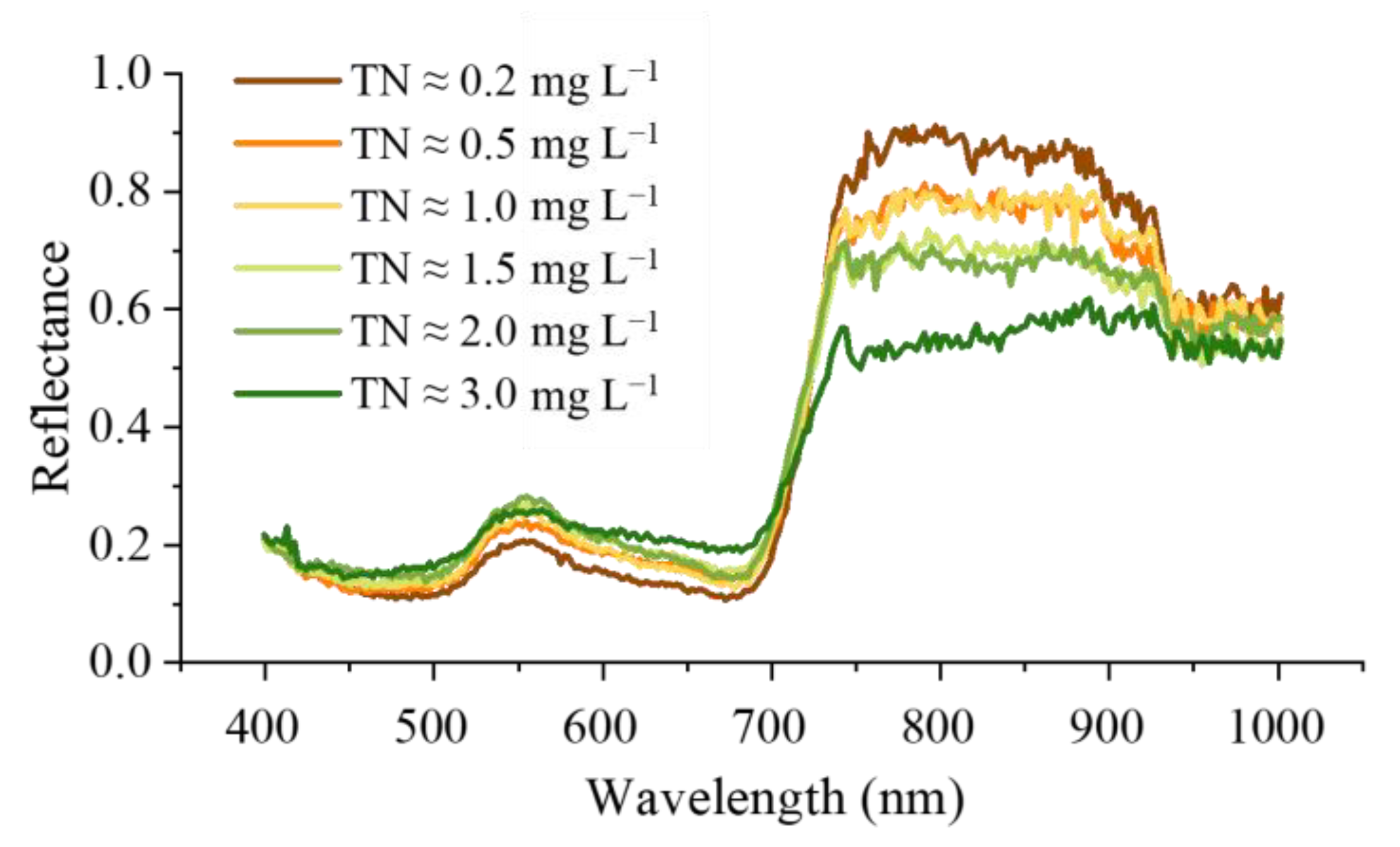
3.2. Average Reflectance and Wavelet Power Spectrum of Emergent Plants

The mean OR reflectance, mean FOD spectrum (1st and 2nd order integers), and mean wavelet power spectrum of 1st order FOD (scales 1–8 (L1~L8)) are shown in Figure 3. The OR has 49 peaks and 50 troughs (Figure 3A1), while the FOD spectrum has 95 peaks and 95 troughs (Figure 3A2). These numbers (peaks and troughs) intuitively reveal that the FOD spectrum contains more detailed information than the OR curve (Figure 3).
Affected by various environments, the OR spectral curve data will contain a lot of noise manifested as many “small burrs” on the spectral curve, which can be visualized in Figure 2. Noise removal is required to reduce the impact of these small burrs. The decomposition and reconstruction process of DWT analysis is carried out iteratively by removing the noise of high-frequency components with filters to finally reconstruct the different signal sub-bands in the spatial domain. Taking the DWT of 1st order FOD as an example, compared with the spectrum of OR/FOD (Figure 3A1–A3), the wavelet power spectrum of FOD (L1~L8) showed more simplified information on the number of peaks and valleys as the decomposition proceeded (Figure 3B1–B9), which intuitively indicated that the high frequency signal was further removed, and the noise transfer phenomenon was becoming weaker. Up to L5 (Figure 3B6), there is relatively little noise, and the reflection peak in the green band and the absorption valley in the red band are evident. By L7 and L8 (Figure 3B8,B9), as the spectral details are continuously removed and the spectral curves gradually smooth out, certain absorption peaks characterizing the correlation between TN and P. australis chlorophyll in water disappear. The OR wavelet power spectra and other FOD wavelet power spectra (L1~L8) exhibit similar behavior, where DWT removes noise while simplifying differences in the spectral bands.

3.3. Correlation Analysis of Preprocessed Spectral and TN Concentration in Water

The correlation coefficients of the preprocessed spectral reflectance and the TN concentration in water are shown in Figure 4. For the OR data, the sensitive spectral wavelengths are mainly concentrated between 400 and 720 nm, while the strongest correlation (0.61) is observed at 690 nm in the OR without DWT treatment. After DWT preprocessing, the FOD results for order 0.1–0.9 exhibit more continuous dark red regions, which better highlight the spectral details and reduce noise. DWT analysis was applied to the FOD spectra with order 0.3–0.8; the red regions from 400–720 nm are extended to 400–800 nm, and the correlation between the spectral reflectance of the extended spectral region (750–800 nm) and the TN concentration of water improves, where the highest correlation (0.80) is found for L8 at 586 nm. The clustering region in the sensitive spectral band is more discrete (especially between 500 and 720 nm) when the FOD order reaches or exceeds 1.0. Nevertheless, the sensitivity of the spectral region from 800–900 nm gradually becomes apparent. The spectral region between 900 and 1000 nm is decomposed and reconstructed, shifting from relatively discrete, negatively correlated spectral reflectance to relatively concentrated, positively correlated spectral reflectance.
For different decomposition layers (L1–L8) of DWT, the correlation coefficients between the spectra of each layer treated with wavelets and the concentration of TN in the water column were improved compared with the spectral information before treatment. The sensitivity of 45% of the OR spectra to TN in water was increased by 0.01–0.22, whereas the correlation between 54% of the FOD spectra and TN was increased by 0.01–0.57.

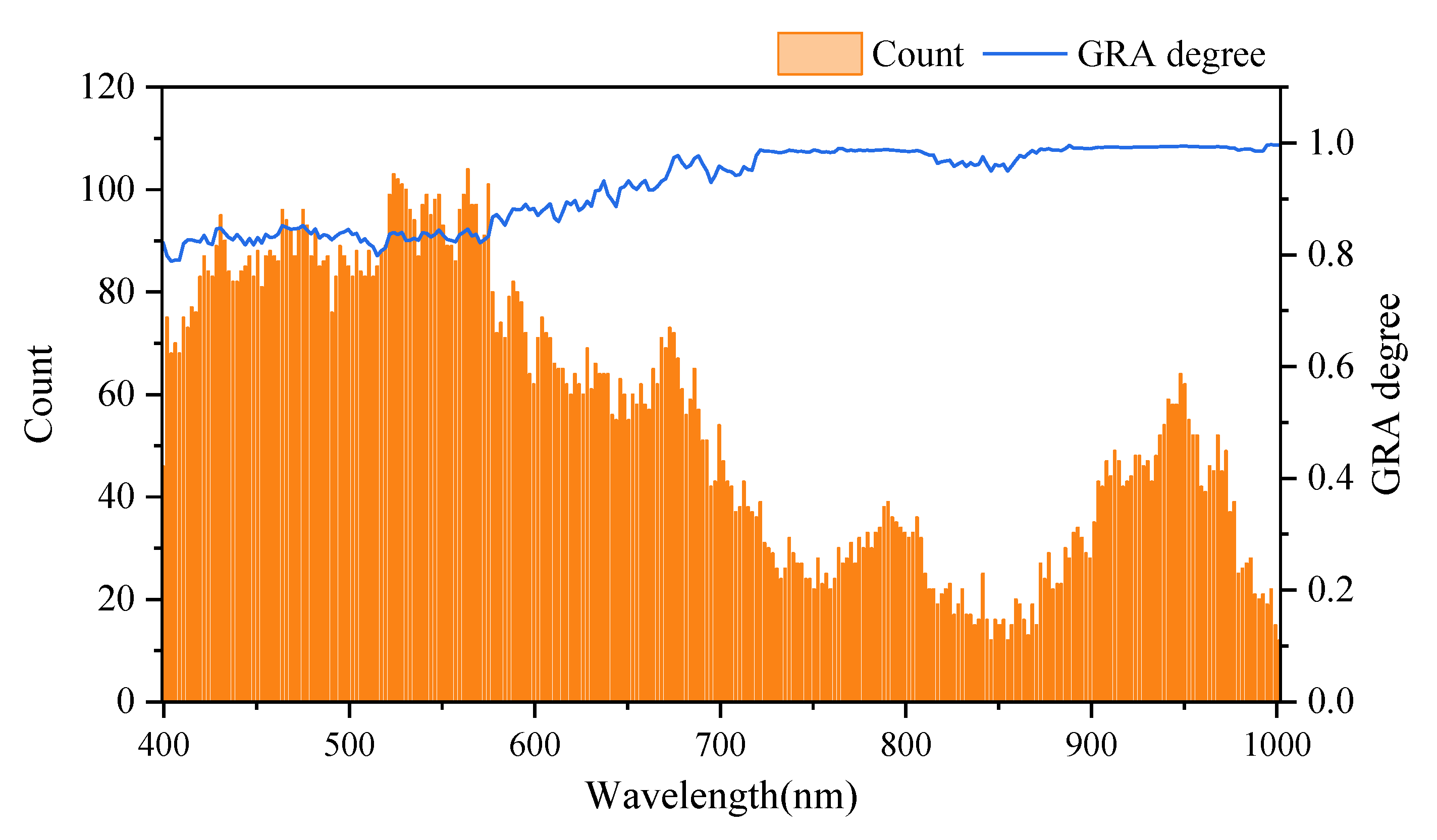
3.4. Grey Relation Analysis

GRA was performed for each layer of the wavelet analysis feature spectra, and all correlation degrees are 0.6 and above. The spectra with a correlation degree of 0.8 or higher and high aggregation between the characteristic spectra of each layer and the TN concentration in water are concentrated in five spectral regions, including 400–420 nm, 440–510 nm, 530–610 nm, 630–710 nm, and 750–830 nm, which indicates that the wavelet analysis could amplify sensitive spectral information while removing noise. For the OR of L1–L8 and the spectral analysis results after FOD transformation, we selected the spectral data with a GRA degree of 0.8 and above (the number distribution is shown in the figure) as the input of the model, and the number distribution (Figure 5) confirms that the spectral region with high sensitivity to the TN concentration in water is between 400 and 700 nm. Overall, the combination of DWT and differential processing techniques not only retains spectral details, but also removes noise.

3.5. Performance of Models Based on Reflectance, Derivative, and Wavelet Power Spectrum

To investigate the strengths of DWT analysis in extracting the TN concentration in water from hyperspectral reflectance data, we summarized and compared the accuracy of 567 models for the OR hyperspectral reflectance, FOD, and wavelet power spectra (Figure 6 and Table 2).
Compared to the OR (Table 2), the model R2 mean values were lower at wavelet scales of L1 to L4 with average model performance ability, while the R2 mean values at scales L5 to L8 indicated a better performance than the OR model, and the best model prediction ability was achieved at L8 (R2 = 0.71, RMSE = 0.62, RPD = 1.74). The same results were obtained for the FOD spectra, where the low-scale (L1) model had average performance. As the decomposition scale increased, the model predictions improved, and the best integrated prediction ability was obtained at L6 (R2 = 0.69, RMSE = 0.44, RPD = 1.78). Overall, the prediction model with the DWT applied has better regression performance than the OR model.
Furthermore, at the eight scales of DWT analysis (Figure 6), the GRA results indicate that the three models follow the order bagging > XGBoost > RF. However, the accuracy values (R2, RMSE, and RPD) of these prediction models do not differ significantly from each other, indicating that the input selection process is objectively accurate. The highest accuracy among the RF models appears in L3 with R2 = 0.86; likewise, the best accuracy of the bagging models appears in L4 with R2 = 0.85. The best-performing model among the XGBoost models appears in L6 with R2 = 0.91.
The regression performance of the different models (RF, bagging, and XGBoost) were assessed based on the wavelet power spectra. Among the 27 models developed for the OR and its DWT hyperspectral data, 12.5% of the RF model accuracy (R2) values are improved by 0.03 compared to the OR model, 87.5% of the bagging model accuracy (R2) values are improved by 0.01–0.27 compared to the OR model, and the XGBoost model shows average performance. Among the 540 models using FOD and DWT with FOD, 82% of the RF model R2 values are improved by 0.02–0.72 compared to the spectral model using FOD, 78.8% of the bagging model R2 values are improved by 0.01–0.53 compared to the spectral model using FOD, and 65.0% of the XGBoost model R2 values are improved by 0.01~0.64.

4. Discussion

4.1. Feasibility of Airborne Hyperspectral Reflectance Extraction of TN in Water

Wetland vegetation characteristics are the expression of adaptation to the water environment and have the function of indicating the water quality of the area. Yu et al. and Liu et al. studied the relationship between vegetation growth characteristics and water elements to confirm that emergent plant characteristics (especially chlorophyll) are the critical reflection of water quality [74,75]. Xing et al. concluded that the nitrogen removal and water purification functions of the typical emergency plant P. australis are due to its high nitrogen and phosphorus requirements during growth [15]. Despite the nitrogen absorption by vegetation growth, nitrification and denitrification remain the major denitrification mechanisms [76]. More than 45% of total nitrogen removal occurs via microbial nitrification and denitrification [77]. The root system of P. australis provides an adhesion interface and a habitat for microorganisms. These microorganisms greatly accelerate the interception of organic matter around the roots and the decomposition of suspended matter under favorable conditions (e.g., higher temperatures and a stable water column), doing so, for example, by breaking down large amounts of high molecular, weight-dissolved organic matter into plant-absorbable substances (especially ammonium nitrogen). The sampling time was July in this study, when the water temperature was high and during the growing season of wetland vegetation in the area, providing a hotbed for microbial metabolic action. In addition, P. australis, a wetland plant, is widely distributed and has a well-developed root system with strong enrichment capacity, whose combined action with microorganisms can better absorb TN elements in the water body. Chlorophyll in vegetation characteristics not only indicates the abundance of TN in water, but also is a significant factor affecting the spectral characteristics of vegetation. The study by Li et al. indicated that the chlorophyll concentration of plants is closely related to the TN supply in water [78]. This also provides a reasonable reference for this study to obtain water quality parameters using the vegetation characteristics profile.
Hyperspectral reflectance of airborne emergent vegetation is a comprehensive expression of the various ecological and environmental factors contained in emergent vegetation and a means of indirectly extracting essential information based on the radiant/scattered energy of the target feature [79]. The estimation of hyperspectral reflectance for surface water composition is attributed to the superior sensitivity of TN concentration to hyperspectral reflectance characteristics of specific wavelength spectra. As chlorophyll concentration increases, plant photosynthetically active radiation (PAR) becomes intense and green band reflectance decreases [80]. Sun et al. applied plant spectra to the diagnosis of TN concentration in water and obtained better estimation results, which verified that hyperspectral reflectance data from aquatic plant canopies are workable in monitoring water composition information [23]. In this study, the reflectance of plants decreased with increasing TN concentration levels (Figure 3). Because there are clear spectral mechanisms [81,82,83] to support us in this operation, this paper is reliable for monitoring water quality based on airborne hyperspectral reflectance. In addition, TN concentration inversion results can be improved by airborne hyperspectral reflectance denoising and other processing methods. Notably, the selection of representative training and validation sets in conjunction with the GRA method is also important to produce reliable algorithm results.

4.2. Prerequisites for Accurate Estimation

The hyperspectral reflectance of the canopy contains redundancy. Hence, the db4 mother wavelet function was employed in decomposition and reconstruction on a binary scale to remove noise [84,85,86]. The db4 mother wavelet function decomposes the hyperspectral reflectance into feature spectra of different sub-bands, where each layer characterizes specific details of the original signal; the reconstructed spectra emphasize the relevant dominant signals and attenuate or filter minor signals [87]. Many works have reported DWT processing of hyperspectral data and the consequent identification of key target features with medium-scale decomposition reconstruction [47]. The present study obtained optimal results at L6 (R2 = 0.91, Figure 6), which is consistent with the medium scale mentioned above.
Notably (Table 2), poor predictions were observed at lower scales, both in the OR decomposition layer (L2, R2 = 0.50) and in the FOD (L1, R2 = 0.58). This poor predictive ability probably lies in the fact that noise still exists in the spectrum after wavelet first-layer decomposition and reconstruction, which is not sensitive to the spectral absorption characteristics of the internal structure of P. australis leaves [88]. The results of DWT analysis of hyperspectral data at low scales studied by Cai were also unsatisfactory, and they pointed out the poor denoising ability at low scales and the reduced interpretation ability at high scales [87]. Therefore, the optimal scale is still under the medium scale. In this study, the same problem occurs at the high scale (L7–L8), and its interpretation ability decreases.
The combinations of OR with DWT and FOD with DWT both strengthen the difference of spectral bands with increasing scale to improve model prediction accuracy (Table 2), indicating that the higher the scale is, the more prominently it reflects the effective information of leaf reflection spectra. However, in the decomposition layer at scales of up to L7 (Figure 3B8), the wave peak and trough features progressively disappear from the spectra with the continuous stripping of high-frequency signals, resulting in a decrease in information in the P. australis canopy reflection spectra. Existing studies stated that the spectral information interpretation ability was insufficient at both low and over decomposition scales [89] and the optimum scale of DWT at low scales required further study. In Table 2, the mean performance of some models with FOD is weaker than the results of DWT analysis of the OR at low scales, which seems to be because the FOD amplifies spectral noise while strengthening spectral differences. However, the effective denoising results exhibited by the combination of FOD and DWT provide a new reference method for the processing of UAV airborne hyperspectral data.

4.3. Vegetation Canopy Spectral Response Mechanisms

The researchers concluded that the spectral response regions between the emergency vegetation canopy spectra and TN elements were concentrated in the visible and red-edge regions. Haboudane et al. evaluated N concentrations in winter wheat at different growth stages and found that the 405–418 nm, 670–700 nm, and 761–763 nm regions were sensitive areas for TN [90]. Fava et al. found that the best spectral response region for estimating N concentration involved the long wavelength (740–770 nm) and near infrared (775–820 nm) of the red-edge band [91]. Due to the effect of TN elements, the vegetation reflectance spectral properties were “red-shifted” (630–780 nm) and the reflectance decreased in the red-edge region [92]. Unsurprisingly (Figure 4), the sensitivity of the OR and 0.1–0.9-order FOD after DWT is comparatively strong in the visible region (400–750 nm), as is that of 1st–2nd-order FOD in the near-infrared region (near 950 nm). The internal chlorophyll of plants absorbs the majority of the radiant energy in the visible range [24,93], which is why vegetative spectra can confirm the abundance of various elements in water. When the FOD order reaches or exceeds 1.0, the clustered regions of the sensitive spectral bands become more discrete, and the red-edge band (800–1000 nm) exhibits greater sensitivity. This spectral reflectance feature has a strong correlation with the internal structure of plant leaves (water, protein, chlorophyll, sugar, etc.) [94].
Some insignificant spectral bands are apparent after correlation analysis of the preprocessed spectra (Figure 4). If all discrete wavelet feature spectra are individually considered as independent variables to build the TN inversion model in water, the sensitive bands of certain decomposition layers could be ignored, resulting in the selected sensitive bands not fully explaining the TN in water bodies and limitations of the constructed model [47,95]. In this study, the optimal sensitive bands are selected by GRA as independent variables to build the optimal estimation model of TN in water. We regarded the spectral regions with high relation coefficients and GRA above 0.8 as sensitive bands (Figure 4 and Figure 5). The sensitive bands were focused in mostly four spectral regions, including blue (450 nm), green (550 nm), red (670 nm), and near-infrared regions (950 nm). The results of this study are coherent with the existing research results. In summary, the combination of wavelet transform and GRA can better highlight sensitive band information related to TN concentration.

4.4. The Potential of the Developed Model

Three integrated learning models (RF, XGBoost, and bagging) were employed to predict TN. For all three models, the independent variables are randomly divided into a modeling set (70%, n = 30) and a validation set (30%, n = 15) and fixed by a function, which also ensures the reasonableness of the input samples. Figure 6 shows that all three models exhibited clear explanatory power (RPD mean > 1.5). However, the variation among the modeling results is substantial, and the optimal result was obtained with XGBoost, which can best describe the quantitative relationship between the reflectivity of the sensitive band and TN in water. The modeling accuracy is comparatively balanced for the bagging model; in the RF model based on the reflectance of the sensitive band, higher-sensitivity information is underestimated, although the RF are valid for this nonlinear issue [63,65]. Therefore, the XGBoost model is recommended to explain the relationship between the TN concentration in water and hyperspectral reflectance. The results of this study indicate that the combination of DWT and GRA generally enhances the accuracy of TN estimation in water (Table 2). Considering the difficulty of raw spectral feature extraction, it is recommended that DWT be applied to preprocess spectral reflectance data, especially in hyperspectral applications. A practical approach is provided for airborne hyperspectral data monitoring of water body components.

4.5. Research Challenges

DWT processing of hyperspectral reflectance data is analyzed in detail in this study. However, the wavelet mother function, reconstruction methods and threshold selection rules, wavelet decomposition scale, and other factors affect the denoising effectiveness to some degree; moreover, information decomposed at too high a scale is difficult to interpret. In future work, it will be critical to investigate the selection methods of the above wavelet factors and their combination techniques to further improve the hyperspectral reflectance denoising effect and thus enhance the analysis capability of DWT spectra. We compared the results of the three models and found that DWT combined with GRA produced the best prediction accuracy; however, it was not easy to determine exactly which wavelength range contributed optimally to the TN model of water. The presented inversion model, which is based on the spectral reflectance of the canopy of inland lake wetland vegetation, and the applicability of the model in other regions or in monitoring water bodies dependent on different wetland vegetation warrants further validation. Moreover, the influences of environmental factors (such as surrounding soil properties, leaf biochemical composition, and canopy structure) and complex interactions between substances within the water of water quality information extraction need to be further investigated.

5. Conclusions

The potential of discrete wavelet transform (DWT) combined with grey relation analysis (GRA) and different machine learning approaches for TN monitoring in water was explored using leaf hyperspectral data. The results of this study in hyperspectral data processing and extraction of water quality parameters once again demonstrated that the application of hyperspectral reflectance to water quality remote sensing is effective and provides a new technological approach for global water environmental protection. The following conclusions can be drawn:
(1)
DWT with appropriate scales is an outstanding technique for preprocessing hyperspectral data. The preprocessing method of fractional order discretization (FOD) combined with DWT may provide basic technical support for hyperspectral signal denoising and could enrich the preprocessing methods of UAV or satellite hyperspectral images.
(2)
The hyperspectral information of emergent vegetation can be efficiently used for the estimation of TN in water. This approach offers a novel reference method for hyperspectral reflectance data monitoring and the protection of global inland water quality, serving the goals of water resource protection and water pollution management for sustainable development.
(3)
The XGBoost model shows remarkable explanatory power for the intrinsic relationship between TN in water and the spectrum of aquatic vegetation.
These results may contribute to further mining of airborne hyperspectral data information, which also provides a new reference for accurate water quality monitoring of complex global waters using UAV or satellite hyperspectral data. In the future, we need to further explore both the method of DWT and the influence of the complexity of water and their environment on water quality extraction.

Author Contributions

Conceptualization, J.D. and J.L.; methodology, J.L.; software, J.L.; validation, X.G. and J.L.; formal analysis, J.L.; investigation, X.G. and J.W.; resources, J.D.; data curation, J.W. and X.G.; writing—original draft preparation, J.L.; writing—review and editing, J.L., X.G. and J.W.; supervision, J.D.; project administration, J.D. and J.W.; funding acquisition, J.D. and J.W. All authors have read and agreed to the published version of the manuscript.

Funding

This research was funded by National Natural Science Foundation of China (No. 42171269), Xinjiang Academician Workstation Cooperative Research Project (No. 2020.B-001), the Graduate Student Innovation Project of Xinjiang Uygur Autonomous Region (XJ2021G041), and Guangdong Basic and Applied Basic Research Foundation (2020A1515111142).

Acknowledgments

We express our sincere appreciation to the experts and professors who took the time to review this paper during their busy schedules. The constructive comments and insightful suggestions you provided will significantly help us to improve this manuscript.

Conflicts of Interest

The authors declare no conflict of interest.

References

  1. Gruber, N.; Galloway, J.N. An Earth-system perspective of the global nitrogen cycle. Nature 2008, 451, 293–296. [Google Scholar] [CrossRef]
  2. Varol, M. Use of water quality index and multivariate statistical methods for the evaluation of water quality of a stream affected by multiple stressors: A case study. Environ. Pollut. 2020, 266, 115417. [Google Scholar] [CrossRef]
  3. Yu, C.; Huang, X.; Chen, H.; Godfray, H.C.J.; Wright, J.S.; Hall, J.W.; Gong, P.; Ni, S.; Qiao, S.; Huang, G. Managing nitrogen to restore water quality in China. Nature 2019, 567, 516–520. [Google Scholar] [CrossRef]
  4. Wang, X.; Zhang, F.; Ghulam, A.; Trumbo, A.L.; Yang, J.; Ren, Y.; Jing, Y. Evaluation and estimation of surface water quality in an arid region based on EEM-PARAFAC and 3D fluorescence spectral index: A case study of the Ebinur Lake Watershed, China. Catena 2017, 155, 62–74. [Google Scholar] [CrossRef]
  5. Li, B.; Yang, G.; Wan, R. Multidecadal water quality deterioration in the largest freshwater lake in China (Poyang Lake): Implications on eutrophication management. Environ. Pollut. 2020, 260, 114033. [Google Scholar] [CrossRef] [PubMed]
  6. Nam, G.; Shin, H.; Ha, R.; Song, H.; Yoo, J.; Lee, H.; Park, S.; Kang, T.; Kim, K. Quantification of Phycocyanin in Inland Waters through Remote Measurement of Ratios and Shifts in Reflection Spectral Peaks. Remote Sens. 2021, 13, 3335. [Google Scholar] [CrossRef]
  7. Galloway, J.N. The global nitrogen cycle: Changes and consequences. Environ. Pollut. 1998, 102, 15–24. [Google Scholar] [CrossRef]
  8. Sagan, V.; Peterson, K.T.; Maimaitijiang, M.; Sidike, P.; Sloan, J.; Greeling, B.A.; Maalouf, S.; Adams, C. Monitoring inland water quality using remote sensing: Potential and limitations of spectral indices, bio-optical simulations, machine learning, and cloud computing. Earth-Sci. Rev. 2020, 205, 103187. [Google Scholar] [CrossRef]
  9. Erisman, J.W.; Galloway, J.N.; Seitzinger, S.; Bleeker, A.; Dise, N.B.; Petrescu, A.M.R.; Leach, A.M.; de Vries, W. Consequences of human modification of the global nitrogen cycle. Philos. Trans. R. Soc. B Biol. Sci. 2013, 368, 0962–8436. [Google Scholar] [CrossRef] [PubMed] [Green Version]
  10. Niu, C.; Tan, K.; Jia, X.; Wang, X. Deep learning based regression for optically inactive inland water quality parameter estimation using airborne hyperspectral imagery. Environ. Pollut. 2021, 286, 117534. [Google Scholar] [CrossRef]
  11. Gómez, D.; Salvador, P.; Sanz, J.; Casanova, J.L. A new approach to monitor water quality in the Menor sea (Spain) using satellite data and machine learning methods. Environ. Pollut. 2021, 286, 117489. [Google Scholar] [CrossRef]
  12. Dechant, B.; Cuntz, M.; Vohland, M.; Schulz, E.; Doktor, D. Estimation of photosynthesis traits from leaf reflectance spectra: Correlation to nitrogen content as the dominant mechanism. Remote Sens. Environ. 2017, 196, 279–292. [Google Scholar] [CrossRef]
  13. Fan, S.; Liu, H.; Zheng, G.; Wang, Y.; Wang, S.; Liu, Y.; Liu, X.; Wan, Y. Differences in phytoaccumulation of organic pollutants in freshwater submerged and emergent plants. Environ. Pollut. 2018, 241, 247–253. [Google Scholar] [CrossRef] [PubMed]
  14. Cui, L.; Dou, Z.; Liu, Z.; Zuo, X.; Lei, Y.; Li, J.; Zhao, X.; Zhai, X.; Pan, X.; Li, W. Hyperspectral Inversion of Phragmites Communis Carbon, Nitrogen, and Phosphorus Stoichiometry Using Three Models. Remote Sens. 2020, 12, 1998. [Google Scholar] [CrossRef]
  15. Xing, W.; Han, Y.; Guo, Z.; Zhou, Y. Quantitative study on redistribution of nitrogen and phosphorus by wetland plants under different water quality conditions. Environ. Pollut. 2020, 261, 114086. [Google Scholar] [CrossRef] [PubMed]
  16. Ke, L.; Xinming, T.; Wenji, Z.; Bing, L.; Xiaoyu, G.; Zhaoning, G. Study on Relationship Between Nitrogen Nutrients in Water and Hyperspectral Characteristics of Wetland Plants. Geogr. Geo-Inf. Sci. 2015, 031, 24–28. [Google Scholar]
  17. Białowiec, A.; Janczukowicz, W.; Randerson, P.F. Nitrogen removal from wastewater in vertical flow constructed wetlands containing LWA/gravel layers and reed vegetation. Ecol. Eng. 2011, 37, 897–902. [Google Scholar] [CrossRef]
  18. Krekov, G.M.; Krekova, M.M.; Lisenko, A.A.; Sukhanov, A.Y. Radiative characteristics of plant leaf. Atmos. Ocean. Opt. 2009, 22, 241–256. [Google Scholar] [CrossRef]
  19. Asner, G.P. Biophysical and biochemical sources of variability in canopy reflectance. Remote Sens. Environ. 1998, 64, 234–253. [Google Scholar] [CrossRef]
  20. El-Hendawy, S.; Al-Suhaibani, N.; Elsayed, S.; Refay, Y.; Alotaibi, M.; Dewir, Y.H.; Hassan, W.; Schmidhalter, U. Combining biophysical parameters, spectral indices and multivariate hyperspectral models for estimating yield and water productivity of spring wheat across different agronomic practices. PLoS ONE 2019, 14, e0212294. [Google Scholar]
  21. Hansen, P.M.; Schjoerring, J.K. Reflectance measurement of canopy biomass and nitrogen status in wheat crops using normalized difference vegetation indices and partial least squares regression. Remote Sens. Environ. 2003, 86, 542–553. [Google Scholar] [CrossRef]
  22. Cho, M.A.; Skidmore, A.K. A new technique for extracting the red edge position from hyperspectral data: The linear extrapolation method. Remote Sens. Environ. 2006, 101, 181–193. [Google Scholar] [CrossRef]
  23. Sun, X.; Zhang, Y.; Shi, K.; Zhang, Y.; Li, N.; Wang, W.; Huang, X.; Qin, B. Monitoring water quality using proximal remote sensing technology. Sci. Total Environ. 2022, 803, 149805. [Google Scholar] [CrossRef] [PubMed]
  24. Li, W.; Dou, Z.; Cui, L.; Wang, R.; Zhao, Z.; Cui, S.; Lei, Y.; Li, J.; Zhao, X.; Zhai, X. Suitability of hyperspectral data for monitoring nitrogen and phosphorus content in constructed wetlands. Remote Sens. Lett. 2020, 11, 495–504. [Google Scholar] [CrossRef]
  25. Guo, M.; Li, J.; Sheng, C.; Xu, J.; Wu, L. A review of wetland remote sensing. Sensors 2017, 17, 777. [Google Scholar] [CrossRef] [PubMed] [Green Version]
  26. Zeng, C.; Richardson, M.; King, D.J. The impacts of environmental variables on water reflectance measured using a lightweight unmanned aerial vehicle (UAV)-based spectrometer system. ISPRS J. Photogramm. Remote Sens. 2017, 130, 217–230. [Google Scholar] [CrossRef]
  27. Jiang, Q.; Xu, L.; Sun, S.; Wang, M.; Xiao, H. Retrieval model for total nitrogen concentration based on UAV hyper spectral remote sensing data and machine learning algorithms—A case study in the Miyun Reservoir, China. Ecol. Indic. 2021, 124, 107356. [Google Scholar] [CrossRef]
  28. Su, T.-C.; Chou, H.-T. Application of multispectral sensors carried on unmanned aerial vehicle (UAV) to trophic state mapping of small reservoirs: A case study of Tain-Pu reservoir in Kinmen, Taiwan. Remote Sens. 2015, 7, 10078–10097. [Google Scholar] [CrossRef] [Green Version]
  29. Cillero Castro, C.; Domínguez Gómez, J.A.; Delgado Martín, J.; Hinojo Sánchez, B.A.; Cereijo Arango, J.L.; Cheda Tuya, F.A.; Díaz-Varela, R. An UAV and satellite multispectral data approach to monitor water quality in small reservoirs. Remote Sens. 2020, 12, 1514. [Google Scholar] [CrossRef]
  30. Sonobe, R.; Yamashita, H.; Mihara, H.; Morita, A.; Ikka, T. Hyperspectral reflectance sensing for quantifying leaf chlorophyll content in wasabi leaves using spectral pre-processing techniques and machine learning algorithms. Int. J. Remote Sens. 2021, 42, 1311–1329. [Google Scholar] [CrossRef]
  31. Wang, J.; Shi, T.; Yu, D.; Teng, D.; Ge, X.; Zhang, Z.; Yang, X.; Wang, H.; Wu, G. Ensemble machine-learning-based framework for estimating total nitrogen concentration in water using drone-borne hyperspectral imagery of emergent plants: A case study in an arid oasis, NW China. Environ. Pollut. 2020, 266, 115412. [Google Scholar] [CrossRef]
  32. Ge, X.; Wang, J.; Ding, J.; Cao, X.; Zhang, Z.; Liu, J.; Li, X. Combining UAV-based hyperspectral imagery and machine learning algorithms for soil moisture content monitoring. PeerJ 2019, 7, e6926. [Google Scholar] [CrossRef] [PubMed]
  33. Wang, L.W.; Wei, Y.X. Estimating the total nitrogen and total phosphorus content of wetland soils using hyperspectral models. Acta Ecol. Sin. 2016, 36, 5116–5125. [Google Scholar]
  34. Yuan, J.; Zhang, F.; Ge, X.Y.; Guo, W.Z.; Deng, L.F. Leaf salt ion content estimation of halophyte plants based on geographically weighted regression model combined with hyperspectral data. Trans. Chin. Soc. Agric. Eng. 2019, 35, 115–124. [Google Scholar]
  35. Srivastava, P.K.; Malhi, R.K.M.; Pandey, P.C.; Anand, A.; Singh, P.; Pandey, M.K.; Gupta, A. Revisiting hyperspectral remote sensing: Origin, processing, applications and way forward. In Hyperspectral Remote Sensing; Elsevier: Amsterdam, The Netherlands, 2020; pp. 3–21. [Google Scholar]
  36. Ge, X.; Ding, J.; Jin, X.; Wang, J.; Chen, X.; Li, X.; Liu, J.; Xie, B. Estimating Agricultural Soil Moisture Content through UAV-Based Hyperspectral Images in the Arid Region. Remote Sens. 2021, 13, 1562. [Google Scholar] [CrossRef]
  37. Lin, X.; Su, Y.-C.; Shang, J.; Sha, J.; Li, X.; Sun, Y.-Y.; Ji, J.; Jin, B. Geographically Weighted Regression Effects on Soil Zinc Content Hyperspectral Modeling by Applying the Fractional-Order Differential. Remote Sens. 2019, 11, 636. [Google Scholar] [CrossRef] [Green Version]
  38. Liu, D.; Chi, Y. Horizontal and vertical distributions of estuarine soil total organic carbon and total nitrogen under complex land surface characteristics. Glob. Ecol. Conserv. 2020, 24, e01268. [Google Scholar] [CrossRef]
  39. Wang, J.; Hu, X.; Shi, T.; He, L.; Hu, W.; Wu, G. Assessing toxic metal chromium in the soil in coal mining areas via proximal sensing: Prerequisites for land rehabilitation and sustainable development. Geoderma 2022, 405, 115399. [Google Scholar] [CrossRef]
  40. Dabiri, A.; Nazari, M.; Butcher, E.A. The spectral parameter estimation method for parameter identification of linear fractional order systems. In Proceedings of the 2016 American Control Conference (ACC), Boston, MA, USA, 6–8 July 2016; pp. 2772–2777. [Google Scholar]
  41. Bhadra, S.; Sagan, V.; Maimaitijiang, M.; Maimaitiyiming, M.; Newcomb, M.; Shakoor, N.; Mockler, T.C. Quantifying Leaf Chlorophyll Concentration of Sorghum from Hyperspectral Data Using Derivative Calculus and Machine Learning. Remote Sens. 2020, 12, 2082. [Google Scholar] [CrossRef]
  42. Wang, G.; Wang, W.; Fang, Q.; Jiang, H.; Xin, Q.; Xue, B. The Application of Discrete Wavelet Transform with Improved Partial Least-Squares Method for the Estimation of Soil Properties with Visible and Near-Infrared Spectral Data. Remote Sens. 2018, 10, 867. [Google Scholar] [CrossRef] [Green Version]
  43. Bazine, R.; Wu, H.; Boukhechba, K. Spectral DWT Multilevel Decomposition with Spatial Filtering Enhancement Preprocessing-Based Approaches for Hyperspectral Imagery Classification. Remote Sens. 2019, 11, 2906. [Google Scholar] [CrossRef] [Green Version]
  44. Anand, R.; Veni, S.; Aravinth, J. Robust Classification Technique for Hyperspectral Images Based on 3D-Discrete Wavelet Transform. Remote Sens. 2021, 13, 1255. [Google Scholar] [CrossRef]
  45. Peng, J.; Hong, S.; He, S.W.; Wu, J.S. Soil moisture retrieving using hyperspectral data with the application of wavelet analysis. Environ. Earth Sci. 2013, 69, 279–288. [Google Scholar] [CrossRef]
  46. Blackburn, G.A. Wavelet decomposition of hyperspectral data: A novel approach to quantifying pigment concentrations in vegetation. Int. J. Remote Sens. 2007, 28, 2831–2855. [Google Scholar] [CrossRef]
  47. Li, F.; Wang, L.; Liu, J.; Wang, Y.; Chang, Q. Evaluation of leaf N concentration in winter wheat based on discrete wavelet transform analysis. Remote Sens. 2019, 11, 1331. [Google Scholar] [CrossRef] [Green Version]
  48. Meng, X.; Bao, Y.; Liu, J.; Liu, H.; Zhang, X.; Zhang, Y.; Wang, P.; Tang, H.; Kong, F. Regional soil organic carbon prediction model based on a discrete wavelet analysis of hyperspectral satellite data. Int. J. Appl. Earth Obs. Geoinf. 2020, 89, 102111. [Google Scholar] [CrossRef]
  49. Haiwei, Z.; Fei, Z.; Zhe, L.; Yushanjiang, A.; Yun, C. Spectral diagnosis and spatial distribution of SS, TN and TP in surface water in Ebinur Lake Watershed. Ecol. Environ. Sci. 2017, 26, 1042–1050. [Google Scholar]
  50. Osco, L.P.; Ramos, A.P.M.; Faita Pinheiro, M.M.; Moriya, É.A.S.; Imai, N.N.; Estrabis, N.; Ianczyk, F.; Araújo, F.F.d.; Liesenberg, V.; Jorge, L.A.d.C. A Machine Learning Framework to Predict Nutrient Content in Valencia-Orange Leaf Hyperspectral Measurements. Remote Sens. 2020, 12, 906. [Google Scholar] [CrossRef] [Green Version]
  51. Hong, Y.; Liu, Y.; Chen, Y.; Liu, Y.; Yu, L.; Liu, Y.; Cheng, H. Application of fractional-order derivative in the quantitative estimation of soil organic matter content through visible and near-infrared spectroscopy. Geoderma 2019, 337, 758–769. [Google Scholar] [CrossRef]
  52. Zhang, Z.; Ding, J.; Wang, J.; Ge, X. Prediction of soil organic matter in northwestern China using fractional-order derivative spectroscopy and modified normalized difference indices. CATENA 2020, 185, 104257. [Google Scholar] [CrossRef]
  53. Wang, J.; Ding, J.; Abulimiti, A.; Cai, L. Quantitative estimation of soil salinity by means of different modeling methods and visible-near infrared (VIS–NIR) spectroscopy, Ebinur Lake Wetland, Northwest China. PeerJ 2018, 6, e4703. [Google Scholar] [CrossRef] [PubMed] [Green Version]
  54. Bruce, L.M.; Koger, C.H.; Jiang, L. Dimensionality reduction of hyperspectral data using discrete wavelet transform feature extraction. IEEE Trans. Geosci. Remote Sens. 2002, 40, 2331–2338. [Google Scholar] [CrossRef]
  55. Banskota, A.; Wynne, R.H.; Thomas, V.A.; Serbin, S.P.; Kayastha, N.; Gastellu-Etchegorry, J.P.; Townsend, P.A. Investigating the utility of wavelet transforms for inverting a 3-D radiative transfer model using hyperspectral data to retrieve forest LAI. Remote Sens. 2013, 5, 2639–2659. [Google Scholar] [CrossRef]
  56. Starosolski, R. Hybrid Adaptive Lossless Image Compression Based on Discrete Wavelet Transform. Entropy 2020, 22, 751. [Google Scholar] [CrossRef] [PubMed]
  57. Wei, Y.; Ding, J.; Yang, S.; Wang, F.; Wang, C. Soil salinity prediction based on scale-dependent relationships with environmental variables by discrete wavelet transform in the Tarim Basin. Catena 2021, 196, 104939. [Google Scholar] [CrossRef]
  58. Cao, X.; Yao, J.; Fu, X.; Bi, H.; Hong, D. An Enhanced 3-D Discrete Wavelet Transform for Hyperspectral Image Classification. IEEE Geosci. Remote Sens. Lett. 2021, 18, 1104–1108. [Google Scholar] [CrossRef]
  59. AbdelFattah, M.; AbdelAal, L.F.; El-khoribi, R. Spectral-spatial hyperspectral image classification based on randomized singular value decomposition and 3-dimensional discrete wavelet transform. Int. J. Comput. Appl. 2018, 975, 8887. [Google Scholar] [CrossRef]
  60. Shiri, J.; Keshavarzi, A.; Kisi, O.; Karimi, S.M.; Karimi, S.; Nazemi, A.H.; Rodrigo-Comino, J. Estimating Soil Available Phosphorus Content through Coupled Wavelet–Data-Driven Models. Sustainability 2020, 12, 1250. [Google Scholar] [CrossRef] [Green Version]
  61. Cai, L.; Ding, J. Inversion of Soil Moisture Content Based on Hyperspectral Multi-Scale Decomposition. Laser Optoelectron. Prog. 2018, 55, 013001. [Google Scholar]
  62. Wang, J.; Ding, J.; Yu, D.; Ma, X.; Zhang, Z.; Ge, X.; Teng, D.; Li, X.; Liang, J.; Lizaga, I.; et al. Capability of Sentinel-2 MSI data for monitoring and mapping of soil salinity in dry and wet seasons in the Ebinur Lake region, Xinjiang, China. Geoderma 2019, 353, 172–187. [Google Scholar] [CrossRef]
  63. Yang, S.; Hu, L.; Wu, H.; Ren, H.; Fan, W. Integration of crop growth model and random forest for winter wheat yield estimation from UAV hyperspectral imagery. IEEE J. Sel. Top. Appl. Earth Obs. Remote Sens. 2021, 14, 6253–6269. [Google Scholar] [CrossRef]
  64. Siedliska, A.; Baranowski, P.; Pastuszka-Woniak, J.; Zubik, M.; Krzyszczak, J. Identification of plant leaf phosphorus content at different growth stages based on hyperspectral reflectance. BMC Plant Biol. 2021, 21, 1–17. [Google Scholar] [CrossRef] [PubMed]
  65. Parsaie, F.; Firouzi, A.F.; Mousavi, S.R.; Rahmani, A.; Homaee, M. Large-scale digital mapping of topsoil total nitrogen using machine learning models and associated uncertainty map. Environ. Monit. Assess. 2021, 193, 1–15. [Google Scholar] [CrossRef] [PubMed]
  66. Kulmatiski, A.; Forero, L.E. Bagging: A cheaper, faster, non-destructive transpiration water sampling method for tracer studies. Plant Soil 2021, 462, 603–611. [Google Scholar] [CrossRef]
  67. Jia, S.; Jian, Y.; Shi, S.; Chen, B.; Du, L.; Gong, W.; Song, S. Estimating Rice Leaf Nitrogen Concentration: Influence of Regression Algorithms Based on Passive and Active Leaf Reflectance. Remote Sens. 2017, 9, 951. [Google Scholar]
  68. Barradas, A.; Correia, P.; Silva, S.; Mariano, P.; Silva, J.M.D. Comparing Machine Learning Methods for Classifying Plant Drought Stress from Leaf Reflectance Spectra in Arabidopsis thaliana. Appl. Sci. 2021, 11, 6392. [Google Scholar] [CrossRef]
  69. Moghimi, A.; Pourreza, A.; Zuniga-Ramirez, G.; Williams, L.E.; Fidelibus, M.W. A Novel Machine Learning Approach to Estimate Grapevine Leaf Nitrogen Concentration Using Aerial Multispectral Imagery. Remote Sens. 2020, 12, 3515. [Google Scholar] [CrossRef]
  70. Iatrou, M.; Karydas, C.; Iatrou, G.; Pitsiorlas, I.; Mourelatos, S. Topdressing Nitrogen Demand Prediction in Rice Crop Using Machine Learning Systems. Agriculture 2021, 11, 312. [Google Scholar] [CrossRef]
  71. Andrade, R.; Silva, S.; Weindorf, D.C.; Chakraborty, S.; Curi, N. Assessing models for prediction of some soil chemical properties from portable X-ray fluorescence (pXRF) spectrometry data in Brazilian Coastal Plains. Geoderma 2020, 357, 113957. [Google Scholar] [CrossRef]
  72. Ma, G.; Ding, J.; Han, L.; Zhang, Z.; Ran, S. Digital mapping of soil salinization based on Sentinel-1 and Sentinel-2 data combined with machine learning algorithms. Reg. Sustain. 2021, 2, 177–188. [Google Scholar] [CrossRef]
  73. Xu, X.; Chen, S.; Ren, L.; Han, C.; Lv, D.; Zhang, Y.; Ai, F. Estimation of Heavy Metals in Agricultural Soils Using Vis-NIR Spectroscopy with Fractional-Order Derivative and Generalized Regression Neural Network. Remote Sens. 2021, 13, 2718. [Google Scholar] [CrossRef]
  74. Yu, H.; Qi, W.; Liu, C.; Yang, L.; Wang, L.; Lv, T.; Peng, J. Different Stages of Aquatic Vegetation Succession Driven by Environmental Disturbance in the Last 38 Years. Water 2019, 11, 1412. [Google Scholar] [CrossRef] [Green Version]
  75. Liu, H.; Liu, G.; Xing, W. Functional traits of submerged macrophytes in eutrophic shallow lakes affect their ecological functions. Sci. Total Environ. 2021, 760, 143332. [Google Scholar] [CrossRef] [PubMed]
  76. Ko, C.-H.; Lee, T.-M.; Chang, F.-C.; Liao, S.-P. The correlations between system treatment efficiencies and aboveground emergent macrophyte nutrient removal for the Hsin-Hai Bridge phase II constructed wetland. Bioresour. Technol. 2011, 102, 5431–5437. [Google Scholar] [CrossRef] [PubMed]
  77. Luederitz, V.; Eckert, E.; Lange-Weber, M.; Lange, A.; Gersberg, R.M. Nutrient removal efficiency and resource economics of vertical flow and horizontal flow constructed wetlands. Ecol. Eng. 2001, 18, 157–171. [Google Scholar] [CrossRef]
  78. Li, H.; Zhao, C.; Yang, G.; Feng, H. Variations in crop variables within wheat canopies and responses of canopy spectral characteristics and derived vegetation indices to different vertical leaf layers and spikes. Remote Sens. Environ. 2015, 169, 358–374. [Google Scholar] [CrossRef]
  79. Austin, Å.N.; Hansen, J.P.; Donadi, S.; Eklöf, J.S. Relationships between aquatic vegetation and water turbidity: A field survey across seasons and spatial scales. PLoS ONE 2017, 12, e0181419. [Google Scholar] [CrossRef] [Green Version]
  80. Li, Y.; Wang, X.; Zhao, Z.; Han, S.; Liu, Z. Lagoon water quality monitoring based on digital image analysis and machine learning estimators. Water Res. 2020, 172, 115471. [Google Scholar] [CrossRef]
  81. Siciliano, D.; Wasson, K.; Potts, D.C.; Olsen, R.C. Evaluating hyperspectral imaging of wetland vegetation as a tool for detecting estuarine nutrient enrichment. Remote Sens. Environ. 2008, 112, 4020–4033. [Google Scholar] [CrossRef] [Green Version]
  82. Berger, K.; Verrelst, J.; Féret, J.-B.; Wang, Z.; Wocher, M.; Strathmann, M.; Danner, M.; Mauser, W.; Hank, T. Crop nitrogen monitoring: Recent progress and principal developments in the context of imaging spectroscopy missions. Remote Sens. Environ. 2020, 242, 111758. [Google Scholar] [CrossRef]
  83. Sarigai; Yang, J.; Zhou, A.; Han, L.; Li, Y.; Xie, Y. Monitoring urban black-odorous water by using hyperspectral data and machine learning. Environ. Pollut. 2021, 269, 116166. [Google Scholar] [CrossRef]
  84. Liu, Z.; Zhao, L.; Peng, Y.; Wang, G.; Hu, Y. Improving Estimation of Soil Moisture Content Using a Modified Soil Thermal Inertia Model. Remote Sens. 2020, 12, 1719. [Google Scholar] [CrossRef]
  85. Meng, X.; Bao, Y.; Ye, Q.; Liu, H.; Zhang, X.; Tang, H.; Zhang, X. Soil Organic Matter Prediction Model with Satellite Hyperspectral Image Based on Optimized Denoising Method. Remote Sens. 2021, 13, 2273. [Google Scholar] [CrossRef]
  86. S Sahadevan, A.; Shrivastava, P.; Das, B.S.; Sarathjith, M.C. Discrete Wavelet Transform Approach for the Estimation of Crop Residue Mass From Spectral Reflectance. IEEE J. Sel. Top. Appl. Earth Obs. Remote Sens. 2014, 7, 2490–2495. [Google Scholar] [CrossRef]
  87. Cai, L.; Ding, J. Wavelet transformation coupled with CARS algorithm improving prediction accuracy of soil moisture content based on hyperspectral reflectance. Trans. Chin. Soc. Agric. Eng. 2017, 33, 144–151. [Google Scholar]
  88. Luo, J.; Ma, R.; Feng, H.; Li, X. Estimating the total nitrogen concentration of reed canopy with hyperspectral measurements considering a non-uniform vertical nitrogen distribution. Remote Sens. 2016, 8, 789. [Google Scholar] [CrossRef] [Green Version]
  89. Stratoulias, D.; Balzter, H.; Zlinszky, A.; Tóth, V.R. Assessment of ecophysiology of lake shore reed vegetation based on chlorophyll fluorescence, field spectroscopy and hyperspectral airborne imagery. Remote Sens. Environ. 2015, 157, 72–84. [Google Scholar] [CrossRef] [Green Version]
  90. Haboudane, D.; Tremblay, N.; Miller, J.R.; Vigneault, P. Remote Estimation of Crop Chlorophyll Content Using Spectral Indices Derived From Hyperspectral Data. IEEE Trans. Geosci. Remote Sens. 2008, 46, 423–437. [Google Scholar] [CrossRef]
  91. Fava, F.; Colombo, R.; Bocchi, S.; Meroni, M.; Sitzia, M.; Fois, N.; Zucca, C. Identification of hyperspectral vegetation indices for Mediterranean pasture characterization. Int. J. Appl. Earth Obs. Geoinf. 2009, 11, 233–243. [Google Scholar] [CrossRef]
  92. Stroppiana, D.; Boschetti, M.; Brivio, P.A.; Bocchi, S. Plant nitrogen concentration in paddy rice from field canopy hyperspectral radiometry. Field Crops Res. 2009, 111, 119–129. [Google Scholar] [CrossRef]
  93. Hui, L.I.U.; Zhao ning, G.; Wen ji, Z. Estimating total nitrogen content in reclaimed water based on hyperspectral reflectance information from emergent plants: A case study of Mencheng Lake Wetland Park in Beijing China. Yingyong Shengtai Xuebao 2014, 25, 12. [Google Scholar]
  94. Osco, L.P.; Junior, J.M.; Ramos, A.P.M.; Furuya, D.E.G.; Santana, D.C.; Teodoro, L.P.R.; Gonçalves, W.N.; Baio, F.H.R.; Pistori, H.; Junior, C.A.d.S. Leaf nitrogen concentration and plant height prediction for maize using UAV-based multispectral imagery and machine learning techniques. Remote Sens. 2020, 12, 3237. [Google Scholar] [CrossRef]
  95. Zhang, Y.; Hui, J.; Qin, Q.; Sun, Y.; Zhang, T.; Sun, H.; Li, M. Transfer-learning-based approach for leaf chlorophyll content estimation of winter wheat from hyperspectral data. Remote Sens. Environ. 2021, 267, 112724. [Google Scholar] [CrossRef]
Figure 1. Map of the study area and sampling areas (A) Xinjiang Uyghur Autonomous Region map and (B) Ebinur Lake Wetland National Nature Reserve.
Remotesensing 13 04643 g001
Figure 2. Spectral reflectance curves of P. australis with different TN concentrations (400–1000 nm).
Remotesensing 13 04643 g002
Figure 3. Pretreated spectral reflectance curves. (A1) Mean OR reflectance, (A2,B1) Mean 1st-order FOD spectrum, (A3) Mean 2nd-order FOD spectrum, and (B2B9) Mean wavelet power spectrum of 1st order FOD (scales 1–8 (L1~L8).
Remotesensing 13 04643 g003
Figure 4. Correlation coefficients between TN concentration in water and OR reflectance or pretreated spectral reflectance in the 400–1000 nm spectral region. Positive red and blue green in the graph represent high correlations. The OR range from bottom to top indicates the correlation coefficient between the TN concentration in water and the OR and the wavelet power spectrum at 8 scales of DWT (L1–L8); the same is true for the FOD (0.1–2) range.
Remotesensing 13 04643 g004
Figure 5. Spectral distribution and correlation values of the model input data selected for GRA.
Remotesensing 13 04643 g005
Figure 6. R2 (A), RMSE (B), and RPD (C) box plots for 567 models using RF, Bagging, and XGBoost.
Remotesensing 13 04643 g006
Table 1. Descriptive statistics of TN content in water for the whole, calibration, and validation data sets (mg L−1).
CategoryNMinMaxMeanSDCV
Whole dataset450.123.081.370.850.62
Calibration dataset300.232.651.450.900.62
Validation dataset150.123.081.330.840.63
N is the number of samples, SD is the standard deviation, and CV is coefficient of variation.
Table 2. R2, RMSE, and RPD based on the OR, FOD, and wavelet power spectrum models.
SpectraNumber of ModelsR2RMSERPD
MinMaxMeanSDMinMaxMeanSDMinMaxMeanSD
OR30.530.820.680.140.370.590.460.111.322.131.680.41
OR-130.520.740.620.110.420.570.490.071.381.871.600.25
OR-230.400.630.500.120.400.490.440.051.471.811.610.17
OR-330.620.690.660.040.580.610.590.011.291.671.410.21
OR-430.510.690.600.090.500.610.550.061.451.601.540.08
OR-530.620.790.690.090.480.630.530.091.541.951.800.23
OR-630.620.720.680.050.500.560.540.031.401.911.610.26
OR-730.640.710.680.040.470.500.480.021.642.011.830.18
OR-830.690.720.710.020.570.680.620.061.292.121.740.44
FOD600.140.820.520.140.340.720.540.091.082.271.430.25
FOD-1600.320.840.580.120.390.710.520.071.092.011.490.21
FOD-2600.260.850.620.130.360.720.490.081.082.161.590.24
FOD-3600.380.870.670.110.280.650.460.081.202.741.680.31
FOD-4600.360.860.630.110.330.670.490.071.172.351.600.25
FOD-5600.440.830.690.090.360.660.470.061.182.161.670.21
FOD-6600.420.910.690.110.240.650.44 0.091.203.181.780.40
FOD-7600.520.820.680.070.340.570.450.051.362.261.710.20
FOD-8600.400.850.640.090.320.630.480.061.242.451.630.20
Sum567
OR and FOD are the original reflection spectra and fractional order derivative spectra, respectively, and OR_scale and FOD_scale (L = 1, 2, 3, 4, 5, 6, 7, 8) represent the wavelet power spectra of OR and FOD at specific scales, respectively. SD is the standard deviation.
Publisher’s Note: MDPI stays neutral with regard to jurisdictional claims in published maps and institutional affiliations.

