Article

Improving the Spatial Resolution of GRACE-Derived Terrestrial Water Storage Changes in Small Areas Using the Machine Learning Spatial Downscaling Method

1
School of Aerospace Science and Technology, Xidian University, Xi’an 710126, China
2
Qian Xuesen Laboratory of Space Technology, China Academy of Space Technology, Beijing 100094, China
3
School of Geomatics, Liaoning Technical University, Fuxin 123000, China
4
School of Surveying and Landing Information Engineering, Henan Polytechnic University, Jiaozuo 454000, China
5
School of Electronics and Information Engineering, Harbin Institute of Technology, Harbin 150001, China
6
Tianjin Centre, China Geological Survey, Tianjin 300170, China
*
Author to whom correspondence should be addressed.
Those authors contributed equally to this paper.
Remote Sens. 2021, 13(23), 4760; https://doi.org/10.3390/rs13234760
Submission received: 25 October 2021 / Revised: 16 November 2021 / Accepted: 22 November 2021 / Published: 24 November 2021

Abstract

:
Gravity Recovery and Climate Experiment (GRACE) satellites can effectively monitor terrestrial water storage (TWS) changes in large-scale areas. However, due to the coarse resolution of GRACE products, there is still a large number of deficiencies that need to be considered when investigating TWS changes in small-scale areas. Hence, it is necessary to downscale the GRACE products with a coarse resolution. First, in order to solve this problem, the present study employs modeling windows of different sizes (Window Size, WS) combined with multiple machine learning algorithms to develop a new machine learning spatial downscaling method (MLSDM) in the spatial dimension. Second, The MLSDM is used to improve the spatial resolution of GRACE observations from 0.5° to 0.25°, which is applied to Guantao County. The present study has verified the downscaling accuracy of the model developed through the combination of WS3, WS5, WS7, and WS9 and jointed with Random Forest (RF), Extra Tree Regressor (ETR), Adaptive Boosting Regressor (ABR), and Gradient Boosting Regressor (GBR) algorithms. The analysis shows that the accuracy of each combined model is improved after adding the residuals to the high-resolution downscaled results. In each modeling window, the accuracy of RF is better than that of ETR, ABR, and GBR. Additionally, compared to the changes in the TWS time series that are derived by the model before and after downscaling, the results indicate that the downscaling accuracy of WS5 is slightly more superior compared to that of WS3, WS7, and WS9. Third, the spatial resolution of the GRACE data was increased from 0.5° to 0.05° by integrating the WS5 and RF algorithm. The results are as follows: (1) The TWS (GWS) changes before and after downscaling are consistent, decreasing at −20.86 mm/yr and −21.79 mm/yr (−14.53 mm/yr and −15.46 mm/yr), respectively, and the Nash–Sutcliffe efficiency coefficient (NSE) and correlation coefficient (CC) values of both are above 0.99 (0.98). (2) The CC between the 80% deep groundwater well data and the downscaled GWS changes are above 0.70. Overall, the MLSDM can not only effectively improve the spatial resolution of GRACE products but also can preserve the spatial distribution of the original signal, which can provide a reference scheme for research focusing on the downscaling of GRACE products.

Graphical Abstract

1. Introduction

Water resources are some of the most indispensable material resources for human survival and social development. As the main component of freshwater resources, groundwater is essential for industrial production, agricultural irrigation, and domestic water [1,2]. Affected by climate change, groundwater overexploitation, and lack of effective replenishment, groundwater has been severely depleted in many regions [3,4,5]. Therefore, an accurate estimation of groundwater storage (GWS) changes is necessary for the effective management of water resources and to be able to ensure food security. In particular, irregular changes in factors such as the global surface temperature, rainfall, and evapotranspiration affect water storage balance, leading to droughts, floods, and other disasters [6,7]. This requires some reliable methods that can be used to monitor changes in terrestrial water storage (TWS) and GWS. However, it takes a lot of manpower and material resources to monitor GWS changes through traditional methods such as large-scale monitoring networks. In addition, the use of sparsely and unevenly distributed groundwater observation wells makes it difficult to continuously estimate GWS changes in large-scale areas [8]. Hence, many attempts have been made to improve the spatiotemporal characteristics of GWS changes in recent years, such as hydrological models and satellite remote sensing.
The GRACE satellite, which was successfully launched in 2002, provides an unprecedented approach for the time-continuous, large-scale regional monitoring of TWS changes [9]. Previous studies have demonstrated that GRACE observations can estimate mass changes with an accuracy of 1 to 1.5 cm equivalent water height (EWH) over large-scale areas (~20,000 km2) [10,11,12]. At present, GRACE products have important applications in the study of global TWS changes [13,14], droughts and floods [15,16], glacier melting [17,18], and so on. GRACE-derived TWS changes contain different water storage components, e.g., soil moisture, groundwater, snow mass, and canopy water. According to the water storage balance equation, the corresponding components are subtracted from the TWS to estimate regional GWS changes [19,20]. Through the integration of hydrological simulations, the GRACE satellites have been widely used to analyze the TWS and GWS changes in large-scale areas, such as the Amazon basin [21,22], the Yangtze River basin [23,24], northwestern India [25,26,27], the North China Plain [4,28,29], and California’s Central Valley [5,30,31,32]. Nevertheless, it is challenging to employ GRACE data to profoundly investigate TWS changes in small-scale areas due to the coarse image resolution. Therefore, it is essential to obtain high-resolution GRACE data to analyze changes in terrestrial water and groundwater storage in small-scale areas.
At present, the downscaling of coarse-resolution products is an effective approach that can be used to obtain high-resolution products and mainly include dynamical and statistical downscaling [33,34]. The computational process of dynamical downscaling is complicated and requires extensive computation times and resources [35]. Therefore, it is difficult to implement under normal working conditions, limiting the promotion of this method. Correspondingly, the statistical downscaling method establishes regression models between low-resolution target data and variable data and then inputs high-resolution variable data into the regression model to output high-resolution target data [36]. The statistical downscaling method is easy to implement, and the downscaled results can satisfy the accuracy requirements. Therefore, this method has been widely used to obtain high-resolution hydrological and climate data, such as those pertaining to soil moisture [37,38,39], precipitation [40,41,42], temperature [40,43], and evapotranspiration [44,45].
Many studies attempting to obtain high-resolution GRACE data based on statistical downscaling methods have been conducted. Several earlier studies downscaled GRACE data in different regions through empirical regression relationships and achieved reasonable performance [46,47,48]. For example, Ning et al. (2014) improved the spatial resolution of GRCAE products in Yunnan Province to 0.25° through the statistical regression downscaling method [47]. Specifically, because machine learning algorithms can solve nonlinear regression problems and can simulate complex hydrological processes, these methods are widely utilized in GRACE data downscaling research. For instance, Miro et al. (2018) estimated high-resolution GWS changes from the groundwater basins in the San Joaquin Valley in California using an artificial neural network (ANN) [49]. Seyoum et al. (2019) trained a Boosted Regression Tree (BRT) model to estimate groundwater storage anomalies (GWSA) in a ~150,000 km2 Glacial Aquifer System in the state of Illinois based on terrestrial water storage anomalies (TWSA) and other land surface and hydro-climatic variables [50]. Milewski et al. (2019) downscaled GRACE TWSA products based on the BRT algorithm and obtained groundwater level anomaly maps at a 5 km resolution over the Upper Floridan Aquifer in Georgia [51]. Sahour et al. (2020) introduced three machine learning algorithms to downscale TWSA across the Lower Peninsula of Michigan from a coarse-scale (13,700–33,100 km2) resolution to a fine-scale (0.125° × 0.125° or 120 km2) resolution [52].
Currently, several studies have established downscaling models in terms of temporal dimensions, which are mainly used to analyze large-scale regional TWS changes. However, few studies have established downscaling models in spatial dimensions and applied them to analyze TWS changes in small-scale regions. Unlike previous studies, the new machine learning spatial downscaling method (MLSDM) proposes the cross-combining of multiple machine learning algorithms with differently sized modeling windows in spatial dimensions; the algorithm and the size of the modeling windows are optimized according to the training results. Moreover, this study analyzes the consistency of TWS changes before and after downscaling using root mean square error (RMSE), mean absolute error (MAE), the Nash–Sutcliffe efficiency coefficient (NSE), and the correlation coefficient (CC). Finally, the in situ groundwater well observations are used to analyze the reliability of the downscaled GWSA, providing a certain reference basis for regional groundwater management.

2. The MLSDM for Spatial Downscaling

Generally, a great deal of research focusing on GRACE data downscaling aim to establish the downscaling models of each grid in the temporal dimension (Equation (1)). First, this method establishes the regression relationship between the TWSA and hydrological variables in a specific grid (such as the red grid) (Figure 1a). Then, it gradually establishes the downscaling models of all of the grids through iteration. In this method, the signals that are produced before and after downscaling have good consistency in the spatial distribution. Still, the downscaled signal has a relatively obvious boundary between the grids and does not conform to the characteristics of continuously changing hydrological signals. Hence, some studies have tried to establish downscaling models for GRACE data in the spatial dimension. Figure 1b shows that this method first establishes the regression relationship between the TWSA and hydrological variables in a specific month (such as M1) (Equation (1)). It gradually establishes downscaling models for all of the monthly data through iteration. However, these studies establish spatial downscaling models for the entire region and lack the analysis of the impact of the size of the modeling window on the downscaling accuracy.
This study establishes downscaling models that are based on the spatial dimension and discusses the influence of the size of the modelling window on the downscaling accuracy of the GRACE data, as shown in Figure 1c and Equation (2). In addition, the accuracy of the RF, ETR, ABR, and GBR algorithms for GRACE data downscaling has also been analyzed and compared. The TWS changes are closely related to the hydrological changes in the surrounding area. Hence, an in-depth study on how large an area to establish spatial dimensional downscaling models to better detect the hydrological change process in small-scale areas needs to be is worthy of attention.
According to the relationship between TWSA and the hydrological variables, some studies establish downscaling models in the temporal dimension or in the spatial dimension. The equation is as follows:
T 1 = f 1 ( v 11 , v 12 , , v 1 j ) T 2 = f 2 ( v 21 , v 22 , , v 2 j ) T 3 = f 3 ( v 31 , v 32 , , v 3 j ) T i = f i ( v i 1 , v i 2 , , v i j )
when establishing the downscaling models in the temporal dimension, T i i = 1 , 2 , 3 , represents the TWSA of the ith grid, v i j i = 1 , 2 , 3 , ;   j = 1 , 2 , 3 , represents the hydrological variables of the ith grid and the jth type, and f i i = 1 , 2 , 3 , represents the downscaling model of the ith grid. When establishing the downscaling model in the spatial dimension, T i i = 1 , 2 , 3 , represents the TWSA of the ith month, v i j i = 1 , 2 , 3 , ;   j = 1 , 2 , 3 , represents the hydrological variables of the ith month and the jth type, and f i i = 1 , 2 , 3 , represents the downscaling model of the ith month.
This study establishes the downscaling models between TWSA and hydrological variables in the spatial dimension and discusses the influence of different modeling windows on the downscaling accuracy. The equation is as follows:
T 1 = f 1 ( w n v 11 , w n v 12 , , w n v 1 j ) T 2 = f 2 ( w n v 21 , w n v 22 , , w n v 2 j ) T 3 = f 3 ( w n v 31 , w n v 32 , , w n v 3 j ) T i = f i ( w n v i 1 , w n v i 2 , , w n v i j )
where T i i = 1 , 2 , 3 , represents the TWSA of the ith month, v i j i = 1 , 2 , 3 , ;   j = 1 , 2 , 3 , represents the ith month and jth type for the hydrological variables, f i i = 1 , 2 , 3 , represents the downscaling model for the ith month, and w n n = 3 , 5 , 7 , 9 represents the size of the modeling window.

3. Materials and Methods
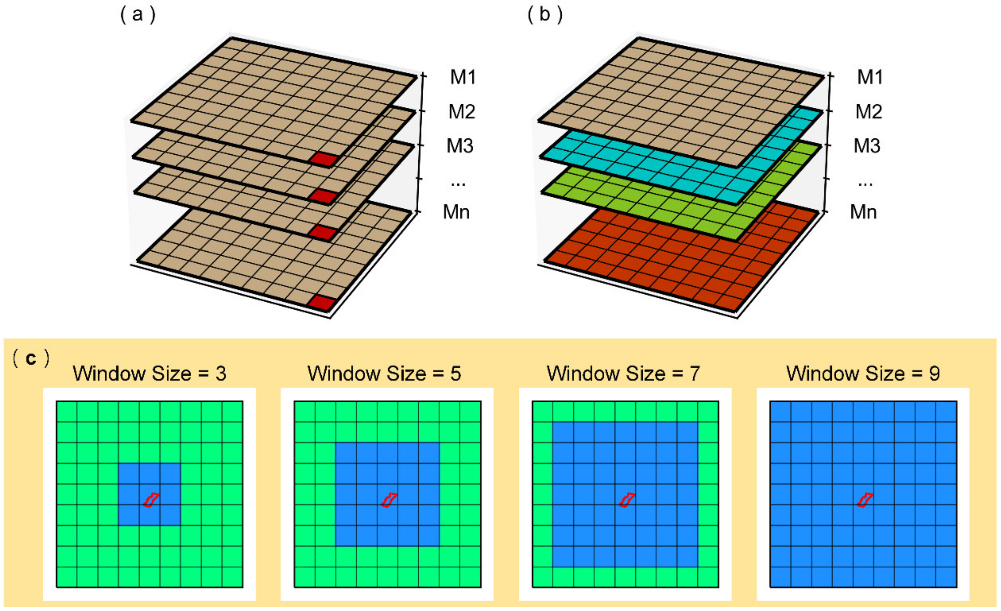
3.1. Study Area

Guantao County and its surrounding region (115°06′–115°40′E, 36°27′–36°47′N) is located in the southern Hebei Province, China, and has an area of approximately 456 km2 [53], as shown in Figure 2. The terrain of the study area slopes from the southwest to the northeast and is generally flat, with an elevation of about 43 m in the south and 36 m in the north (Figure 2). Additionally, Guantao County is in a typical warm-temperate semi-humid continental monsoon climate area that receives plenty of sunshine. The annual average temperature is 14 °C, and the average temperatures of the coldest month (January) and the hottest month (July) are −2.5 °C and 27 °C, respectively [53]. Due to the lack of rational utilization and effective management of water resources, the groundwater in Guantao County is seriously over-exploited. Generally, the depletion of groundwater has induced a series of ecological and geological problems (e.g., land subsidence, ground fissures, soil salinization) that affect the sustainable economic and social development of the region. Thus, it is crucial to analyze water resources storage changes in Guantao County.

3.2. Materials

The research data used in this study include CSR RL06 Mascon, GLDAS, MODIS, TEMP, and in situ observations, as shown in Table 1. Previous studies have revealed that these climate variables are closely related to TWS changes [50,52].

3.2.1. GRACE Solutions

The GRACE satellites were jointly developed by the National Aeronautics and Space Administration (NASA) and Deutsches Zentrum für Luft- und Raumfahrt (DLR). They were successfully launched in March 2002 and ended their mission in October 2017. Currently, GRACE solutions are mainly divided into two categories: Spherical Harmonic Coefficient (SHC) and Mass Concentration solutions (Mascon). The high-degree and high-order coefficients of SHC products are dominated by high-frequency noise and correlated errors in the north–south direction. Therefore, when applying SHC to estimate global TWS changes, data post-processing such as filtering and de-correlated error algorithms are required [54,55]. Since pre-processing methods, such as degree 1 corrections, C20 (degree 2 order 0) replacement, and the glacial isostatic adjustment (GIA) correction, have been applied to Mascon solutions, post-processing is no longer required when using them. For more detailed information, please refer to the literature [56]. Due to the regularization constraints, Mascon solutions have a higher signal-to-noise ratio than SHC products [57,58]. Hence, this study will analyze the regional TWS changes based on the CSR RL06 Mascon (CSR-M06) that was released by the Center for Space Research (CSR). CSR-M06 has a spatiotemporal resolution of 0.25° × 0.25°, and the monthly average values from January 2004 to December 2009 have been deducted.

3.2.2. GLDAS Model

The Global Land Data Assimilation System (GLDAS) was jointly developed by the Goddard Space Flight Center (GSFC) and the National Centers for Environmental Prediction (NCEP) [59]. Using satellite and surface observation data as the primary material, GLDAS outputs global surface state and flux data based on advanced land surface models and data assimilation methods. Currently, GLDAS products include four land surface models: Noah, Mosaic, CLM, and VIC. This study applies the soil moisture from the Noah, which has spatial resolutions of 0.25° × 0.25° and temporal resolutions of one month, including four different soil moisture depths (SM) (i.e., 0~10 cm, 10~40 cm, 40~100 cm, and 100~200 cm). Since the spatial resolution cannot satisfy the requirements, we resampled the resolution of the GLDAS products to 0.05°.

3.2.3. MODIS Data

The Moderate-resolution Imaging Spectroradiometer (MODIS), which is mounted on the Terra and Aqua satellites, is an essential instrument in the US Earth Observation System (EOS), and it is mainly used to detect the global biological and physical processes. Based on the Penman–Monteith equation and Mu’s improved ET algorithm, the MODIS-MOD16 product uses daily meteorological reanalysis data, land cover, albedo, leaf area index, and enhanced vegetation index as input variables to calculate global land surface evaporation [60,61,62]. The datasets include global evapotranspiration (ET), latent heat flux (LE), potential evapotranspiration (PET), and potential latent heat flux (PLE). The spatial resolution of the MODIS-MOD16 product is 500 m, and its temporal resolution is eight days (MOD16A2) and one year (MOD16A3). This study extracted ET components from the MOD16A2 products, and the 8-day results were averaged to obtain monthly temporal resolution products. The day and night land surface temperature (LST_day and LST_night) with a spatial resolution of 0.05° × 0.05° (~ 5.6 × 5.6 km) and the temporal resolution of one month were obtained from the MODIS-MOD11C3 product (version 6) [63].

3.2.4. TEMP Data

The TEMP is China’s monthly average temperature dataset that is released at the National Qinghai-Tibet Plateau Science Data Center (TPDC) and has a spatial resolution of about 1 km and a period from January 1901 to December 2017. According to the global 0.5° climate data released by CRU and the global high-resolution climate products released by WorldClim, this dataset was downscaled in China through the Delta spatial downscaling method. The observation data of 496 independent weather stations were applied to verify the dataset, which performed well [64,65].

3.2.5. In Situ Observations

The measured data from 21 groundwater wells were collected from the Guantao County Groundwater Monitoring and Management Department to verify the high-resolution GWS results after downscaling. These include shallow groundwater wells and deep groundwater wells. In Figure 2, the black dots show the spatial distribution of the groundwater wells. The groundwater level (GWL) changes can be obtained by subtracting the groundwater depth from the elevation of the groundwater well. The groundwater level anomalies (GWLA) can be obtained by subtracting its own average value from the GWL changes, which can be compared with the GRACE-derived GWSA.

3.3. Machine Learning Algorithms

The ensemble learning algorithm, a research hotspot of machine learning, integrates the training results of multiple “weak learners” to form a “strong learner”. This can improve the generalization ability of the model, thereby improving the prediction accuracy [66,67]. The ensemble learning algorithm has higher accuracy, robustness, and flexibility than the single learning algorithm, and it mainly includes the bagging and boosting algorithm.
The idea of bagging is to form sub-training samples by extracting data from the training dataset according to a specified ratio, and the training results of the sub-training samples are averaged as the final prediction result. Random Forest (RF) [68] and Extra Trees Regressor (ETR) [69] are the representative bagging algorithms. RF, which was first proposed by Breiman in 2001, is an ensemble machine learning algorithm that has demonstrated superior performance [68] and is a popular tool for classification and regression. The randomness in the RF is mainly manifested in two aspects: on the one hand, the same amount of samples is randomly selected from the original training data as training samples; on the other hand, partial features are randomly selected to construct decision trees. This randomness creates a low correlation between the different decision trees, which can improve the robustness and accuracy of the model [68]. ETR, which was developed based on the RF, is a relatively novel ensemble machine learning algorithm. Compared to RF, the ETR splits the descriptors at the node entirely randomly, and each tree is trained with the entire dataset instead of sampling.
Unlike the bagging, boosting is an iterative algorithm that trains the same training samples multiple times. The next iteration adjusts the sample weight according to the previous training dataset and outputs the final result after meeting the requirements. The Adaptive Boosting Regressor (ABR) [70] is a representative boosting algorithm. The ABR algorithm first assigns equal weight to each sample, and the next iteration uses the error of the previous weak learner to update the weight of the sample. Thus, the iteration terminates after meeting the accuracy requirements. The Gradient Boosting Regressor (GBR) is also designed based on boosting and is often used for comparisons with the ABR [71]. Different from the iterative conditions of the ABR algorithm, the GBR algorithm rebuilds the model in the gradient descent direction of the loss function of the previous iteration. Generally, the smaller the loss function, the better the model performance. We can improve the model performance of by decreasing the loss function along the gradient direction. The ensemble learning algorithm is widely used in the field of earth science because of its strong ability to deal with nonlinear problems. In the research focusing on the downscaling of GRACE data, RF and GBR have more applications, but there are few discussions about ETR and ABR. Therefore, this study utilizes RF, ETR, ABR, and GBR to downscale GRACE data and selects the best performing algorithm for analysis in the next section. These four machine learning algorithms can be called in Python’s scikit-learn function library [72].

3.4. Data Processing Flow

The data processing in the research aims to set up modeling windows, optimize the combined model, obtain high-resolution TWSA and GWSA, and use in situ groundwater well observations to verify the downscaled results. The downscaling process is shown in Figure 3. The red arrow represents the input data, the blue arrow represents the output downscaling models and results, and the green arrow represents the validation data:
(1)
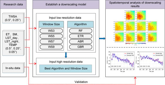
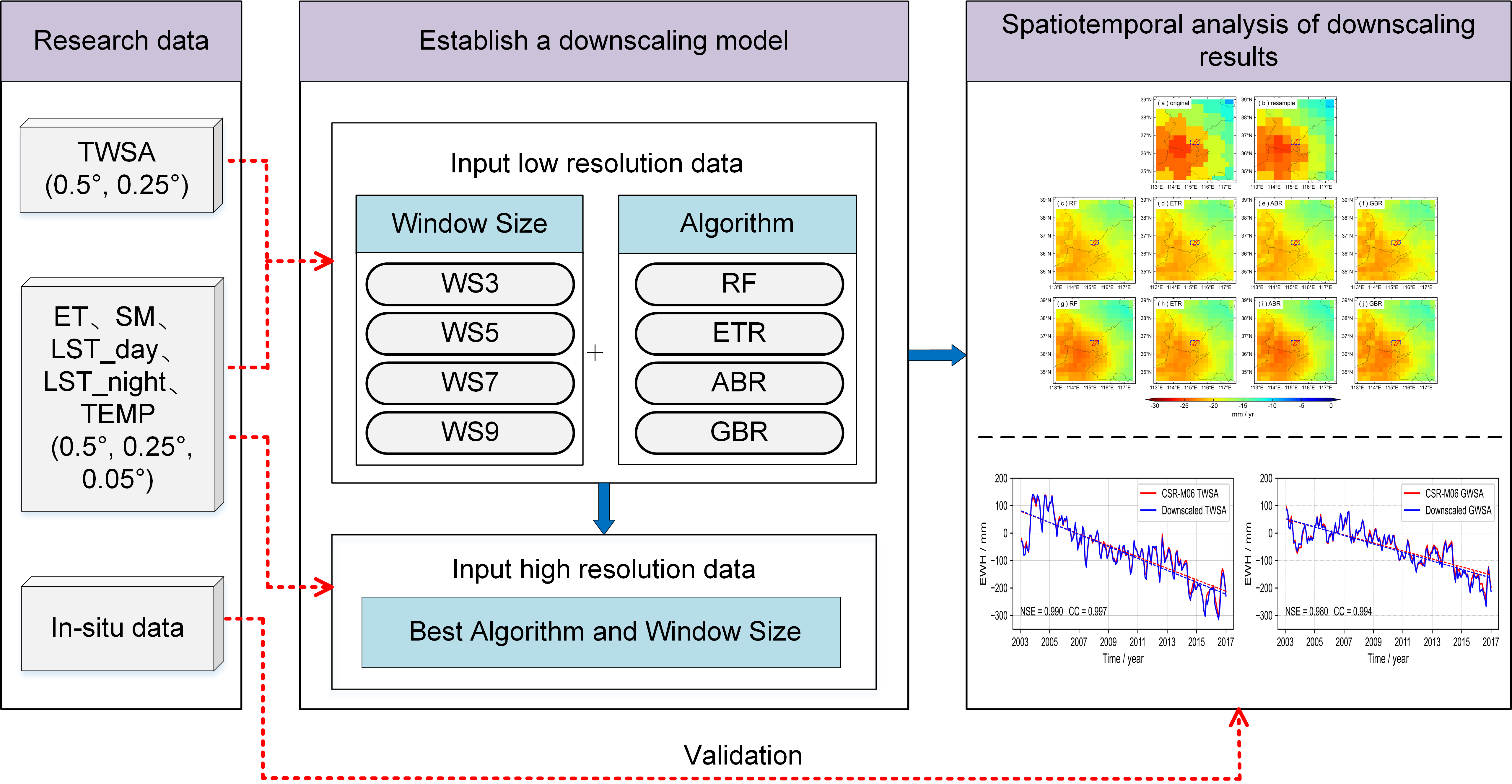
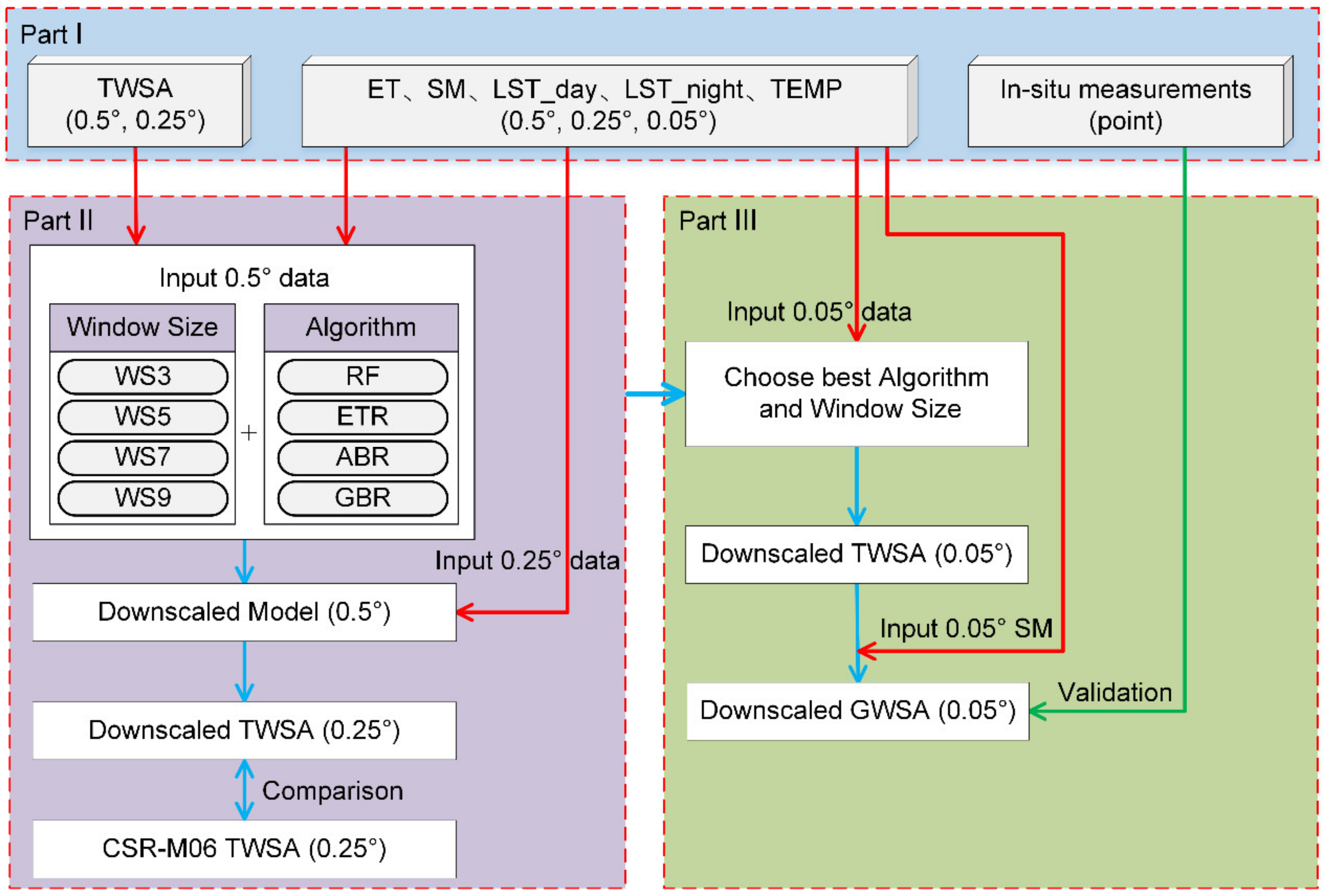
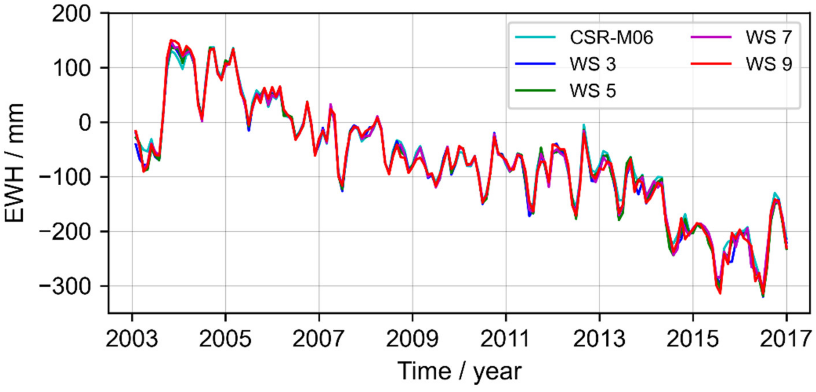
Firstly, to analyze the influence of the modeling window on the downscaled results, we set up modeling windows with the sizes of 3 × 3 (WS3), 5 × 5 (WS5), 7 × 7 (WS7), and 9 × 9 (WS9) based on a 0.5° grid with Guantao County as the center (Figure 1c).
(2)
Secondly, due to the inconsistent spatiotemporal resolution, the research data needed to be preprocessed (Part I). The spatial resolution of TWSA was resampled to 0.5° and 0.25°; the spatial resolution of ET, SM, LST_day, LST_night, and TEMP was resampled to 0.5°, 0.25°, and 0.05°. With the exception of the in situ groundwater well observations, the temporal resolution of other research data is unified as one month.
(3)
Thirdly, The MLSDM is employed to establish the regression models between TWSA and five hydrological variables at a spatiotemporal resolution of 0.5° × 0.5° and one month (Figure 1b,c and Part II) (WS3, WS5, WS7, WS9 modeling window cross joint RF, ETR, GBR, ABR algorithm, such as WS3 + RF). We input the hydrological variables of 0.25° into the regression model of the corresponding month (the red arrow in Part II) to obtain the downscaled 0.25° TWSA. Then, this study compared RMSE, MAE, NSE, and CC between downscaled 0.25° TWSA and CSR-M06-derived TWSA on spatiotemporal signals to determine the best combined model.
(4)
Finally, the optimal combined model in Part II was applied to the hydrological variables at a spatial resolution of 0.05° to obtain the estimated 0.05° TWSA. According to the water storage balance equation, the soil moisture anomalies (SMA) were subtracted from the TWSA to estimate a 0.05° GWSA. Subsequently, the in situ groundwater well observations in Guantao County were used to compare and verify the downscaled GWSA (Part III).

3.5. Model Evaluation Metrics

In this study, four metrics were utilized to evaluate the downscaled results of the above design schemes, namely RMSE, MAE, NSE, and CC. The calculation equations are as follows [73,74,75,76,77]:
R M S E = 1 n i = 1 n Y i X i 2
M A E = 1 n i = 1 n Y i X i
N S E = 1 i = 1 n Y i X i 2 i = 1 n X i X ¯ 2
C C = i = 1 n X i X ¯ Y i Y ¯ i = 1 n X i X ¯ 2 i = 1 n Y i Y ¯ 2
where Y is the observed value, X is the predicted value, Y ¯ and X ¯ are the mean values of Y and X, respectively, and n is the number of datasets. For the model construction, the higher the correlation coefficient NSE and CC between the observed value and predicted value, the better the model accuracy. The smaller the RMSE and MAE, the closer the predicted value was to the observed value and the higher the accuracy of the model.

4. Results

4.1. Accuracy Analysis of Downscaling Method

4.1.1. Performance of Downscaling Model

According to Section 3.4, the monthly regression relationship between TWSA and five hydrological variables was established using the WS3, WS5, WS7, and WS9 modeling windows cross-combined with the RF, ETR, ABR, and GBR. In this way, the TWSA data was downscaled from 0.5° to 0.25°. Figure 4 shows the average RMSE, MAE, NSE, and CC of the validation set of the combined downscaling model. Overall, the results of each combined downscaling model have satisfactory performance. The RMSE and MAE are between 6.77~13.62 mm and 3.36~10.21 mm, respectively. Meanwhile, the NSE and CC are not less than 0.51 and 0.76. In WS3, WS5, WS7, and WS9, the RMSE of the ETR were 6.77 mm, 9.94 mm, 9.56 mm, and 10.90 mm, respectively (the MAE of the ETR are 3.36 mm, 4.62 mm, 4.32 mm, and 4.85 mm, respectively), which are better than other algorithms, and the NSE and CC of the ETR have the maximum value in each modeling window. The comparison indicates that the ETR is slightly superior to RF, ABR, and GBR in terms of the model accuracy statistics.

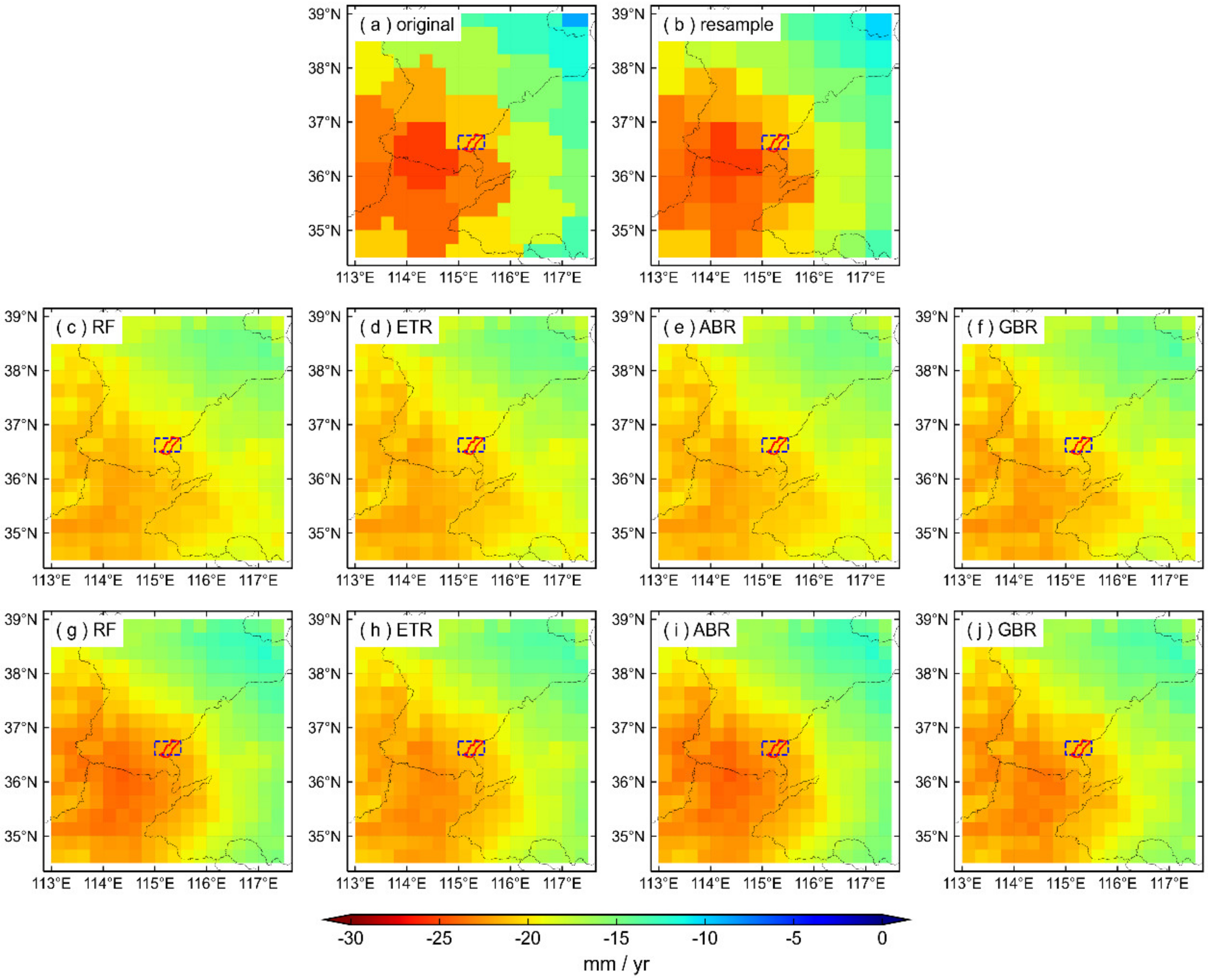
4.1.2. Spatial Analysis of Downscaled TWSA before and after Adding Residuals

After training the low-resolution hydrological variables with the combined downscaling models, there is a residual error between the output predicted value and the original value. Previous studies have shown that it can improve the downscaling accuracy by interpolating the residuals to a higher resolution through the Kriging method and then adding them to the downscaled results with a high resolution [42,78,79]. Therefore, although the ETR algorithm has slightly better performance, it is necessary to further evaluate the accuracy of each combined downscaling model. In order to display the distribution of the TWSA signals in the entire study area, Figure 5 shows the spatial distribution of the TWSA trends from 0.5° downscaling to 0.25° in WS9. Figure 5a shows the TWSA trend with a spatial resolution of 0.25° derived by CSR-M06 from January 2003 to December 2016; Figure 5b shows the TWSA trend from 0.25° resampling to 0.5°; Figure 5c–j are the results of different combined downscaling models. On the whole, the spatial distribution of the downscaled signal and the original signal have great consistency, both of which show that the TWSA declines severely in the southwest and slightly declines in the northeast (Figure 5c–f). After adding the residuals, the consistency of the spatial distribution of the downscaled TWSA and original TWSA is improved (Figure 5g–j). The downscaled signals of the WS3, WS5, and WS7 modeling windows all demonstrated similar performance.
To further analyze the accuracy, we calculated the spatial distribution consistency of the CSR-M06 TWSA and downscaled TWSA, including the signal before and after adding residuals (Figure 6). After adding residuals, the accuracy of each combined downscaling model is improved. The RMSE values decreased from 1.69~2.55 mm/yr to 1.36~1.89 mm/yr; The MAE values decreased from 1.19~2.10 mm/yr to 1.03~1.53 mm/yr; The NSE values increased from 0.28~0.69 to 0.51~0.87; The CC values increased from 0.73~0.88 to 0.75~0.94 (Figure 6). The RMSE, MAE, NSE, and CC increased by 20~26%, 13~27%, 20~82%, and 3~7%, respectively. The downscaling accuracy of the RF in each modeling window is better than other that of the algorithms after adding the residuals. Taking WS5 as an example, the RMSE and MAE of RF are the smallest, at 1.36 mm/yr and 1.12 mm/yr, respectively, and NSE and CC are both the largest, at 0.82 and 0.93, respectively. These results indicate that after the GRACE grid data are downscaled by the RF, the downscaled signal is closer to the original signal in spatial distribution.

4.1.3. Time Series Analysis of TWSA in Guantao County before and after Downscaling

From the spatial signal analysis in Section 4.1.2, it is known that the downscaling accuracy of the RF is better. Subsequently, this section analyzes the downscaling accuracy of the WS3, WS5, WS7, and WS9 modeling windows combined with RF from the temporal dimension. Figure 7 shows the TWSA time series in Guantao County (the small rectangle in Figure 5: 115.0°–115.5°E, 36.5°–36.75°N), including the CSR-M06 and the downscaled results of different modeling windows combined with RF. With the exception of several time nodes (e.g., the beginning of 2004, the beginning of 2014, the end of 2015), the TWSA time series in Guantao County derived by the downscaled results and the CSR-M06 model are in good agreement (Figure 7). To analyze the accuracy of each combination model in Figure 7, regression analysis was performed on the downscaled results and the CSR-M06 model (Figure 8). The NSE and CC of the downscaled results of the four modeling windows combined with the RF are both greater than 0.98. This demonstrates that the downscaled results of each modeling window combined with RF have high accuracy (Figure 8). The RMSE, MAE, NSE, and CC values of WS5 are 9.67 mm, 6.80 mm, 0.990, and 0.997, respectively, which are better than WS3, WS7, and WS9. The statistical accuracy of the WS3 and WS7 modeling windows is the second best, and the statistical accuracy of the WS9 modeling window is the worst.

4.2. Downscaled Results with High Spatial Resolution

4.2.1. Spatiotemporal Distribution of TWSA Downscaled Signal

To further satisfy the analysis of the TWS changes in Guantao County, this section utilizes WS5 combined with RF to obtain TWSA with a spatial resolution of 0.05°. Figure 9 shows the spatial distribution of the TWSA trends before and after downscaling from January 2003 to December 2016. In the WS5 modeling window, the spatial distribution of the signals is highly consistent before and after downscaling, which shows that the TWS decreases rapidly in the southwest and central regions and decreases slowly in the northeast. Moreover, the downscaled signal can better reflect the detailed characteristics of the TWS changes. Meanwhile, the CSR-M06 TWSA and 0.05°downscaling results are used to calculate the TWSA time series in Guantao County (Figure 10). The NSE and CC of the two time series are above 0.99 and decrease at −20.86 mm/yr and −21.79 mm/yr, respectively.

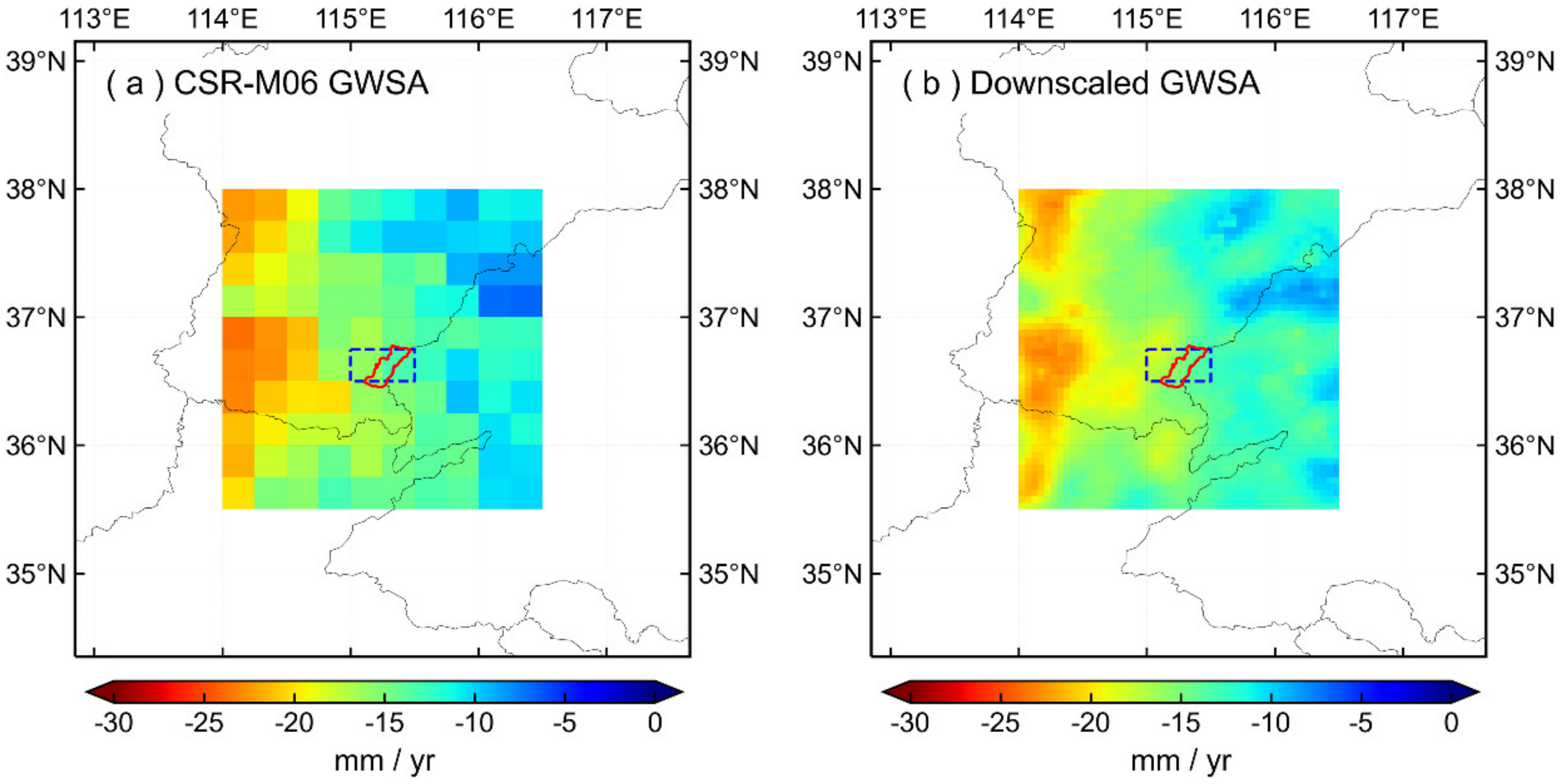
4.2.2. Spatiotemporal Distribution of GWSA Downscaled Signal

According to the water storage balance equation, the SM are subtracted from the TWS to estimate the regional GWS. Figure 11 shows the spatial distribution of the GWSA after removing the SMA from the same spatial resolution from the CSR-M06 TWSA and 0.05° downscaled TWSA. The spatial distribution of GWSA before and after downscaling is in good agreement, with a severe decrease in the western region and a slight decrease in the eastern region (Figure 11). Similarly, the GWSA time series in Guantao County are calculated (Figure 12). The NSE and CC of the downscaled GWSA and the CSR-M06-derived GWSA are 0.980 and 0.994, respectively. The GWSA trends in Guantao County calculated by CSR-M06 model and the 0.05° downscaled results are −14.53 mm/yr and −15.46 mm/yr, respectively (Figure 12). The discussion shows that the downscaling method proposed in this study can not only improve the spatial resolution of GRACE data but also effectively preserves the original signal.

5. Discussion

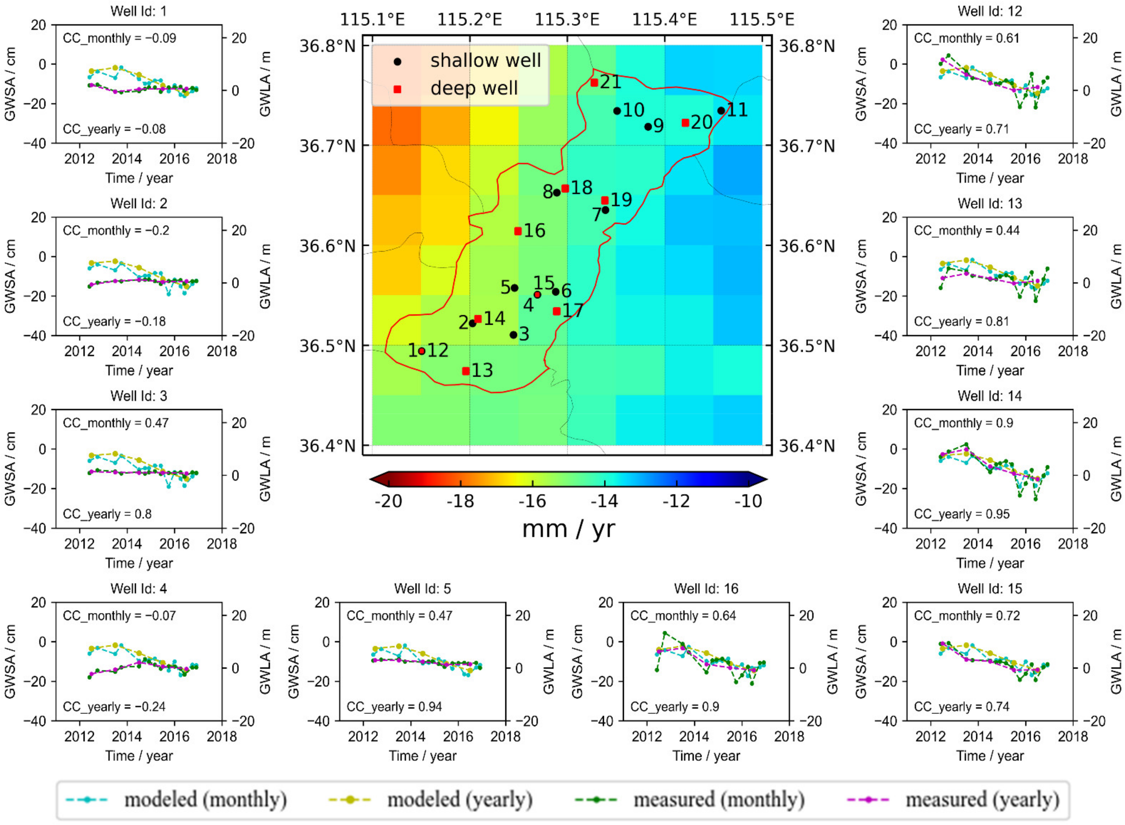
5.1. Validation Analysis of In Situ Observations

To analyze the reliability of high-resolution GWSA (0.05°) after downscaling, this study collects observational data from 21 groundwater wells in Guantao County for verification. There are 11 shallow groundwater wells (No. 1~11) and 10 deep groundwater wells (No. 12~21). The public period for GWSA and measured groundwater data is from 2012~2016. Due to the significant uncertainty of the specific yield, this study mainly analyzes the GWSA and measured groundwater change trends and their correlations. Figure 13 shows the spatial distribution of groundwater logging and part of the GWS time series. The black dots and red dots represent shallow and deep groundwater wells, respectively. We calculated the correlation coefficients (CC_monthly and CC_yearly) of the measured and inverted groundwater on the monthly and yearly time scales, as shown in Figure 13 and Table 2. Most of the measured data and the GWSA show a downward trend (Figure 13). Table 2 shows the CC between the GWLA and the GWSA. The observation data from the shallow groundwater wells have poor consistency with the downscaled GWSA. The CC of observation wells 3, 5, and 6 are positive, and the others are negative. With the exception of the poor correlation between observation wells 18 and 19, the CC_monthly and CC_yearly of other deep groundwater wells are above 0.43 and 0.70, respectively. By comparing the observation wells at different depths with the GWSA, it is shown that the overexploitation of deep groundwater may mainly cause groundwater loss in Guantao County. Furthermore, compared to the CC before downscaling, most of the CC after downscaling are improved, indicating that the downscaling work is effective (Table 2).

5.2. Limitation and Outlook

From the above discussion, we know that the MLSDM proposed in this study can achieve good results when TWSA is downscaled. The downscaling model established in WS5 (~250 km × 250 km) has the best accuracy, indicating that the modeling window size needs to be analyzed when the downscaling model is established in the spatial dimension. Therefore, it is necessary to consider the influence of surrounding hydrological conditions on the study region during the downscaling process. Meanwhile, compared to downscaling in the temporal dimension, downscaling in the spatial dimension effectively alleviates the spatial discontinuity of the downscaled results between grids. In this study, the downscaled results of GWSA are compared with the in situ groundwater well observations. However, the in situ groundwater well observations are limited, and there is only 5 years of overlap with GRACE products. The long-term changes of the downscaled GWSA result cannot be effectively verified. In later work, we hope to obtain more measured data spanning a longer time period and a regular observation time to compare and analyze the seasonal changes of the downscaled GRACE products. In addition, follow-up work can consider integrating the downscaling results and the measured data that have good accuracy through data assimilation. This process can correct the downscaling results to further improve the downscaling accuracy. Generally, the method of establishing the TWSA downscaling model in the spatial dimension can achieve good results in Guantao County. Nevertheless, we still need more experimental analysis in other regions.

6. Conclusions

Fully understanding the changes in regional water resources is essential for its rational utilization and effective management. GRACE products have been widely used to analyze the TWS and GWS changes in large areas, but it is still a challenge to analyze the water storage changes in small areas. To satisfy small-scale regional water resources monitoring needs in smaller areas, this research proposes a new machine learning spatial downscaling method (MLSDM) that can effectively improve the spatial resolution of TWSA/GWSA. Compared to building downscaling models on a single grid, the MLSDM can improve the spatial discontinuity of the downscaled signals. This study discusses the accuracy of the downscaled results obtained by combining RF, ETR, ABR, and GBR for WS3, WS5, WS7, and WS9. The results are as follows:
(1)
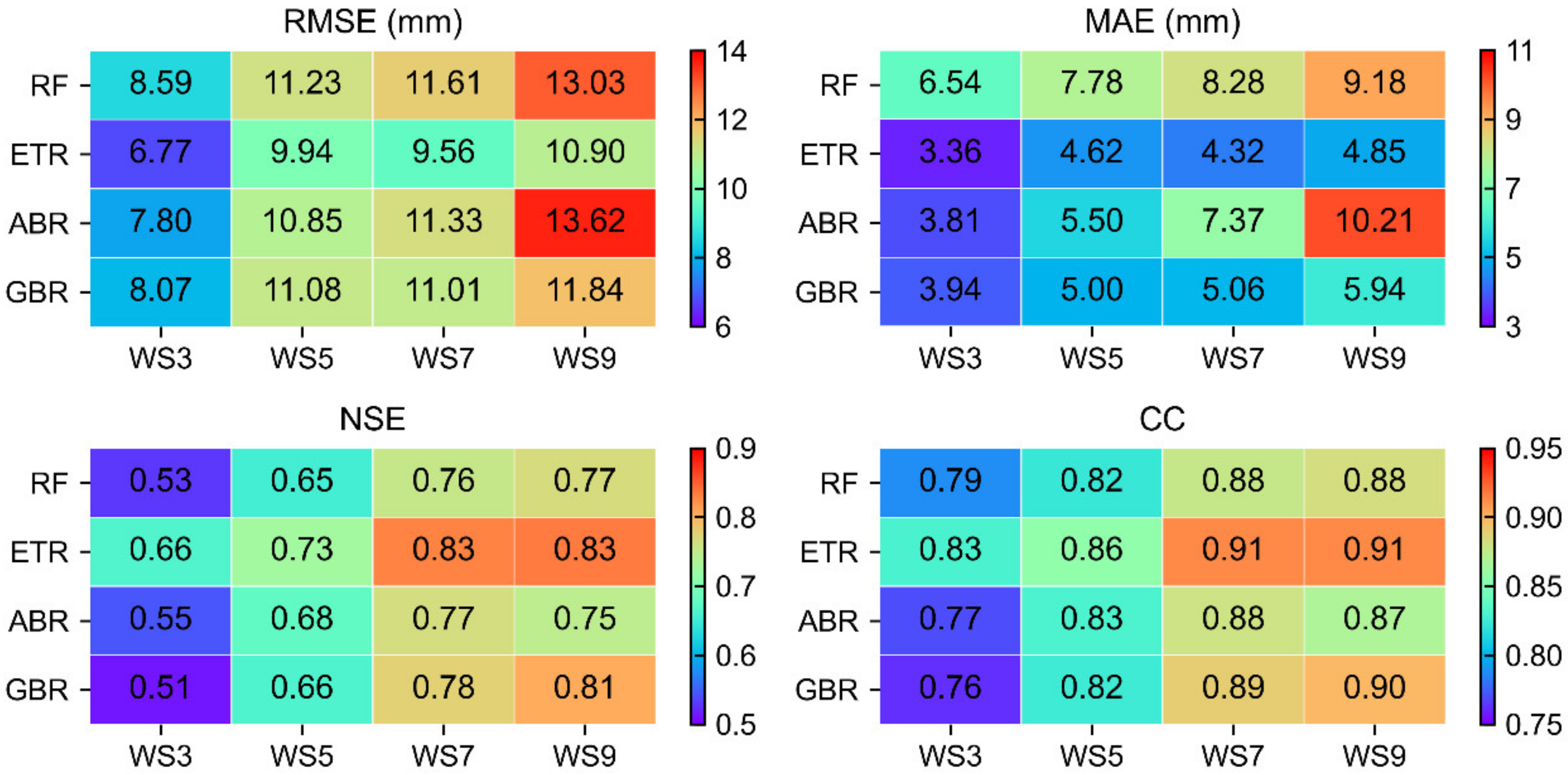
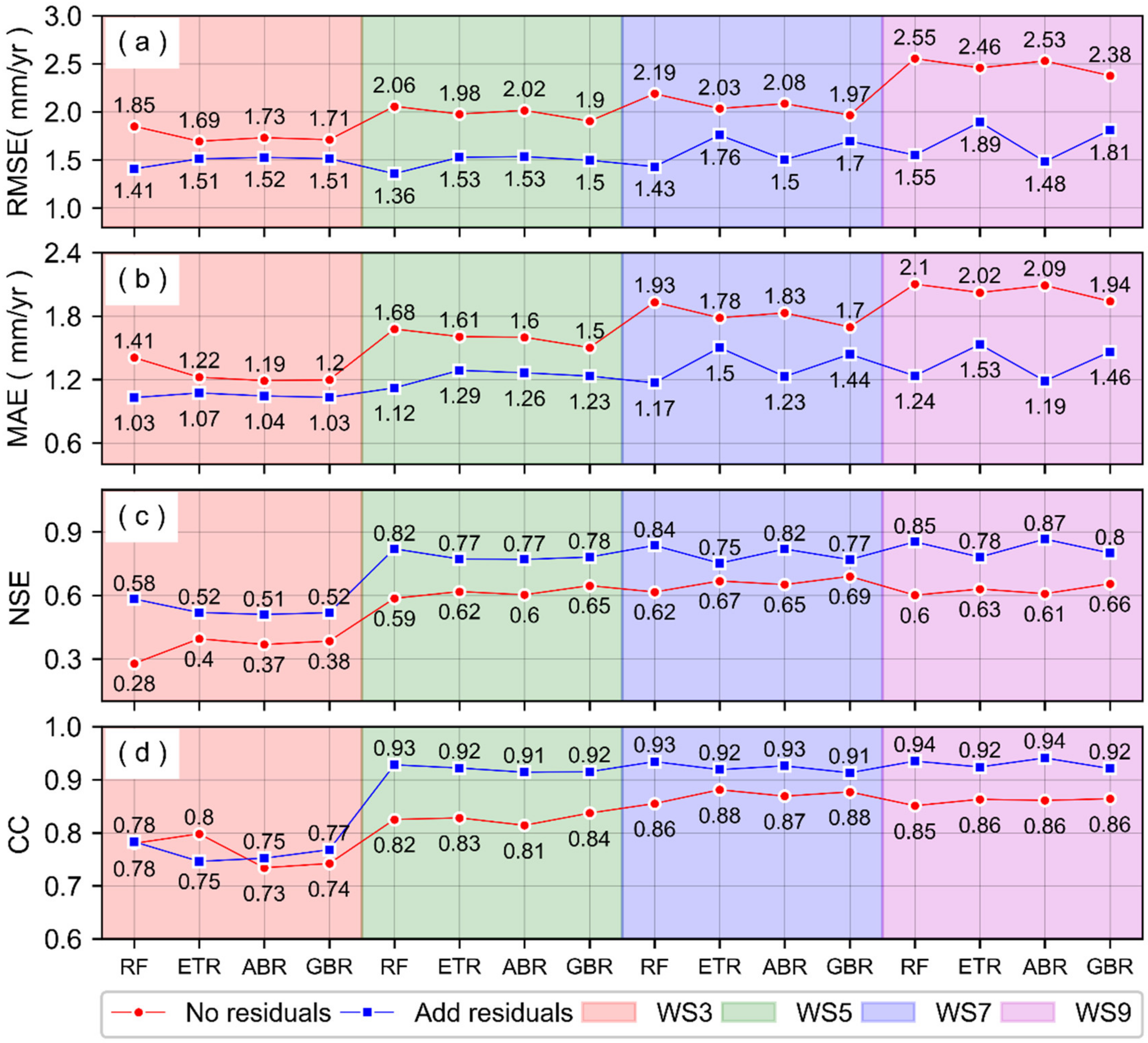
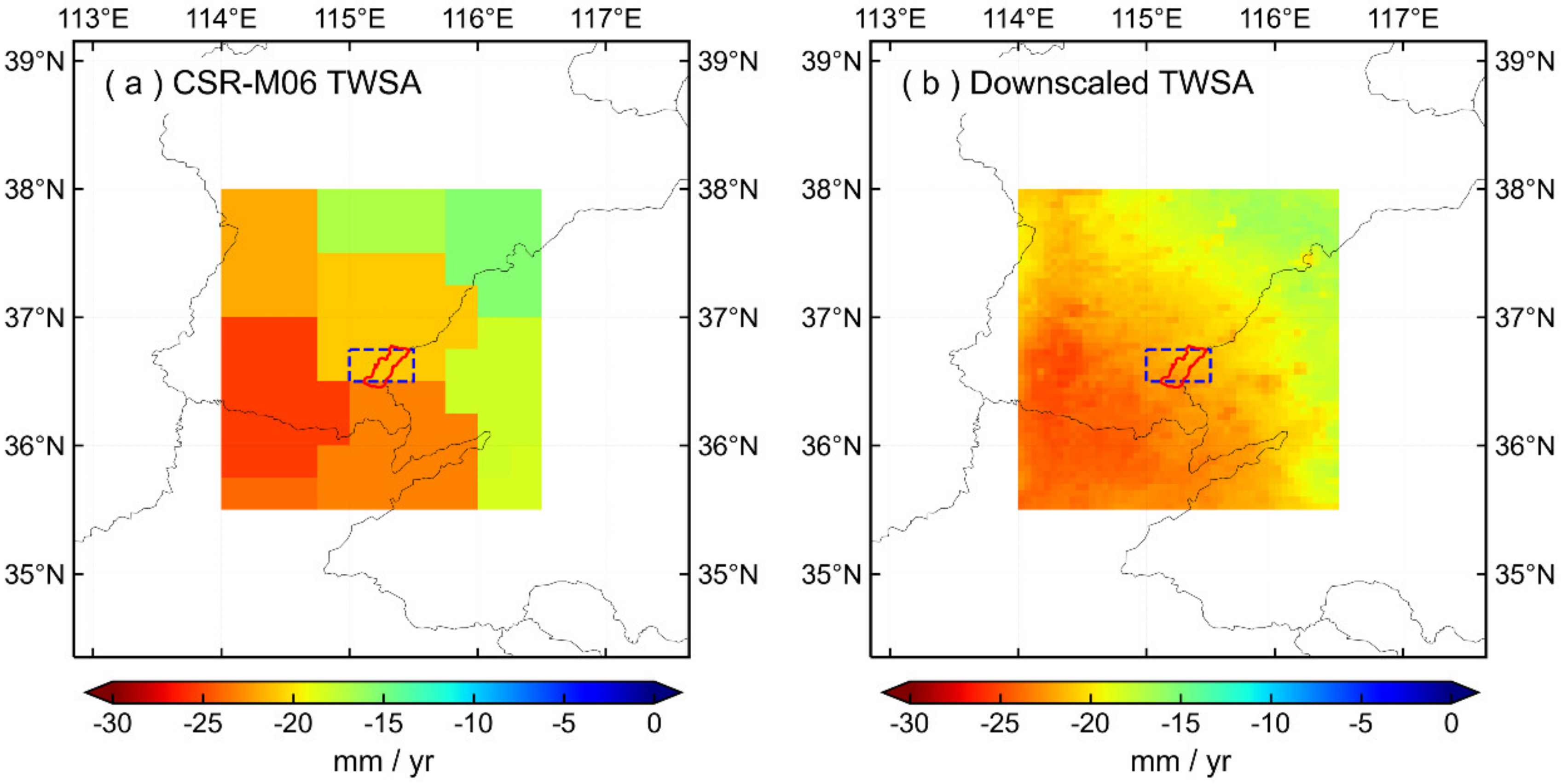
To improve the spatial resolution of TWSA products, the MLSDM was constructed using different modeling windows combined with multiple machine learning algorithms. The verification results show that the downscaled results obtained by MLSDM are consistent with the original CSR-M06 model in the spatial distribution. Furthermore, after adding residuals, the downscaling accuracy of each combined model was improved, and the RMSE, MAE, NSE, and CC values increased by 20%~26%, 13%~27%, and 20%~82%, and 3%~7%. Specifically, the accuracy of RF in each modeling window is slightly better than ETR, ABR, and GBR.
(2)
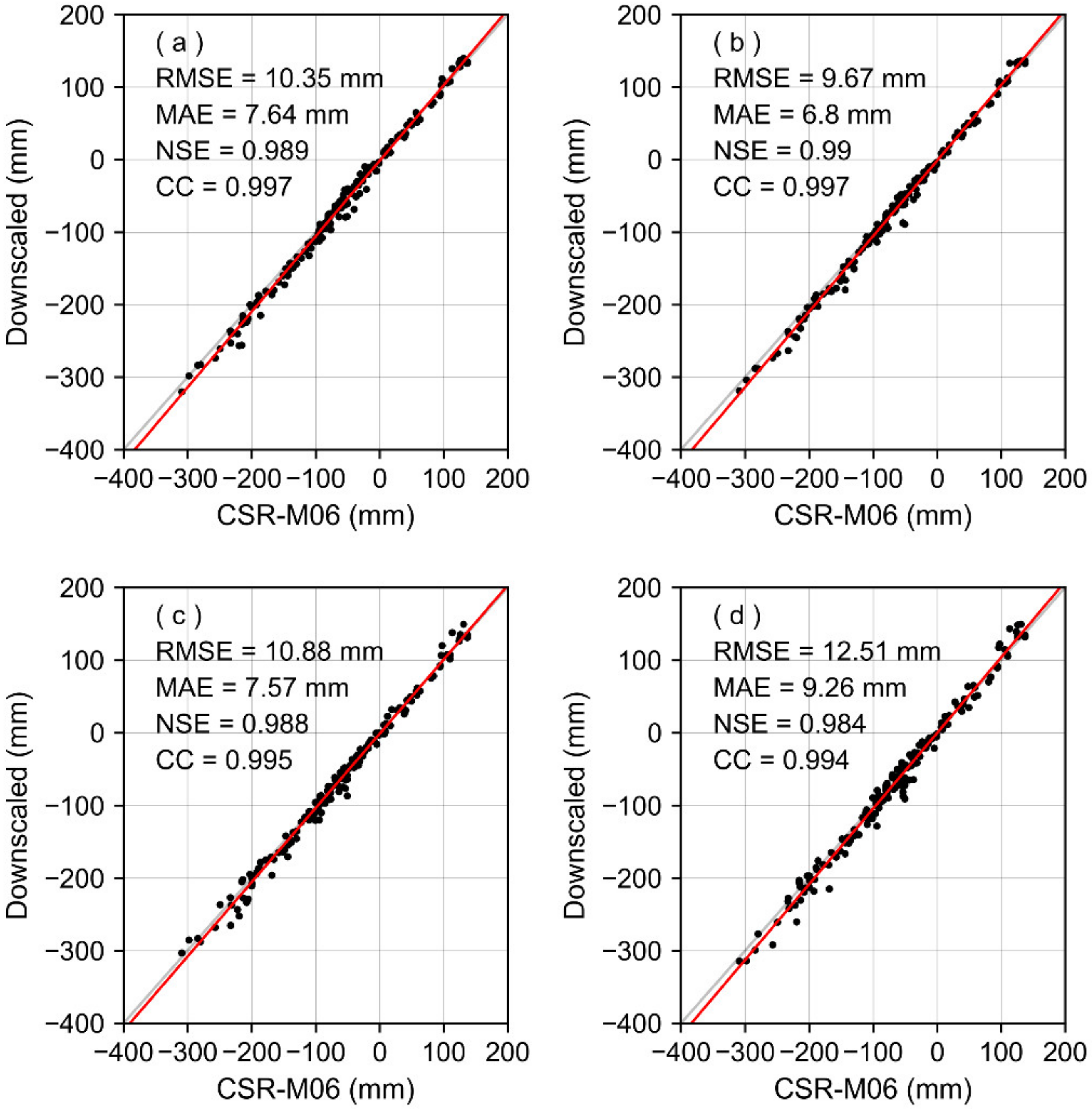
To further analyze the impact of the modeling windows, this study compared the TWS time series changes in Guantao County that were derived from the downscaled results of RF combined with different modeling windows. The RMSE, MAE, NSE, and CC of WS5 combined with RF were 9.67 mm, 6.80 mm, 0.990, and 0.997, respectively, which are slightly superior to the downscaled results of WS3, WS7, and WS9.
(3)
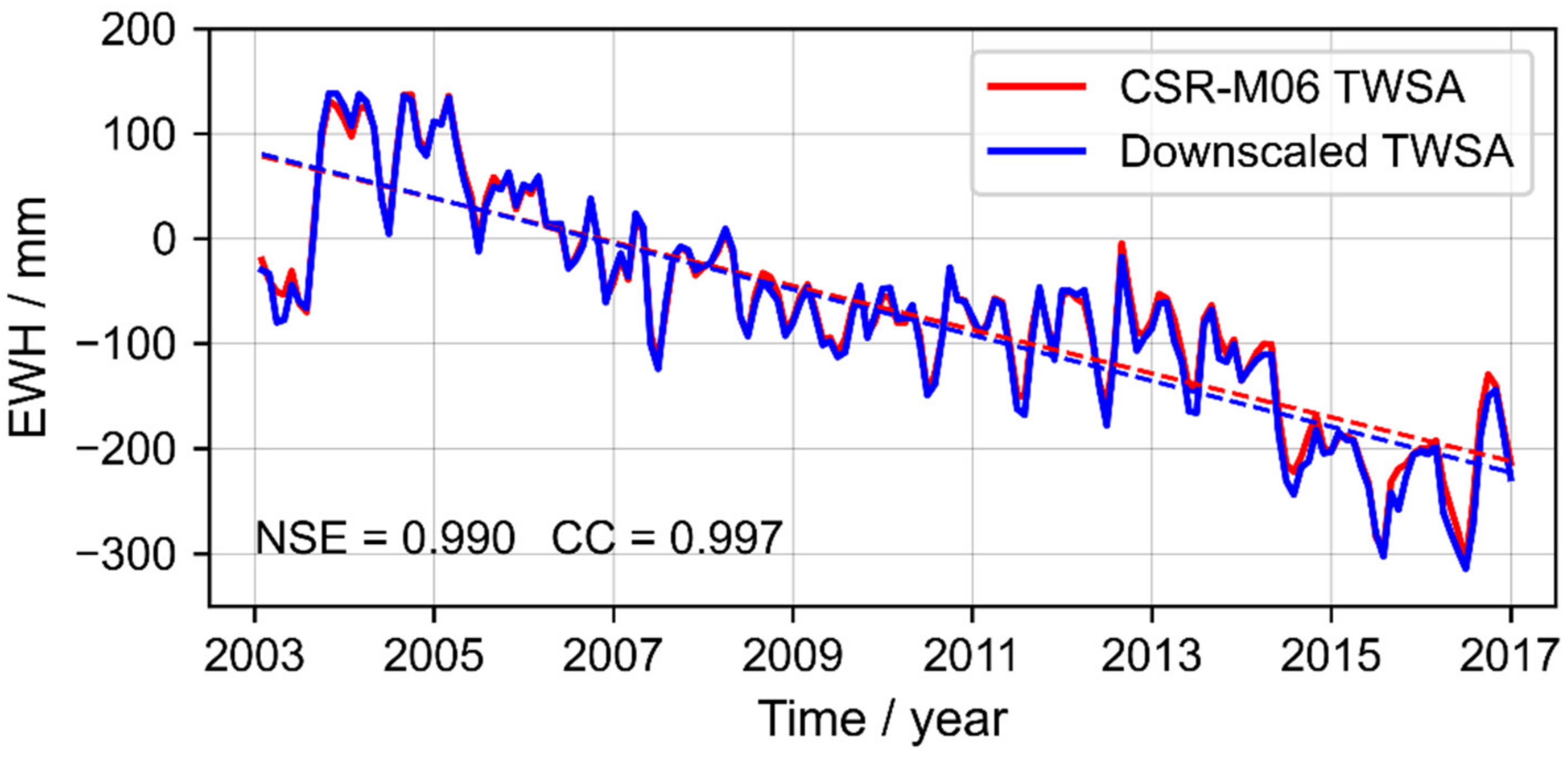
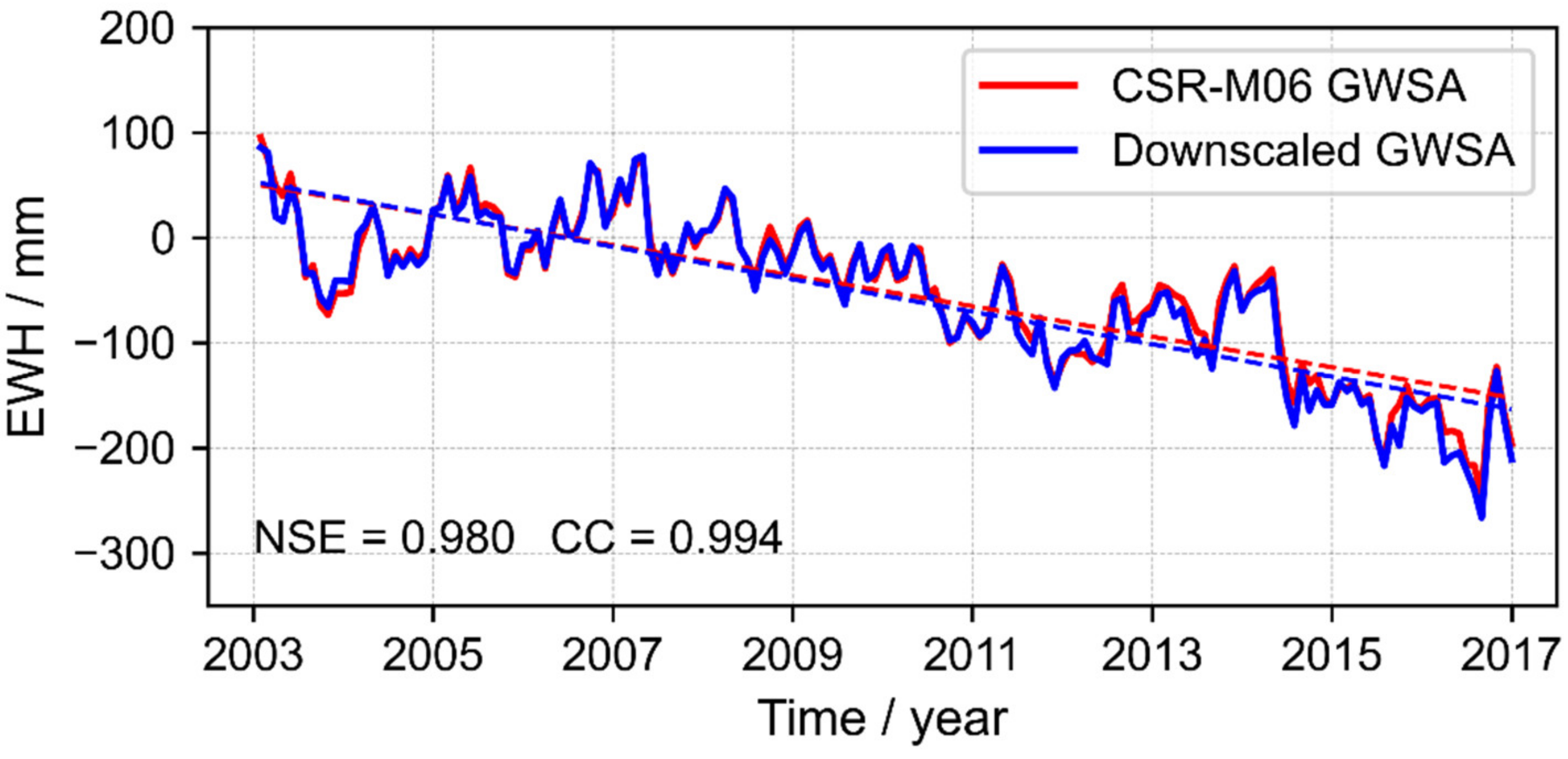
The combined model of WS5 and RF was utilized to downscale the TWSA/GWSA data to 0.05°, and the signals before and after downscaling demonstrated high consistency. The NSE and CC of the TWSA time series before and after downscaling are 0.990 and 0.997, respectively, and the NSE and CC of GWSA time series before and after downscaling are 0.980 and 0.994, respectively. Subsequently, the measured groundwater level data was used to verify the high-resolution GWSA results. The CC between the high-resolution GWSA and 80% of the deep groundwater well data was above 0.70, but the correlation between shallow groundwater was relatively poor.
Through the above results, we conclude that the downscaled work based on the MLSDM not only improved the spatial resolution of TWSA/GWSA, but also maintained the spatial distribution of the original TWSA/GWSA signal. Data with a high spatial resolution can provide relevant guidance for in-depth investigations of regional water resources and can help improve future hydrological research in small-scale areas, thereby enhancing the sustainable water resource management. Nevertheless, we realize that the downscaling of TWSA/GWSA is still a challenge, and more discussions on this issue are needed in the future.

Author Contributions

All authors collaborated to conduct this study; Z.C.: scientific analysis, manuscript writing, and editing; W.Z. and W.Y.: experiment design, project management; W.Z., W.Y. and X.L.: review and editing; G.Z. and J.Z.: data curation; Z.C. and G.Z.: processing of GRACE data. All authors contributed to the article and approved the submitted version. Z.C., W.Z. and W.Y. contributed equally to this paper. All authors have read and agreed to the published version of the manuscript.

Funding

This work was supported by the National Natural Science Foundation of China under Grant (41774014, 41574014), the Liaoning Revitalization Talents Program under Grant (XLYC2002082), the Frontier Science and Technology Innovation Project and the Innovation Workstation Project of Science and Technology Commission of the Central Military Commission under Grant (085015), and the Outstanding Youth Fund of China Academy of Space Technology.

Institutional Review Board Statement

Not applicable.

Informed Consent Statement

Not applicable.

Data Availability Statement

No new data were created or analyzed in this study. Data sharing is not applicable to this article.

Acknowledgments

The authors greatly appreciate the National Aeronautics and Space Administration (NASA) for the GRACE CSR RL06 Mascon data; we also thank the Goddard Earth Sciences Data and Information Center (GES DISC) for providing the Global Land Data Assimilation System (GLDAS) data and the US Earth Observation System (EOS) for providing the MODIS data.

Conflicts of Interest

The authors declare no conflict of interest.

References

  1. Döll, P.; Hoffmann-Dobrev, H.; Portmann, F.T.; Siebert, S.; Eicker, A.; Rodell, M.; Strassberg, G.; Scanlon, B.R. Impact of water withdrawals from groundwater and surface water on continental water storage variations. J. Geodyn. 2012, 59–60, 143–156. [Google Scholar] [CrossRef]
  2. Wada, Y.; Wisser, D.; Bierkens, M.F.P. Global modeling of withdrawal, allocation and consumptive use of surface water and groundwater resources. Earth Syst. Dyn. 2014, 5, 15–40. [Google Scholar] [CrossRef] [Green Version]
  3. Dangar, S.; Asoka, A.; Mishra, V. Causes and implications of groundwater depletion in India: A review. J. Hydrol. 2021, 596, 126103. [Google Scholar] [CrossRef]
  4. Feng, W.; Zhong, M.; Lemoine, J.-M.; Biancale, R.; Hsu, H.-T.; Xia, J. Evaluation of groundwater depletion in North China using the Gravity Recovery and Climate Experiment (GRACE) data and ground-based measurements. Water Resour. Res. 2013, 49, 2110–2118. [Google Scholar] [CrossRef]
  5. Scanlon, B.R.; Longuevergne, L.; Long, D. Ground referencing GRACE satellite estimates of groundwater storage changes in the California Central Valley, USA. Water Resour. Res. 2012, 48, W04520.04521–W04520.04529. [Google Scholar] [CrossRef] [Green Version]
  6. Khan, A.A.; Zhao, Y.; Khan, J.; Rahman, G.; Rafiq, M.; Moazzam, M.F.U. Spatial and Temporal Analysis of Rainfall and Drought Condition in Southwest Xinjiang in Northwest China, Using Various Climate Indices. Earth Syst. Environ. 2021, 5, 201–216. [Google Scholar] [CrossRef]
  7. Valipour, M.; Bateni, S.M.; Jun, C. Global Surface Temperature: A New Insight. Climate 2021, 9, 81. [Google Scholar] [CrossRef]
  8. Bierkens, M.F.P.; Wada, Y. Non-renewable groundwater use and groundwater depletion: A review. Environ. Res. Lett. 2019, 14, 063002. [Google Scholar] [CrossRef]
  9. Tapley, B.D.; Bettadpur, S.; Ries, J.C.; Thompson, P.F.; Watkins, M.M. GRACE Measurements of Mass Variability in the Earth System. Science 2004, 305, 503–505. [Google Scholar] [CrossRef] [Green Version]
  10. Wahr, J.; Swenson, S.; Zlotnicki, V.; Velicogna, I. Time-variable gravity from GRACE: First results. Geophys. Res. Lett. 2004, 31, L11501. [Google Scholar] [CrossRef] [Green Version]
  11. Famiglietti, J.S.; Rodell, M. Water in the Balance. Science 2013, 340, 1300–1301. [Google Scholar] [CrossRef]
  12. Alley, W.M.; Konikow, L.F. Bringing GRACE Down to Earth. Groundwater 2015, 53, 826–829. [Google Scholar] [CrossRef]
  13. Hasan, E.; Tarhule, A.; Kirstetter, P.-E. Twentieth and Twenty-First Century Water Storage Changes in the Nile River Basin from GRACE/GRACE-FO and Modeling. Remote Sens. 2021, 13, 953. [Google Scholar] [CrossRef]
  14. Scanlon, B.; Zhang, Z.; Rateb, A.; Sun, A.; Wiese, D.; Save, H.; Beaudoing, H.; Lo, M.-H.; Müller Schmied, H.; Doell, P.; et al. Tracking Seasonal Fluctuations in Land Water Storage Using Global Models and GRACE Satellites. Geophys. Res. Lett. 2019, 46, 5254–5264. [Google Scholar] [CrossRef]
  15. Yan, X.; Zhang, B.; Yao, Y.; Yang, Y.; Li, J.; Ran, Q. GRACE and land surface models reveal severe drought in eastern China in 2019. J. Hydrol. 2021, 601, 126640. [Google Scholar] [CrossRef]
  16. Xiong, J.; Guo, S.; Yin, J.; Gu, L.; Xiong, F. Using the Global Hydrodynamic Model and GRACE Follow-On Data to Access the 2020 Catastrophic Flood in Yangtze River Basin. Remote Sens. 2021, 13, 3023. [Google Scholar] [CrossRef]
  17. Chen, J.L.; Wilson, C.R.; Tapley, B.D. Contribution of ice sheet and mountain glacier melt to recent sea level rise. Nat. Geosci. 2013, 6, 549. [Google Scholar] [CrossRef]
  18. Cazenave, A.; Chen, J. Time-variable gravity from space and present-day mass redistribution in theEarth system. Earth Planet. Sci. Lett. 2010, 298, 263–274. [Google Scholar] [CrossRef]
  19. Rodell, M.; Chen, J.; Kato, H.; Famiglietti, J.S.; Nigro, J.; Wilson, C.R. Estimating groundwater storage changes in the Mississippi River basin (USA) using GRACE. Hydrogeol. J. 2007, 15, 159–166. [Google Scholar] [CrossRef] [Green Version]
  20. Chen, J.; Famigliett, J.S.; Scanlon, B.R.; Rodell, M. Groundwater Storage Changes: Present Status from GRACE Observations. Remote Sens. Water Resour. 2016, 207–227. [Google Scholar] [CrossRef] [Green Version]
  21. Chen, J.L.; Wilson, C.R.; Tapley, B.D.; Yang, Z.L.; Niu, G.Y. 2005 drought event in the Amazon River basin as measured by GRACE and estimated by climate models. J. Geophys. Res. Solid Earth 2009, 114, B05404. [Google Scholar] [CrossRef]
  22. Chen, J.L.; Wilson, C.R.; Tapley, B.D. The 2009 exceptional Amazon flood and interannual terrestrial water storage change observed by GRACE. Water Resour. Res. 2010, 46, W12526. [Google Scholar] [CrossRef] [Green Version]
  23. Zhou, H.; Luo, Z.; Tangdamrongsub, N.; Wang, L.; He, L.; Xu, C.; Li, Q. Characterizing Drought and Flood Events over the Yangtze River Basin Using the HUST-Grace2016 Solution and Ancillary Data. Remote Sens. 2017, 9, 1100. [Google Scholar] [CrossRef] [Green Version]
  24. Xiong, J.; Guo, S.; Yin, J. Discharge Estimation Using Integrated Satellite Data and Hybrid Model in the Midstream Yangtze River. Remote Sens. 2021, 13, 2272. [Google Scholar] [CrossRef]
  25. Rodell, M.; Velicogna, I.; Famiglietti, J.S. Satellite-based estimates of groundwater depletion in India. Nature 2009, 460, 999–1002. [Google Scholar] [CrossRef] [PubMed] [Green Version]
  26. Chen, J.; Li, J.; Zhang, Z.; Ni, S. Long-term groundwater variations in Northwest India from satellite gravity measurements. Glob. Planet. Chang. 2014, 116, 130–138. [Google Scholar] [CrossRef] [Green Version]
  27. Joshi, S.K.; Gupta, S.; Sinha, R.; Densmore, A.L.; Rai, S.P.; Shekhar, S.; Mason, P.J.; van Dijk, W. Strongly heterogeneous patterns of groundwater depletion in Northwestern India. J. Hydrol. 2021, 598, 126492. [Google Scholar] [CrossRef]
  28. Huang, Z.; Pan, Y.; Gong, H.; Yeh, P.J.-F.; Li, X.; Zhou, D.; Zhao, W. Subregional-scale groundwater depletion detected by GRACE for both shallow and deep aquifers in North China Plain. Geophys. Res. Lett. 2015, 42, 1791–1799. [Google Scholar] [CrossRef]
  29. Gong, H.; Pan, Y.; Zheng, L.; Li, X.; Zhu, L.; Zhang, C.; Huang, Z.; Li, Z.; Wang, H.; Zhou, C. Long-term groundwater storage changes and land subsidence development in the North China Plain (1971–2015). Hydrogeol. J. 2018, 26, 1417–1427. [Google Scholar] [CrossRef] [Green Version]
  30. Famiglietti, J.S.; Lo, M.; Ho, S.L.; Bethune, J.; Anderson, K.J.; Syed, T.H.; Swenson, S.C.; de Linage, C.R.; Rodell, M. Satellites measure recent rates of groundwater depletion in California’s Central Valley. Geophys. Res. Lett. 2011, 38, L03403. [Google Scholar] [CrossRef] [Green Version]
  31. Liu, Z.; Liu, P.-W.; Massoud, E.; Farr, T.G.; Lundgren, P.; Famiglietti, J.S. Monitoring Groundwater Change in California’s Central Valley Using Sentinel-1 and GRACE Observations. Geosciences 2019, 9, 436. [Google Scholar] [CrossRef] [Green Version]
  32. Vasco, D.W.; Farr, T.G.; Jeanne, P.; Doughty, C.; Nico, P. Satellite-based monitoring of groundwater depletion in California’s Central Valley. Sci. Rep. 2019, 9, 16053. [Google Scholar] [CrossRef] [PubMed] [Green Version]
  33. Wilby, R.L.; Wigley, T.M.L. Downscaling general circulation model output: A review of methods and limitations. Prog. Phys. Geogr. Earth Environ. 1997, 21, 530–548. [Google Scholar] [CrossRef]
  34. Atkinson, P.M. Downscaling in remote sensing. Int. J. Appl. Earth Obs. Geoinf. 2013, 22, 106–114. [Google Scholar] [CrossRef]
  35. Fowler, H.; Blenkinsop, S.; Tebaldi, C. Linking climate change modelling to impacts studies: Recent advances in downscaling techniques for hydrological modelling. Int. J. Climatol. 2007, 27, 1547–1578. [Google Scholar] [CrossRef]
  36. Wilby, R.L.; Wigley, T.M.L.; Conway, D.; Jones, P.D.; Hewitson, B.C.; Main, J.; Wilks, D.S. Statistical downscaling of general circulation model output: A comparison of methods. Water Resour. Res. 1998, 34, 2995–3008. [Google Scholar] [CrossRef]
  37. Yan, R.; Bai, J. A New Approach for Soil Moisture Downscaling in the Presence of Seasonal Difference. Remote Sens. 2020, 12, 2818. [Google Scholar] [CrossRef]
  38. Wen, F.; Zhao, W.; Wang, Q.; Sánchez, N. A Value-Consistent Method for Downscaling SMAP Passive Soil Moisture With MODIS Products Using Self-Adaptive Window. IEEE Trans. Geosci. Remote Sens. 2020, 58, 913–924. [Google Scholar] [CrossRef]
  39. Peng, J.; Loew, A.; Merlin, O.; Verhoest, N.E.C. A review of spatial downscaling of satellite remotely sensed soil moisture. Rev. Geophys. 2017, 55, 341–366. [Google Scholar] [CrossRef]
  40. Wang, F.; Tian, D.; Lowe, L.; Kalin, L.; Lehrter, J. Deep Learning for Daily Precipitation and Temperature Downscaling. Water Resour. Res. 2021, 57, e2020WR029308. [Google Scholar] [CrossRef]
  41. Yan, X.; Chen, H.; Tian, B.; Sheng, S.; Wang, J.; Kim, J.-S. A Downscaling–Merging Scheme for Improving Daily Spatial Precipitation Estimates Based on Random Forest and Cokriging. Remote Sens. 2021, 13, 2040. [Google Scholar] [CrossRef]
  42. Jing, W.; Yang, Y.; Yue, X.; Zhao, X. A Comparison of Different Regression Algorithms for Downscaling Monthly Satellite-Based Precipitation over North China. Remote Sens. 2016, 8, 835. [Google Scholar] [CrossRef] [Green Version]
  43. Fasbender, D.; Ouarda, T. Spatial Bayesian Model for Statistical Downscaling of AOGCM to Minimum and Maximum Daily Temperatures. J. Clim. 2010, 23, 5222–5242. [Google Scholar] [CrossRef] [Green Version]
  44. Tan, S.; Wu, B.; Yan, N. A method for downscaling daily evapotranspiration based on 30-m surface resistance. J. Hydrol. 2019, 577, 123882. [Google Scholar] [CrossRef]
  45. Liu, Y.G.; Wang, S.X.; Wang, Y.; Hu, H.N. Evaluation of potential evapotranspiration in the Weihe River Basin based on statistical downscaling. IOP Conf. Ser. Earth Environ. Sci. 2018, 191, 012025. [Google Scholar] [CrossRef]
  46. Wan, Z.; Zhang, K.; Xue, X.; Hong, Z.; Hong, Y.; Gourley, J.J. Water balance-based actual evapotranspiration reconstruction from ground and satellite observations over the Conterminous United States. Water Resour. Res. 2015, 51, 6485–6499. [Google Scholar] [CrossRef]
  47. Ning, S.; Ishidaira, H.; Wang, J. Statistical Downscaling of GRACE-derived Terrestrial Water Storage Using Satellite and GLDAS Products. J. Jpn. Soc. Civ. Eng. Ser. B1 (Hydraul. Eng.) 2014, 70, I_133–I_138. [Google Scholar] [CrossRef]
  48. Karunakalage, A.; Sarkar, T.; Kannaujiya, S.; Chauhan, P.; Pranjal, P.; Taloor, A.K.; Kumar, S. The appraisal of groundwater storage dwindling effect, by applying high resolution downscaling GRACE data in and around Mehsana district, Gujarat, India. Groundw. Sustain. Dev. 2021, 13, 100559. [Google Scholar] [CrossRef]
  49. Miro, M.E.; Famiglietti, J.S. Downscaling GRACE Remote Sensing Datasets to High-Resolution Groundwater Storage Change Maps of California’s Central Valley. Remote Sens. 2018, 10, 143. [Google Scholar] [CrossRef] [Green Version]
  50. Seyoum, M.W.; Kwon, D.; Milewski, M.A. Downscaling GRACE TWSA Data into High-Resolution Groundwater Level Anomaly Using Machine Learning-Based Models in a Glacial Aquifer System. Remote Sens. 2019, 11, 824. [Google Scholar] [CrossRef] [Green Version]
  51. Milewski, A.M.; Thomas, M.B.; Seyoum, W.M.; Rasmussen, T.C. Spatial Downscaling of GRACE TWSA Data to Identify Spatiotemporal Groundwater Level Trends in the Upper Floridan Aquifer, Georgia, USA. Remote Sens. 2019, 11, 2756. [Google Scholar] [CrossRef] [Green Version]
  52. Sahour, H.; Sultan, M.; Vazifedan, M.; Abdelmohsen, K.; Karki, S.; Yellich, J.A.; Gebremichael, E.; Alshehri, F.; Elbayoumi, T.M. Statistical Applications to Downscale GRACE-Derived Terrestrial Water Storage Data and to Fill Temporal Gaps. Remote Sens. 2020, 12, 533. [Google Scholar] [CrossRef] [Green Version]
  53. The People’s Government of Guantao County. Available online: http://www.guantao.gov.cn/channel-4-9.html (accessed on 1 September 2020).
  54. Wahr, J.; Molenaar, M.; Bryan, F. Time variability of the Earth’s gravity field: Hydrological and oceanic effects and their possible detection using GRACE. J. Geophys. Res. Solid Earth 1998, 103, 30205–30229. [Google Scholar] [CrossRef]
  55. Swenson, S.; Wahr, J. Post-processing removal of correlated errors in GRACE data. Geophys. Res. Lett. 2006, 33, L08402. [Google Scholar] [CrossRef]
  56. Save, H.; Bettadpur, S.; Tapley, B.D. High-resolution CSR GRACE RL05 mascons. J. Geophys. Res. Solid Earth 2016, 121, 7547–7569. [Google Scholar] [CrossRef]
  57. Watkins, M.; Wiese, D.; Yuan, D.N.; Boening, C.; Landerer, F. Improved Methods for Observing Earth’s Time Variable Mass Distribution with GRACE using Spherical Cap Mascons. J. Geophys. Res. Solid Earth 2015, 120, 2648–2671. [Google Scholar] [CrossRef]
  58. Scanlon, B.R.; Zhang, Z.; Save, H.; Wiese, D.N.; Landerer, F.W.; Long, D.; Longuevergne, L.; Chen, J. Global evaluation of new GRACE mascon products for hydrologic applications. Water Resour. Res. 2016, 52, 9412–9429. [Google Scholar] [CrossRef]
  59. Rodell, M.; Houser, P.R.; Jambor, U.; Gottschalck, J.; Mitchell, K.; Meng, C.J.; Arsenault, K.; Cosgrove, B.; Radakovich, J.; Bosilovich, M.; et al. The Global Land Data Assimilation System. Bull. Am. Meteorol. Soc. 2004, 85, 381–394. [Google Scholar] [CrossRef] [Green Version]
  60. Mu, Q.; Heinsch, F.A.; Zhao, M.; Running, S.W. Development of a global evapotranspiration algorithm based on MODIS and global meteorology data. Remote Sens. Environ. 2007, 111, 519–536. [Google Scholar] [CrossRef]
  61. Mu, Q.; Zhao, M.; Running, S.W. Improvements to a MODIS global terrestrial evapotranspiration algorithm. Remote Sens. Environ. 2011, 115, 1781–1800. [Google Scholar] [CrossRef]
  62. Monteith, J. Evaporation and Environment. Symp. Soc. Exp. Biol. 1965, 19, 205–234. [Google Scholar] [PubMed]
  63. Wan, Z.; Hook, S.; Hulley, G. MOD11C3 MODIS/Terra Land Surface Temperature/Emissivity Monthly L3 Global 0.05 Deg CMG V006. Available online: https://lpdaac.usgs.gov/products/mod11c3v006/ (accessed on 3 July 2021).
  64. Peng, S.; Ding, D.; Liu, W. 1 km monthly temperature and precipitation dataset for China from 1901 to 2017. Earth Syst. Sci. Data 2019, 11, 1931–1946. [Google Scholar] [CrossRef] [Green Version]
  65. Peng, S.Z. 1-km Monthly Mean Temperature Dataset for China (1901–2017); National Tibetan Plateau Data Center: Beijing, China, 2019. [Google Scholar] [CrossRef]
  66. Rokach, L. Ensemble-based classifiers. Artif. Intell. Rev. 2010, 33, 1–39. [Google Scholar] [CrossRef]
  67. Polikar, R. Ensemble Machine Learning. Scholarpedia 2009, 4, 2776. [Google Scholar] [CrossRef]
  68. Breiman, L. Random Forests. Mach. Learn. 2001, 45, 5–32. [Google Scholar] [CrossRef] [Green Version]
  69. Geurts, P.; Ernst, D.; Wehenkel, L. Extremely Randomized Trees. Mach. Learn. 2006, 63, 3–42. [Google Scholar] [CrossRef] [Green Version]
  70. Drucker, H. Improving Regressors Using Boosting Techniques. In Proceedings of the 14th International Conference on Machine Learning, Nashville, TN, USA, 8–12 July 1997. [Google Scholar]
  71. Friedman, J.H. Greedy function approximation: A gradient boosting machine. Ann. Stat. 2001, 29, 1189–1232. [Google Scholar] [CrossRef]
  72. Pedregosa, F.; Varoquaux, G.; Gramfort, A.; Michel, V.; Thirion, B.; Grisel, O.; Blondel, M.; Prettenhofer, P.; Weiss, R.; Dubourg, V.; et al. Scikit-learn: Machine Learning in Python. J. Mach. Learn. Res. 2012, 12, 2825–2830. [Google Scholar]
  73. Chai, T.; Draxler, R. Root mean square error (RMSE) or mean absolute error (MAE)?—Arguments against avoiding RMSE in the literature. Geosci. Model Dev. 2014, 7, 1247–1250. [Google Scholar] [CrossRef] [Green Version]
  74. Nash, J.E.; Sutcliffe, J.V. River flow forecasting through conceptual models part I—A discussion of principles. J. Hydrol. 1970, 10, 282–290. [Google Scholar] [CrossRef]
  75. McCuen, R.; Knight, Z.; Cutter, A. Evaluation of the Nash–Sutcliffe Efficiency Index. J. Hydrol. Eng. 2006, 11, 597–602. [Google Scholar] [CrossRef]
  76. Rodgers, L.; Nicewander, A. Thirteen ways to look at the correlation coefficient. Am. Stat. 1988, 42, 59–66. [Google Scholar] [CrossRef]
  77. Willmott, C.; Matsuura, K. Advantages of the Mean Absolute Error (MAE) over the Root Mean Square Error (RMSE) in Assessing Average Model Performance. Clim. Res. 2005, 30, 79–82. [Google Scholar] [CrossRef]
  78. Zhang, J.; Liu, K.; Wang, M. Downscaling Groundwater Storage Data in China to a 1-km Resolution Using Machine Learning Methods. Remote Sens. 2021, 13, 523. [Google Scholar] [CrossRef]
  79. Chen, S.; She, D.; Zhang, L.; Guo, M.; Liu, X. Spatial Downscaling Methods of Soil Moisture Based on Multisource Remote Sensing Data and Its Application. Water 2019, 11, 1401. [Google Scholar] [CrossRef] [Green Version]
Figure 1. Establish TWSA downscaling models (a) in the temporal dimension and (b) in the spatial dimension; M1, M2, …, Mn represent the monthly resolution grid data used to establish the downscaling model. (c) Set up of the modeling window, the green grid represents the study area; the blue grid represents the modeling window.
Remotesensing 13 04760 g001
Figure 2. Location and digital elevation model map of the Guantao County, (a) China; (b) Hebei Province; (c) Guantao County.
Remotesensing 13 04760 g002
Figure 3. Flowchart of the downscaling approach.
Remotesensing 13 04760 g003
Figure 4. Accuracy statistics of different combined downscaling models.
Remotesensing 13 04760 g004
Figure 5. The spatial distribution of the TWSA trends before and after downscaling (take WS9 as an example); (a) is the original signal of CSR-M06; (b) is the signal of (a) resampled to 0.5°; (cf) is the result of downscaling the (b) signal using four machine learning algorithms (without adding residuals); (gj) are the downscaled results of (cf) after adding the residuals.
Remotesensing 13 04760 g005
Figure 6. Accuracy statistics of the signal spatial distribution between the 0.25° downscaled result and the CSR-M06. ((a): RMSE, (b): MAE, (c): NSE, (d): CC).
Remotesensing 13 04760 g006
Figure 7. The time series of the downscaled results and CSR-M06 in Guantao County.
Remotesensing 13 04760 g007
Figure 8. Regression analysis between the downscaled results and CSR-M06 model in Guantao County. ((a): WS3, (b): WS5, (c): WS7, (d): WS9)).
Remotesensing 13 04760 g008
Figure 9. Spatial distribution of TWSA trends (a) before and (b) after downscaling in WS5.
Remotesensing 13 04760 g009
Figure 10. Time series of TWSA before and after downscaling in Guantao County. (Notice that the time series is the average signal of the small blue rectangle in Figure 9: 115.0°–115.5°E, 36.5°–36.75°N).
Remotesensing 13 04760 g010
Figure 11. Spatial distribution of GWSA trend (a) before and (b) after downscaling in WS5.
Remotesensing 13 04760 g011
Figure 12. Time series of GWSA before and after downscaling in Guantao County. (Notice that the time series is the average signal of the small blue rectangle in Figure 11: 115.0°–115.5°E, 36.5°–36.75°N).
Remotesensing 13 04760 g012
Figure 13. Time series of GWLA and GWSA after downscaling in Guantao County.
Remotesensing 13 04760 g013
Table 1. Summary of variables (Sources, Scale, Unit, and Website) employed in the study.
VariablesSourcesScaleUnitWebsite
TWSACSR RL06 Mascon0.25°; Monthlycmhttp://www2.csr.utexas.edu/grace/RL06_mascons.html (accessed on 1 May 2021)
Soil MoistureGLDAS0.25°; Monthlymmhttps://disc.gsfc.nasa.gov/datasets?keywords=GLDAS (accessed on 1 May 2021)
EvapotranspirationMODIS 16A2500 m; 8 daykg/m2/8 dayhttps://lpdaac.usgs.gov/products/mod16a2v006/ (accessed on 1 May 2021)
Day Land Surface
Temperature
MODIS 11C30.05°; MonthlyKelvinhttps://lpdaac.usgs.gov/products/mod11c3v006/ (accessed on 1 May 2021)
Night Land Surface
Temperature
MODIS 11C30.05°; MonthlyKelvinhttps://lpdaac.usgs.gov/products/mod11c3v006/ (accessed on 1 May 2021)
TEMPTPDC1 km; Monthly°Chttp://data.tpdc.ac.cn/zh-hans/ (accessed on 1 May 2021)
Groundwater LevelIn situ observationspoint; sub-yearlym--
Table 2. CC of GWSA and GWLA on the monthly and yearly time scale.
Shallow Groundwater WellDeep Groundwater Well
Well IdBefore DownscalingAfter Downscaling 1Well IdBefore DownscalingAfter Downscaling 1
CC_monthlyCC_yearlyCC_monthlyCC_yearlyCC_monthlyCC_yearlyCC_monthlyCC_yearly
10.270.29−0.09−0.08120.380.760.61↑0.71
2−0.24−0.35−0.20↑−0.18↑130.050.470.44↑0.81↑
30.210.910.47↑0.80140.430.880.90↑0.95↑
4−0.16−0.28−0.07↑−0.24↑150.510.810.72↑0.74
50.690.820.470.94↑160.300.830.64↑0.90↑
60.450.710.67↑0.87↑170.400.810.69↑0.76
7−0.55−0.65−0.28↑−0.56↑18−0.050.010.05↑0.09↑
8−0.82−0.87−0.70↑−0.84↑190.120.330.42↑0.48↑
9−0.68−0.70−0.34↑−0.65↑200.430.900.65↑0.86
10−0.39−0.56−0.34↑−0.52↑210.370.950.43↑0.91
11−0.63−0.64−0.26↑−0.59↑----------
1 The column label with “↑” means that the correlation coefficient has improved after downscaling.
Publisher’s Note: MDPI stays neutral with regard to jurisdictional claims in published maps and institutional affiliations.

