Article

Posterior Probability Modeling and Image Classification for Archaeological Site Prospection: Building a Survey Efficacy Model for Identifying Neolithic Felsite Workshops in the Shetland Islands

1
Cultural Site Research and Management, 2113 St Paul, Baltimore, MD 21218, USA
2
School of Archaeology, University College Dublin, Belfield, Dublin, Ireland
3
Department of Applied Mathematics and Statistics, Johns Hopkins University, 3400 North Charles Street, Baltimore, MD 21218, USA
*
Author to whom correspondence should be addressed.
Remote Sens. 2016, 8(6), 529; https://doi.org/10.3390/rs8060529
Submission received: 26 February 2016 / Revised: 12 June 2016 / Accepted: 14 June 2016 / Published: 22 June 2016
(This article belongs to the Special Issue Archaeological Prospecting and Remote Sensing)

Abstract

:
The application of custom classification techniques and posterior probability modeling (PPM) using Worldview-2 multispectral imagery to archaeological field survey is presented in this paper. Research is focused on the identification of Neolithic felsite stone tool workshops in the North Mavine region of the Shetland Islands in Northern Scotland. Sample data from known workshops surveyed using differential GPS are used alongside known non-sites to train a linear discriminant analysis (LDA) classifier based on a combination of datasets including Worldview-2 bands, band difference ratios (BDR) and topographical derivatives. Principal components analysis is further used to test and reduce dimensionality caused by redundant datasets. Probability models were generated by LDA using principal components and tested with sites identified through geological field survey. Testing shows the prospective ability of this technique and significance between 0.05 and 0.01, and gain statistics between 0.90 and 0.94, higher than those obtained using maximum likelihood and random forest classifiers. Results suggest that this approach is best suited to relatively homogenous site types, and performs better with correlated data sources. Finally, by combining posterior probability models and least-cost analysis, a survey least-cost efficacy model is generated showing the utility of such approaches to archaeological field survey.

Graphical Abstract

1. Introduction

1.1. The Shetland Islands

The remote Shetland archipelago off the northern coast of Scotland, and lying to the north of the Orkney archipelago, is the northernmost part of Europe where farming was practiced during the Neolithic (3800–2500 BC). Recently research interest has focused on the later Iron Age and Viking and Norse periods [1]. However, discoveries from commercial excavations, alongside research under the Northern Worlds Project (National Museum of Denmark), have renewed the interest in Neolithic Shetland [1,2,3,4]. This paper presents results from The North Roe Felsite Project (NRFP), an ongoing project exploring Neolithic stone axe and knife production in the North Roe region of the Shetland Islands, where geographic isolation has resulted in the excellent preservation of stone tool quarry sites (hereafter workshops) at the source.
The Shetland Islands are located some 170 km northeast of the Scottish mainland and 300 km west of Norway (Figure 1). The archipelago is made up of over 100 small islands but only 16 are currently inhabited. The earliest dates for human occupation on the Shetland Islands are 4200–3600 cal BC from a midden at West Roe, Sumburgh [5]. The remote location of the archipelago appears to have delayed the arrival of the traditional prehistoric “farming package” and may have resulted in a secondary expansion of already well-established traditions from Western Scotland between 3800 and 3700 cal BC [1]. Relative isolation seems to have remained a key factor in the cultural evolution of the islands throughout the Neolithic period. While Shetland was very much part of the wider Northern European Neolithic, it remained a closed unit for much of the period, as manifest in regional styles of tools, buildings and funerary architecture [2]. This isolation appears to have led to a largely closed society and economy, as evident in the production of polished stone tools, which were quarried, shaped, used and deposited solely within the archipelago. This industry and its various scales is the subject of an ongoing research project, The North Roe Felsite Project (NRFP).

1.2. The North Roe Felsite Project (NRFP)

The NRFP is a multi-scalar project focusing on intrasite, regional and island-wide stone-tool production dynamics, focused on the quarry complex in the North Roe (North Mavine) region of the Northern Mainland. From inception, the project has been managed through a GIS which acts as a central repository for geographical data (including remotely sensed imagery) and data collected during fieldwork. Axes and knives were made from (reibeckite) felsite, a visually distinctive blue stone quarried from long linear dykes which extends over 60 km2 across the North Mavine peninsula. These stone tools vary in size and color. Some show extensive reworking or damage indicative of regular use while others appear to have been solely ceremonial [6,7]. The appearance of felsite can differ substantially even along the same dyke and is significant as the differing aesthetics of felsite deposits was clearly an important factor in their exploitation. These felsite dykes were first recorded by Phemister [8] in 1950, who noted that,
“These rocks occur in Shetland only in the small area…, but material from them has been found throughout the main island in the shape of stone axes and flensing knives. For such implements the toughness and durability of the rock and its capacity to take a clean, sharp edge render it pre-eminently suitable and former inhabitants of the island have evidently been well aware of its source.”
Phemister touches on two important points. Firstly, that stone axes and knives were sourced exclusively from the North Mavine region and that Neolithic islanders were aware of this source. Secondly, he notes that these tools have been found throughout the mainland indicating their value and portability. Felsite was an important material throughout the Neolithic period and objects have been identified at sites far from North Mavine. Felsite was found during excavations at Scord of Brouster and recent C14 dates from an 18th century excavation at Modesty suggest that stone axes and knives were being quarried and transported over 34 km in the early Neolithic period (3370–3330 cal BC), far earlier than previously thought [1,3,4]. Ritchie’s 1992 catalogue of stone axes records find spots in the neighboring Shetland Islands of Unst and Yell [9].
The levels of preservation at quarry sites (hereafter workshops) are exceptional. Prior to the NRFP, the complex was the subject of a number of short reconnaissance surveys which facilitated both the formation of appropriate research questions and answered practical considerations regarding data capture and storage [4,10]. These short surveys identified a number of workshops in the complex, which, however, was by no means extensive. Quarries are characterized by the presence of worked felsite in close proximity to its extraction point. Given the range of scales involved and the isolated locations of the workshops, a geospatial approach using remotely sensed imagery and data appeared to be optimal for both identifying further complexes and managing survey data. During the first two seasons of the NRFP (2013–2014), data was collected and investigated at three scales. At the finest scale, the extents of 45 known workshops at The Beorgs of Uyea, Midfield and Grut Wells were surveyed using differential GPS. These vary in size (the mean extent of the workshops is 440 m2) and concentration of felsite. Workshops are complex concentrations of activities representing different stages in exploitation. Some contain dense scatters of quarried material while others are comprised of sparser concentrations (Figure 2). These workshop extents are used as training data in this study. At a regional scale, 317 felsite outcrops and dykes were surveyed and sampled by a team of geologists using handheld GPS. This survey was based on the locations of felsite dykes recorded by Phemister, many of which were no longer visible, while in other cases newer dykes had emerged. Due to inclement weather and accessibility issues, this survey team explored roughly 20% of the region in two seasons. These points were used as testing data in this study. Finally, the dispersal of material throughout the archipelago, as visible in the material archaeological record from excavations and museum catalogues was recorded [7].

2. Materials and Methods

2.1. Archaeological Predictive Modelling and Direct Detection Protocols

Data driven archaeological predictive modeling is a fundamentally inductive process where significant datasets are proportionally compiled to make decision support tools based on rules defined by site locations. Datasets can include soil type or land-use maps, distance to water, topography (slope, aspect, etc.) and defensive concerns (prominence). These can be compiled using logistic regression into models that note high and low probabilities of archaeological sites in a landscape [11]. The utility of accurate predictive modeling to resource-starved cultural resource management needs little explanation; however, Harrower has noted that the ever increasing resolution of remotely sensed data has seen a move from more landscape focused studies based on inductive modeling to identifying individual sites in the landscape [12]. Much has been published on the latter in recent years with exciting results, especially in the field of airborne laser scanning, but site-focused approaches to prospection are less useful as large-scale decision support tools. As Kvamme has noted, detection is as much about understanding the absence as the presence of sites, and this involves exploring and investigating the wider landscape [
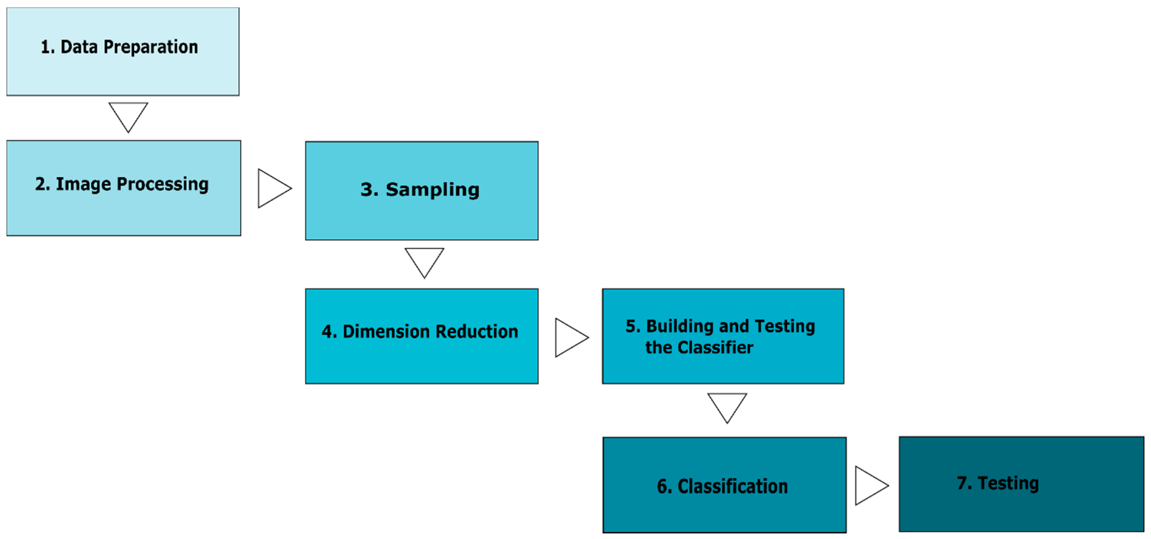
13]. Until recently, inductive predictive modeling using higher resolution data would have been time consuming to the point of redundancy. Protocols presented in this paper attempt to address this using machine-learning techniques, dimension reduction and classification to generate posterior probability maps useful as decision support tools.
The protocols used in this paper are built on earlier research into the use of remotely sensed imagery and statistics to produce probability models. These approaches were used to develop what are termed by Chen at al as ‘Direct Detection Models’ and the history and earlier iterations of this process are described more fully elsewhere [14,15]. Many of these applications have developed over the last two decades to assist federal agencies in the USA to comply with legislation that requires government agencies to account for the impact of publicly funded projects on historic and archaeological sites (National Historic Preservation Act of 1966: Section 106), and to be responsible for the management and preservation of these sites (National Historic Preservation Act of 1966: Section 110). Similar frameworks like the European Landscape Convention, which requires signatories to identify and assess significant changes within their cultural landscapes (ELC 6: C 2000), lay a foundation for identifying and cataloguing sites within a European context. In both cases, the inventorying and recording of archaeological sites are crucial to their management and preservation. Traditional survey techniques are expensive and require considerable time. Direct detection models were developed to assist this process through the statistical analysis of data from a wide variety of sources, most saliently that of imagery. These datasets come from a range of sensors including synthetic aperture radar (SAR) and hyper and multispectral data [16,17,18]. In using multispectral data, direct detection models are ideal for identifying non-extant sites or sites with very subtle surface signatures. Early models used frequentist statistics to establish relationships between sites and background datasets [16]. A detection model developed for San Clemente Island, California, used data which included a high-resolution DEM derived from polarized synthetic aperture radar (SAR) data collected by the JPL/NASA AirSAR platform (C-, L-, and P-Band), polarized X-Band SAR data collected by the GeoSAR platform (developed by JPL/NASA for use by the private sector), NDVI and Tasseled Cap indices derived from 4-band IKONOS satellite multispectral imagery, and digital elevation models generated from AirSAR C-band data and GeoSAR X-band data. Points were randomly seeded away from known archaeological sites and these points acted as non-sites. Overall, individual Student’s t-tests were performed on the mean site and non-site values from 11 datasets. From these 11, four were repeatedly significant, and a predictive model was constructed using the best performing thresholds of each dataset. Models were tested by means of a Gain Statistic, which compares the ratio between the percentage of total study area within each probability, and the percentage of correctly identified sites [19]. The model produced gain statistics between 90 and 99.81; however, the very high gain statistics were calculated from small area percentages. Recent advances in computational capacity have allowed the use of statistical learning techniques. These methods allow a far greater dimensionality of data and for more data to be utilized simultaneously; however, it should be noted that more data does not automatically equate to better models. Higher dimensionality can results in over-fitting, and the ability to understand causal relationships can be lost. Chen et al. presented a direct detection model for Fort Irwin that included many protocols employed in this paper, including band difference ratios and principal components analysis. They were using site data represented as points and so employed a multi-ring annuli sampling approach which resulted in very high dimensionality (where d = 2160). Classification used a linear discriminant analysis with a Bayes plug-in classifier. This assumes class conditional normal distributions with the same covariance matrices. Results (as plotted on ROC curves) were promising but producing a usable probability map was time-consuming given the large number of dimensions [14,15].
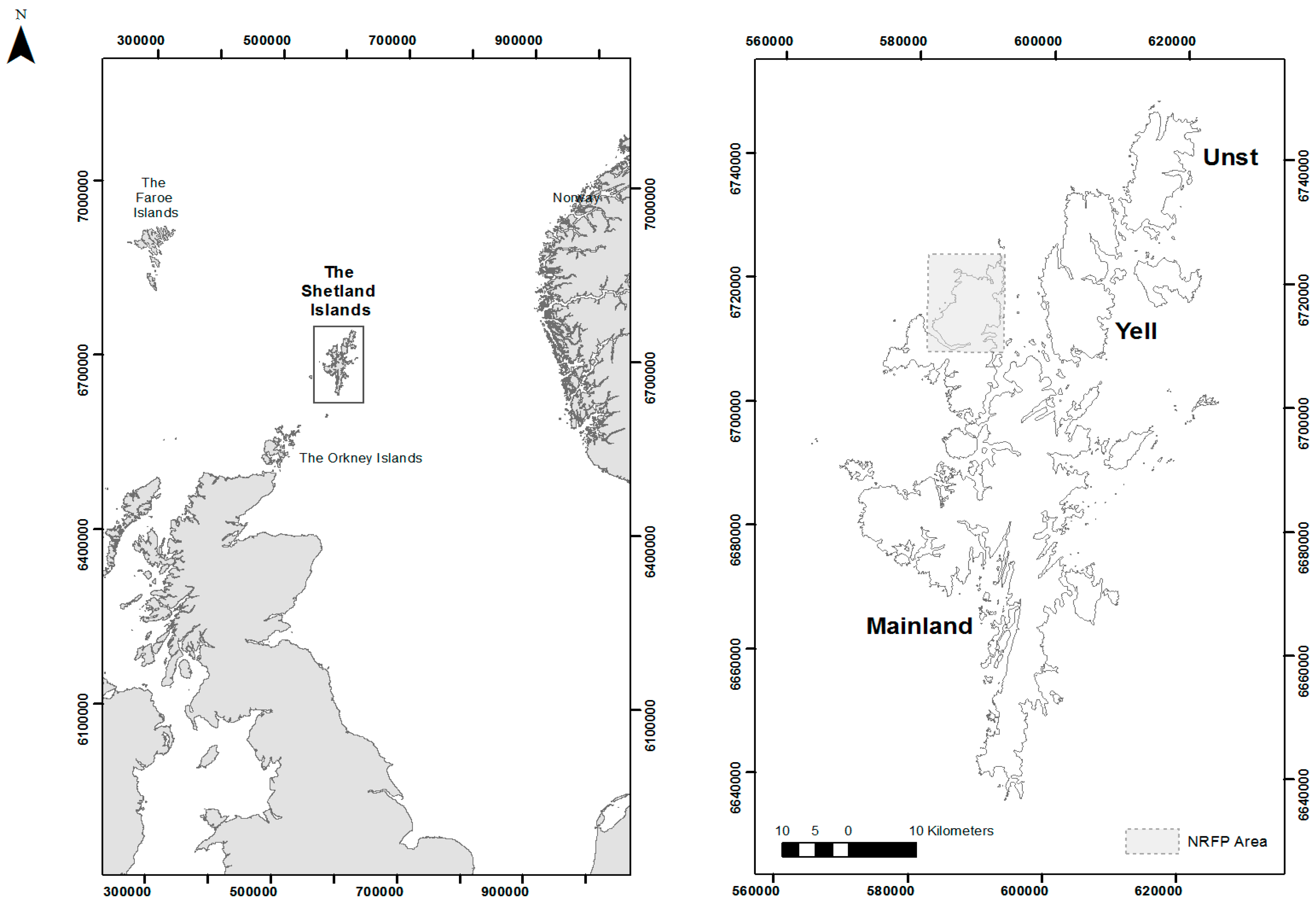
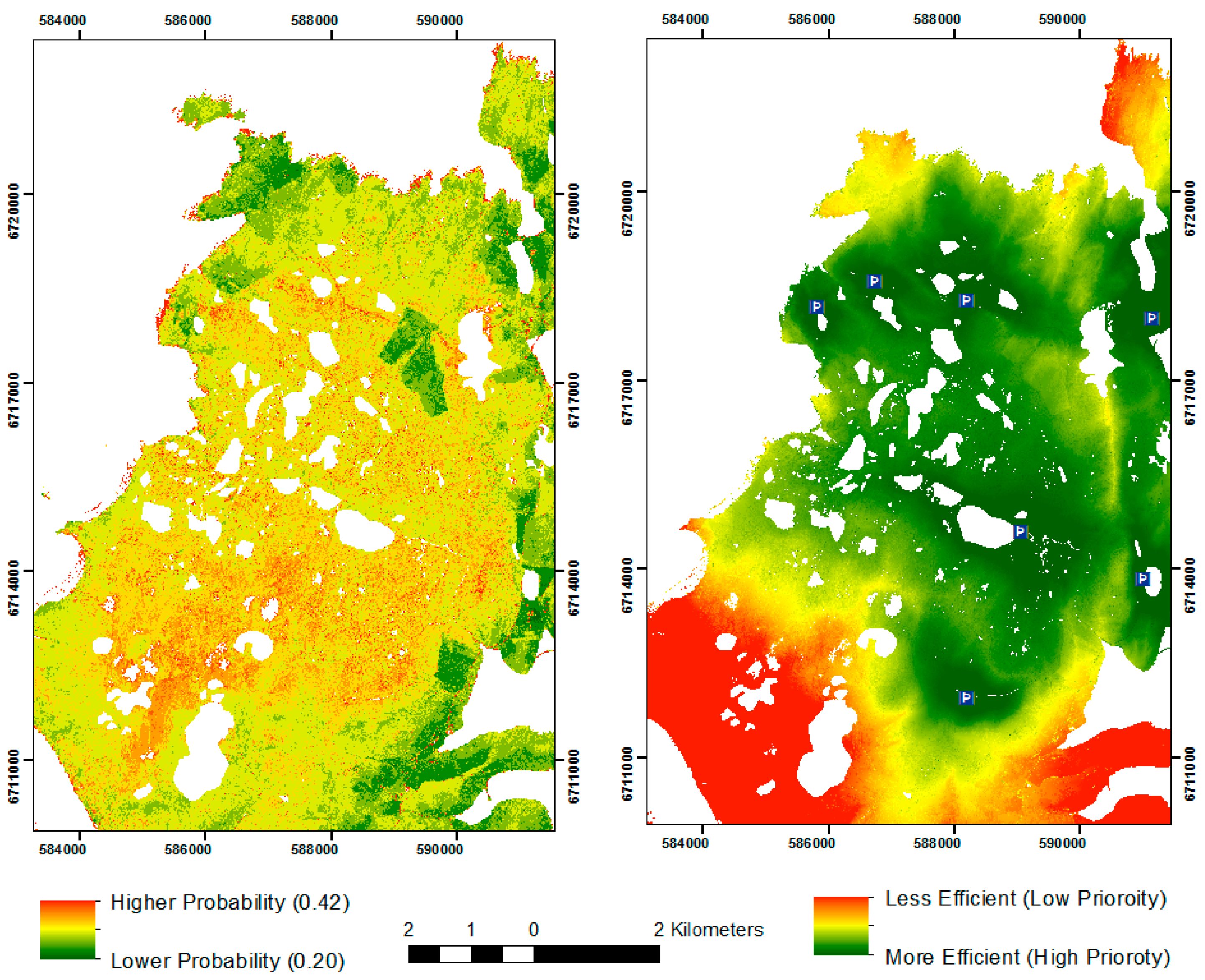
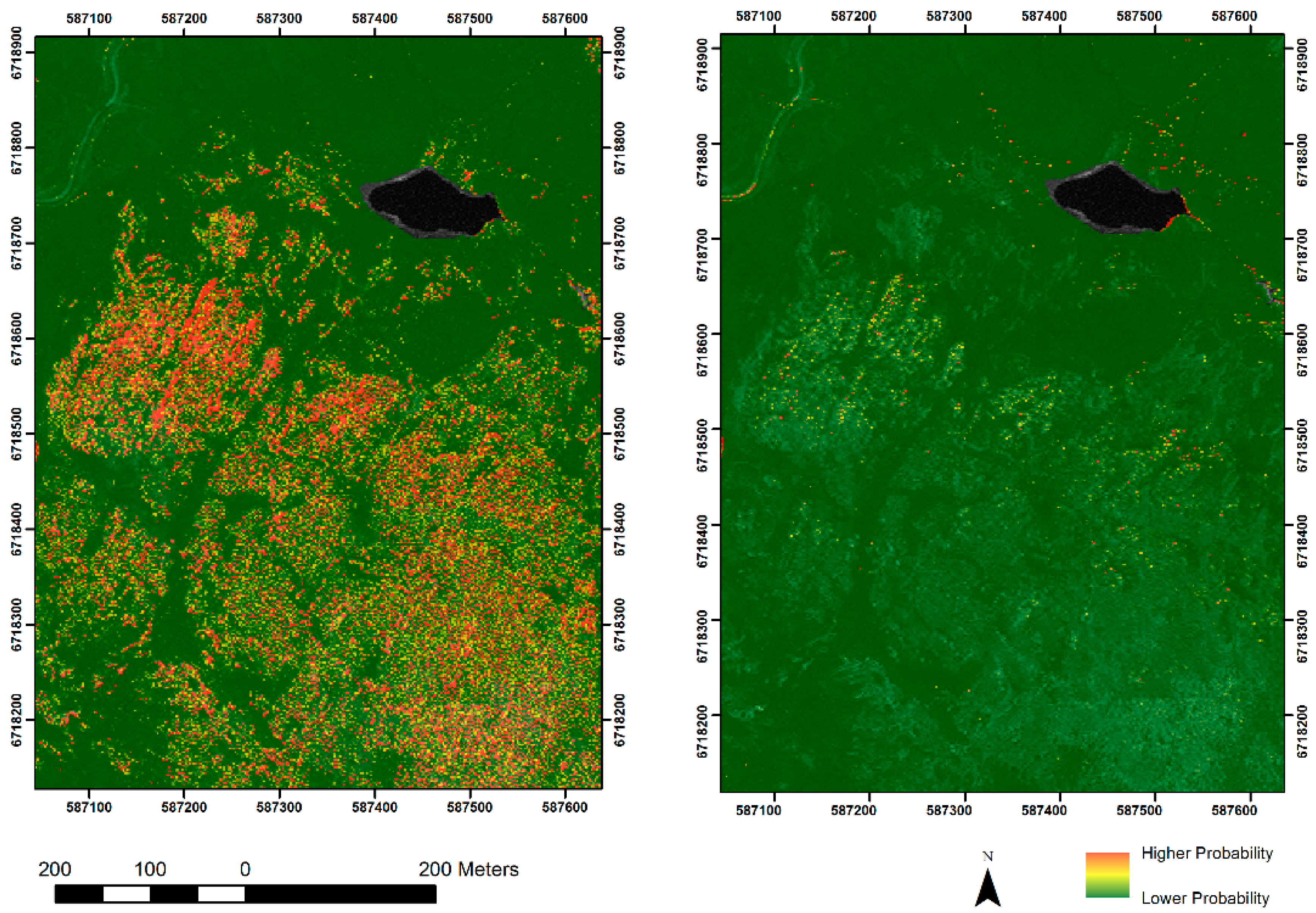
As aforementioned, intemperate weather coupled with the isolated nature of the sites mean only 20% of the NRFP landscape has been surveyed in two survey seasons. This represents an actual value of less than 25 km2. There was a need to more efficiently focus resources, and it was hoped that a survey cost-efficacy model could be generated using a probability model created from Worldview-2 imagery and other topographical data, and a least-cost model which records actual movement costs through the modern landscape. Many dykes are less than 2 m in width so it was hoped that the higher resolution of WV-2 could enable identification at a finer scale. The protocols and applications presented in this paper build on protocols developed for direct detection modeling, but favor a linear discriminant analysis (LDA) classification approach to the frequentist approaches and Boolean merges used in earlier iterations [16,17,
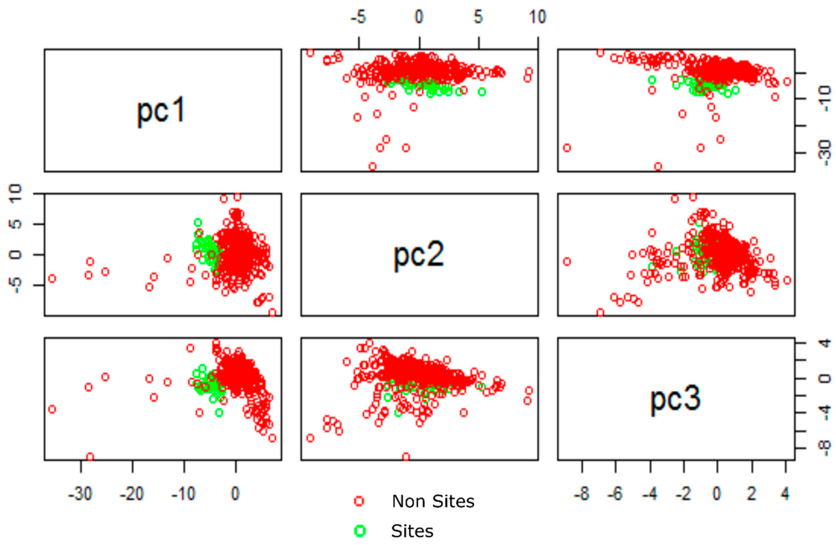
18]. They also use principal components analysis (PCA) to reduce redundancy rather than assessing relevance using a Students t-test.

2.2. Project Datasets

Launched in October 2009, the Worldview-2 satellite sensor provides 0.46 m panchromatic, and 1.84 m multispectral imagery in 8 color bands ranging between lower coastal blue and upper near-infrared (Table 1). The sensor was launched and is operated by DigitalGlobe and imagery for the project was provided free-of-charge through the DigitalGlobe Foundation. The data awarded were acquired on the 3 May 2011 and covered an area of 970 km2, the majority of which (585 km2) covers the sea. There was some cloud cover (0.004%), which cast dark shadows. Multispectral (MS) imagery is ideally suited to the Shetland landscape where sharp contrasts exist between geologies and land-use. The color contrast between the blue felsite and the red granite bedrock is particularly striking and is the basis for the sampling components of this paper. The project geodatabase also contains more traditional digital data sources including a 5 m elevation model obtained through the Ordnance Survey UK.
As discussed in Section 1.2, the extents of 45 workshops were surveyed using differential GPS. These known sites ranged in size between 8 and 278 m2 and were used to train the classifier. 393 known non-sites were also generated. This was the maximum possible number of points based on certain criteria: they had to be within the 20% of the surveyed landscape (to ensure that they were definitive non-sites), they had to be more than 100 m apart, could not be within 100 m of a known site and could not be in parts of the imagery covered by cloud, shadow or water. It was important that known non-sites shared similar dimensions to known sites and so points were buffered to provide extents proportionally based on the extents of known sites. For example, 52% of known sites had extents between 5 m2 and 10 m2 so 1.8 m buffers were generated randomly around the same proportion of known non-sites (the area or circle with r 1.8 m is 10.18 m2). Locations of felsite outcrops recorded during regional survey were available for testing. Most of these points were not archaeological sites; however they recorded the definitive locations of felsite in the landscape.

2.3. Image Processing Techniques

Level 2A Worldview-2 data provided by the Digitalglobe Foundation was already radiometrically and sensor corrected, projected and georeferenced based on a coarse global DEM. Data was further corrected using the Quick Atmospheric Correction (QUAC) tool [19]. Worldview-2 imagery can be used to generate band combinations and spectral indices that are linear combinations of two or more wavelengths highlighting specific features in the imagery. Examples include vegetation indices which record crop yields or chlorophyll content and are calculated using visible red and red-edge bands, which represent the point of sharpest change in the spectral curve (around 700 nm) [20,21,22]. The Normalized Difference Vegetation Index (NDVI) is a band difference ratio (BDR) which records plant health by exploring the differences between the red and red-edge. This can be written as:
B i j = b i b j b i + b j   ,     i > j
where bi is the red-edge band and bj is the visible red band. While such BDR do not contain new data, they are useful for exploring the spectral difference of features in the imagery and have been used by Chen et al. in earlier predictive models [15]. BDR are also useful to provide robustness against changes in lighting conditions which, while not essential in this study, can be very valuable when using different datasets captured at different times [14,15]. After Marchisio et al. [23], BDR were undertaken for each band pairing of WV-2 imagery. In total, 28 BDR were generated.
Three topographic derivatives were processed from the five meter United Kingdom Ordnance Survey digital elevation model. During survey, it was noted that workshops tended to be situated at steeper gradients where dykes were exposed on the hillsides. To account for this, a slope relief map was generated which recorded degrees between 0° and 90°. Similarly workshops were predominantly located on north and east facing slopes so a scaled aspect map was generated which linearized the data using its sine. The elevated situation of known workshops afforded wide-ranging views of the landscape. A number of derivative surfaces record topographical or visual dominance including total or near total viewshed and Llobera’s prominence model which records the localized elevation difference within a set radius [24]. For this study, a skyview factor was generated to explore the proportion of the sky visible from a certain point over a 100 m radius [25,26]. This model is usually used with airborne laser scanning data but is used here to identify parts of the landscape that are locally prominent, reflecting a belief by surveyors that this may have been a valid factor in workshop site situation. The MATLAB scripts used in this study require consistent resolution so topographical datasets were re-sampled to 2 m using a nearest neighbor technique. Datasets are listed in Table 2.

2.4. Image Classification

Classification is about assigning observations to different classes, using known responses to assign probabilities rather than binary results. In remote sensing, this process involves assigning each pixel in an image into a specific landscape coverage class. These tools offer an easy and out-of-the-box means of classifying the landscape based on probability values for each class. For this study, a custom LDA classifier was built in the MATLAB program. This had two preparatory steps (discussed above) and five primary steps (Figure 3): Sampling, Principal Components Analysis and Dimension Reduction, Building a Classifier, Classification and Testing the Posterior Probability Model.
Two central tendency statistics, the mean and the median, were sampled from each dataset. The former has been extensively used in earlier DDM modeling, while later was sampled to account for potential skewness of the sites. Ten models were generated based on the statistics sampled from known sites and known non-sites. These are listed in Table 3.
There was bound to be considerable redundancy when such a large number of dataset are used. Doneus et al. explored this issue when using hyperspectral imagery for archaeological prospection and developed a special toolbox to reduce the many the hundreds of spectral bands to only a few relevant layers [20,27]. In this study a standardized principal components analysis (PCA) was used to generate new components. This technique rotates existing values, while maintaining the variance crucial to classification. The first component contains as much of the variability in the data as possible while the second and subsequent components contain increasingly less. It should be stated that PCA only restructures this variance based on coefficients or loadings. This restructuring may be significant to the analyst and provide useful new components where data can be shown to cluster (Figure 4); however, it is possible for PCA to disregard data that might be important. As PCA is a data reduction technique, later components are usually disregarded and these can (in rare cases) contain useful information [28]. This often happens when datasets are not correlated. PCA can also provide a means of assessing the amount of variance in each new component, and the significance of each dataset within each component. This will be discussed in later sections. PCA was used on all models and scree plots based on latent values were used to assess the optimal number of components used to train our classifiers. All classifiers used three or less components. Models that used only imagery and band difference ratios used less components than those which included topographical datasets.
The LDA classifiers were built using known sites and known non-sites using prior probability values of 0.5. As an intermediate step, the two classifiers were tested using leave-one-out cross validation (LOOCV). Rather than partitioning the data for testing purposes, LOOCV is an iterative process which uses only a single value for validation and uses all others for training [29]. This process is then repeated for all values. True positive rates were plotted against the false positive rates on a Receiver Operating Characteristic (ROC) curve (Figure 5). Area under the curve (AUC) is a statistic that computes the area under the curve as a good means of assessing the relationship between true positive rates and false positive rates. It should be stressed that while LOOCV and ROC curves can inform us about the sensitivity and specificity of the classifier, they do not directly test the efficacy of the posterior probability map, which will be explored later in the results section of this paper. This testing method does however allow us to assess the classifier prior to generating the time-consuming posterior probability map. AUC values for models generated in this study are presented in Table 4.
After the classifier was built and tested, it was applied to every cell in the landscape. This time-consuming process was parallelized and run on multiple cores. Pixel values and Worldview-2 BDR were generated for the entire region, and then multiplied by the PCA loadings. The top components were then fed into the classifier and the posterior probability (the probability that a cell belongs to the known sites class) was assessed for each cell. Once the posterior probability model was finished, areas covered by cloud, shadow and water were removed.

2.5. Understanding Access: The Least-Cost Approach

Alongside weather, terrain is a major hindrance to field survey in the NRFP. Accessing more remote parts of the landscape is more time-consuming. There are few roads or tracks, and survey teams must often hike many miles over bog and exposed granite to reach more remote areas. While a posterior probability map would be useful to more effectively target survey, surveying high probability areas in hard-to-reach parts of the landscape is considerably more labor intensive than surveying similar areas which are easier to access. By using a least-cost surface, which calculates a cumulative temporal cost for accessing each part of the landscape, alongside a probability model, it was hoped to generate a hybrid surface that would greater facilitate survey planning. This surface would balance the costs associated with access against the probabilities generated by the models. An anisotropic cost surface (r.walk) was generated in the GRASS GIS program based on physiological factors calculated by Langmuir [30]. Appropriately, these costs were calculated for the Scottish landscape. This surface was generated from carpark locations used during survey, and records costs based on journey time in seconds. Crucially, it accounts for the differences associated with walking both up and downslope. A hybrid model was generated where posterior probabilities were converted to percentage values and scaled according to least cost values. This resulted in a survey planning model or survey efficacy model that identified more and less efficient parts of the landscape for survey (Figure 6).

3. Results

3.1. Assessing the Models

Model efficacy was assessed using a two-sided Kolmogorov–Smirnov (KS) testing and by way of a gain statistic [31]. Results are shown in Table 5. The KS test is a nonparametric test that tests a null hypothesis that both samples of sites are drawn from the same distribution. 1000 random sites were seeded away from test sites across the entire landscape and these were used alongside the field survey sites for the KS test. While this statistic can assess the predictive power of the model, it does not take spatial considerations into account. The gain statistic allows us to weigh predictive capability based on the area percentage of probability and is therefore a more robust means of assessing model utility as a decision support tool. It is not ideally suited to assessing posterior probabilities however, as small area percentages can lead to inflated gain statistics. Conversely, narrow probability ranges can result in poorer gain statistics. In this study, minimum probability area percentages were set at 5% however; some statistics, especially from models that included topographical datasets, had to be calculated using larger areas. These are also noted in Table 5.
Principal components analysis generates a number of outputs which can tell us about the sites used in the model. Each component is associated with a percentage of total variance. The first component contains the most variance and subsequent components contain progressively less. Principal components loadings can tell us the weights or influence of individual bands in each component, where larger positive and negative values are of equal importance. These values can be used to identify important datasets in each model.
In total, 10 models were generated and assessed. Two sampling statistics were used separately for each combination of datasets for Models 1 through 8: the mean and the median. The datasets and sampling statistics used are listed in Table 5. Models 1 and 2 use only the Worldview-2 imagery. The KS p-values allows us to reject the null hypothesis for both models with a 0.01 confidence level. The gain statistic indicates that both have prospective capabilities. Probability values ranged between 0.00 and 1.00. Three principal components were used to generate the models. Model 1 principal component 1 contained 95% of the variance from the eight Worldview-2 bands. The highest absolute loadings were near infrared 2 (0.7154), near infrared 1 (0.6241) and red-edge (0.2936). Model 2 principal component 1 also contains 95% of the variance and has very similar loadings (0.7164, 0.6249 and 0.2914). In Models 1 and 2 the infrared bands are providing most of the variance. Models 3 and 4 use the Worldview-2 imagery and the three topography layers: slope, aspect and sky view. Given the performance of Models 1 and 2, it was expected that the addition of the topographical layers would further improve the performance of the model. This was not the case. While p-values indicated significance, performance decreased significantly with gain statistics for both models around 0.5 suggesting little utility. Area percentages for calculating these gains were significantly higher than Models 1 and 2, and the ranges of probability values fell (between 0.01 and 0.63). The principal component variance for Models 3 and 4 was more dispersed (c. 50%, 22% and 10%) with imagery predominating the top two components and topography the third. Loadings for imagery datasets differ from Models 1 and 2 with higher values for green (0.4125/0.4211), yellow (0.4128/0.4127) and red (0.3946/0.3386) in component 1, near infrared 1 (0.5115/0.4918) and 2 (0.4984/0.5021) in component 2, and skyview (0.6926/0.7618) and slope (−0.6921/−0.5997) dominating component 3.
Models 5 (mean) and 6 (median) used only band difference ratios derived from the Worldview-2 bands. KS p-values were high for both models, which also performed well with gain statistics of 0.7877 and 0.7728, respectively. Two principal components were used to generate the models. Probability values ranged between 0.00 and 0.99. Component 1 contained 80% of the variance in Model 5 and 82% in Model 6. Component 2 contained 13% and 14%, respectively. Loadings are more evenly distributed than in Models 1 through 4. In both models, band difference ratios between blue/coastal blue and near infrared 1 and near infrared 2 have the highest loadings. Models 7 (mean) and 8 (median) used the band difference ratios and topographical datasets. Again, the addition of these datasets decreased the performance of the models although not to the same extent as Models 3 and 4. While p-values are higher, gain statistics were larger than Models 3 and 4, although this is likely due to the smaller areas used in their calculation. The range of probability values fell to between 0.01 and 0.14. Principal components variance for the top three components was ca. 60%, 18% and 8%. Again, loadings were quite evenly distributed with highest values in the blue and near infrared band difference ratios. In both models, the variance associated with the topography was in the fourth component and so was largely redundant.
Models 1 through 8 indicate that both the mean and median sampling statistics perform equally well. Models 9, which only used the mean statistic, classifies the landscape using the original Worldview-2 datasets and the band difference ratios. The latter are linear combinations of the original bands and will therefore be strongly correlated; however, band difference ratios will, like a normalized vegetation index, provide an alternate way to explore the same data. This resulted in a far larger number of datasets (8 bands and 28 band difference ratios). Results were very positive, returning the highest gain statistic from all models (0.9365) in a small area (5%). Probabilities ranged between 0.20 and 0.42. Only two principal components were used to create the classifier and these contained 58% and 28% of the variance. Again, the blue/coastal blue and red edge/near infrared band difference ratios dominated component 1 with coastal blue/red edge the largest (0.2164) followed by coastal blue/near infrared 2 (0.2147). Blue (0.2941) and coastal blue (0.2897) were the dominant loadings in component 2.
Model 10 used the same data as Model 9 but also included the topographical datasets. Once again, the topographical models decreased the performance of the model when compared to Model 9; however, it has a significant p-value and higher gain statistic than Models 1 through 8 (0.7850). Probability values ranged between 0.13 and 0.32. The top four principal components contained 54%, 26%, 9% and 4%, however only the top three were used to build the classifier. As with Model 8, the majority of the variance from topographical datasets was captured in the fourth principal component. Again, variance was more evenly distributed than Models 1 and 2. Blue/red edge (0.2163) and coastal blue/red edge (0.2147) were the highest loadings in component 1, while blue (0.2943) and coastal blue (0.2899) and were in the highest in component 2.

3.2. Assessing the Cost-Efficacy of the Study

The majority of models generated in this study had considerable predictive power. They also took considerable time and energy to build and run. Cost-efficacy was assessed by comparing the performance of the models against two other classifiers available in commercial remote sensing packages: maximum likelihood and random forests. Parameters from Model 9 were used in both cases (eight Worldview-2 bands and 28 BDR). The random forests classifier used 1000 trees. The random forest classifier also provides us with feature importances of individual datasets in the classification. This enables variable selection based on importances so a classification was performed using only the top five parameters. A final random forest classification, which explored the dimension reduction capabilities of the classifier was also run using the top five imagery datasets and the topography datasets. Results are shown in Table 6. All five classifiers showed considerable predictive capabilities and the variable section step improved the performance of the random forests model. Interestingly, the addition of the topographical datasets to the random forest classifier again decreased performance. The maximum likelihood and random forest classifiers had higher KS p-values but smaller gain statistics than Model 9.
There is always a risk when using PCA that crucial variance will be captured in later components and disregarded. A comparison of the random forests importances and the PCA loadings suggest this is not the case. The three most important bands in the random forest classification were coastal blue, coastal blue/near infrared 2 band difference ratio and the blue/near infrared 2 band difference ratio. The principal components loadings from Model 9 and the importances from the random forest classification both identify the blue bands and the blue/near infrared bands are the most important.

3.3. Integrating the PPM with Least-Cost Surfaces

The survey least-cost efficacy model scales the posterior probability model based on movement cost functions from carparks in the survey area. In this model, areas of high probability will have lower costs than surrounding areas even when they are some distance from carparks. Lower probability areas far from carparks score the lowest. For example, the high probability areas towards the southwest of the area, near the top of Ronas Hill (Figure 7) have low costs even though they are nearly two hours walk from the nearest carpark. Conversely, areas to the far north and far south of the map have high costs, even though they are close to carparks, due to their low probabilities.

4. Discussion

4.1. Posterior Probability Modelling and Archaeological Field Survey

Models developed using custom classifiers perform stronger than both a maximum likelihood and random forests classifiers. Gain statistics are generally high as are significance levels from KS testing. It should be noted that posterior probability values tend to be lower for the higher dimensional datasets (0.10 < x < 0.40) but these values are relative and have little operational impact when we consider the difference between known sites and known non-sites on a ROC curve. It should also be noted that sampling from covariate datasets like the BDR are usually correlated with other nearby locations. Workshops tend to be clustered resulting in overly optimistic predictions. Future attempts could apply spatial statistics to account for this correlation. Nonetheless, as a standalone model, the posterior probability model is valuable. Its greater utility as a survey decision making support tool is visible when used alongside least-cost models to generate a survey efficacy model. The majority of lowland areas around the lakes towards the center of the study area are deemed low-cost as are the southern and eastern slope of Colafirth Hill around the southernmost carpark. Areas already surveyed during the 2013 and 2014 season are in predominantly low-cost areas reflecting the targeted and largely extensive nature of these seasons. Remaining low cost areas, like those to the center west of the region and south of the southernmost carpark behind Collafirth Hill, have no doubt been avoided as they are difficult to access. The survey efficacy model suggests that these areas are worth exploring.
There can be little doubt that the homogeneity of site type assisted the classifier, which was largely looking for a type of rock rather than the complex range of material associated with some sites. Much like traditional predictive models, uniformity of site type is key for model performance. In more complex areas, one solution would be to break up a dataset into similar sites and generate probability models for each site type, however this would depend on there being both enough sites and that the chemistry and morphology of these sites are correctly recorded. Even with homogenous sites, both commercial and custom classifiers struggle to differentiate between similar rock types at VNIR. This is clear in the Shetlands between felsite and the red granite country rock, which have similar spectral signatures. This naturally raises the question: what are the models actually detecting? It is unlikely that the datasets used in this paper are directly detecting the spectral signature of felsite, which is usually discernable between 1000 and 2500 nm. Worldview-2 only captures data in the visible and near infrared bands between 400 nm and 1040 nm, below the SWIR wavelengths necessary. In this study, it is likely that the classifiers are detecting the direct color of the felsite in the coastal blue and blue bands and associated factors like the lack of vegetation at workshops in the near infrared bands. The NRFP is primarily interested in geology and results would undoubtedly improve with imagery that captured spectra in the SWIR. While the coarser resolution of platforms like ASTER places it beyond our use, the recently launched Worldview-3 satellite captures eight SWIR bands between 1195 nm and 2365 nm. Using hyper-spectral datasets may also address this issue.
AUC statistics suggest that good classifiers do not always equate to good predictive models. All models returned high AUC values yet gain statistics varied considerably. Using a different classifier may improve performance. The LDA classifier used in this study assumes the same covariance for different datasets. LDA was chosen as it is generally preferred for studies with smaller training samples [24]. Quadratic Discriminant Analysis (QDA) assumes that each dataset has its own covariance matrix and so may perform better with a larger number of datasets. It would also allow for the higher variances expected from non-sites. Other high-performance classifiers could also be used. Results would also likely be improved for other areas by addressing sampling. This study uses two sampling statistics: the mean and the mean, both of which are first order measurements, and performed equally well. These statistics were obtained from the surveyed extents of highly homogenous sites. Sampling other statistics, like standard deviations or interquartile ranges, may provide valuable alternate data for classification, especially at more complex sites. Earlier studies by Chen et al. sampled the MAD and mean statistics from a range of annuli however these more detailed approaches were hindered by classification [21]. The MATLAB language used here performs classification using a time-consuming pixel-by-pixel iteration and calculating more complex statistics for the entire region was not possible. Parallelization of the scripts into faster languages will undoubtedly expedite this process and allow more thorough sampling strategies, more suited to complex archaeological sites.

4.2. Imagery and Topography

The PPM generated here used both imagery and topographic datasets. In all cases, the inclusion of topographical data decreased the performance of the models. Where models with topographical datasets performed well, the topography was often relegated to the third or fourth principal component and was therefore redundant. Three potential explanations are explored here. Poor performance may be due to the poor quality of the elevation dataset, which was up-sampled from 5 m to 2 m resolution. Models generated with topographical datasets contained a “tiger-striping” effect on steeper slopes indicative of contour derived elevation data. When Chen et al. used slope at Fort Irwin, the dataset was derived from 1 m resolution airborne laser scanning data and improved results substantially [12]. Better quality data may yield better results in future applications. Secondly, it is possible that topography may not be relevant in site location. This was easily assessed using exploratory statistics on datasets using known site and known non-site locations. A two-sided KS test shows that all bands, with the exception of Worldview-2 green and aspect are significant with a 0.01 level of confidence. The most significant datasets were near infrared 2, near infrared 1, slope and red edge. As such, even the poor quality data should have had predictive benefits. Finally, using PCA on two very different (and un-correlated) types of data might decrease the performance of the components. This is evident in the PCA loadings discussed in the results section. When only imagery was used, the red edge and near infrared bands and band difference ratio loadings are highest. With the inclusion of topographical datasets two things can happen. The loadings either change considerably to green and yellow bands and band difference ratios or the variance from the topographical bands is captured in a lower component and excluded from the model. While PCA may not be an ideal dimension reduction technique, it still performed better than a random forests classification that included both imagery and topography.
While PCA may not be the best tool to use when using two uncorrelated datasets (imagery and topography), it has considerable worth reducing high dimensionality in imagery. The impact of PCA on classification was explored by using the Model 2 datasets to train two classifiers: one with and one without PCA. Results can be seen in Figure 7, which shows probability values for the workshops at the Beorgs of Uyea. The former was generated using three principal components and is substantially less noisy. Interestingly, applying PCA appears to decrease the performance of the classifier (AUC for PCA/ No PCA was 0.9470/0.9730) but increases the performance of the final probability model when assessed using the gain statistic (0.8312/0.6969). The information provided by the loadings is useful when attempting to understand how the classifier is working. In the best performing models, blue and coastal blue bands alongside red and near infrared bands and their band difference ratios had the highest loadings.

4.3. PPM and Scale

Advances in image processing and computational performance enable the application of classification techniques (and posterior probability models) over very large areas. They are also ideal for marginal landscapes where accessibility is difficult. PPM can be tailored to the scale of different landscapes. While the example presented here uses data with a two-meter resolution (after WV-2) coarser resolution datasets could also be used, enabling faster computational processing over larger areas. Performance can also be improved and expanded using parallel processing. This study utilized the Maryland Advanced Research Computing Center (MARCC) high performance computing (HPC) resources, which enabled fast PPM generation. With such resources, the scale and resolution of PPM is potentially unlimited, especially if the code is parallelized into more efficient programming languages.

5. Conclusions

Classification has traditionally been used to assign pixels to landscape coverage classes based on their posterior probabilities. A custom two-class supervised classification technique was presented in this paper that trains a classifier based on known felsite workshops and known non-workshops in the North Mavine region of the Shetland Islands. The posterior probability model generated by the classifier acts as a probability map for these sites, and can be used in a manner similar to a cost-surface to look for sites. This is a valuable tool for developing field survey strategy, especially when coupled with least-cost models which record accessibility. Ten models were generated using different combinations of multispectral imagery and topography, and all but two returned high gain statistics indicating their prospective potential. The two best performing models returned higher gain statistics than probabilities used in both maximum likelihood and random forest classifications.
Posterior probability models represent a versatile and widely applicable tool for site prospection and, when used to support survey, are invaluable decision support tools. The protocols presented in this paper assume homogeneity of site type. They further assume that this congruity will be visible in the spectral returns recorded by sensors. The addition of topography proved less successful than anticipated however this can be attributed to the dimension reduction techniques used prior to the construction of the classifiers. As such, the technique is better applied to datasets like imagery, which are strongly correlated. While classifiers are not directly identifying the geological spectral signatures associated with workshops, they are able to detect and classify associated attributes like lack of vegetation. The necessary homogeneity of sites is a hindrance for more complicated landscapes; however, it may be possible to address this by performing classifications using multiple classes, alternate sampling techniques, or by generating multiple models for a single landscape based on binary classifications.
Remotely sensed imagery has long been an invaluable tool in site prospection, management and protection. By utilizing machine-learning and classification techniques, it is possible to generate posterior probability models over wide areas. These models are based on probabilities, not definitive identification and so bridge a gap between visual and automated site prospection. When utilized correctly, they represent an invaluable decision support tools for field survey.

Acknowledgments

The authors would like to thank the various funding agencies who have enabled this research, specifically: The Irish Research Council who funded the lead author as part of its ELEVATE program (PD/13/15) and covered the costs enabling open access. The NRFP was largely funded by the National Geographic Global Exploration Fund (Northern Europe) Grant Number GEF NE 147 15. Earlier work in direct detection modelling was funded by the US Department of Defense Legacy Program. The authors would also like to thank support from the CSRM Foundation, University College Dublin and The Digital Globe Foundation who provided the imagery used in this study. They would like to acknowledge the resources provided by the Department of Applied Mathematics and Statistics, The Maryland Advanced Computing Cluster (MARCC) and the IDEAS project at Johns Hopkins University. Many people have contributed to this paper through both fieldwork and discussion. Thanks to: The NRFP team: Torben Ballin, David Field, Joanne Gaffney, Bernard Gilhooley, Niamh Kelly, Mik Markham, Brendan O’Neill, Robert Sands, Alison Sheridan and Pete Topping, and to our colleagues at CSRM Baltimore including Bryce Davenport, Jacob A. Comer, Jesse Patsolic and Till Sonnemann. Thanks also to those who commented on drafts of this paper: Percy, G. Li, Youngser Park, Jesse Patsolic and Cencheng Shen. Special acknowledgement is given to Vin Davis who left us in December 2015.

Author Contributions

William P. Megarry performed the analysis and analyzed the data presented in the paper. He undertook the image and data preparation in the GIS and wrote the majority of the scripts for both image processing and classification. Gabriel Cooney conceived, designed and oversaw the field data capture and is principal investigator on the North Roe Felsite Project (NRFP). Douglas C. Comer conceived and designed the direct detection approach using remotely sensed data. He also conceived the idea that PPM could be used as decision support tools. Carey E. Priebe helped conceive and design the Bayesian protocols presented in this paper; specifically the sections on LDA, dimension reduction and machine learning. He also designed the means to test the classifiers using ROC curves.

Conflicts of Interests

The authors declare no conflict of interest.

References

  1. Sheridan, A. Neolithic Shetland: A view from the “mainland”. In The Border of Farming and the Cultural Markers—Short Papers from the Network Meeting in Lerwick, Shetland, September 5th–9th 2011; Mahler, D.L.D., Ed.; Nationalmuseet: Copenhagen, Denmark, 2012; pp. 6–36. [Google Scholar]
  2. Mahler, D.L.D. Farming on the Edge: Cultural Landscapes of the North; Nationalmuseet: Copenhagen, Denmark, 2011. [Google Scholar]
  3. Ballin, T.B. The distribution of worked felsites—Within and outwith neolithic Shetland. In The Border of Farming and the Cultural Markers—Short Papers from the Network Meeting in Lerwick, Shetland, September 5th–9th 2011; Mahler, D.L.D., Ed.; Nationalmuseet: Copenhagen, Denmark, 2012; pp. 62–79. [Google Scholar]
  4. Ballin, T.B. The felsite quarries of North Roes, Shetland—An overview. In Stone Axe Studies III; Davis, V., Edmonds, M., Eds.; Oxbow Books: Oxford, UK, 2011; pp. 121–130. [Google Scholar]
  5. Melton, N.D. Shells, seals and ceramics: An evaluation of a midden at West Voe, Sumburgh, Shetland, 2004–2005. In Mesolithic Horizons: Papers Presented at the Seventh International Conference on the Mesolithic in Europe, Belfast; McCartan, S., Schulting, R., Warren, G., Woodman, P., Eds.; Oxbow Books: Oxford, UK, 2009; pp. 184–189. [Google Scholar]
  6. Ballin, T.B. Felsite axehead reduction—The flow from quarry pit to discard/deposition. In The Border of Farming Shetland and Scandinavia: Neolithic and Bronze Age Farming—Short Papers from the Symposium in Copenhagen, September 19th—21th 2012; Mahler, D.L.D., Ed.; Nationalmuseet: Copenhagen, Denmark, 2013; pp. 73–92. [Google Scholar]
  7. Ballin, T. Making and Island World: Neolithic Shetland. Felsite Polished Axeheads/Adzes and Shetland Knives in Shetland Museum, Characterization and Interpretation of the Collection; UCD School of Archaeology: Dublin, Ireland, 2015. [Google Scholar]
  8. Phemister, J.; Harvey, C.O.; Sabine, P.A. The riebeckite-bearing dikes of Shetland. Mineral. Mag. 1950, 29, 359–373. [Google Scholar] [CrossRef]
  9. Ritchie, R. Stone axeheads and cushion maceheads from Orkney and Shetland: Some similarities and contrasts. In Vessels for the Ancestors: Essays on the Neolithic of Britain and Ireland in Honour of Audrey Henshall; Sharples, N.M., Sheridan, J.A., Eds.; Edinburgh University Press: Edinburgh, UK, 1992; pp. 213–220. [Google Scholar]
  10. Cooney, G.; Ballin, T.; Davis, V.; Sheridan, A.; Megarry, W. Making an Island World: Neolithic Shetland. 2013 Field Season Report; UCD School of Archaeology: Dublin, Ireland, 2013. [Google Scholar]
  11. Practical Applications of GIS for Archaeologists. A Predictive Modeling Kit; Wescott, K.L.; Brandon, R.J. (Eds.) Taylor & Francis: London, UK, 2000.
  12. Harrower, M.J. Methods, concepts and challenges in archaeological site detection. In Mapping Archaeological Landscapes from Space; Comer, D.C., Harrower, M.J., Eds.; Springer: New York, NY, USA, 2013; pp. 213–218. [Google Scholar]
  13. Kvamme, K. Determining empirical relationships between the natural environment and prehistoric site locations. In For Concordance in Archaeological Analysis: Bridging Data Structure, Quantitative Technique, and Theory; Carr, C., Ed.; Westport Publishers: Kansas City, MO, USA, 1985; pp. 208–239. [Google Scholar]
  14. Chen, L.; Priebe, C.E.; Sussman, D.L.; Comer, D.C.; Megarry, W.P.; Tilton, J.C. Enhanced Archaeological Predictive Modelling in Space Archaeology. 2013. Available online: http://arxiv.org/abs/1301.2738 (accessed on 15 January 2016).
  15. Chen, L.; Comer, D.C.; Priebe, C.E.; Sussman, D.; Tilton, J.C. Refinement of a method for identifying probable archaeological sites from remotely sensed data. In Mapping Archaeological Landscapes from Space; Comer, D.C., Harrower, M.J., Eds.; Springer: New York, NY, USA, 2013; pp. 251–258. [Google Scholar]
  16. Comer, D. Institutionalizing Protocols for Wide-Area Inventory of Archaeological Sites by Analysis of Aerial and Satellite Imagery, Project Number (11–158); Department of Defense Program Office: Washington, DC, USA, 2011. [Google Scholar]
  17. Tilton, J.C.; Comer, D.C. Identifying probable archaeological sites on Santa Catalina island, California using SAR and IKONOS data. In Mapping Archaeological Landscapes from Space; Comer, D.C., Harrower, M.J., Eds.; Springer: New York, NY, USA, 2013; pp. 241–249. [Google Scholar]
  18. Comer, D.C.; Blom, R.G. Detection and identification of archaeological sites and features using Synthetic Aperture Radar (SAR) data collected from airborne platforms. In Remote Sensing in Archaeology: Interdisciplinary Contributions To Archaeology; Springer: New York, NY, USA, 2006; pp. 103–136. [Google Scholar]
  19. Bernstein, L.S.; Jin, X.; Gregor, B.; Adler-Golden, S. Quick Atmospheric Correction Code: Algorithm Description and Recent Upgrades. Opt. Eng. 2012, 51, 111719:1–111719:11. [Google Scholar] [CrossRef]
  20. Doneus, M.; Verhoeven, G.; Atzberger, C.; Wess, M.; Ruš, M. New ways to extract archaeological information from hyperspectral pixels. J. Archaeol. Sci. 2014, 52, 84–96. [Google Scholar] [CrossRef]
  21. Horler, D.N.H.; Dockray, M.; Barber, J. The red edge of plant leaf reflectance. Int. J. Remote Sens. 1983, 4. [Google Scholar] [CrossRef]
  22. Verhoeven, G.J.J.; Doneus, M. Balancing on the borderline e a low-cost approach to visualize the red-edge shift for the benefit of aerial archaeology. Archaeol. Prospect. 2011, 18, 267–278. [Google Scholar] [CrossRef]
  23. Marchisio, G.; Padwick, C.; Pacifici, F. Evidence of improved vegetation discrimination and urban mapping using worlview-2 multi-spectral imagery. In Proceedings of the ASPRS 2011 Annual Conference, Milwaukee, WI, USA, 1–5 May 2011.
  24. Llobera, M. Building past landscape perception with GIS: Understanding topographic prominence. J. Archaeol. Sci. 2001, 28, 1005–1014. [Google Scholar] [CrossRef]
  25. Žiga, K.; Klemen, Z.; Oštir, K. Application of sky-view factor for the visualization of historic landscape features in LiDAR-derived relief models. Antiquity 2011, 85, 263–273. [Google Scholar]
  26. Klemen, Z.; Oštir, K.; Žiga, K. Sky-View factor as a relief visualization technique. Remote Sens. 2011, 3, 398–415. [Google Scholar]
  27. Atzberger, C.; Wess, M.; Doneus, M.; Verhoeven, G. ARCTIS—A MATLAB® Toolbox for archaeological imaging spectroscopy. Remote Sens. 2014, 6, 8617–8638. [Google Scholar] [CrossRef] [Green Version]
  28. Traviglia, A. Archaeological usability of hyperspectral images: Successes and failures of image processing techniques. In From Space to Place. Proceedings of the 2nd International Conference on Remote Sensing in Archaeology, CNR, Rome, Italy. December 2–4; Archaeopress: Oxford, UK, 2006; pp. 123–130. [Google Scholar]
  29. Gareth, J.; Witten, D.; Hastie, T.; Tibshirani, R. Classification. In An Introduction to Statistical Learning: With Applications in R; Springer: New York, NY, USA, 2013; pp. 127–168. [Google Scholar]
  30. Langmuir, E. Mountaincraft and Leadership; The Scottish Sports Council/MLTB: Cordee, Leicester, UK, 1984. [Google Scholar]
  31. Kvamme, K.L. Development and testing of quantitative models. In Quantifying the Present and Predicting the Past: Theory, Methods, and Applications of Archaeological Predictive Modeling; Judge, W.J., Sebastian, L., Eds.; US Department of Interior, Bureau of Land Management Service Center: Denver, CO, USA, 1988; pp. 325–428. [Google Scholar]
Figure 1. Northwestern Europe, the Shetland Islands and the North Roe Felsite Project (NRFP) Extent (Images by the Authors).
Remotesensing 08 00529 g001
Figure 2. A Felsite Workshop at the Beorgs of Uyea. Felsite is visible in blue against Red Ronas Granite (Images by the Authors).
Remotesensing 08 00529 g002
Figure 3. Graphical posterior probability model (PPM) generation steps.
Remotesensing 08 00529 g003
Figure 4. Pair Plots for Model 6 components 1, 2 and 3.
Remotesensing 08 00529 g004
Figure 5. Sample receiver operating characteristic (ROC) curve for Model 7 (with area under the curve (AUC) 0.9611.
Remotesensing 08 00529 g005
Figure 6. Probability Model 9 and Hybrid surface using Cost-Surface.
Remotesensing 08 00529 g006
Figure 7. The effects of principal components analysis on 8 Worldview-2 bands, showing workshops at the Beorgs of Uyea.
Remotesensing 08 00529 g007
Table 1. Worldview-2 bands and their wavelengths.
BandLower Band Edge (nm)Upper Band Edge (nm)Centre Wavelength
Coastal Blue396458427
Blue442515478
Green506586546
Yellow584632608
Red624694659
Red Edge699749724
Near Infrared I765901833
Near Infrared II8561043949
Table 2. Datasets for classification.
DatasetNo. BandsSourceResolution
WV-28Digitalglobe Foundation2 m
BDR28Using Data from Digitalglobe Foundation2 m
Slope1Elevation Model from Ordnance Survey2 m *
Skyview1Elevation Model from Ordnance Survey2 m *
Aspect1Elevation Model from Ordnance Survey2 m *
* Resampled from 5 m dataset.
Table 3. Models generated, number of bands, band statistics and datasets.
ModelNo. BandsStatisticDatasets
18MeanWV-2
28MedianWV-2
311MeanWV-2 and Topography
411MedianWV-2 and Topography
528MeanWV-2 BDR
628MedianWV-2 BDR
731MeanWV-2 BDR and Topography
831MedianWV-2 BDR and Topography
936MeanWV-2, WV-2 BDR
1039MeanWV-2, WV-2 BDR and Topography
Table 4. Leave-one-out cross validation (LOOCV) ROC areas under the curve.
Model12345678910
AUC0.95620.94970.95620.95900.95110.95200.96110.95360.05760.9511
Table 5. Model results.
ModelStatisticDatasetsKS p-ValueGainGain Area %
1MeanWV-24.2501 × 10−270.83125%
2MedianWV-21.3669 × 10250.87865%
3MeanWV-2 and Topography0.00100.520238%
4MedianWV-2 and Topography0.00040.530632%
5MeanWV-2 BDR1.7723 × 10−230.86885%
6MedianWV-2 BDR2.5351 × 10−230.87886%
7MeanWV-2 BDR and Topography0.06600.687728%
8MedianWV-2 BDR and Topography0.05900.703925%
9Mean and MedianWV-2 and WV-2 BDR0.00800.93655%
10Mean and MedianWV-2, WV-2 BDR and Topography0.00230.88905%
Table 6. Model 9 Results and Other Classifiers.
ModelKS p-ValueGain Statistic
Model 90.00800.9365
Maximum Likelihood3.6672 × 10−320.8383
Random Forests (1000)1.2831 × 10−050.8438
Random Forests (1000): Top 5 Parameters0.01860.8871
Random Forests (1000): Top 5 Parameters and Topography0.02210.8833

