Evaluating Fourier Cross-Correlation Sub-Pixel Registration in Landsat Images


Geo-Environmental Cartography and Remote Sensing Group, Department of Cartographic Engineering, Geodesy and Photogrammetry, Universitat Politècnica de València, Camí de Vera s/n, 46022 València, Spain
*
Author to whom correspondence should be addressed.
Remote Sens. 2017, 9(10), 1051; https://doi.org/10.3390/rs9101051
Submission received: 14 September 2017
/
Revised: 9 October 2017
/
Accepted: 12 October 2017
/
Published: 16 October 2017
(This article belongs to the Section Remote Sensing Image Processing)
Abstract
:Multi-temporal analysis is one of the main applications of remote sensing, and Landsat imagery has been one of the main resources for many years. However, the moderate spatial resolution (30 m) restricts their use for high precision applications. In this paper, we simulate Landsat scenes to evaluate, by means of an exhaustive number of tests, a subpixel registration process based on phase correlation and the upsampling of the Fourier transform. From a high resolution image (0.5 m), two sets of 121 synthetic images of fixed translations are created to simulate Landsat scenes (30 m). In this sense, the use of the point spread function (PSF) of the Landsat TM (Thematic Mapper) sensor in the downsampling process improves the results compared to those obtained by simple averaging. In the process of obtaining sub-pixel accuracy by upsampling the cross correlation matrix by a certain factor, the limit of improvement is achieved at 0.1 pixels. We show that image size affects the cross correlation results, but for images equal or larger than 100 × 100 pixels similar accuracies are expected. The large dataset used in the tests allows us to describe the intra-pixel distribution of the errors obtained in the registration process and how they follow a waveform instead of random/stochastic behavior. The amplitude of this waveform, representing the highest expected error, is estimated at 1.88 m. Finally, a validation test is performed over a set of sub-pixel shorelines obtained from actual Landsat-5 TM, Landsat-7 ETM+ (Enhanced Thematic Mapper Plus) and Landsat-8 OLI (Operation Land Imager) scenes. The evaluation of the shoreline accuracy with respect to permanent seawalls, before and after the registration, shows the importance of the registering process and serves as a non-synthetic validation test that reinforce previous results.
1. Introduction
Multi-temporal remote sensing analysis aims to extract information from images at different epochs to understand and monitor landscape evolution and to obtain a temporal dimension of natural or anthropogenic phenomena. Multi-temporal analyses are relevant for monitoring environmental processes, such as urban sprawl [1,2], coastline evolution [3,4,5,6], forest dynamics [7], and natural disasters [8].
Depending on the objective, images with different characteristics are required, usually defined by the spatial, radiometric, and spectral resolutions, or the revisit cycle of the satellite platform. Landsat imagery, including TM (Thematic Mapper), ETM+ (Enhanced Thematic Mapper Plus) and OLI (Operation Land Imager), has been a widely used over more than 40 years for multi-temporal analyses due to the long temporal availability and frequency offered (every 16 days since 1984), at least seven multispectral bands available and its medium-resolution (30 m). Its popularity increased due to the free availability announced by USGS (United States Geological Survey) in 2008, fostering the development of multi-temporal studies related to environmental evolution or specific historic events. However, there are limitations when the objective requires finer spatial resolution. Several sub-pixel methods have been developed to handle this limitation and they have been widely applied with different aims, such as soft-classifications and un-mixing analysis [9,10], multi-temporal trend analyses [11], fire monitoring [12] or coastline detection [5,6].
Moreover, those sub-pixel results obtained for each image must be precisely geo-referenced in order to avoid spurious results during multi-temporal studies [13]. When accurate geo-referencing is not available or possible, a precise relative co-registration of the data is required. If the data source is composed of a set of images, the geometric relationships for registering the images to other reference images or data must be found. In [14] the image registration is divided into four basic steps: (1) feature detection; (2) feature matching; (3) transform model estimation; and (4) image resampling. Usually, Ground Control Points (GCP) are detected and matched (steps 1 and 2), and a transformation model is obtained using least squares (step 3). Two main aspects are crucial in image co-registration processes: automation and accuracy. Generally, automation is performed in the feature detection and matching steps [15,16], and accuracy is searched in the model estimation step based on the least squares method. However, the accuracy achieved with the geo-referencing methods based on homologous GCPs mainly depends on the pixel size. Therefore, sub-pixel registration methods must be applied when finer precision than that provided by the image resolution is required.
Other approaches and a variety of methodologies have been developed to obtain automated and robust image registration, such as pyramid images [17,18,19], finding shifts and angle between images from their original and gradient values [20], genetic algorithms [21], taking profit of multi-temporal image series to perform a global image registration [22] or cross correlation (CC) based on the Fourier transform [22,23,24,25,26,27,28,29,30,31,32].
In the CC method, the result is a matrix with the same size of two matched images in which each pixel contains a correlation value. The location of the maximum correlation value gives the x and y offsets. From that basic concept, several refinements are possible. Images at the Fourier domain are composed of two parts: magnitude and phase. The geometric part of the image is represented in the phase part and in some approaches the magnitude part is weighted [33] or is even removed, resulting in a cross correlation but only with the phase and named phase correlation (PC) [26]. Phase correlation is robust to handle radiometric differences between images and the presence of noise, mainly Gaussian [26,30]. Although CC methods are straightforward, fast and robust, they present two main limitations: first, CC only handles translations only along both Cartesian axes of the image; and, second, since the peak is located in a pixel, no sub-pixel precision is directly obtained. Against the first limitation, the improvement of those properties to obtain angle and scale parameters through Fourier–Mellin transform has been tested [24,25]. This paper is focused on the second limitation, the sub-pixel accuracy. When working with medium resolution images, such as Landsat or Sentinel 2, obtaining better accuracy than the nominal pixel size remains a challenge [19,34].
An automatic, fast and robust registering process is suitable to overpass radiometric differences, cloud coverage and SLC-off (Scan Line Corrector) issues of Landsat ETM+ scenes. Phase correlation may be a solution given the mentioned resistance against noise. From that point, sub-pixel accuracy can be achieved using several alternatives: (i) fitting a parabolic function around the correlation peak [30,35]; (ii) computing the ratio between pixel values near the correlation peak [27,28]; or (iii) upsampling of the correlation peak in the Fourier space [23,31]. Trying to choose the most reliable alternative, it has been seen that: (i) The paraboloid fitting around the peak of correlation in [30] is performed using only six images, obtaining 0.1 pixels of error and, in fact, it has been used to register Landsat imagery between bands and with ground control points [35]. However, this may not be an optimal solution given that it was demonstrated that [36] the peak fitting method have systematic errors and, on the other hand, the area surrounding the peak of correlation can be asymmetric [32], being a paraboloid an inappropriate surface to fit. Beside those observations, it can be found [37] that, although the geometric Landsat accuracy has a RMSE lower than 12 meters for nearly 92% of the data, it is not enough for our intentions and a better refinement must be found. (ii) The near-to-peak ratio suggested in [27,28] evaluates only 16 images with errors between 0 and 0.05 pixels. In these tests, the size of the matched images is not specified. In [38], the same previous method is used, obtaining mean errors around 0.7 pixels, but showing heterogeneous results when images from urban, vegetation or desert are used. (iii) The Local Upsampling Factor of the Fourier Transform around Peak of Correlation, named LUFT by [31] and single-step-DFT (Discrete Fourier Transform) by [23], seems to be a more robust sub-pixel georeferencing algorithm because it works without using interpolation or ratios, but with the complete and original spectral information of the image. In [31], authors use LUFT to obtain angles by means of the log-polar transformation of the Fourier transform only to the phase part (phase correlation as we mentioned before), showing great efficiency against noise. In [23], however, cross correlation (not phase correlation) is performed showing an error close to 0. These facts—the resistance against noise of phase correlation and the robustness of LUFT method—make this option suitable for sub-pixel registration of Landsat and Sentinel-2 imagery. However, to ensure the consistency and robustness in different landscapes and conditions present around the world, a rigorous set of tests must be performed and analyzed.
Our main objective is to evaluate the accuracy of the LUFT registration process applied to Landsat TM/ETM+/OLI images and to analyze different methodological factors. Given that no reference translation is available for Landsat images, the accuracy assessment will be performed using two different strategies: by evaluating the translations of a set of synthetic images with known displacements; and by evaluating coastlines obtained at sub-pixel level. The objectives of the first strategy are: firstly, to provide an exhaustive set of numerical results describing the intra-pixel behavior of the registration method, trying to avoid sub-pixel interpolation effects on the synthetic images; and, secondly, to analyze some experimental factors involved in this process, assessing the effects of methodological parameters of the algorithm. In particular, we are interested on the behavior of LUFT when varying the peak upsampling factor, the size of the matched images, the effect of combining different spectral bands, and the effect of the downsampling method used to create the synthetic images with known shifts used for the evaluations. In the second strategy, the objective is to evaluate how the accuracy of sub-pixel shorelines obtained from Landsat imagery improves as the LUFT registration process is applied.
2. Background
In this section, we briefly describe the two algorithms that will be applied in the evaluation tests, the sub-pixel shoreline extraction method and the cross correlation, including some core references where more detailed descriptions are provided.
2.1. Sub-Pixel Shoreline Extraction
This algorithm, tested for Landsat TM/ETM+/OLI images, is based on the absorption of the infrared electromagnetic radiation by water bodies. In a first step, a preliminary coastline is obtained at pixel level by thresholding the processed IR band. The hypothesis is that, around those pixels, there must be the exact location where the land and water spectral behaviors are balanced. Mathematically, this location between land and water corresponds to the inflection point of the curve, or the inflection line in the case of a surface. To locate it, a sub-pixel refinement is done around the preliminary coastline pixels. The image values (DN, digital number) around a neighborhood of those particular pixels are fitted by a function of the form DN = f(x,y), where f(x,y) is the mathematical function that describes the spectral behavior of the near-infrared band in the neighborhood. The final coastline is located with sub-pixel accuracy in the position were the Laplacian operator of this mathematical function equals 0. Further description and application examples of this algorithm can be found in [5,6,39].
2.2. Cross Correlation and LUFT Rationale
Given two images with the same dimensions, the result of applying CC is a matrix with the same dimensions as them where each pixel contains a correlation value. It is expected that the correlation matrix has a peak at the most probable translation offset. Being A and B two vectors or matrices of the same size, Equation (1) calculates the cross correlation between them.
F refers to the direct Fourier transform, F−1 refers to the inverse Fourier transform, and F* indicates the conjugate of the Fourier transform. The phase of an image contains its geometric information and, consequently, phase correlation (PC) provides a more robust solution even varying radiometric conditions between images [22,26,30]. Phase correlation is obtained when the Fourier Transform of each image is divided by its respective magnitude (|F{A}|, |F{B}|):
However, the accuracy of the basic cross correlation and phase correlation is limited by the pixel resolution at integer translations, i.e., the entire pixel where the maximum correlation is located. Different solutions have been adopted to improve accuracy based on the assumption that the correlation peak follows a δ-Dirac [26,27,33]. The selected method, Local Upsampling of the Fourier Transform (LUFT), is described in [23,31]. This method is based on upsampling the correlation peak in the Fourier space. To show how it works, let us assume (Figure 1) that we want to enlarge the size of an image [32]: first, the Fourier transform of the image is computed, which is then embedded into a larger matrix, and, finally, the inverse transform, representing an upsampled version of the original image, is obtained.
The same process is applied to the CC or PC calculation. First, the multiplication in the parenthesis of Equation (2) (see Equation (3)) is performed:
Note that the numerator of Equation (3) obtains the cross power spectrum, while dividing by the magnitudes of A and B obtains the phase of the cross power spectrum [40]. Therefore, the inverse transformation of the numerator would drive to the cross correlation matrix while inverting the whole Equation (3) drives to the phase correlation matrix.
This phase matrix has the same size as the original images A and B. Then, it is embedded into a larger matrix of zeros with the desired resultant size. Finally, the last Fourier inversion is performed with the new matrix, obtaining the upsampled version of the phase correlation matrix.
In terms of computation, the amplified matrix can be too large to work with if great precision is needed (e.g., matching two images of 2000 × 2000 pixels to obtain a resolution of the 20th part of a pixel would imply a correlation matrix of 40,000 × 40,000 pixels). To overcome this problem using LUFT, only a fragment around the peak of correlation is upsampled by matrix multiplication. The upsampling factor (f) refers to the value with which a neighborhood around the CC peak is upsampled. The upsampling factor (f) gives a 1/f definition of that peak—meaning that, for example, when upsampling to double the original image size (f = 2), the peak is located with 0.5 pixels of resolution.
We want to know the optimum configuration and upsampling factor (f) to be applied in our study. If that peak is upsampled indefinitely, would we obtain an ideal translation? Conversely, from which upsampling factor threshold do the results not improve? Since we need common information [40], and considering the influence of landscape [38], which size of the matched images optimizes the results?
3. Materials and Methods
To achieve the proposed objectives by applying the double strategy defined, one the one hand, we need to prepare two data models: a set of synthetic images for testing the maximum possible accuracy, and how some methodological factors can affect this accuracy. On the other hand, two different datasets are needed: the first one is composed of very high-resolution QuickBird images to quantify the expected error associated exclusively to shoreline algorithm, and the other set is composed of shorelines automatically extracted from Landsat images.
3.1. Building Synthetic Images and Designing Registration Test
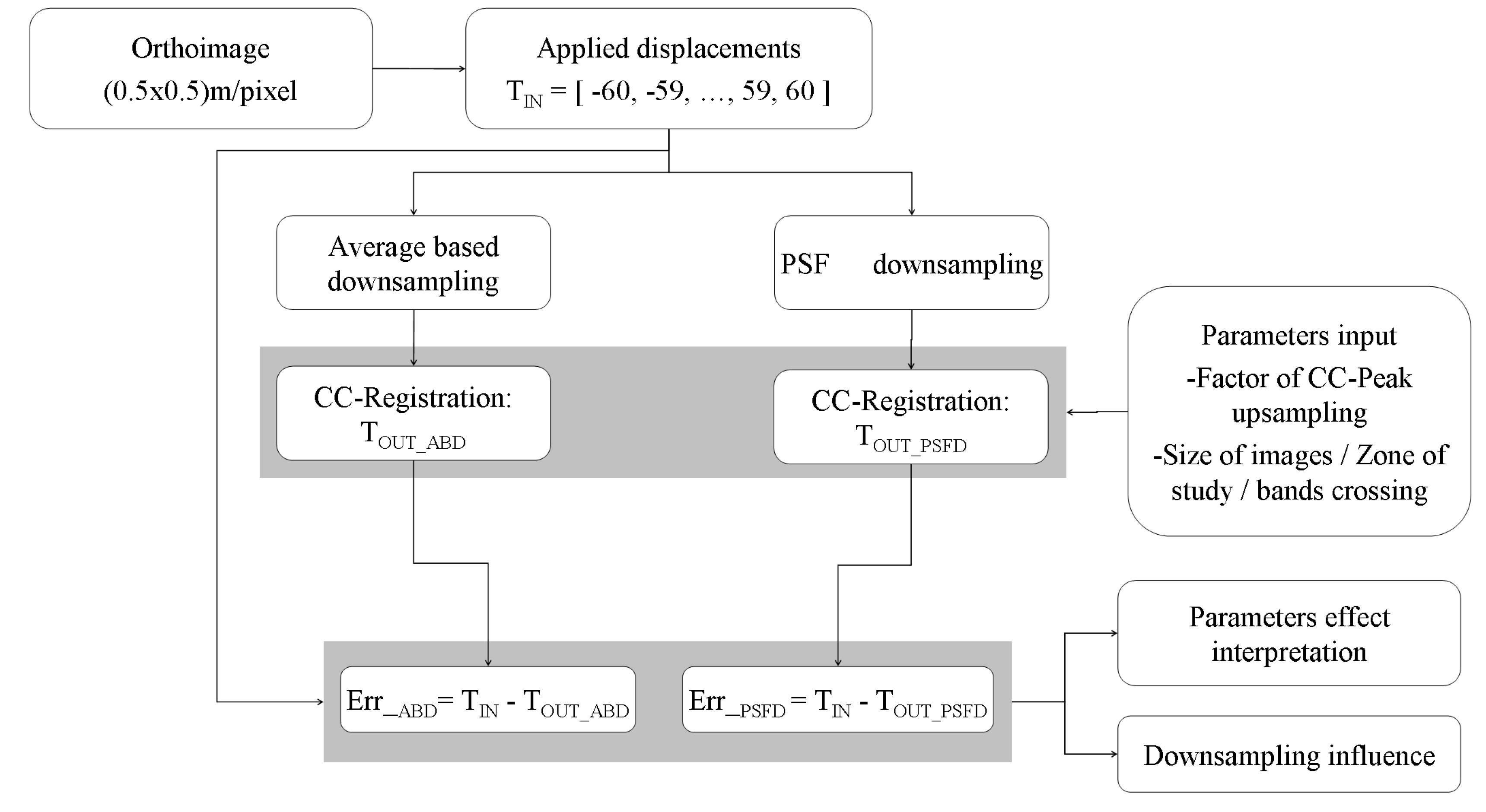
Two sets of 121 downsampled images were generated, where each one had a known translation, serving as a reference (termed TIN) to be compared with the displacement obtained by applying the LUFT method (termed TOUT). Similar to [28], the translations were simulated by downsampling a 0.5 m orthoimage to 30 m. Each simulated 30 m pixel was obtained by averaging 60 × 60 pixel windows from the 0.5 m orthoimage. To create each translated image, the downsampling origin was displaced two pixels (1 m) in the orthoimage along the horizontal (west-to-east) axis. A new independent image is obtained by simulating a satellite sensor acquisition of a new image with its position displaced 1 m. By using this approach, the sub-pixel displacement of each new image is controlled.
As mentioned, two sets of 121 images were created to complete −60 to +60 m (−2 to +2 new pixels) displacements. Each of those two sets of images uses a different downsampling method. The first set is named average based downsampling (ABD set) and follows a standard downsampling procedure, averaging the pixel values of the high-resolution image based on the footprint of each pixel in the low-resolution image. In the second set, a different method was used to create pixels more similar to those from Landsat TM images. In this way, each pixel is weighted in accordance with the point spread function (PSF) of the TM sensor. The description of the Landsat TM sensor specific PSF function is described in [41]. The PSF describes point elements on the terrain are registered by the sensor. Thus, considering a simple 60 × 60 pixels average, the PSF (similar to a Gaussian function) weights each high resolution pixel from the center of the resulting medium-resolution pixel. This description can be used to improve the resolution of images [42] but, in our case, it was used to generate a new set of 121 images, named point spread function downsampling (PSFD).
As shown in the workflow in Figure 2, the CC-registration was applied once the two datasets were created. Considering the obtained value (TOUT) and the reference value (TIN) with which each image was created, the error can be estimated as err = TIN − TOUT. The experimental parameters (factor, image size, and degradation method) were changed as input in the CC-registration step. The effects of each parameter were analyzed after obtaining the errors.
3.1.1. Testing LUFT Upsampling Factor f
The objective of this test was to analyze how the increment of the upsampling factor (f) increases accuracy and from which value there is not further increase. The image at TIN = 0 was used as the reference to register the rest of images, and an image size of 1000 × 1000 pixels was used to ensure a sufficient common surface between matched images. The tested values of f were 1, 2, 3, 4, 5, 6, 7, 8, 9, 10, 11, 12, 13, 14, 15, 20, 30, 40, 50, 60, 70, 80, 90, 100, 200, 300, 400, 500, 600, 700, 800, 900 and 1000. These values should allow us to detect from the original pixel size (factor 1) to the exact 0.001 part of pixel (factor 1000), which represent 30 m and 0.03 m of accuracy, respectively.
In the evaluation, for each of the—known—real (), and the obtained () translations for each factor (f), the error is directly calculated as . Results for ABD and PSFD were obtained and compared.
3.1.2. Testing Matched Images Size
CC is based on the similarity between the matched images. Small images (less information in common) usually perform worse in terms of correlation matching than large images. In addition, depending on the zone used for the registration, translations obtained may vary. Both aspects are related to the overlap area and the type of elements inside it [38,40].
The objective of this test was to analyze the influence of the size of the matched images in the results obtained. Different square dimensions of sub-image sizes were tested (n × n pixels) where n = 4, 6, 8, 10, 12, 14, 16, 18, 20, 40, 60, 80, 100, 200, 300, 400 and 500. Considering that the detected translation can be affected by the type of zone due to different textures or distribution of spatial features, for each tested sub-image size, all possibilities by displacing 10 pixels the origin of the sub-image along the x and y directions were considered, obtaining many different correlation values for each size.
The same evaluation as described before has been applied in this test. In this case, for each sub-image size, several results (along the image where the sub-images were taken from) are available, obtaining the mean () and standard deviation () of the errors.
3.2. Shorelines Obtained from Remote Sensing Imagery to Assess the Performance of the LUFT Algorithm
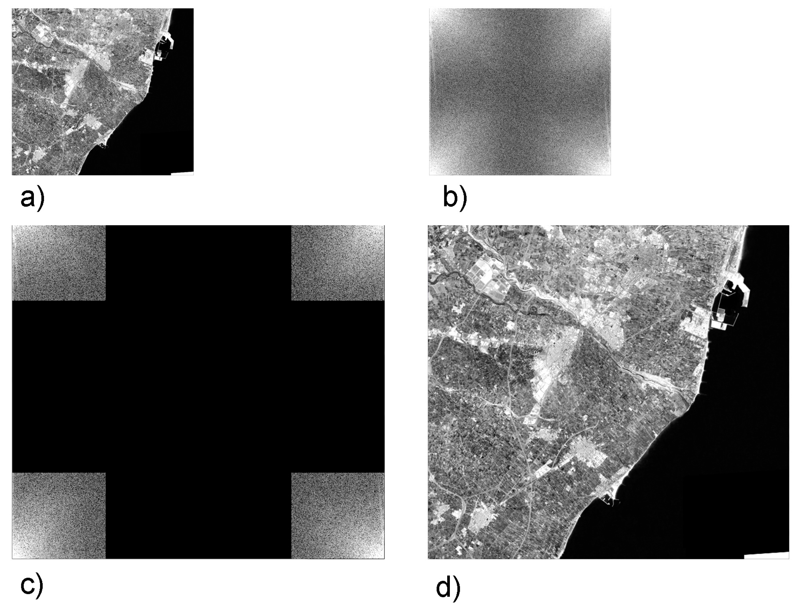
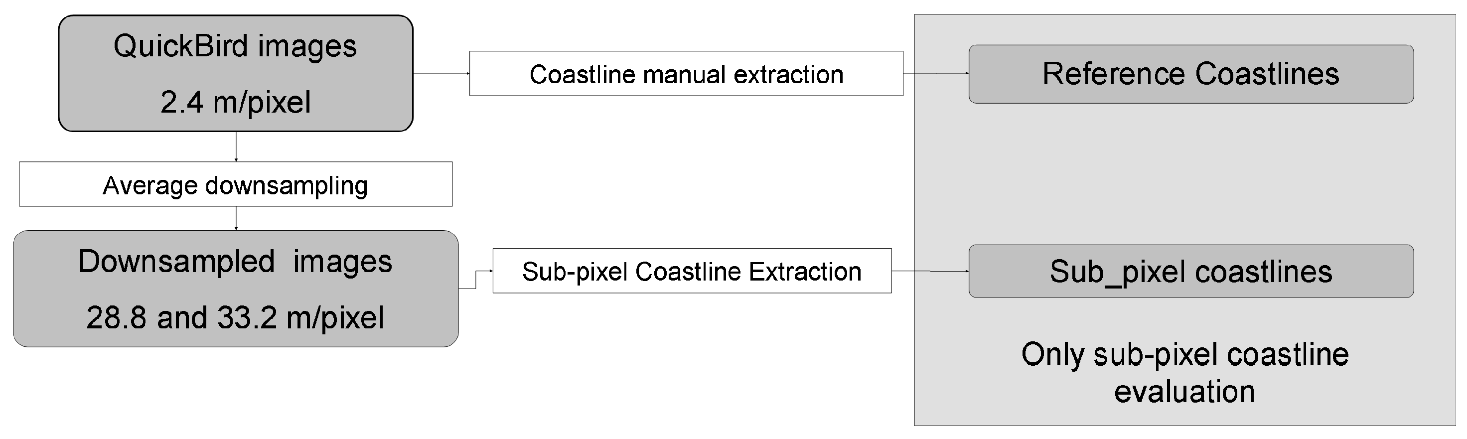
Testing the LUFT method on real application cases is relevant. We assessed how the accuracy of sub-pixel coastlines is improved by sub-pixel registration. To do this, we need to distinguish the two types of errors: the error from the shoreline extraction algorithm and the error of georreferencing the original remote sensing images. To quantify the first error we obtained shorelines from images resampled from very high-resolution images (Figure 3).
Three QuickBird images were used in an independent process [39]. Their original spatial resolution (2.4 m) was downsampled to 28.8 and 33.6 m. The coastline was extracted by photointerpretation of the original highest resolution image to serve as reference or ground truth, and the sub-pixel coastline was automatically extracted from the downsampled version. The coastlines obtained were compared to their respective references to evaluate the errors of the sub-pixel coastlines without considering the influence of the registration process.
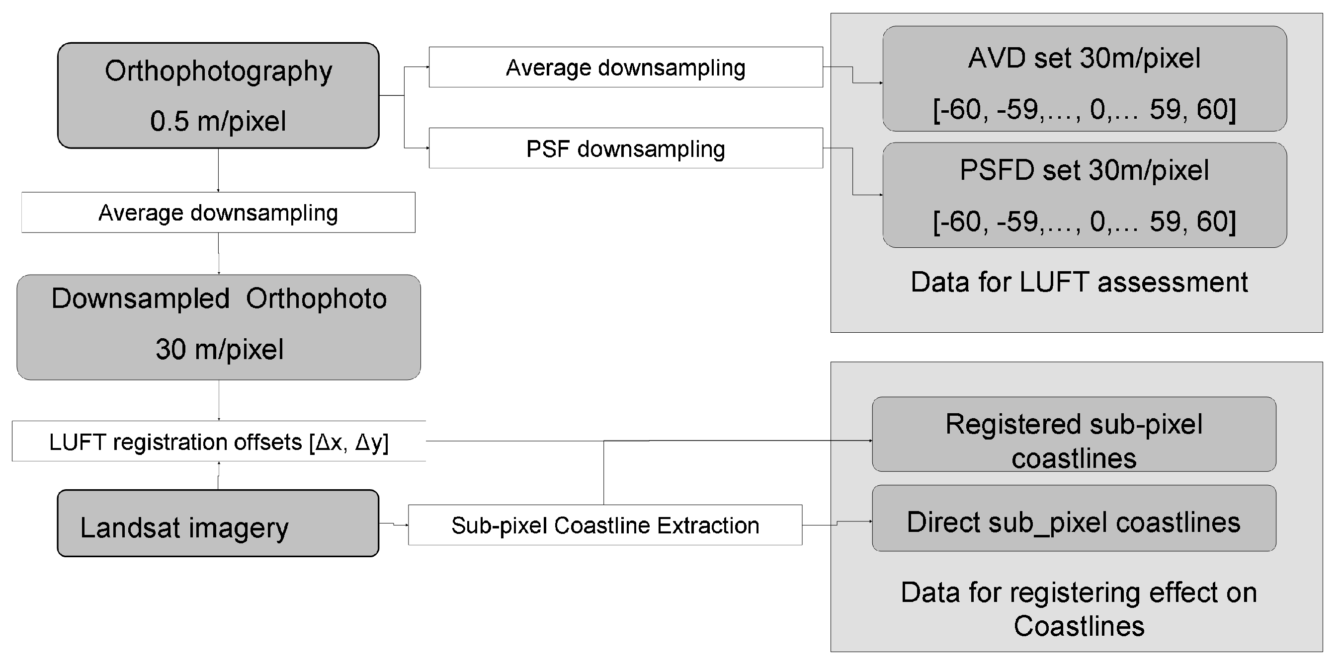
On the other hand, the same method was applied to extract shorelines from a permanent coastal segment obtained from a series of 116 Landsat (TM, ETM+ and OLI) images acquired on different dates. This allowed us to quantify the error obtained both applying and not applying LUFT registration method. A 0.5 m orthoimage of about 19 km east–west and 17 km north–south, located around the area of Castelló de la Plana and Borriana, on the Mediterranean coast of Spain, acquired in the framework of the Spanish National Aerial Orthophotography Programme (Plan Nacional de Ortofotografía Aérea, PNOA, http://pnoa.ign.es/) was used (Figure 4).
As LUFT method requires the matched images to have the same spatial resolution, the orthoimage was downsampled to 30 m to serve as a reference image in the registration of Landsat TM/ETM+/OLI scenes. A total of 59 Landsat TM, 47 Landsat ETM+ and 10 Landsat OLI scenes were used. For each scene, sub-pixel coastlines were extracted from the three main IR bands, and then the offset with respect to the reference image was obtained and applied to the coordinates of the coastlines. Hence, two sets of coastlines, pre- and post-registration, were available. The evaluation of coastlines was made by computing the distance of the points that follow each Landsat image coastline with respect to several permanent seawalls. Pre- and post-registration accuracies should be coherent with the coastline extraction itself and the registration process.
4. Results
4.1. LUFT Accuracy and Influence of Factors
4.1.1. The Upsampling Factor
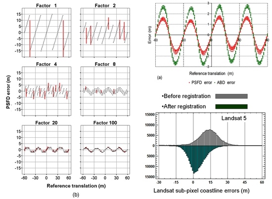
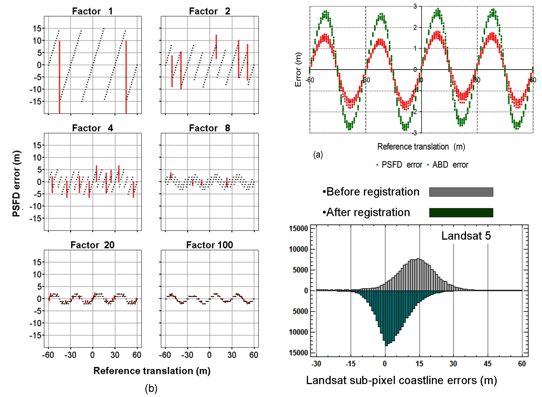
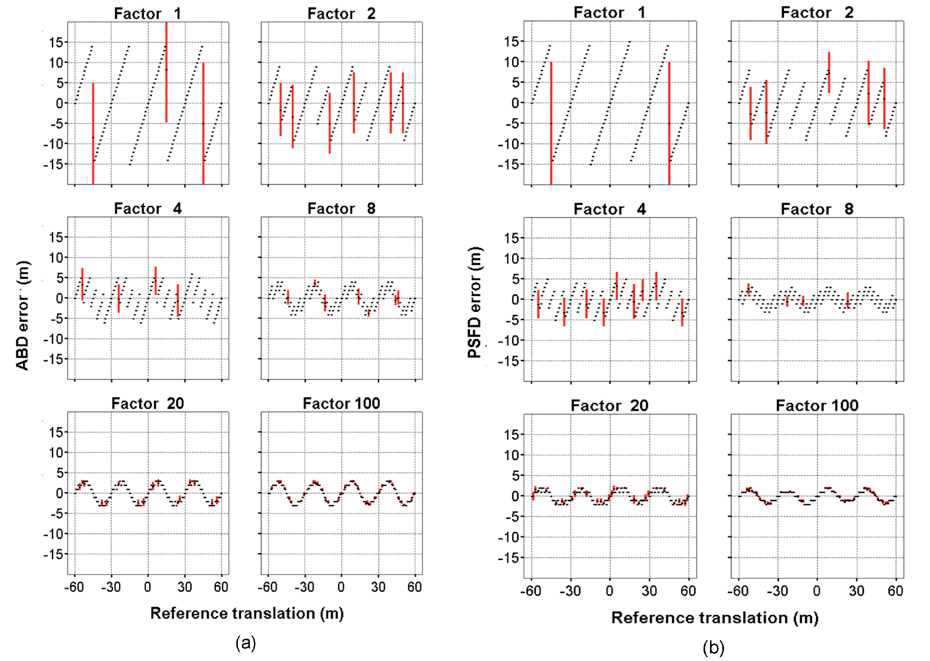
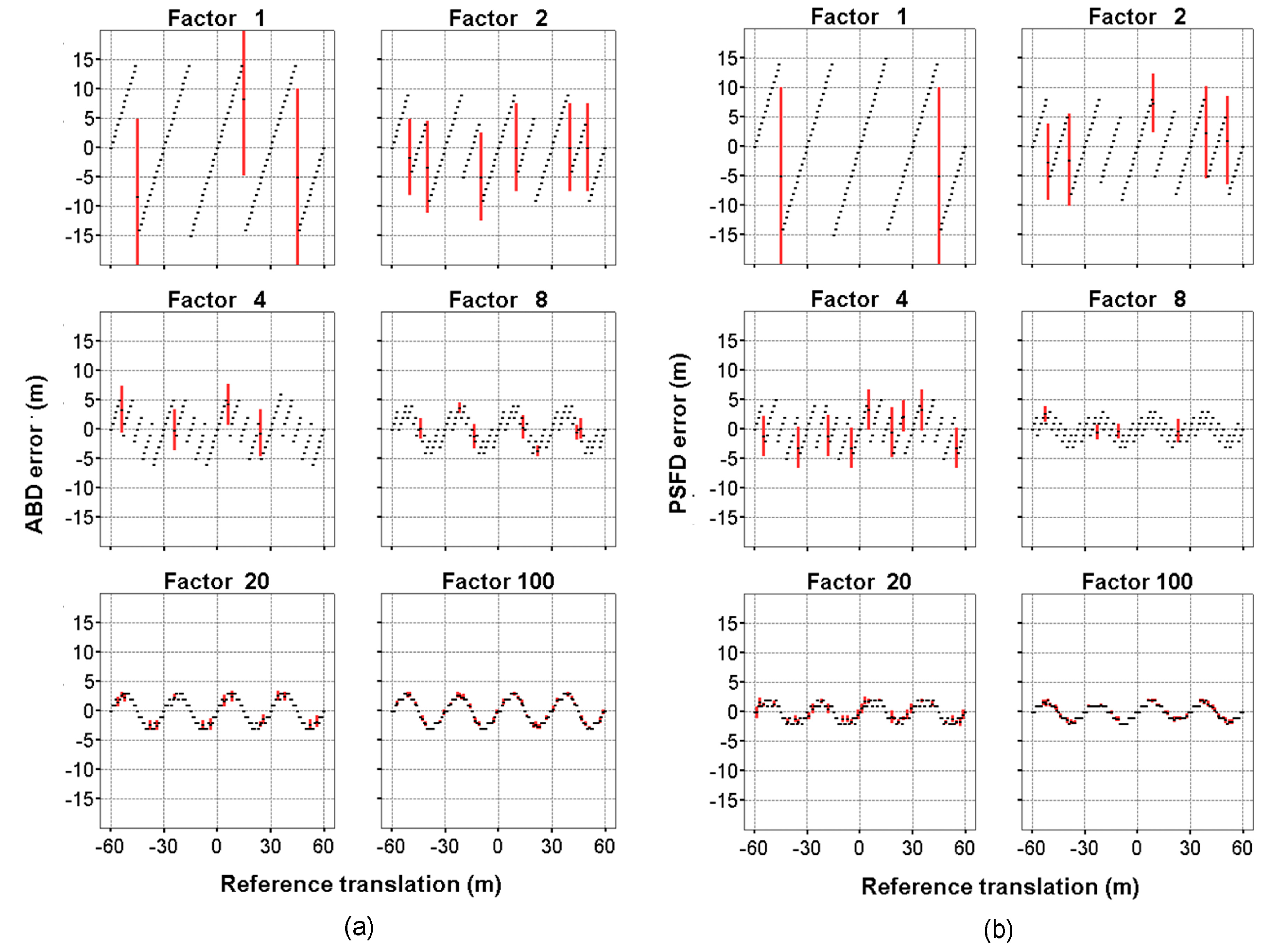
Figure 5 shows the errors at each reference translation for the factors tested. Since each image has three infrared bands and all the possible CC combinations were computed, nine error measures were obtained. The mean of the nine errors (black dots) with their standard deviation (red vertical bar) are represented in Figure 5.
The main remarks of the results are: (i) the meaning of the standard deviation bars is related to the precision of the nine CC for each case, and it dramatically decreases as the f factor increases; (ii) the solution (referring to the actual accuracy obtained) is stabilized from certain factor; and (iii) comparing the errors obtained with the two datasets (differing in the downsampling method used to generate the testing image sets), better results are obtained on the PSFD set than on the ABD method, which shows that the reference data influence the results, and that a great accuracy is expected when applying LUFT on Landsat images.
4.1.2. Image Size and Other Characteristics
The image size test was carried out using an upsampling factor of 1000, ensuring that this parameter did not affect the results. As mentioned in the Methodology Section, for each image size, several sub-images were taken from the original one. Figure 5 shows the results obtained with the ABD set. Analogous results were obtained with the PSFD set and the numerical differences will be described later. The reference translation, TIN, is represented on the horizontal axis. Only some of the used sizes are plotted (sizes = 4, 8, 12, 20, 100 and 500 pixels). Results (Figure 6) demonstrate that matched image size has a relevant influence on the error. Since a minimum of common information is needed to obtain the peak of correlation, larger zones increase the probability of obtaining consistent results. Some types of landscapes with higher frequencies in the images (more differences in the texture of the images) also decrease this minimum image size.
By selecting sub-images in different locations of the original image, many results can be obtained per sub-image size, enabling us to average the value of the detected translation. The mean value () is shown as black dots in Figure 6a, and its standard deviation () is shown as black dots in Figure 6b. Thus, these black dots express how different landscapes affect the LUFT method. Ideally, all the detected translations for each sub-image size should give the same result, but it is not the case. Thus, by having different translations for each sub-image size (s), the influence of the landscapes on the LUFT method was demonstrated, and the robustness of the image size against that effect measured.
4.2. Error in Shoreline Positioning
From two QuickBird images, acquired on 26 October 2004 and 18 July 2005, 25-km-long coastlines were manually digitized. Then, both images were downsampled and the sub-pixel coastlines were extracted. The distances from these sub-pixel lines with respect to their respective reference lines were computed, as well as the mean and RMSE of these distances (Table 1).
The results show that the intrinsic error of the shoreline extraction algorithm, that is, the mean error or offset with respect to shoreline position, is close to zero, but the RMSE approximates to 5 m, depending on the analyzed scene.
Shorelines acquired from Landsat images were analyzed and the errors in their positioning both applying the LUFT registering process and not applying it, measured. To quantify the error, the distances from points that define each shoreline to the actual shoreline position were measured in two segments of 4 km and 2.4 km length completely stabilized by a sea wall.
The coastline locations improved after registration, as expected. The average distance of 76.42 m of unregistered Landsat 5 TM images (Table 2) was due to location errors in the original images. In pixels, this distance corresponds to less than three pixels, but would make some lines unusable. The mean displacement of coastlines after the registration is less than 4 m, and the standard deviations reaches 7 m. This shows that sub-pixel registering process is crucial to take advantage of Landsat images in coastal management applications.
5. Discussion
The results suggest that the LUFT method allows for a fast, automatic and reliable method for sub-pixel registration and multi-temporal analysis of remote sensing imagery. In this section, we will first analyze the influence of different factors in the accuracy of the registration method, then we will discuss the suitability of the LUFT method for real application cases such as shoreline evolution monitoring.
5.1. Factors Affecting Image Registration Accuracy
As expected, considering previous results [23], the LUFT sub-pixel approach is fast and memory efficient. In Figure 5 and Figure 6, the red vertical lines are because the experiment was done using RGB images, so we had results for all the possible pairwise combinations between images, having a total of nine results. Since RGB bands usually present high spectral correlation in terms of landscape reflectance, this parameter has no relevant influence in image registration results.
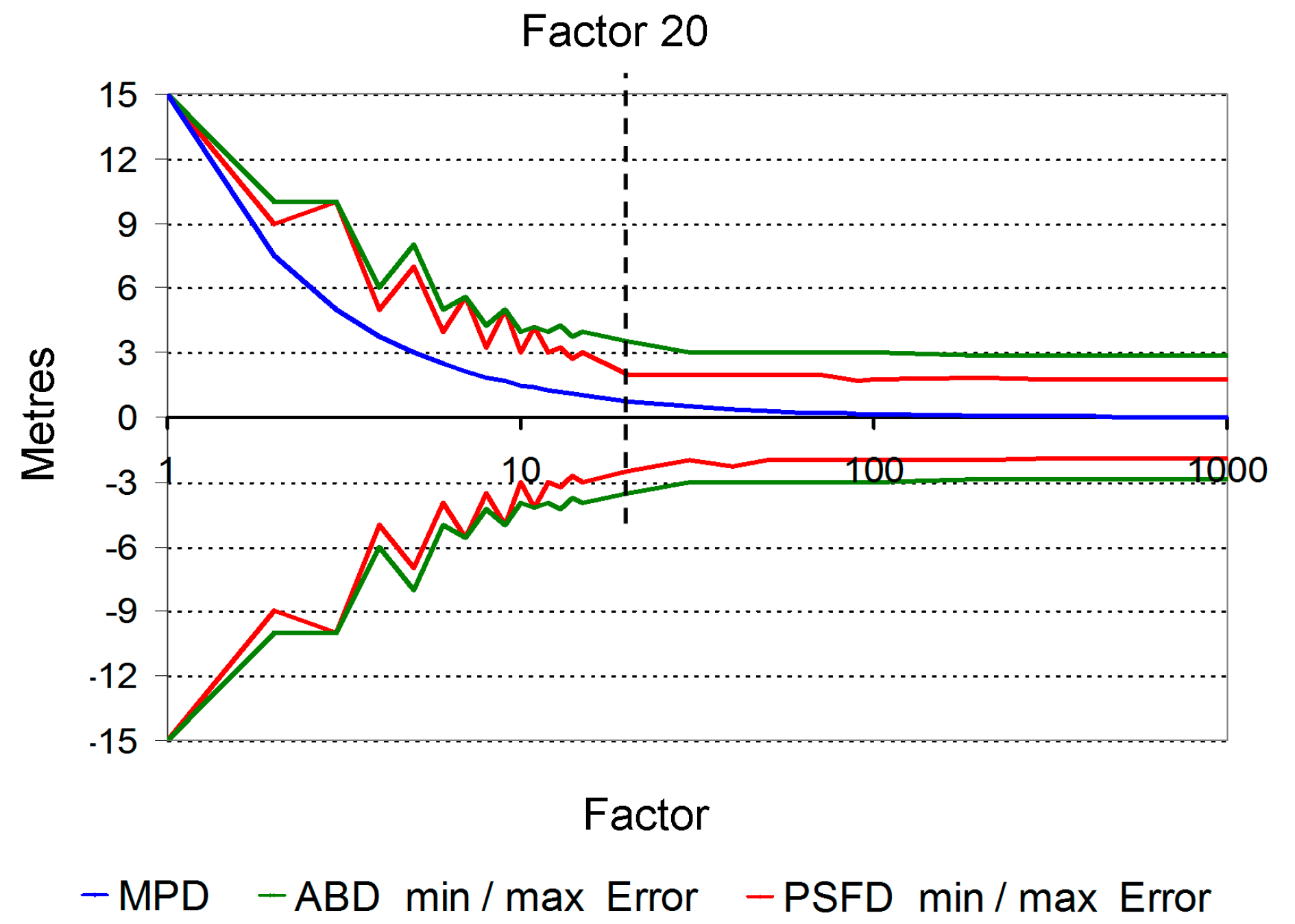
Regarding the upsampling factor, Figure 5 shows how factor f determines the accuracy level obtained using the CC method. As f-factor increases, results improve, but not indefinitely. When using a factor f = 1000, for instance, we observe how the error does not reach what should be expected: a constant 0.03 pixels error. Instead, there is a factor value from which results do not improve, and errors follow a waveform behavior. The minimum and maximum error values are equivalent to the amplitude of the wave. The amplitudes of both image sets (ABD and PSFD) reach a minimum near f = 20 and, from this point, the amplitude does not decrease, even if the upsampling factor increases (Figure 7).
The results show that the different downsampling methods used on each image set have an evident effect on the accuracy. The accuracy stabilizes at ±2.88 m for the ABD image set and at ±1.9 m for the PSFD image set. This difference shows that accuracy is clearly affected by the downsampling method used in each set. Those experimental results agree with the results from other papers, such as in [29], where a Gauss filter was used before downsampling. The PSF function can be considered a Gaussian filter that reduces aliasing. This is probably the reason why the results on the PSFD set are better than simply averaging the images. This was not compared before and it should considered for future tests. Here, the PSF function is used to avoid the aliasing and make images similar to the simulated Landsat scenes.
The second factor to be considered is the image size. Several aspects are related to this factor. CC is expected to draw a δ-Dirac under the assumption that matched images are cyclical or circular [26], i.e., they draw a continuous signal. Normally, this does not occur and the edges of the images get relevance. To face this problem, in [38], the use of windows applied to the original images was proposed to produce a continuous transition between edges, but they also show how the elements in the images could have more actual influence. We did not use any window, although the edge of image may affect the result [24]. Regarding the minimum image size to obtain successful results in our zone, we worked with minimum sizes (e.g., a displacement of 2 pixels with a sub-image size of 4 × 4 pixels) the errors and their standard deviations increase dramatically as the translation increases, due to non-common information, edge effect or lack of circular behavior. As the image size increases, the mean error and standard deviations decrease (Figure 6). However, whereas the standard deviation tends to converge to 0 (e.g., image size 100 × 100 pixels), the stabilization of the mean error follows the abovementioned expected waveform.
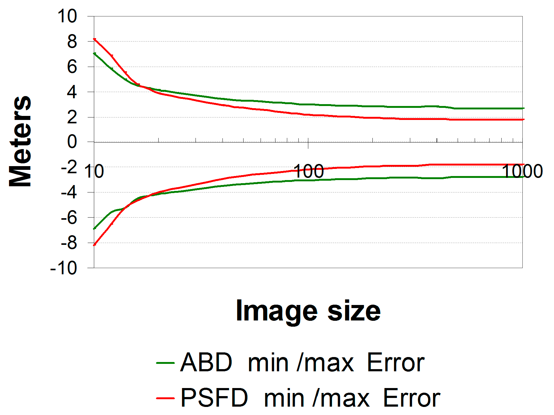
As shown with the upsampling factor, Figure 8 shows the error range for image sizes from 10 × 10 to 1000 × 1000 pixels, and the trend in both image sets (ABD and PSFD) can be compared. From a 100 × 100 pixel image size, accuracies of ±2.88 m in ABD images and ±1.9 m in PSFD images are expected. These values match with the upsampling factor analyses.
Both the upsampling factor and image size parameters have been tested independently. However, the fact that all the solutions are closely matched (low deviations for each reference translation) does not mean that the real displacement is obtained with the same accuracy.
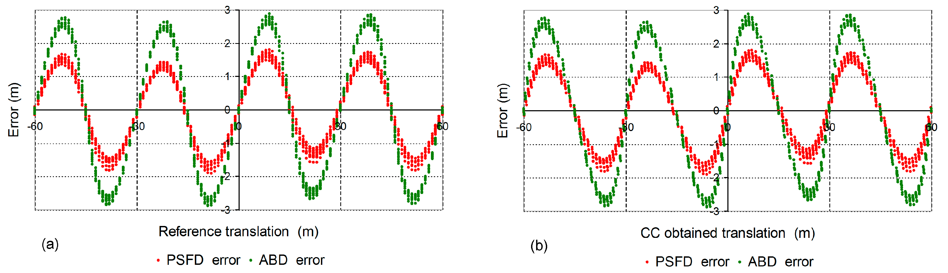
In Figure 5 and Figure 6a, the errors converge to a waveform behavior. Figure 9a shows the errors after applying the best conditions of the upsampling factor (f = 1000) and image size (s = 1000 × 1000 pixels), comparing the use of degradation image sets ABD and PSFD.
The high number of results obtained along the sub-pixel reference translations allows for the analysis of the intra-pixel behavior of the errors (Figure 9). This also shows how these errors cannot be treated stochastically, in terms of standard deviation.
Plots in Figure 9a,b look similar, but they present a significant difference. In real applications, the actual translations are unknown, and so it is not possible to evaluate the committed error from the reference translation (TIN), as plotted in Figure 9a. However, in Figure 9b, the errors are plotted against the obtained translations (TOUT). When applying the CC, the errors are unknown, but, from the near-to-wave behavior, it can be concluded that the sign of the committed error depends on the semi-pixel into which the obtained translation falls. From −0.5 to 0 pixels (−15 to 0 m in Landsat imagery), the errors are negative, but, from 0 to +0.5 (0 to +15 m in Landsat imagery), the errors are positive. The only unknown for real applications is the wave amplitude. This test leads us to conclude that there is a high degree of accuracy when crossing Landsat images (30 m), since simulated PSDF images provide an error in the range of ±1.99 m and the sign of this error is known.
5.2. Applying LUFT to Georeference Shorelines Extracted from Landsat Imagery
This final application of the method helps us to assess the theoretical results in a real case. As mentioned, the final error obtained in shoreline position has two main components: the error associated to the shoreline extraction algorithm (intrinsic error), and the image registration error.
The mean error of the three shorelines obtained from the resampled QuickBird images ranges between −0.82 m and 1.30 m, (Table 1) while Landsat shorelines range between −0.31 m and 3.7 m (Table 2). That difference is less than 0.1 pixel, which is within the bounds of the standard deviations and the range of errors of the registration, so they can be considered equivalent.
On the other hand, the RMSE values of the synthetic shorelines obtained on synthetic QuickBird images range from 4.27 m to 5.76 m, whereas the values from actual shorelines extracted from Landsat images (Table 2) range from 6.33 m to 7.05 m. However, if the amplitude of registration errors (1.99 m for PSFD and 2.88 m for ABD) is considered a deviation, its composition with the shoreline detection on QuickBird comes up to 6.4 m, which is closer to the Landsat shoreline deviations.
Therefore, the combination of synthetic experiments of shoreline extraction and registration are very close to the real application on Landsat imagery, both in average and in deviations. In summary, the results obtained show that LUFT is an adequate tool for image registration at sub-pixel level.
6. Conclusions
Through two different strategies, it has been demonstrated that the use of the LUFT algorithm allows improving the sub-pixel georeferencing process on series of images with Landsat TM/ETM+/OLI resolution. Our tests were focused on the use of Landsat imagery provided by USGS at L1T processing level, which are already georeferenced and LUFT serves as a consistent refinement.
Using the first strategy, two sets of synthetic images were created by downsampling a well georeferenced orthoimage, and the mutual displacement was controlled. The influence of the upsampling factor has been evaluated to obtain optimal accuracy. However, when the upsampling factor (f) is ≥20, the accuracy remains stable and errors follow a waveform behavior.
It has also been shown that a minimum image size is needed to obtain accurate results. LUFT method reaches poor accuracies when the matched images are smaller than 20 × 20 pixels, while the maximum accuracy is obtained for images of 100 × 100 pixels.
The use of two sets of images for the evaluation of LUFT, obtained with different downsampling methods (ABD and PSFD), showed differences in accuracies (±2.88 m for ABD and ±1.9 m for PSFD). This fact shows that the evaluation of sub-pixel processes is affected by the reference data (mainly if this is created synthetically as here). Better results are obtained on PSFD, probably because of the antialiasing effect of the PSF function convolution to create the downsampled images. Since PSF used here tries to reproduce Landsat 5 image behavior, real Landsat images are expected to be accurately registered.
Finally, it has been shown that synthetic results on coastline extraction and registering processes are coherent with their real application on Landsat images. Further tests focused on the detection of the error source, either the registration process or the coastline extraction would help to improve the proposed methods for operational applications.
Acknowledgments
This study has been supported by a research project from the Spanish Ministry of Economy and Competitiveness (CGL2015-69906-R).
Author Contributions
Jaime Almonacid-Caballer, Josep E. Pardo-Pascual and Luis A. Ruiz conceived the work and designed the experiments, analyzed the results and wrote the paper. Jaime Almonacid compiled and prepared the data, performed the experiments and programmed the code.
Conflicts of Interest
The authors declare no conflict of interest.
References
- Yuan, F.; Sawaya, K.; Loeffelholz, B.; Bauer, M. Land cover classification and change analysis of the Twin Cities (Minnesota) Metropolitan Area by multitemporal Landsat remote sensing. Remote Sens. Environ. 2005, 98, 317–328. [Google Scholar] [CrossRef]
- Hermosilla, T.; Ruiz, L.A.; Recio, J.A.; Cambra-López, M. Assessing contextual descriptive features for plot-based classification of urban areas. Landsc. Urban Plan. 2012, 106, 124–137. [Google Scholar] [CrossRef]
- Muslim, A.M.; Foody, G.M.; Atkinson, P.M. Localized soft classification for super resolution mapping of the shoreline. Int. J. Remote Sens. 2006, 27, 2271–2285. [Google Scholar] [CrossRef]
- Muslim, A.M.; Foody, G.M.; Atkinson, P.M. Shoreline mapping from coarse-spatial resolution remote sensing imagery of Seberang. J. Coast. Res. 2007, 23, 1399–1408. [Google Scholar] [CrossRef]
- Ruiz, L.A.; Pardo, J.E.; Almonacid, J.; Rodríguez, B. Coastline automated detection and multi-resolution evaluation using satellite images. In Proceedings of the Coastal Zone 7, Portland, OR, USA, 22–26 July 2007. [Google Scholar]
- Pardo-Pascual, J.E.; Almonacid-Caballer, J.; Ruiz, L.A.; Palomar-Vázquez, J. Automatic extraction of shorelines from Landsat TM and ETM multi-temporal images with subpixel precision. Remote Sens. Environ. 2012, 123, 1–11. [Google Scholar] [CrossRef]
- Brumby, S.P.; Theiler, J.; Bloch, J.J.; Harvey, N.R.; Perkins, S.; Szymanki, J.J.; Young, A.C. Evolving land cover classification algorithms for multi-spectral and multi-temporal imagery. Proc. SPIE Imaging Spectrom. VII 2002, 4480, 120–129. [Google Scholar] [CrossRef]
- Shaikh, A.A.; Gotoh, K.; Tachiiri, K. Multi-temporal analysis of land cover changes in Nagasaki city associated with natural disasters using satellite remote sensing. J. Natl. Disaster Sci. 2005, 27, 9–15. [Google Scholar]
- Busetto, L.; Meroni, M.; Colombo, R. Combining medium and coarse spatial resolution satellite data to improve the estimation of sub-pixel NDVI time series. Remote Sens. Environ. 2008, 112, 118–131. [Google Scholar] [CrossRef]
- Frazier, A.E.; Wang, L. Characterizing spatial patterns of invasive species using sub-pixel classifications. Remote Sens. Environ. 2011, 115, 1997–2007. [Google Scholar] [CrossRef]
- Kennedy, R.E.; Yang, Z.; Cohen, W.B. Detecting trends in forest disturbance and recovery using yearly Landsat time series: 1. LandTrendr—Temporal segmentation algorithms. Remote Sens. Environ. 2010, 114, 2897–2910. [Google Scholar] [CrossRef]
- Kant, Y.; Badarinath, K.V.S. Sub-pixel fire detection using Landsat-TM thermal data. Infrared Phys. Technol. 2002, 43, 383–387. [Google Scholar] [CrossRef]
- Jianyaa, G.; Haiganga, S.; Guoruia, M.; Qiming, Z. A Review of multitemporal remote sensing data change detection algorithms. Proc. ISPRS 2008, 37, 757–762. [Google Scholar] [CrossRef]
- Zitova, B.; Flusser, J. Image registration methods: A survey. Image Vis. Comput. 2003, 21, 977–1000. [Google Scholar] [CrossRef]
- Kenney, C.S.; Manjunath, B.S.; Zuliani, M.; Hewer, G.A.; Nevel, A.V. A Condition Number for Point Matching with Application to Registration and Postregistration Error Estimation. IEEE Trans. Pattern Anal. Mach. Intell. 2003, 25, 1437–1454. [Google Scholar] [CrossRef]
- Netanyahu, N.S.; Le Moigne, J.; Masek, J.G. Georegistration of Landsat data via robust matching of multiresolution features. IEEE Trans. Geosci. Remote Sens. 2004, 42, 1586–1600. [Google Scholar] [CrossRef]
- Hu, A.; Acton, S.T. Morphological pyramid image registration. In Proceedings of the IEEE 4th Southwest Symposium on Image Analysis and Interpretation, Austin, TX, USA, 2–4 April 2000. [Google Scholar]
- Zhang, Z.; Zhang, J.; Uao, M.; Zhang, L. Automatic Registration of Multi-Source Imagery Based on Global Image Matching. Photogramm. Eng. Remote Sens. 2000, 66, 625–629. [Google Scholar]
- Yan, L.; Roy, D.P.; Zhang, H.; Li, J.; Huang, H. An Automated approach for sub-pixel registration of Landsat-8 Operational Land Imager (OLI) and Sentinel-2 Multi Spectral Instrument (MSI) imagery. Remote Sens. 2016, 8, 520. [Google Scholar] [CrossRef]
- Irani, M.; Peleg, S. Improving resolution by image registration. CVGIP Graph. Models Image Process. 1991, 53, 231–239. [Google Scholar] [CrossRef]
- Chalermwat, P.; El-Ghazawi, T.; Le Moigne, J. 2-Phase GA-based image registration on parallel clusters. Future Gener. Comput. Syst. 2001, 17, 467–476. [Google Scholar] [CrossRef]
- Barazzetti, L.; Scaioni, M.; Gianinetto, M. One-to-many registration of Landsat imagery. Int. Arch. Photogramm. Remote Sens. Spatial Inf. Sci. 2013, 40, 37–42. [Google Scholar] [CrossRef]
- Guizar-Sicairos, M.; Thurman, S.T.; Fienup, J.R. Efficient subpixel image registration algorithms. Opt. Lett. 2008, 3, 156–158. [Google Scholar] [CrossRef]
- Srinivasa-Reddy, B.; Chatterji, B.N. An FFT-Based Technique for Translation, Rotation, and Scale-Invariant Image Registration. IEEE Trans. Image Process. 1996, 5, 1266–1271. [Google Scholar] [CrossRef] [PubMed]
- Xie, H.; Hicksa, N.; Kellera, G.R.; Huang, H.; Kreinovich, V. An IDL/ENVI implementation of the FFT-based algorithm for automatic image registration. Comput. Geosci. 2003, 29, 1045–1055. [Google Scholar] [CrossRef]
- Kuglin, C.D.; Hines, D.C. The phase correlation image alignment method. In Proceedings of the International Conference on Cybernetics and Society, San Francisco, CA, USA, 23‒25 September 1975; pp. 163–165. Available online: http://boutigny.free.fr/Astronomie/AstroSources/Kuglin-Hines.pdf (accessed on 13 October 2017).
- Foroosh, H.; Zerubia, J.B.; Berthod, M. Extension of Phase Correlation to Subpixel Registration. IEEE Trans. Image Process. 2002, 11, 188–200. [Google Scholar] [CrossRef] [PubMed]
- Shekarforoush, H.; Berthod, M.; Zerubia, J. Subpixel image registration by estimating the polyphase decomposition of cross power spectrum. In Proceedings of the 1996 IEEE Computer Society Conference on Computer Vision Pattern Recognition, Los Alamitos, CA, USA, 18–20 June 1996; pp. 532–537. [Google Scholar]
- Stone, H.S.; Orchard, M.T.; Chang, Ee-Ch.; Martucci, S.A. A fast direct Fourier-based algorithm for subpixel registration of images. IEEE Trans. Geosci. Remote Sens. 2001, 39, 2235–2243. [Google Scholar] [CrossRef]
- Jingying, J.; Xiaodong, H.; Kexin, X.; Qilian, Y. Phase correlation-based matching method with sub-pixel accuracy for translated and rotated images. In Proceedings of the International Conference on Signal Processing, Beijing, China, 26–30 August 2002; pp. 752–755. [Google Scholar]
- Wang, C.L.; Zhao, C.X.; Yang, J.Y. Local upsampling Fourier transform for high accuracy image rotation estimation. Adv. Mater. Res. 2011, 268–270, 1488–1593. [Google Scholar] [CrossRef]
- Fienup, J.R. Invariant error metrics for image reconstruction. Appl. Opt. 1997, 36, 8352–8357. [Google Scholar] [CrossRef] [PubMed]
- Pearson, J.J.; Hines, D.C.; Golosman, S.; Kuglin, C.D. Video-rate image correlation processor. Proc. SPIE 1977, 197–205. [Google Scholar] [CrossRef]
- Mareboyana, M.; Le Moigne, J.; Bennett, J. High resolution image reconstruction from projection of low resolution images differing in subpixel shifts. In Proceedings of the 2016 SPIE Commercial + Scientific Sensing and Imaging, Baltimore, MD, USA, 17–21 April 2016. [Google Scholar] [CrossRef]
- Le Moigne, J.; Netanyahu, N.S.; Eastman, R.D. Image Registration for Remote Sensing; Cambridge University Press: Cambridge, UK, 2011; pp. 401–412. [Google Scholar]
- Dvornychenko, V.N. Bound on (Deterministic) Correlation Functions with Applications to Registration. IEEE Trans. Pattern Anal. Mach. Intell. 1983, PAMI-5, 206–213. [Google Scholar] [CrossRef]
- Landsat Missions, Geometry. Available online: https://landsat.usgs.gov/geometry (accessed on 6 October 2017).
- Mohamed, S.A.; Helmi, A.K. Subpixel accuracy analysis of phase correlation shift measurement methods applied to satellite imagery. IJACSA 2012, 3, 202–206. [Google Scholar]
- Almonacid-Caballer, J. Extraction of Shorelines with Sub-Pixel Precision from Landsat Images (TM, ETM+, OLI) [Obtención de Lineas de Costa con Precisión Sub-Pixel A Partir de Imágenes Landsat (TM, ETM+ y OLI)]. Ph.D. Thesis, Universitat Politècnica de València, Valencia, Spain, 10 October 2014. [Google Scholar]
- Tian, Q.; Huhnsm, M.N. Algorithms for subpixel registration. Comput. Vis. Graph. Image Process. 1986, 35, 220–233. [Google Scholar] [CrossRef]
- Markham, B.L. The Landsat sensor’s spatial responses. IEEE Trans. Geosci. Remote Sens. 1985, GE-23, 864–875. [Google Scholar] [CrossRef]
- Garcia-Haro, F.J. Corrección de la degradación espacial debida al PSF del sensor en teledetección. In Proceedings of the XI Congreso Nacional de Teledetección, Puerto de la Cruz, Canary Islands, Tenerife, 21–23 September 2005; Available online: http://www.aet.org.es/congresos/xi/ten131.pdf (accessed on 13 October 2017).
Figure 1.
(a) Original image; (b) the Fourier spectrum of (a); (c) the Fourier spectrum embedded in a larger matrix; and (d) the inverse transform, representing an upsampled version of the original image.
Figure 1.
(a) Original image; (b) the Fourier spectrum of (a); (c) the Fourier spectrum embedded in a larger matrix; and (d) the inverse transform, representing an upsampled version of the original image.

Figure 2.
Test workflow. The main factors analyzed were the two testing datasets, the parameters employed and their mutual interaction.
Figure 2.
Test workflow. The main factors analyzed were the two testing datasets, the parameters employed and their mutual interaction.

Figure 3.
Workflow of the tests performed using downsampled high-resolution (QuickBird) images.

Figure 4.
Workflow followed to create the images for the tests. The same orthophotography has been used both to create the images to test phase correlation LUFT and to serve as reference for Landsat imagery.
Figure 4.
Workflow followed to create the images for the tests. The same orthophotography has been used both to create the images to test phase correlation LUFT and to serve as reference for Landsat imagery.

Figure 5.
Every image with known translation (TIN) and downsampling method: (a) for ABD set; and (b) for PSFD set, was matched with the reference (T = 0) using different upsampling factors. Considering three bands, nine CC results are available (TOUT). The mean value of the nine TOUTs is shown as black dots, and the standard deviation is represented by the red vertical bar. The nine solutions (TOUTs) coincide and there are deviation bars only for some specific cases, decreasing as the applied factor increases.

Figure 6.
Examples of the behavior of mean errors and standard deviation of errors as a function of the reference translation applied for different sub-image sizes (in pixels). Examples are shown only from the ABD dataset: (a) Mean (black) and standard deviation of the errors due to the nine possible band combinations (red) for different sub-image sizes; and (b) standard deviations of errors due to spectral and texture differences between sub-images (black), and standard deviations due to the nine possible band combinations (red) for the same sub-image sizes that in (a).

Figure 7.
Curves of error applying CC as a function of factor and downsampling method using the experimental image sets. Red lines represent the results of the image set downsampled by PSF, and green lines show the results of the image set downsampled by averaging. Blue line represents the expected precision when increasing the upsampling factor (maximum potential deviation, MPD = 0.5 × (pixel size/f).

Figure 8.
Behavior of the error as a function of the image size (in pixels) used for CC.

Figure 9.
(a) The obtained errors versus the actual applied translations (TIN). Several results for each TIN are plotted from different band combinations applying CC. (b) The errors versus the translations (TOUT). In red and green are the errors associated with the PSFD and ABD image sets, respectively.


Table 1.
Mean displacement and RMSE (in m) between sub-pixel coastlines—automatically obtained from two downsampled QuickBird images (QB) and their respective reference lines.
Table 1.
Mean displacement and RMSE (in m) between sub-pixel coastlines—automatically obtained from two downsampled QuickBird images (QB) and their respective reference lines.
| Pixel Size (m) | QB (26 October 2004) | QB (18 July 2005) | |
|---|---|---|---|
| 28.8 | Mean distance | 0.982 | 1.303 |
| RMSE | 5.710 | 4.268 |
Table 2.
Statistics derived from the evaluation of sub-pixel Landsat coastlines on stabilized by seawalls coasts.
Table 2.
Statistics derived from the evaluation of sub-pixel Landsat coastlines on stabilized by seawalls coasts.
| Landsat 5 (TM) | Landsat 7 (ETM+) | Landsat 8 (OLI) | ||||
|---|---|---|---|---|---|---|
| Unregistered | Registered | Unregistered | Registered | Unregistered | Registered | |
| Number of coastlines | 59 | 59 | 47 | 47 | 10 | 10 |
| Number of points | 200,493 | 200,493 | 189,972 | 189,972 | 38,897 | 38,897 |
| Distance to seawall average (m) | 76.421 | 3.615 | 12.982 | 3.753 | 16.950 | -0.548 |
| Standard Deviation (m) | 207.667 | 7.050 | 15.326 | 7.015 | 9.015 | 6.334 |
© 2017 by the authors. Licensee MDPI, Basel, Switzerland. This article is an open access article distributed under the terms and conditions of the Creative Commons Attribution (CC BY) license (http://creativecommons.org/licenses/by/4.0/).
Share and Cite
MDPI and ACS Style
Almonacid-Caballer, J.; Pardo-Pascual, J.E.; Ruiz, L.A. Evaluating Fourier Cross-Correlation Sub-Pixel Registration in Landsat Images. Remote Sens. 2017, 9, 1051. https://doi.org/10.3390/rs9101051
AMA Style
Almonacid-Caballer J, Pardo-Pascual JE, Ruiz LA. Evaluating Fourier Cross-Correlation Sub-Pixel Registration in Landsat Images. Remote Sensing. 2017; 9(10):1051. https://doi.org/10.3390/rs9101051
Chicago/Turabian StyleAlmonacid-Caballer, Jaime, Josep E. Pardo-Pascual, and Luis A. Ruiz. 2017. "Evaluating Fourier Cross-Correlation Sub-Pixel Registration in Landsat Images" Remote Sensing 9, no. 10: 1051. https://doi.org/10.3390/rs9101051
Note that from the first issue of 2016, this journal uses article numbers instead of page numbers. See further details here.