Developing a Relative Humidity Correction for Low-Cost Sensors Measuring Ambient Particulate Matter
by
 , ,
, ,
Andrea Di Antonio
1,* ,
,
Olalekan A. M. Popoola
1,
Bin Ouyang
1,
John Saffell
2 and
Roderic L. Jones
1 1
Centre for Atmospheric Science, Department of Chemistry, University of Cambridge, Lensfield Road, Cambridge CB2 1EW, UK
2
Alphasense Ltd., Sensor Technology House, 300 Avenue West, Skyline 120, Great Notley, Essex CM77 7AA, UK
*
Author to whom correspondence should be addressed.
Sensors 2018, 18(9), 2790; https://doi.org/10.3390/s18092790
Submission received: 29 June 2018
/
Revised: 3 August 2018
/
Accepted: 22 August 2018
/
Published: 24 August 2018
(This article belongs to the Section Chemical Sensors)
Abstract
:There is increasing concern about the health impacts of ambient Particulate Matter (PM) exposure. Traditional monitoring networks, because of their sparseness, cannot provide sufficient spatial-temporal measurements characteristic of ambient PM. Recent studies have shown portable low-cost devices (e.g., optical particle counters, OPCs) can help address this issue; however, their application under ambient conditions can be affected by high relative humidity (RH) conditions. Here, we show how, by exploiting the measured particle size distribution information rather than PM as has been suggested elsewhere, a correction can be derived which not only significantly improves sensor performance but which also retains fundamental information on particle composition. A particle size distribution–based correction algorithm, founded on -Köhler theory, was developed to account for the influence of RH on sensor measurements. The application of the correction algorithm, which assumed physically reasonable values, resulted in a significant improvement, with the overestimation of PM measurements reduced from a factor of ~5 before correction to 1.05 after correction. We conclude that a correction based on particle size distribution, rather than PM mass, is required to properly account for RH effects and enable low cost optical PM sensors to provide reliable ambient PM measurements.
1. Introduction
There has been a growing interest in air quality monitoring in recent years with a large number of epidemiological studies demonstrating a link between human health diseases and air pollution (e.g., [1,2,3,4]). Of particular interest for health impacts is the measurement of PM concentrations [5]. There are standard limits for exposure to particle with a mean aerodynamic diameter less than 10 μm (PM10) and 2.5 μm (PM2.5) [5,6], although some studies also highlight the importance of exposure to smaller particles (e.g., PM1) [7,8].
Concentrations of particulate mass are generally highly structured both spatially and temporally, and thus, personal exposure to air pollution can differ significantly even on the street scale [9,10]. For this reason, there have been numerous attempts at producing low-cost portable PM sensors to create monitoring networks with much higher spatial resolution [11,12,13] or for personal monitoring [14]. Here we consider low-cost OPCs which use light scattering to determine the size and number concentration of particles which are then, making various assumptions, converted into mass concentration in the form of PM1, PM2.5 and PM10.
Water vapour can condense on aerosol particles, making them grow hygroscopically under high RH conditions [15]. To correct for this effect, reference instruments are usually equipped with drying systems which remove water from particles before measurement. Many low-cost OPCs do not include such drying processes, with the result that particle sizes can be overestimated at high RH, resulting in PM values are then enhanced relative to reference measurements. A recent study [16] has proposed an RH dependent correction factor to be applied to PM data to account for such high RH effects. This factor was determined using a statistical approach where PM measurements derived from an Alphasense OPC-N2 were fitted to TEOM reference instrument measurements using a -Köhler [17] type correction approach to determine an optimal average value for the period examined. Their approach, however, while statistically appealing, is in fact unphysical in that the application of a correction factor to the derived PM values is implicitly, even if not stated, equivalent to a uniform reduction in particle number concentration throughout the whole particle size spectrum. In reality, on dehydration, particles would reduce in size, not in number, thus affecting the derived PM in ways which now would depend on the detailed particle size spectrum. The approach we describe accounts in full for this shift in size.
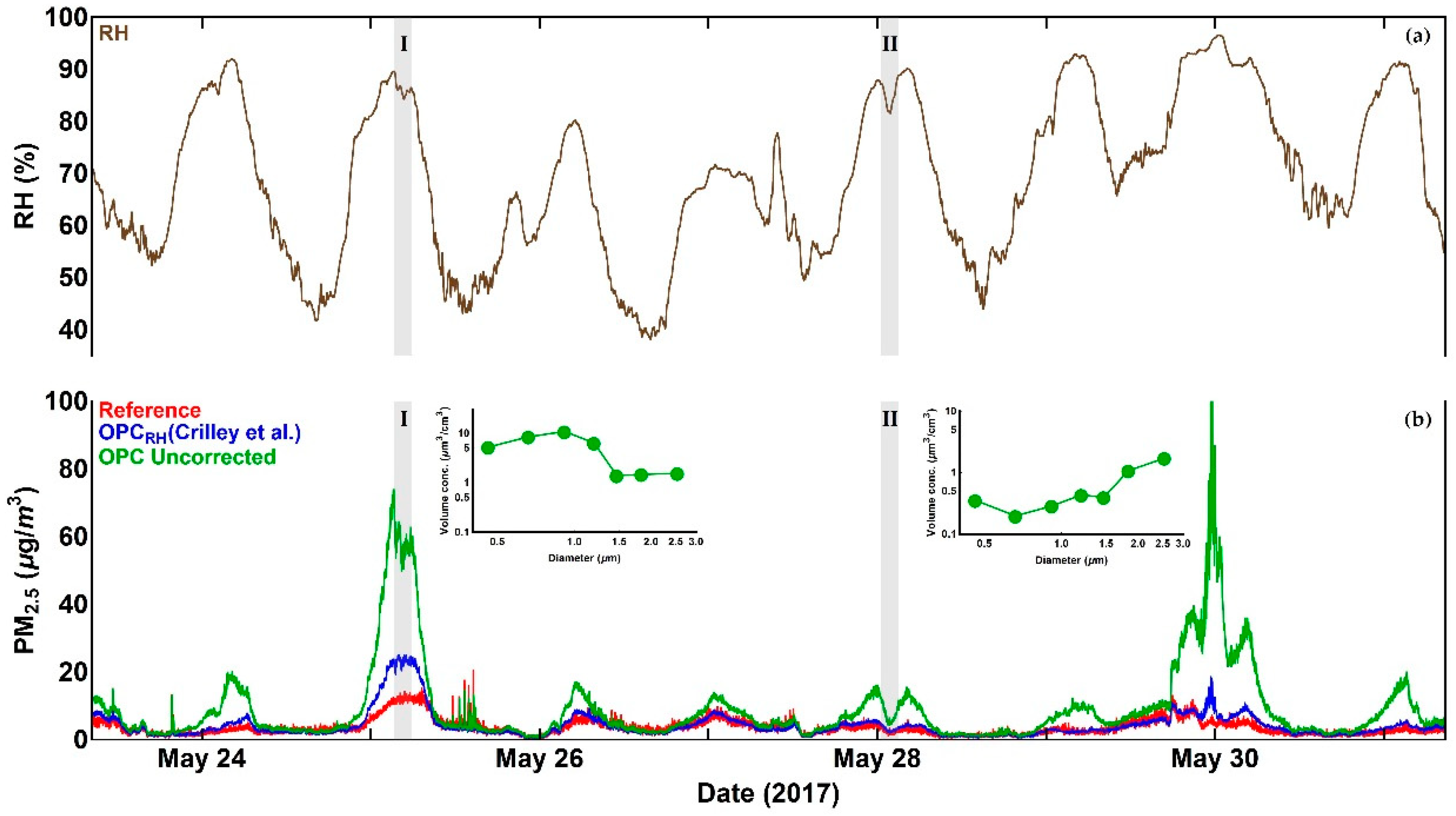
We illustrate these effects by considering a series of PM measurements from an Alphasense OPC-N2 and a Palas Fidas 200 S (certified PM reference instrument) obtained for seven days in May 2017. PM2.5 measurements for this period, before and after the application of the correction factor proposed in [16], are presented, together with reference data, in Figure 1.
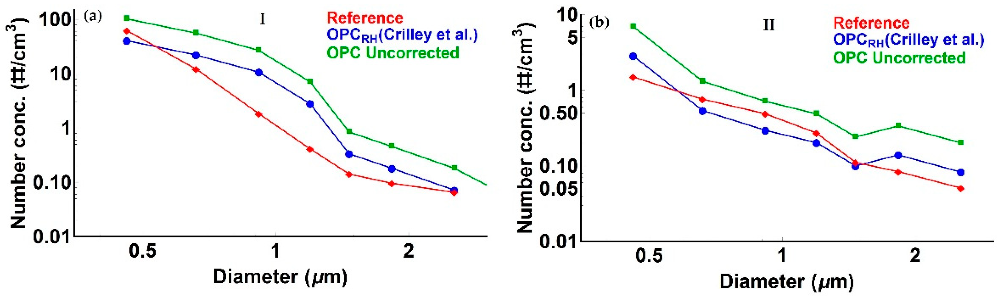
As is evident from Figure 1 and as expected, there are significant enhancements in uncorrected Alphasense OPC-N2 PM2.5 readings relative to the reference measurements associated with high RH periods, although this is not always the case (i.e., period II in Figure 1). Application of the Crilley et al. correction factor [16] improves the Alphasense OPC-N2 derived PM compared to the reference data. Nevertheless, there are multiple periods (e.g., period I in Figure 1) where significant discrepancies remain. Those periods highlight the limitation of the approach presented in [16], when the particle number concentration distribution is relatively unstructured (i.e., period II in Figure 1 and Figure 2). Under such circumstances, a shift toward smaller sizes is broadly equivalent to scaling the number concentration down by a constant factor, as illustrated in Figure 2b, where the Crilley et al. correction produces tolerable agreement with the reference dried particle distribution, so that the reference and corrected PM2.5 values broadly agree. However, when the size distribution shows significant structure (e.g., period I in Figure 1), the approach presented in [16] fails to reproduce the reference dried particle size distribution, and PM values from the corrected OPC particle size spectrum are significantly overestimated.
The aim of this paper is to introduce an improved correction algorithm where RH effects can be better described by considering the detailed particle size profile. This algorithm accounts for the RH effect on the number concentration measurements of OPCs to ensure the correct PM values are calculated and, by retaining particle physical properties ( values appropriate to specific chemical compositions), can be used to retrieve information about particles hygroscopicity and, in turn, their chemical composition.
2. Materials and Methods
2.1. Instrumentation
2.1.1. Alphasense OPC-N2
The Alphasense OPC-N2 is a low-cost portable sensor manufactured by Alphasense Ltd., in Great Notley, UK. It uses light scattering to measure size speciated particle number concentrations, which are then converted in mass concentration in the form of PM1, PM2.5 and PM10. Particles passing through the sampling volume scatter incident laser light, which is then detected by a photo detector. Based on the amount of scattered light, particle size and number concentration are both determined. Measured particle size range, dimensions, and operational settings of the instrument are presented in Table 1.
2.1.2. Palas Fidas 200 S
Palas Fidas 200 S is an EN 16450 certified static PM measurement instrument [19] manufactured by Palas GmbH in Karlsruhe, Germany. It also uses light scattering to measure particle size and particle number concentrations which are again converted into PM1, PM2.5 and PM10. However, in this case, a drying system, the Intelligent Aerosol Drying System (IADS), is used to remove water from particles before measurement. Size range, dimensions, and operational settings of Palas Fidas 200 S are presented in Table 2. Unlike the Alphasense OPC-N2, this instrument uses a white LED laser which enables the detection of particles with a diameter as small as 0.18 μm (see Table 2).
2.2. Study Area
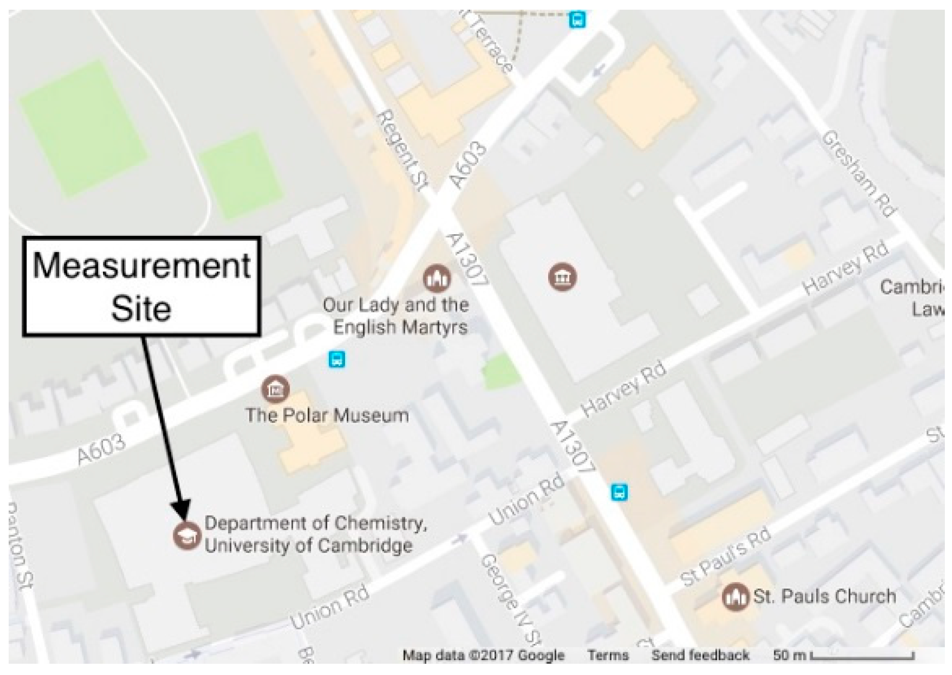
The location used for this study was the air quality and greenhouse gas monitoring station of the Centre for Atmospheric Science, University of Cambridge, UK. The measurement site is located on the roof of Chemistry Department at a height of 22 m above street level (52°11′52.4″ N, 0°07′31.9″ E). The site is close to a busy road junction in central Cambridge, as shown in Figure 3.
Alphasense OPC-N2 sensors were located in a waterproof shelter at the same height of the Palas Fidas 200 S instrument and within a distance of less than 1 m. The trials were initially performed with a single Alphasense OPC-N2 (24–31 May 2017), and then, for a more extended period (17 December 2017–16 January 2018), with two Alphasense OPC-N2 OPCs.
2.3. Data Processing
2.3.1. Data Redistribution
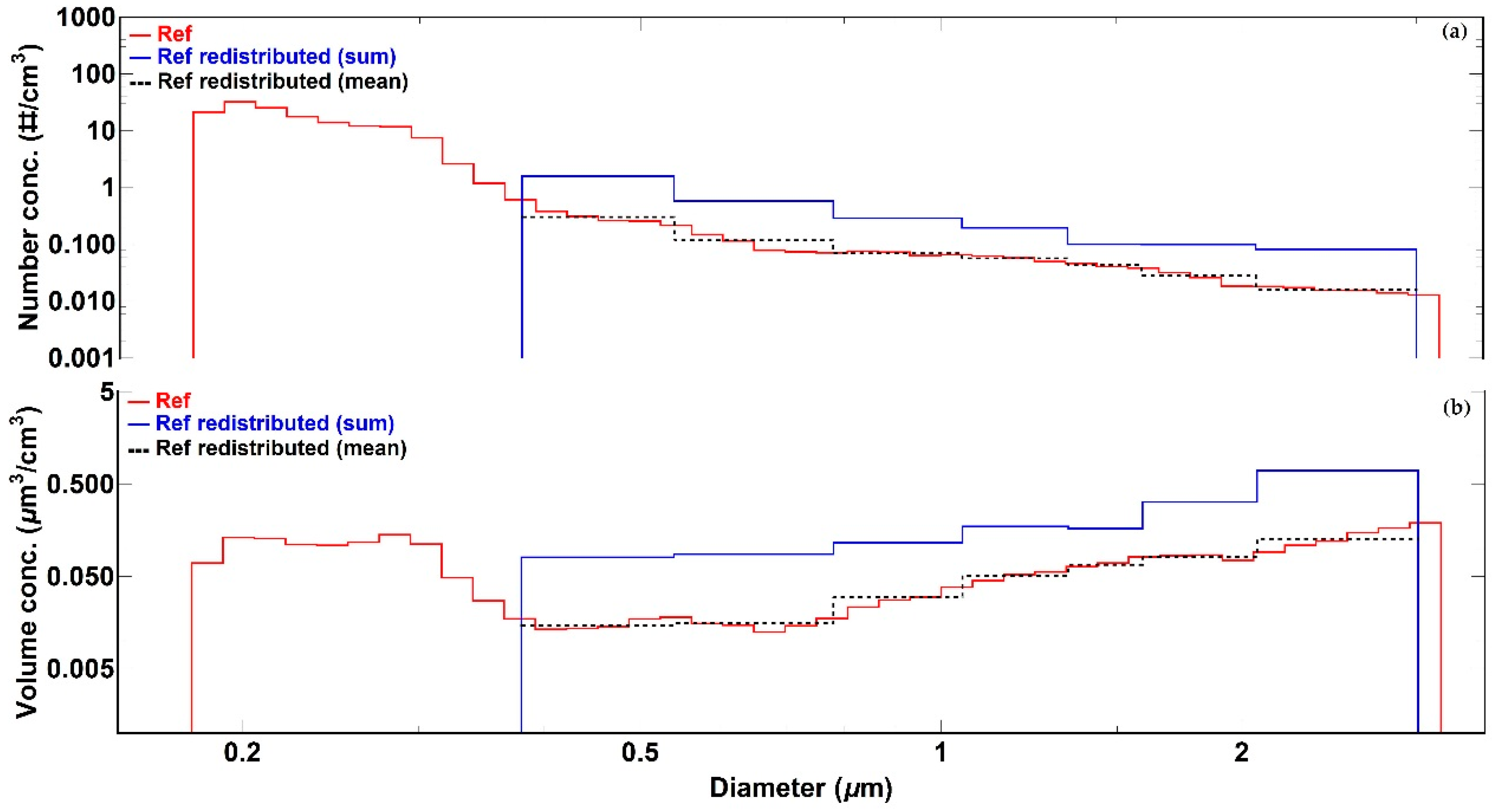
Inspection of Table 1 and Table 2 indicates that the Alphasense OPC-N2 and the reference Palas Fidas 200 S instruments have different size ranges of particle measurement with different numbers of discrete measurement bins within which individual particles are summed (16 and 64, respectively). To ensure an appropriate comparison of OPC measurements, the reference particle number concentration values were transposed on to the Alphasense OPC-N2 size range and size bins. To do so, the fraction of each reference bin in each Alphasense OPC-N2 bin range was determined. To account for the case when only the lower boundary of the reference size bin sat within an Alphasense OPC-N2 size bin, the fraction was calculated as
where is the Alphasense OPC-N2 bin, is the reference bin, and the difference is the width of the reference size bin. For the equivalent case when only the upper boundary of reference size bin sat within an Alphasense OPC-N2 size bin, the fraction was calculated as
where is the Alphasense OPC-N2 bin, is the reference bin, and the difference is the width of the reference bin. The new number concentration values for the reference data in the Alphasense OPC-N2 bins were given by the sum of all the calculated fractions within each Alphasense OPC-N2 size bins, multiplied by the associated number concentration value, as presented in Figure 4.
The advantage of using this redistribution technique is that it ensures an appropriate comparison of individual size bin data between Alphasense OPC-N2 sensors and the reference instrument. In this study, therefore, information about particle concentration in the 0.18–0.38 μm range is not used as the Alphasense OPC-N2 particle diameter detection limit is 0.38 μm (see Table 1).
2.3.2. Number Concentration to Mass Conversion
Both instruments used in this study utilise light scattering to determine particle size and particle number concentration. The conversion from particle number concentration to particle mass concentration in form of PM1, PM2.5 and PM10 is completed internally to each instrument. Particles are assumed to be spheres with uniform shape and density. In this work, the following equations were therefore used to convert particle concentration values to mass concentration:
where is the particle number concentration value for the ith bin, is the mean diameter of the ith bin, is the particle volume in the ith bin, is the particle density, and i is the bin number, spanning 1 to 16 (see Table 1). The particle density applied across all the bins from the Alphasense OPC-N2 is 1.65 g cm−3. Hence, for consistency, we used this value to calculate mass concentration values for both the OPCs and the reference instrument. PM1, expressed in μg m−3, was calculated via Equation (5) using bins 1–4. Equally, PM2.5 (μg m−3) was calculated via Equation (5) using bins 1–7. Penetration curves [20] are normally then used to convert the derived mass spectra to the appropriate PM values. However, for clarity, in the comparison of size and volume spectra for the different instruments, this step has not been applied.
2.3.3. RH Correction Algorithm
The correction algorithm presented in this study is based on the changes in particle size due to the water uptake. To quantify this effect, a hygroscopic growth factor was used [21].
where is the diameter of the dry particle and is the diameter of the particle at a given RH value. Using the -Köhler theory [17], a single parameter relationship can be used to express the RH dependence of (6) as follows [22]:
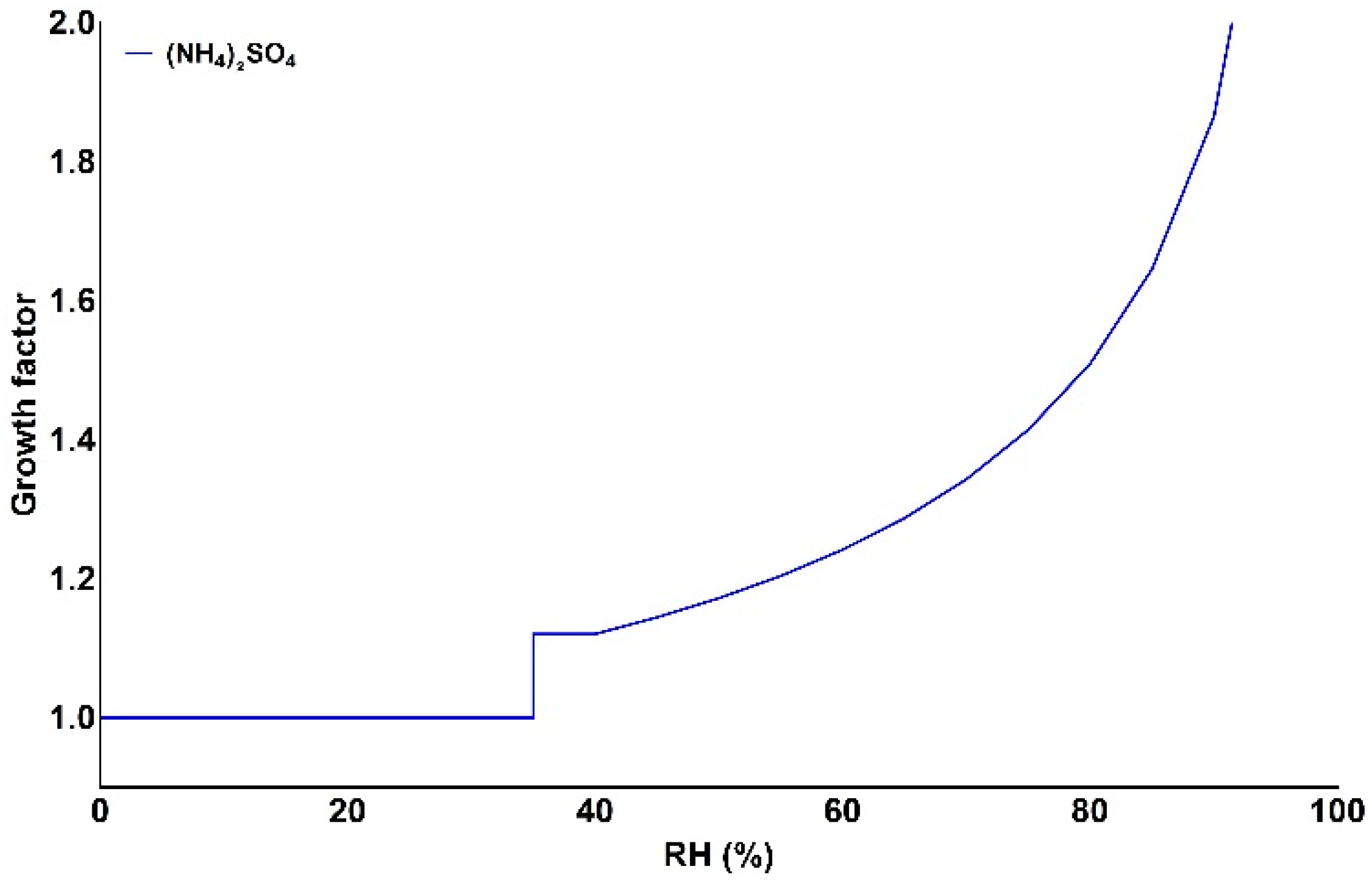
where is a parameter that describes the degree of hygroscopicity of a particle, dependent on particle composition, and RH is the relative humidity [21]. To estimate the hygroscopic growth factor, knowledge of particle composition is required. This study focuses on urban environments, where the dominant aerosol inorganic components are sulphates and nitrates [22,23]. values for ammonium sulphate and ammonium nitrate are 0.61 and 0.67 [24,25]. As reported in [26], the value for a mixture of organic and inorganic compounds in polluted environments (MIXPO), such as urban, is [26]. This mixture is a more realistic representation of the complex urban aerosol chemical composition. However, there is no information about the efflorescence point of this mixture. This implies that it is not possible to determine the RH value for which particles are no longer absorbing water. In contrast, the efflorescence point of ammonium sulphate is known to be at RH = 35% [27]. Considering the small difference in hygroscopicity of the two compounds and the information about the efflorescence point, we assumed particulate matter to be composed only of ammonium sulphate (). Under this assumption, values for 0–100% RH range, at 5% intervals, were calculated and presented in Figure 5.
From the knowledge of the hygroscopic growth factor and measurement of particle diameters at different RH values, dry diameters were calculated rearranging (6) and (7) as
The particle number concentration values, while remaining unaltered, are now associated with new, RH-corrected, size bin limits which are shifted to smaller sizes according to Equation (8). As the fundamental comparison is performed using the Alphasense bin size range, we redistribute the RH corrected particle number concentration values to the original bin size ranges using equations analogous to Equations (1) and (2) but now substituting with .
2.3.4. RH Correction Statistical Validation
To quantify the improvement of the correction method, a statistical analysis was performed, and the following parameters were calculated for PM1 and PM2.5 data: mean value of measurements, standard deviation (SD), root-mean-square error (RMSE), gradient, and coefficient of determination R2. The gradient of the scatterplot and coefficient of determination R2 were calculated assuming a linear relationship.
3. Results
3.1. Comparision of This Study with Previous Work
As outlined in the Introduction, a recent study [16] has derived a correction factor to account for the relative humidity effect on PM measurement as
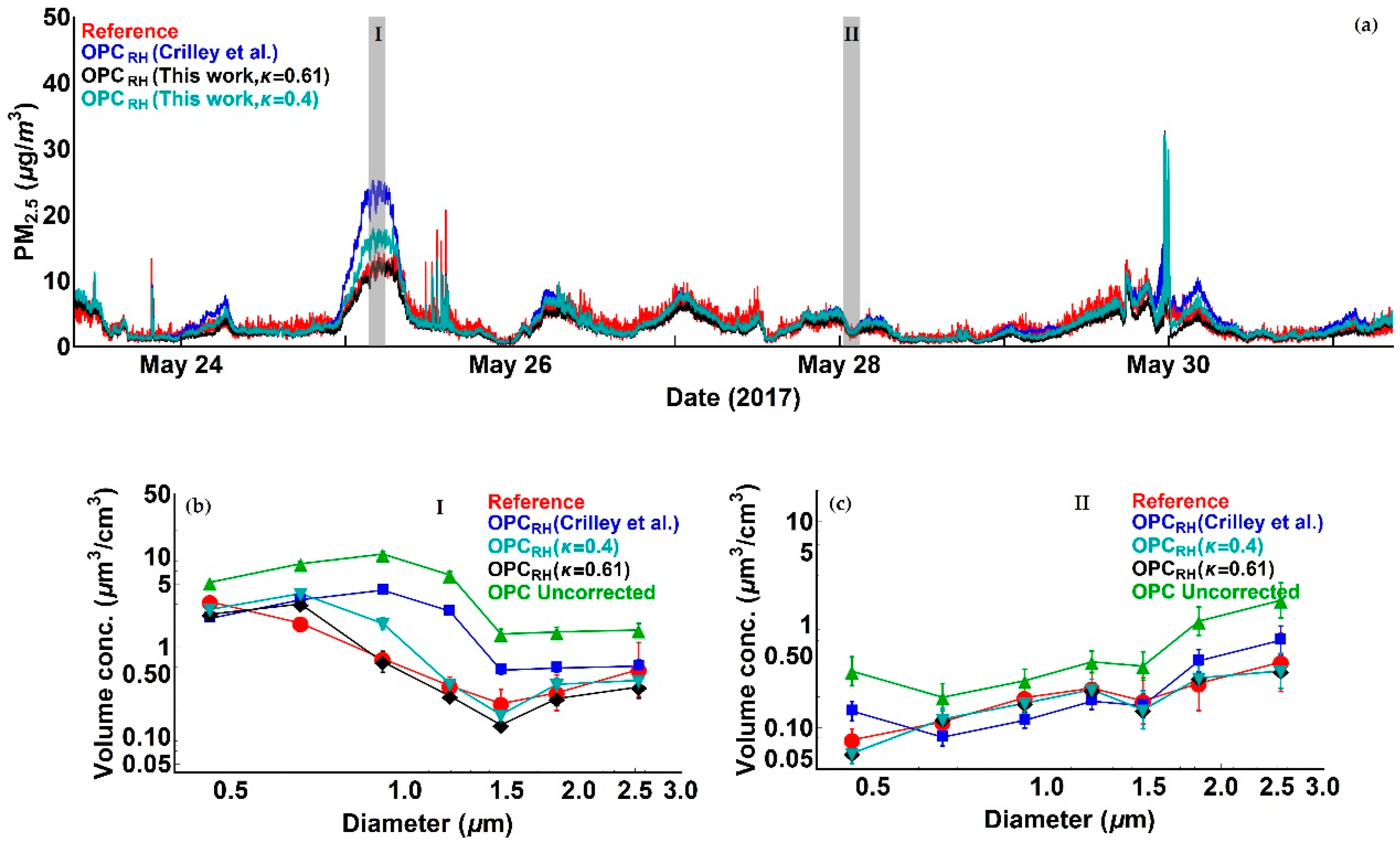
where aw is the water activity, defined as RH/100, and the statistically derived value for their data is in the 0.38–0.41 range [16]. For clarity, in this paper, we took 0.4 as the value for the correction presented in [16]. PM2.5 measurements from the Alphasense OPC-N2 between 23 May and 31 May 2017, after the application of the correction factor proposed in [16], and the correction algorithm presented in this study, in comparison with the reference data, are presented in Figure 6. To compare our correction approach to the one presented in [16], Figure 6 also presents our correction applied using two different values: 0.4, consistent with [16], and 0.61, as discussed in Section 2.3.3. As there is no information regarding the efflorescence point of the compound with = 0.4, we have assumed it to be the same as Ammonium Sulphate (RH = 35%). Also shown are particle volumes as functions of particle size for two selected periods. As previously mentioned, the size distribution for the Crilley et al. correction factor [16] has been inferred by applying a single correction factor to uncorrected OPC volume concentration data.
It is apparent from Figure 6 that, in most of cases, both correction methods significantly improve the Alphasense OPC-N2 measurements when compared to reference data. There are, however, periods where the correction factor introduced in [16] performs significantly less well (i.e., 24 May, 25 May and 30 May), while the correction algorithm proposed in this work, for both values, performs better. The discrepancy between the two correction methods can be explained by considering the changes in the particle size distributions for the different periods. The approach in [16] can be thought of as a sensitivity correction which is independent of particle size, its application leading to a uniform reduction in particle volume concentration and in turn PM. When the particle size distribution of the Alphasense OPC-N2 differs from the reference by a constant factor (Figure 6c) the single value correction approach of [16] works well. In contrast, when the particle size distribution measured by Alphasense OPC-N2 exhibits different profile from the reference (Figure 6b), this simple approach fails. The correction method presented in this work, however, shows a high level of agreement with the reference data for both periods. Moreover, when using a value of 0.61 not only we achieve better agreement in particle size distribution with reference data, but we also match the reference mass concentration values. It should be noted that both in this study and that of Crilley et al., the instruments used were the same (Alphasense OPC-N2) covering the same particle size range. As indicated in Table 1, the Alphasense OPC-N2 does not measure particles with a diameter <0.38 μm. Crilley et al. derived their kappa values by comparing their OPC measurements with TEOM measurements which capture particles below the size limit of the Alphasense OPC-N2. By doing this, their retrieved kappa value not only corrects for the RH effect but also compensates for the small particles. For these reasons, all the RH corrected data presented hereafter are calculated assuming = 0.61, unless otherwise stated.
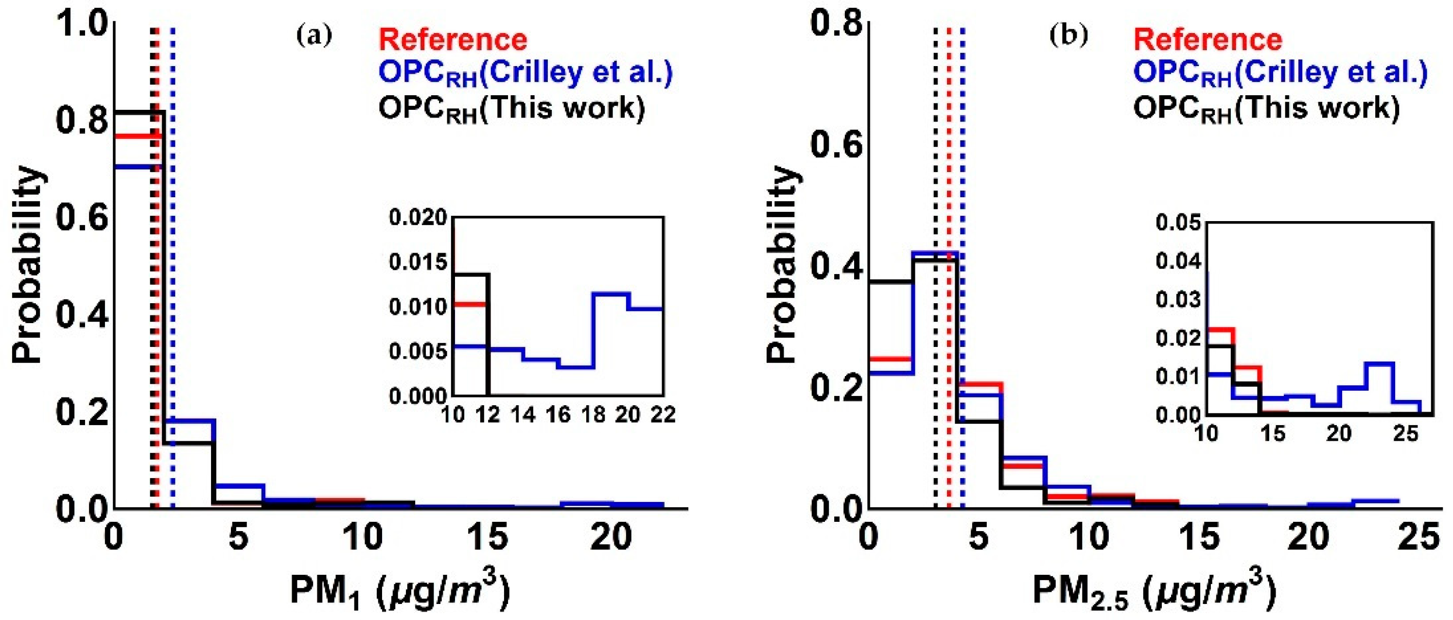
Probability distribution plots of PM1 and PM2.5 measurements for corrected Alphasense OPC-N2 and reference data are presented in Figure 7. The figure shows that while the distributions for all three sets of measurements are broadly similar, the Crilley et al. correction overestimates the number of high aerosol events for both PM1 and PM2.5. This is reflected in the averages in each case (see Table 3).
3.2. Statistical Evaluation of the RH Algorithm
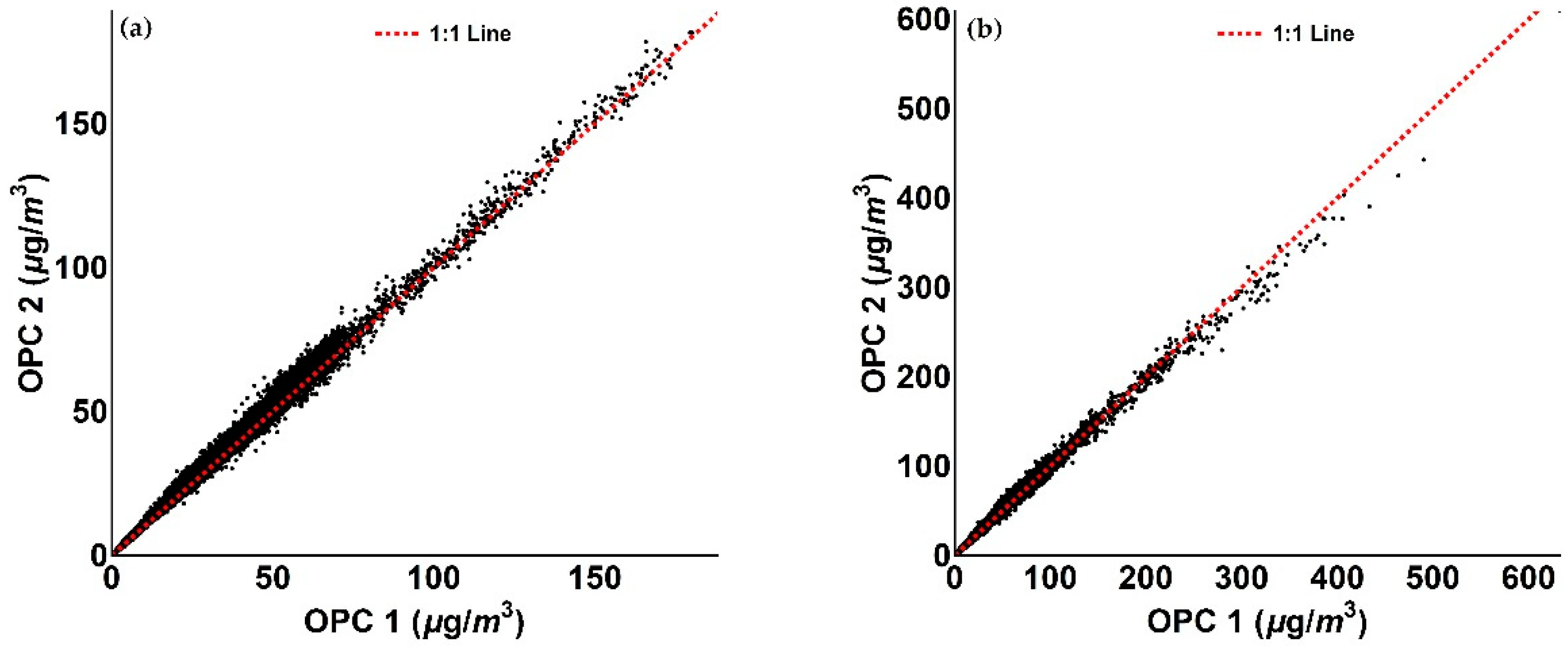
The reproducibility of the Alphasense instruments was evaluated by co-locating two OPC-N2 units in the period 17 December 2017–16 January 2018. Comparison of the two sensors are presented in Table 4 and Figure 8. Given the high level of reproducibility, the rest of this work will present measurements only from a single OPC (OPC 1).
Time series of OPC data in comparison with the reference measurements, before and after the application of the correction algorithm, are shown for PM1 and PM2.5 in Figure 9 and Figure 10 respectively.
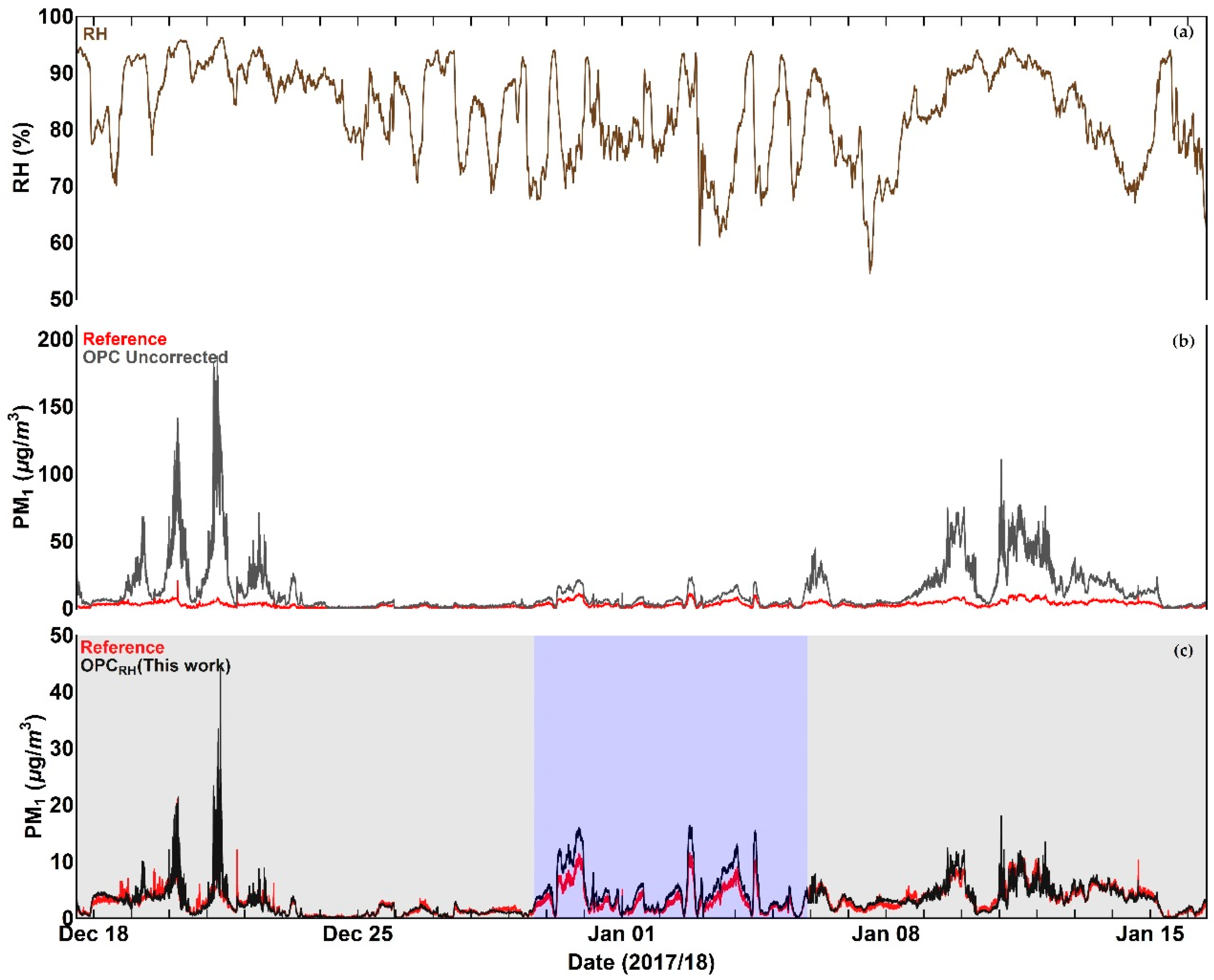
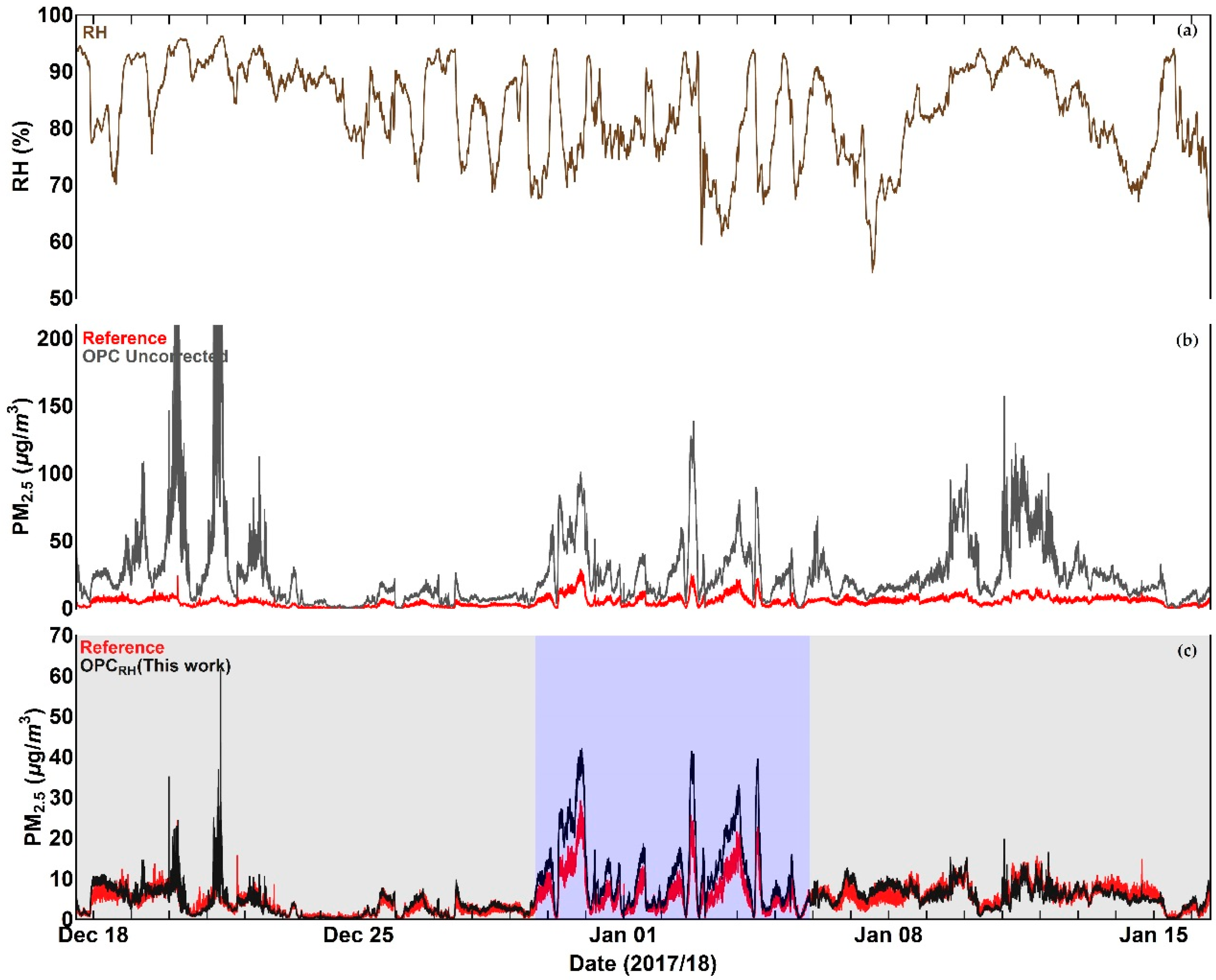
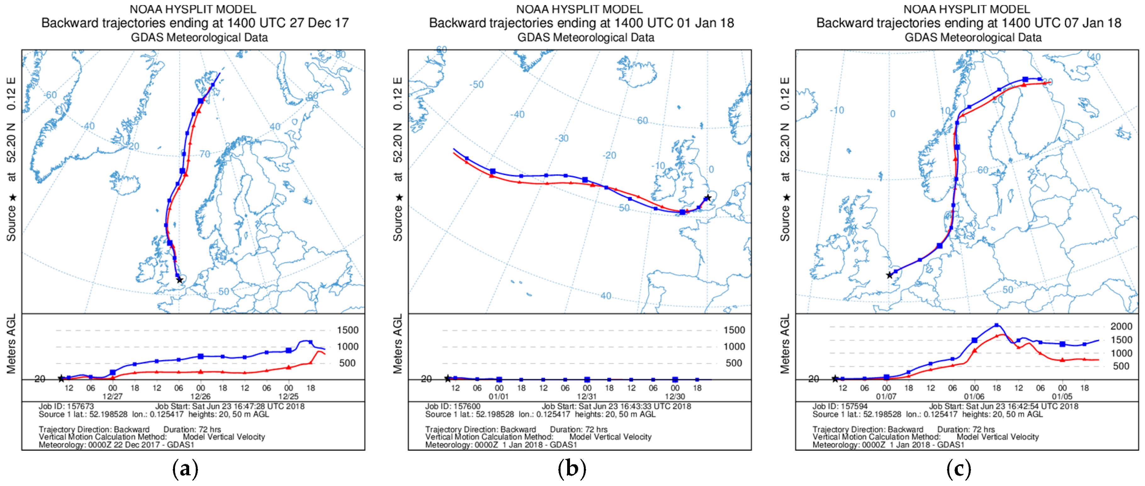
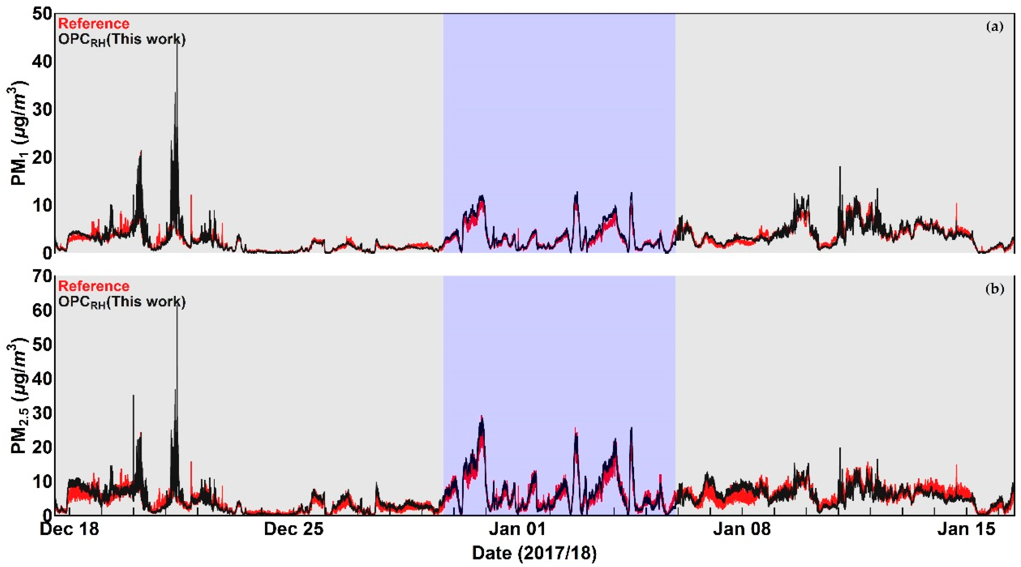
Inspection of Figure 9, Figure 10, Figure 11 and Figure 12 indicates that a substantial proportion of the RH induced peaks in the uncorrected OPC measurements are accounted for when the RH algorithm described in this work is applied, and that the level of agreement between the corrected OPCs measurements and reference data is substantially improved (see Table 5). It should be noted, however, that there remains a systematic overestimation in both PM1 and PM2.5 between 29 December 2017 and 5 January 2018 (the blue shaded area in Figure 9c and Figure 10c), suggesting that the particles are more hygroscopic (i.e., absorbing more water) during this period. To further investigate this, we ran the Ready Hysplit model developed by NOAA to determine the trajectories of air masses for the December–January period, as shown in Figure 13.
The trajectories show clear changes of air mass origin with the period in early January originating in the east Atlantic and remaining in the boundary layer throughout (Figure 13b), while the periods in Figure 13a,c originated from the Arctic mid-troposphere. It is therefore not unreasonable that there are differences in PM composition, and in fact, the early January period PM hygroscopicity is consistent with that of sodium chloride (NaCl). The sodium chloride -value is [25], and its efflorescence point is at RH = 45.5 ± 0.6% [28], i.e., more hygroscopic than ammonium sulphate. Applying the correction algorithm to the period 29 December 2017 and 5 January 2018 but changing the chemical component from ammonium sulphate to sodium chloride gives the results shown in Figure 14.
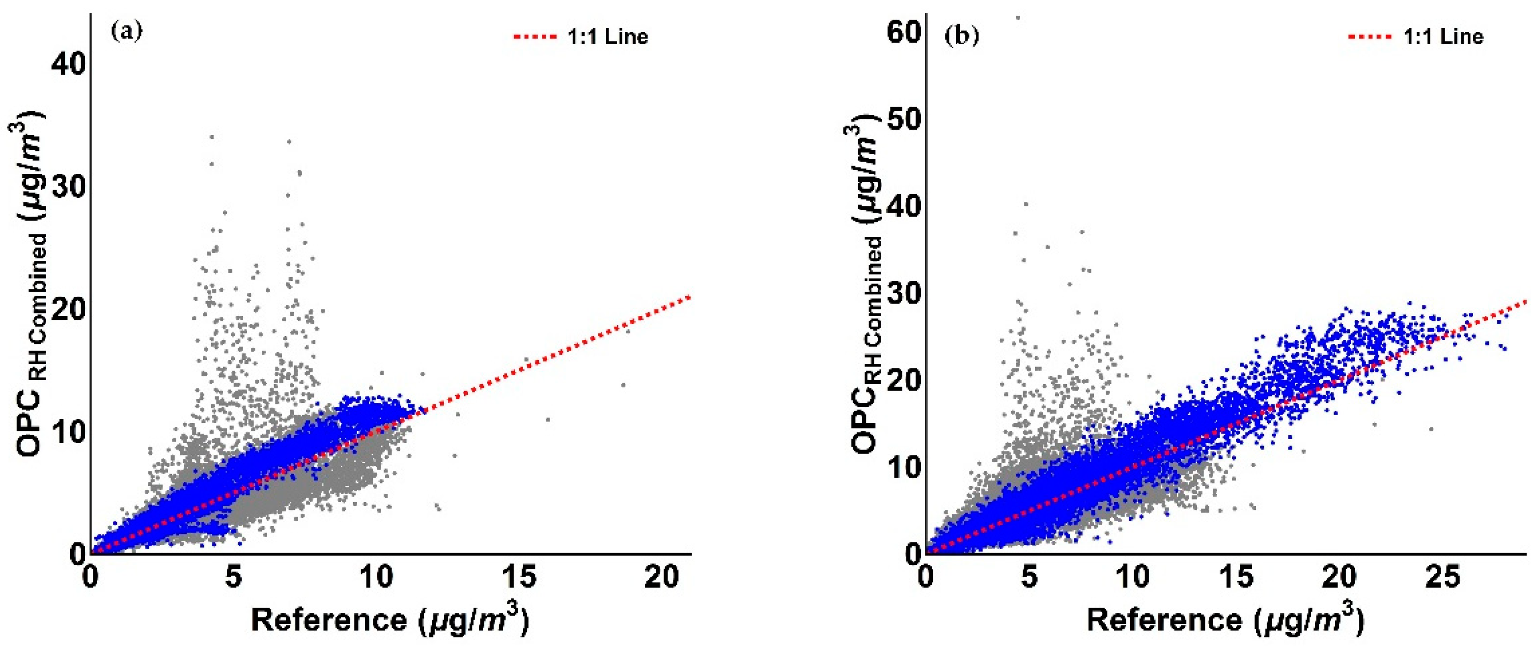
We observe from Figure 14 that by assuming NaCl as sole chemical component for this specific period (blue shaded area), the agreement of the corrected PM measurements with reference data has substantially improved. This also results in an improvement in correlation, as detailed in Figure 15.
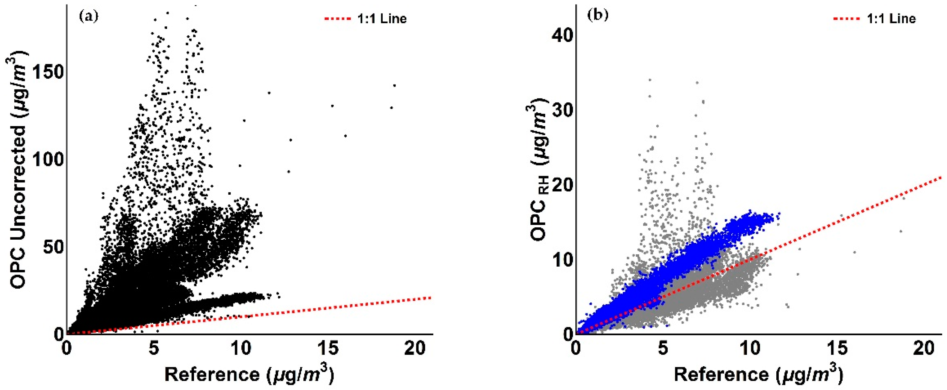
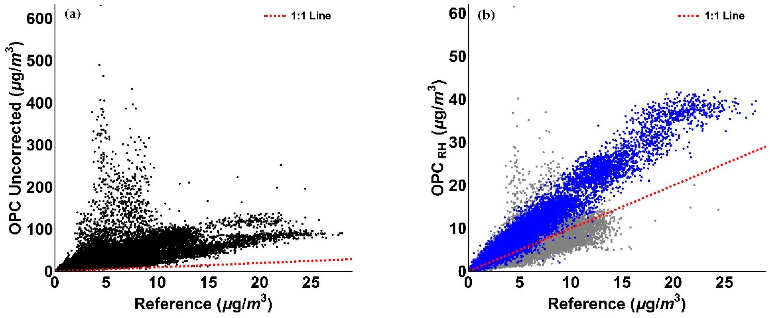
As evident from Figure 15, the measurements associated with the period where NaCl is assumed to be the sole chemical species (blue) show an improved agreement with the 1:1 line compared to assuming ammonium sulphate as the sole chemical species (cf. Figure 11b and Figure 12b).
The values reported in Table 5 confirm the improvements achieved by the correction method. When we assumed ammonium sulphate as single particle component for the 17 December 2017–16 January 2018 period, the mean value of OPC measurements was improved from a factor of 4.45 before correction to 1.15 after correction, as well as the gradient from a factor of 5.25 to a factor of 1.15 and the R2 from 0.42 to 0.73, before and after the application of the correction algorithm, respectively. When sodium chloride was assumed for the 29 December 2017–5 January 2018 period (blue shaded area in Figure 14) with ammonium sulphate elsewhere, the mean value of OPC measurements was improved from a factor of 4.45 before correction to 1.06 after correction, as well as the gradient from a factor of 5.25 to a factor of 1.05 and the R2 from 0.42 to 0.75, before and after the application of the correction algorithm, respectively. Mean values of measurements, SD, RMSE, gradient and coefficient of determination R2 values relative to PM2.5 data are presented in Table 6. As previously observed for PM1 data, values in Table 6 confirm the improvement of the RH algorithm for OPC PM2.5 measurements. Specifically, when ammonium sulphate was taken as the single particle component for the 17 December 2017–16 January 2018 period, the mean value of OPC measurements was improved from a factor of 5.10 before correction to 1.26 after correction, as well as the gradient from a factor of 4.59 to a factor of 1.43 and the R2 from 0.34 to 0.75, before and after the application of the correction algorithm, respectively. Again, when sodium chloride was assumed as sole particle component for the 29 December 2017–5 January 2018 period (blue shaded area in Figure 14) and ammonium sulphate elsewhere, the mean value of OPC measurements was improved from a factor of 5.10 before correction to 1.06 after correction, as well as the gradient from a factor of 4.59 to a factor of 1.01 and the R2 from 0.34 to 0.78, before and after the application of the correction algorithm, respectively.
4. Conclusions
Prior works have illustrated how low-cost portable sensors can be used to measure concentrations of particulate mass [11,12,29]. A recent study has focused on the effects of relative humidity on measurements [16]. However, unlike that study which proposed a correction for PM which effectively implies a uniform change in particle number at all sizes, in this study we have introduced an algorithm to correct for the changes in individual particle size due to water uptake under high RH conditions which reflects the hygroscopic properties of real world particles. The algorithm provides an adjusted particle size distribution which is not a simple scaling, and adjusted PM values. In this paper we have used measurements from a low cost OPC (Alphasense OPC-N2) and a reference OPC (Palas Fidas 200 S) over a six-week period (23 May 2017–31 May 2017 and 17 December 2017–16 January 2018). Under the assumption that urban particles consist of ammonium sulphate, we applied the correction algorithm to the Alphasense OPC-N2 measurements. The results showed that the overall level of agreement between the corrected OPC measurements and reference data was substantially improved (reduced overestimation from a factor of 5.25 to 1.15 for PM1 and from a factor of 4.59 to 1.43 for PM2.5). Nonetheless, there was a period where the corrected PM measurements still consistently overestimated the reference observations to a small degree. We show this event corresponds to a change in air mass origin consistent with a change in particle hygroscopicity. Our analysis showed that the particle hygroscopicity during this overestimation period was consistent with that of sodium chloride (NaCl). By assuming sodium chloride during the overestimation period and ammonium sulphate elsewhere, the corrected Alphasense OPC-N2 measurements improved further when compared to reference data. The results shown in this paper extend those already present in literature on the capacity of low-cost sensors to give reliable ambient PM readings when an appropriate correction is applied. While this work was performed using the instrument characteristics of an Alphasense OPC-N2, this algorithm is independent of sensor type and can be readily adapted to other size speciated particle counters and different environments. Finally, we note that the correction algorithm presented in this work not only is flexible to changes in particle chemical composition but also leads to the possibility of particle chemical speciation using low-cost sensors.
Author Contributions
Conceptualization, A.D.A., O.A.M.P. and R.L.J.; Data curation, A.D.A., O.A.M.P., B.O., J.S. and R.L.J.; Formal analysis, A.D.A., O.A.M.P. and R.L.J.; Methodology, A.D.A., O.A.M.P., B.O. and R.L.J.; Resources, J.S. and R.L.J.; Software, A.D.A., O.A.M.P. and R.L.J.; Supervision, R.L.J.; Validation, R.L.J.; Visualization, A.D.A., O.A.M.P. and B.O.; Writing—original draft, A.D.A.; Writing—review & editing, A.D.A. and R.L.J.
Funding
This research received no external funding.
Acknowledgments
Andrea Di Antonio acknowledges the support from Alphasense Ltd. for his PhD project.
Conflicts of Interest
The authors declare no conflict of interest.
References
- Laden, F.; Neas, L.M.; Dockery, D.W.; Schwartz, J. Association of fine particulate matter from different sources with daily mortality in six U.S. cities. Environ. Health Perspect. 2000, 108, 941–947. [Google Scholar] [CrossRef] [PubMed]
- Laden, F.; Schwartz, J.; Speizer, F.E.; Dockery, D.W. Reduction in Fine Particulate Air Pollution and Mortality. Am. J. Respir. Crit. Care Med. 2006, 173, 667–672. [Google Scholar] [CrossRef] [PubMed] [Green Version]
- Dockery, D.W.; Pope, C.A.; Xu, X.; Spengler, J.D.; Ware, J.H.; Fay, M.E.; Ferris, B.G.; Speizer, F.E. An Association between Air Pollution and Mortality in Six U.S. Cities. N. Engl. J. Med. 1993, 329, 1753–1759. [Google Scholar] [CrossRef] [PubMed]
- Pope, C.A.; Dockery, D.W. Health Effects of Fine Particulate Air Pollution: Lines that Connect. J. Air Waste Manag. Assoc. 2006, 56, 709–742. [Google Scholar] [CrossRef] [PubMed] [Green Version]
- World Health Organization (WHO). Air Quality Guidelines for Particulate Matter, Ozone, Nitrogen Dioxide and Sulfur Dioxide; WHO: Geneva, Switzerland, 2005. [Google Scholar]
- The European Parliament and of the Council of the European Union. Directive 2008/50/EC of the European Parliament and of the council of 21 May 2008 on ambient air quality and cleaner air for Europe. Off. J. Eur. Union 2008, 11, L1–L44. [Google Scholar]
- Mar, T.F.; Larson, T.V.; Stier, R.A.; Claiborn, C.; Koenig, J.Q. An Analysis of the Association between Respiratory Symptoms in Subjects with Asthma and Daily Air Pollution in Spokane, Washington. Inhal. Toxicol. 2004, 16, 809–815. [Google Scholar] [CrossRef] [PubMed]
- Lighty, J.S.; Veranth, J.M.; Sarofim, A.F. Combustion Aerosols: Factors Governing Their Size and Composition and Implications to Human Health. J. Air Waste Manag. Assoc. 2000, 50, 1565–1618. [Google Scholar] [CrossRef] [PubMed] [Green Version]
- Jerrett, M.; Burnett, R.T.; Ma, R.; Pope, C.A.; Krewski, D.; Newbold, K.B.; Thurston, G.; Shi, Y.; Finkelstein, N.; Calle, E.E.; et al. Spatial Analysis of Air Pollution and Mortality in Los Angeles. Epidemiology 2005, 16, 727–736. [Google Scholar] [CrossRef] [PubMed] [Green Version]
- Jerrett, M.; Finkelstein, M. Geographies of Risk in Studies Linking Chronic Air Pollution Exposure to Health Outcomes. J. Toxicol. Environ. Heal. Part A 2005, 68, 1207–1242. [Google Scholar] [CrossRef] [PubMed]
- Jovašević-Stojanović, M.; Bartonova, A.; Topalović, D.; Lazović, I.; Pokrić, B.; Ristovski, Z. On the use of small and cheaper sensors and devices for indicative citizen-based monitoring of respirable particulate matter. Environ. Pollut. 2015, 206, 696–704. [Google Scholar] [CrossRef] [PubMed]
- Gao, M.; Cao, J.; Seto, E. A distributed network of low-cost continuous reading sensors to measure spatiotemporal variations of PM2.5 in Xi’an, China. Environ. Pollut. 2015, 199, 56–65. [Google Scholar] [CrossRef] [PubMed]
- Sousan, S.; Koehler, K.; Hallett, L.; Peters, T.M. Evaluation of the Alphasense Optical Particle Counter (OPC-N2) and the Grimm Portable Aerosol Spectrometer (PAS-1.108). Aerosol Sci. Technol. 2016, 50, 1352–1365. [Google Scholar] [CrossRef] [PubMed]
- Steinle, S.; Reis, S.; Sabel, C.E.; Semple, S.; Twigg, M.M.; Braban, C.F.; Leeson, S.R.; Heal, M.R.; Harrison, D.; Lin, C.; et al. Personal exposure monitoring of PM2.5 in indoor and outdoor microenvironments. Sci. Total Environ. 2015, 508, 383–394. [Google Scholar] [CrossRef] [PubMed]
- Lundgren, D.A.; Cooper, D.W. Effect of Humidity on Light-Scattering Methods of Measuring Particle Concentration. J. Air Pollut. Control Assoc. 1969, 19, 243–247. [Google Scholar] [CrossRef]
- Crilley, L.R.; Shaw, M.; Pound, R.; Kramer, L.J.; Price, R.; Young, S.; Lewis, A.C.; Pope, F.D. Evaluation of a low-cost optical particle counter (Alphasense OPC-N2) for ambient air monitoring. Atmos. Meas. Tech. 2018, 11, 709–720. [Google Scholar] [CrossRef] [Green Version]
- Kohler, H. The Nucleus in and the Growth of Hygroscopic Droplets. Trans. Faraday Soc. 1936, 32, 1152–1161. [Google Scholar] [CrossRef]
- Alphasense Ltd. OPC-N2 Technical Specification. Available online: http://www.alphasense.com/WEB1213/wp-content/uploads/2017/05/OPC-N2.pdf (accessed on 18 July 2017).
- Fidas® 200 S Technical Specification. Available online: https://www.palas.de/en/product/fidas200s (accessed on 18 July 2017).
- European Committee for Standardization. Workplace Atmospheres-Size Fraction Definitions for Measurement of Airborne Particles; CEN: London, UK, 1993. [Google Scholar]
- Zieger, P.; Fierz-Schmidhauser, R.; Weingartner, E.; Baltensperger, U. Effects of relative humidity on aerosol light scattering: Results from different European sites. Atmos. Chem. Phys. 2013, 13, 10609–10631. [Google Scholar] [CrossRef]
- Petters, M.D.; Kreidenweis, S.M. A single parameter representation of hygroscopic growth and cloud condensation nucleus activity. Atmos. Chem. Phys. 2007, 7, 1961–1971. [Google Scholar] [CrossRef] [Green Version]
- Allan, J.D.; Alfarra, M.R.; Bower, K.N.; Williams, P.I.; Gallagher, M.W.; Jimenez, J.L.; Mcdonald, A.G.; Nemitz, E.; Canagaratna, M.R.; Jayne, J.T.; et al. Quantitative sampling using an Aerodyne aerosol mass spectrometer 2. Measurements of fine particulate chemical composition in two U.K. cities. J. Geophys. Res. 2003, 108, 107–118. [Google Scholar]
- John, W.; Wall, S.M.; Ondo, J.L.; Winklmayr, W. Modes in the size distributions of atmospheric inorganic aerosol. Atmos. Environ. Part A. Gen. Top. 1990, 24, 2349–2359. [Google Scholar] [CrossRef]
- Clegg, S.L.; Brimblecombe, P.; Wexler, A.S. Thermodynamic Model of the System H+−NH4+−SO42−−NO3−−H2O at Tropospheric Temperatures. J. Phys. Chem. A 1998, 102, 2137–2154. [Google Scholar] [CrossRef]
- Svenningsson, B.; Rissler, J.; Swietlicki, E.; Mircea, M.; Bilde, M.; Facchini, M.C.; Decesari, S.; Fuzzi, S.; Zhou, J.; Mønster, J.; et al. Hygroscopic growth and critical supersaturations for mixed aerosol particles of inorganic and organic compounds of atmospheric relevance. Atmos. Chem. Phys. 2006, 6, 1937–1952. [Google Scholar] [CrossRef] [Green Version]
- Liu, Y.; Yang, Z.; Desyaterik, Y.; Gassman, P.L.; Wang, H.; Laskin, A. Hygroscopic Behavior of Substrate-Deposited Particles Studied by Micro-FT-IR Spectroscopy and Complementary Methods of Particle Analysis. Anal. Chem. 2008, 80, 7179. [Google Scholar] [CrossRef]
- Richardson, C.B.; Snyder, T.D. A Study of Heterogeneous Nucleation in Aqueous Solutions. Langmuir 1994, 10, 2462–2465. [Google Scholar] [CrossRef]
- Northcross, A.L.; Edwards, R.J.; Johnson, M.A.; Wang, Z.M.; Zhu, K.; Allen, T.; Smith, K.R. A low-cost particle counter as a realtime fine-particle mass monitor. Environ. Sci. Process. Impacts 2013, 15, 433–439. [Google Scholar] [CrossRef] [PubMed]
Figure 1.
Time series of Alphasense OPC-N2 PM2.5 measurements compared with reference data: (a) Time series of relative humidity; (b) Time series of Alphasense OPC-N2 PM2.5 measurements, before and after the application of the Crilley et al. correction factor, in comparison with reference data. The two inserts show volume distribution profiles measured by the uncorrected OPC-N2 for periods I and II. The overall measurement period consists of seven consecutive days data between 23 May and 31 May 2017. See text for discussion. (PM: particulate matter).

Figure 2.
Particle size distributions for (a) period I in Figure 1 and (b) period II in Figure 1. Uncorrected Alphasense OPC-N2 particle size distributions are shown in green. Particle size distributions after application of the Crilley et al. correction factor (assumed to be constant across the size spectrum) are shown in blue, and reference data in red. See text for discussion.

Figure 3.
Map showing the location of measurement site in Cambridge, UK. Courtesy of Google Maps.

Figure 4.
Illustration of Palas Fidas 200 S measurements redistributed into the Alphasense OPC-N2 size bins for all bins contributing to PM2.5 for (a) number concentration data and (b) volume concentration data. The black dashed lines represent the average Palas Fidas 200 S measurements in each Alphasense size bin.

Figure 5.
Growth factor curve as function of relative humidity (RH) for ammonium sulphate. The discontinuity represents the efflorescence point of the compound [27].
Figure 5.
Growth factor curve as function of relative humidity (RH) for ammonium sulphate. The discontinuity represents the efflorescence point of the compound [27].

Figure 6.
Figures illustrating Alphasense OPC-N2 measurements in comparison with reference data. (a) Time series of Alphasense OPC-N2 PM2.5 measurements after the application of the correction factor [16] and the correction algorithm (this work) assuming a value of 0.4 (Cyan) and 0.61 (Black) in comparison with reference data; (b) Size distribution of Alphasense OPC-N2 volume concentration data for all size bins contributing to PM2.5 before and after the application of the correction factor [16] and the correction algorithm (this work) assuming a value of 0.4 (Cyan) and 0.61 (Black) in comparison with reference data for period I (25 May 03:18:00 UTC–25 May 05:48:00 UTC); (c) as (b) except for period II (28 May 00:31:00 UTC–28 May 03:01:00 UTC).

Figure 7.
Probability distribution plot of Alphasense OPC-N2 measurement, after the application of the correction factor [16] and the correction algorithm (this work), in comparison with reference data for (a) PM1 and (b) PM2.5. The dashed lines represent the mean of PM values in each case. The inserts figures show PM probabilities at higher values on expanded scales (see text).

Figure 8.
Figures illustrating the reproducibility of the two Alphasense OPC-N2. (a) Scatter plot of OPC 1 and OPC 2 PM1 measurement relative to the period between 17 December 2017 and 16 January 2018; (b) OPC 1 and OPC 2 PM2.5 measurement scatter plot of OPC 1 and OPC 2 PM1 measurement relative to the period between 17 December 2017 and 16 January 2018.

Figure 9.
Time series plots of (a) Relative Humidity, (b) OPC PM1 measurement in comparison with reference data before the application of the correction algorithm, and (c) OPC PM1 measurement in comparison with reference after the application of the correction algorithm. The blue shaded area denotes a period during which the corrected PM values show a systematic overestimation compared to with reference data. More details are given in the text.

Figure 10.
Time series plots of (a) Relative Humidity, (b) OPC PM2.5 measurement in comparison with reference data before the application of the correction algorithm, and (c) OPC PM2.5 measurement in comparison with reference after the application of the correction algorithm. The blue shaded area denotes a period during which the corrected PM values show a systematic overestimation compared to with reference data. More details are given in the text.

Figure 11.
Figures illustrating the comparison of OPC measurements with reference data for PM1 values. (a) Scatter plot of reference and uncorrected OPC PM1 measurements relative to the period between 17 December 2017 and 16 January 2018; (b) Scatter plot of reference and OPC RH-corrected PM1 measurements relative to the period between 17 December 2017 and 16 January 2018. The colour scheme reflects the blue and grey shaded areas in Figure 9c.

Figure 12.
Figures illustrating the comparison of OPC measurements with reference data for PM2.5 values. (a) Scatter plot of reference and uncorrected OPC PM2.5 measurements relative to the period between 17 December 2017 and 16 January 2018; (b) Scatter plot of reference and OPC RH-corrected PM1 measurements relative to the period between 17 December 2017 and 16 January 2018. The colour scheme reflects the blue and grey shaded areas in Figure 10c.

Figure 13.
Ready Hysplit air mass trajectories plots ending in Cambridge (UK). (a) 27 December 2017; (b) 1 January 2018; (c) 7 January 2018. The blue and red lines correspond to trajectories at 20 m and 50 m above ground level, respectively.
Figure 13.
Ready Hysplit air mass trajectories plots ending in Cambridge (UK). (a) 27 December 2017; (b) 1 January 2018; (c) 7 January 2018. The blue and red lines correspond to trajectories at 20 m and 50 m above ground level, respectively.

Figure 14.
Time series plots of OPC PM measurements in comparison with reference data after the application of the correction algorithm assuming Ammonium Sulphate (grey shaded area) and Sodium Chloride (blue shaded area) as unique particle chemical species for: (a) PM1; (b) PM2.5.
Figure 14.
Time series plots of OPC PM measurements in comparison with reference data after the application of the correction algorithm assuming Ammonium Sulphate (grey shaded area) and Sodium Chloride (blue shaded area) as unique particle chemical species for: (a) PM1; (b) PM2.5.

Figure 15.
Figures illustrating the comparison of RH corrected PM measurements assuming Ammonium Sulphate (grey points) and Sodium Chloride (blue points) as unique chemical species for PM for the periods discussed above. (a) PM1; (b) PM2.5.
Figure 15.
Figures illustrating the comparison of RH corrected PM measurements assuming Ammonium Sulphate (grey points) and Sodium Chloride (blue points) as unique chemical species for PM for the periods discussed above. (a) PM1; (b) PM2.5.


Table 1.
Summary of Alphasense OPC-N2 operational settings [18].
Table 1.
Summary of Alphasense OPC-N2 operational settings [18].
| Alphasense OPC-N2 | |
|---|---|
| Sampling time (s) | 1.4 |
| Size range (µm) | 0.38–17.0 |
| Number of size bins | 16 |
| Flow rate (L/min) | 1.2 |
| Data storage (GB) | 16 |
| Weight (Kg) | 0.105 |
| Dimensions H·W·D (mm) | 63.5 × 75 × 60 |
| Temperature range (°C) | −10 to +50 |
Table 2.
Summary of Palas Fidas 200 operational settings [19].
Table 2.
Summary of Palas Fidas 200 operational settings [19].
| Palas Fidas 200 S | |
|---|---|
| Sampling time (s) | 60 (average) |
| Size range (µm) | 0.18–18.0 |
| Number of size bins | 64 |
| Flow rate (L/min) | 4.8 |
| Data storage (GB) | 4 |
| Weight (Kg) | 60 |
| Dimensions H·W·D (mm) | 1810 × 600 × 400 |
| Temperature range (°C) | −20 to +50 |
Table 3.
Average PM values for the corrected OPC and reference measurements in Figure 6.
Table 3.
Average PM values for the corrected OPC and reference measurements in Figure 6.
| Reference | Crilley et al. | This Work | |
|---|---|---|---|
| PM1 (μg/m3) | 1.74 | 2.36 | 1.55 |
| PM2.5 (μg/m3) | 3.64 | 4.25 | 3.03 |
Table 4.
Correlation values for Alphasense OPC-N2 sensors used during this study.
| OPC | PM1 | PM2.5 | ||
|---|---|---|---|---|
| Gradient | R2 | Gradient | R2 | |
| 1 | 1.00 | 1.00 | 1.00 | 1.00 |
| 2 | 1.03 | 0.99 | 0.99 | 0.99 |
Table 5.
Statistical parameters for PM1 measurement of reference, uncorrected OPC, and OPC after the application of the RH algorithm.
Table 5.
Statistical parameters for PM1 measurement of reference, uncorrected OPC, and OPC after the application of the RH algorithm.
| PM1 | Reference | OPC (Uncorrected) | OPC (RH Corrected) | OPC (RH Combined) |
|---|---|---|---|---|
| Mean (µg/m3) | 3.02 | 13.45 | 3.46 | 3.20 |
| SD (µg/m3) | 2.25 | 18.24 | 3.03 | 2.72 |
| RMSE (µg/m3) | N.A. | 19.84 | 1.66 | 1.37 |
| Gradient | 1.00 | 5.25 | 1.15 | 1.05 |
| R2 | 1.00 | 0.42 | 0.73 | 0.75 |
| Number of points | 43,000 | 43,000 | 43,000 | 43,000 |
Table 6.
Statistical parameters for PM2.5 measurement of reference, uncorrected OPC, and OPC after the application of the RH algorithm.
Table 6.
Statistical parameters for PM2.5 measurement of reference, uncorrected OPC, and OPC after the application of the RH algorithm.
| PM2.5 | Reference | OPC (Uncorrected) | OPC (RH Corrected) | OPC (RH Combined) |
|---|---|---|---|---|
| Mean (µg/m3) | 5.12 | 26.10 | 6.47 | 5.44 |
| SD (µg/m3) | 3.69 | 28.85 | 6.07 | 4.21 |
| RMSE (µg/m3) | N.A. | 35.78 | 5.91 | 3.74 |
| Gradient | 1.00 | 4.59 | 1.43 | 1.01 |
| R2 | 1.00 | 0.34 | 0.75 | 0.78 |
| Number of points | 43,000 | 43,000 | 43,000 | 43,000 |
© 2018 by the authors. Licensee MDPI, Basel, Switzerland. This article is an open access article distributed under the terms and conditions of the Creative Commons Attribution (CC BY) license (http://creativecommons.org/licenses/by/4.0/).
Share and Cite
MDPI and ACS Style
Di Antonio, A.; Popoola, O.A.M.; Ouyang, B.; Saffell, J.; Jones, R.L. Developing a Relative Humidity Correction for Low-Cost Sensors Measuring Ambient Particulate Matter. Sensors 2018, 18, 2790. https://doi.org/10.3390/s18092790
AMA Style
Di Antonio A, Popoola OAM, Ouyang B, Saffell J, Jones RL. Developing a Relative Humidity Correction for Low-Cost Sensors Measuring Ambient Particulate Matter. Sensors. 2018; 18(9):2790. https://doi.org/10.3390/s18092790
Chicago/Turabian StyleDi Antonio, Andrea, Olalekan A. M. Popoola, Bin Ouyang, John Saffell, and Roderic L. Jones. 2018. "Developing a Relative Humidity Correction for Low-Cost Sensors Measuring Ambient Particulate Matter" Sensors 18, no. 9: 2790. https://doi.org/10.3390/s18092790
Note that from the first issue of 2016, this journal uses article numbers instead of page numbers. See further details here.