Face Recognition Systems: A Survey

1
AI-ED Department, Yncrea Ouest, 20 rue du Cuirassé de Bretagne, 29200 Brest, France
2
Electronic and Micro-electronic Laboratory, Faculty of Sciences of Monastir, University of Monastir, Monastir 5000, Tunisia
3
College of Computer Science, King Khalid University, Abha 61421, Saudi Arabia
*
Author to whom correspondence should be addressed.
Sensors 2020, 20(2), 342; https://doi.org/10.3390/s20020342
Submission received: 15 October 2019
/
Revised: 12 December 2019
/
Accepted: 15 December 2019
/
Published: 7 January 2020
(This article belongs to the Special Issue Biometric Systems)
Abstract
:Over the past few decades, interest in theories and algorithms for face recognition has been growing rapidly. Video surveillance, criminal identification, building access control, and unmanned and autonomous vehicles are just a few examples of concrete applications that are gaining attraction among industries. Various techniques are being developed including local, holistic, and hybrid approaches, which provide a face image description using only a few face image features or the whole facial features. The main contribution of this survey is to review some well-known techniques for each approach and to give the taxonomy of their categories. In the paper, a detailed comparison between these techniques is exposed by listing the advantages and the disadvantages of their schemes in terms of robustness, accuracy, complexity, and discrimination. One interesting feature mentioned in the paper is about the database used for face recognition. An overview of the most commonly used databases, including those of supervised and unsupervised learning, is given. Numerical results of the most interesting techniques are given along with the context of experiments and challenges handled by these techniques. Finally, a solid discussion is given in the paper about future directions in terms of techniques to be used for face recognition.
1. Introduction
The objective of developing biometric applications, such as facial recognition, has recently become important in smart cities. In addition, many scientists and engineers around the world have focused on establishing increasingly robust and accurate algorithms and methods for these types of systems and their application in everyday life. All types of security systems must protect all personal data. The most commonly used type for recognition is the password. However, through the development of information technologies and security algorithms, many systems are beginning to use many biometric factors for recognition task [1,2,3,4]. These biometric factors make it possible to identify people’s identity by their physiological or behavioral characteristics. They also provide several advantages, for example, the presence of a person in front of the sensor is sufficient, and there is no more need to remember several passwords or confidential codes anymore. In this context, many recognition systems based on different biometric factors such as iris, fingerprints [5], voice [6], and face have been deployed in recent years.
Systems that identify people based on their biological characteristics are very attractive because they are easy to use. The human face is composed of different structures and characteristics. For this reason, in recent years, it has become one of the most widely used biometric authentication systems, given its potential in many applications and fields (surveillance, home security, border control, and so on) [7,8,9]. Facial recognition system as an ID (identity) is already being offered to consumers outside of phones, including at airport check-ins, sports stadiums, and concerts. In addition, this system does not require the intervention of people to operate, which makes it possible to identify people only from images obtained from the camera. In addition, many biometric systems that are developed using different types of search provide good identification accuracy. However, it would be interesting to develop new biometric systems for face recognition in order to reach real-time constraints.
Owing to the huge volume of data generated and rapid advancement in artificial intelligence techniques, traditional computing models have become inadequate to process data, especially for complex applications like those related to feature extraction. Graphics processing units (GPUs) [4], central processing unit (CPU) [3], and programmable gate arrays (FPGAs) [10] are required to efficiently perform complex computing tasks. GPUs have computing cores that are several orders of magnitude larger than traditional CPU and allow greater capacity to perform parallel computing. Unlike GPUs, the FPGAs have a flexible hardware configuration and offer better performance than GPUs in terms of energy efficiency. However, FPGAs present a major drawback related to the programming time, which is higher than that of CPU and GPU.
There are many computer vision approaches proposed to address face detection or recognition tasks with high robustness and discrimination, such as local, subspace, and hybrid approaches [10,11,12,13,14,15,16]. However, several issues still need to be addressed owing to various challenges, such as head orientation, lighting conditions, and facial expression. The most interesting techniques are developed to face all these challenges, and thus develop reliable face recognition systems. Nevertheless, they require high processing time, high memory consumption, and are relatively complex.
Rapid advances in technologies such as digital cameras, portable devices, and increased demand for security make the face recognition system one of the primary biometric technologies.
To sum up, the contributions of this paper review are as follows:
- We first introduced face recognition as a biometric technique.
- We presented the state of the art of the existing face recognition techniques classified into three approaches: local, holistic, and hybrid.
- The surveyed approaches were summarized and compared under different conditions.
- We presented the most popular face databases used to test these approaches.
- We highlighted some new promising research directions.
2. Face Recognition Systems Survey
2.1. Essential Steps of Face Recognition Systems
Before detailing the techniques used, it is necessary to make a brief description of the problems that must be faced and solved in order to perform the face recognition task correctly. For several security applications, as detailed in the works of [17,18,19,20,21,22], the characteristics that make a face recognition system useful are the following: its ability to work with both videos and images, to process in real time, to be robust in different lighting conditions, to be independent of the person (regardless of hair, ethnicity, or gender), and to be able to work with faces from different angles. Different types of sensors, including RGB, depth, EEG, thermal, and wearable inertial sensors, are used to obtain data. These sensors may provide extra information and help the face recognition systems to identify face images in both static images and video sequences. Moreover, three categories of sensors that may improve the reliability and the accuracy of a face recognition system by tackling the challenges include illumination variation, head pose, and facial expression in pure image/video processing. The first group is non-visual sensors, such as audio, depth, and EEG sensors, which provide extra information in addition to the visual dimension and improve the recognition reliability, for example, in illumination variation and position shift situation. The second is detailed-face sensors, which detect a small dynamic change of a face component, such as eye-trackers, which may help differentiate the background noise and the face images. The last is target-focused sensors, such as infrared thermal sensors, which can facilitate the face recognition systems to filter useless visual contents and may help resistance illumination variation.
Three basic steps are used to develop a robust face recognition system: (1) face detection, (2) feature extraction, and (3) face recognition (shown in Figure 1) [3,23]. The face detection step is used to detect and locate the human face image obtained by the system. The feature extraction step is employed to extract the feature vectors for any human face located in the first step. Finally, the face recognition step includes the features extracted from the human face in order to compare it with all template face databases to decide the human face identity.
- Face Detection: The face recognition system begins first with the localization of the human faces in a particular image. The purpose of this step is to determine if the input image contains human faces or not. The variations of illumination and facial expression can prevent proper face detection. In order to facilitate the design of a further face recognition system and make it more robust, pre-processing steps are performed. Many techniques are used to detect and locate the human face image, for example, Viola–Jones detector [24,25], histogram of oriented gradient (HOG) [13,26], and principal component analysis (PCA) [27,28]. Also, the face detection step can be used for video and image classification, object detection [29], region-of-interest detection [30], and so on.
- Feature Extraction: The main function of this step is to extract the features of the face images detected in the detection step. This step represents a face with a set of features vector called a “signature” that describes the prominent features of the face image such as mouth, nose, and eyes with their geometry distribution [31,32]. Each face is characterized by its structure, size, and shape, which allow it to be identified. Several techniques involve extracting the shape of the mouth, eyes, or nose to identify the face using the size and distance [3]. HOG [33], Eigenface [34], independent component analysis (ICA), linear discriminant analysis (LDA) [27,35], scale-invariant feature transform (SIFT) [23], gabor filter, local phase quantization (LPQ) [36], Haar wavelets, Fourier transforms [31], and local binary pattern (LBP) [3,10] techniques are widely used to extract the face features.
- Face Recognition: This step considers the features extracted from the background during the feature extraction step and compares it with known faces stored in a specific database. There are two general applications of face recognition, one is called identification and another one is called verification. During the identification step, a test face is compared with a set of faces aiming to find the most likely match. During the identification step, a test face is compared with a known face in the database in order to make the acceptance or rejection decision [7,19]. Correlation filters (CFs) [18,37,38], convolutional neural network (CNN) [39], and also k-nearest neighbor (K-NN) [40] are known to effectively address this task.
2.2. Classification of Face Recognition Systems
Compared with other biometric systems such as the eye, iris, or fingerprint recognition systems, the face recognition system is not the most efficient and reliable [5]. Moreover, this biometric system has many constraints resulting from many challenges, despite all the above advantages. The recognition under the controlled environments has been saturated. Nevertheless, in uncontrolled environments, the problem remains open owing to large variations in lighting conditions, facial expressions, age, dynamic background, and so on. In this paper survey, we review the most advanced face recognition techniques proposed in controlled/uncontrolled environments using different databases.
Several systems are implemented to identify a human face in 2D or 3D images. In this review paper, we will classify these systems into three approaches based on their detection and recognition method (Figure 2): (1) local, (2) holistic (subspace), and (3) hybrid approaches. The first approach is classified according to certain facial features, not considering the whole face. The second approach employs the entire face as input data and then projects into a small subspace or in correlation plane. The third approach uses local and global features in order to improve face recognition accuracy.
3. Local Approaches
In the context of face recognition, local approaches treat only some facial features. They are more sensitive to facial expressions, occlusions, and pose [1]. The main objective of these approaches is to discover distinctive features. Generally, these approaches can be divided into two categories: (1) local appearance-based techniques are used to extract local features, while the face image is divided into small regions (patches) [3,32]. (2) Key-points-based techniques are used to detect the points of interest in the face image, after which the features localized on these points are extracted.
3.1. Local Appearance-Based Techniques
It is a geometrical technique, also called feature or analytic technique. In this case, the face image is represented by a set of distinctive vectors with low dimensions or small regions (patches). Local appearance-based techniques focus on critical points of the face such as the nose, mouth, and eyes to generate more details. Also, it takes into account the particularity of the face as a natural form to identify and use a reduced number of parameters. In addition, these techniques describe the local features through pixel orientations, histograms [13,26], geometric properties, and correlation planes [3,33,41].
- Local binary pattern (LBP) and it’s variant: LBP is a great general texture technique used to extract features from any object [16]. It has widely performed in many applications such as face recognition [3], facial expression recognition, texture segmentation, and texture classification. The LBP technique first divides the facial image into spatial arrays. Next, within each array square, a pixel matrix ) is mapped across the square. The pixel of this matrix is a threshold with the value of the center pixel (i.e., use the intensity value of the center pixel as a reference for thresholding) to produce the binary code. If a neighbor pixel’s value is lower than the center pixel value, it is given a zero; otherwise, it is given one. The binary code contains information about the local texture. Finally, for each array square, a histogram of these codes is built, and the histograms are concatenated to form the feature vector. The LBP is defined in a matrix of size 3 × 3, as shown in Equation (1).where and are the intensity value of the center pixel and neighborhood pixels, respectively. Figure 3 illustrates the procedure of the LBP technique.Khoi et al. [20] propose a fast face recognition system based on LBP, pyramid of local binary pattern (PLBP), and rotation invariant local binary pattern (RI-LBP). Xi et al. [15] have introduced a new unsupervised deep learning-based technique, called local binary pattern network (LBPNet), to extract hierarchical representations of data. The LBPNet maintains the same topology as the convolutional neural network (CNN). The experimental results obtained using the public benchmarks (i.e., LFW and FERET) have shown that LBPNet is comparable to other unsupervised techniques. Laure et al. [40] have implemented a method that helps to solve face recognition issues with large variations of parameters such as expression, illumination, and different poses. This method is based on two techniques: LBP and K-NN techniques. Owing to its invariance to the rotation of the target image, LBP become one of the important techniques used for face recognition. Bonnen et al. [42] proposed a variant of the LBP technique named “multiscale local binary pattern (MLBP)” for features’ extraction. Another LBP extension is the local ternary pattern (LTP) technique [43], which is less sensitive to the noise than the original LBP technique. This technique uses three steps to compute the differences between the neighboring ones and the central pixel. Hussain et al. [36] develop a local quantized pattern (LQP) technique for face representation. LQP is a generalization of local pattern features and is intrinsically robust to illumination conditions. The LQP features use the disk layout to sample pixels from the local neighborhood and obtain a pair of binary codes using ternary split coding. These codes are quantized, with each one using a separately learned codebook.
- Histogram of oriented gradients (HOG) [44]: The HOG is one of the best descriptors used for shape and edge description. The HOG technique can describe the face shape using the distribution of edge direction or light intensity gradient. The process of this technique done by sharing the whole face image into cells (small region or area); a histogram of pixel edge direction or direction gradients is generated of each cell; and, finally, the histograms of the whole cells are combined to extract the feature of the face image. The feature vector computation by the HOG descriptor proceeds as follows [10,13,26,45]: firstly, divide the local image into regions called cells, and then calculate the amplitude of the first-order gradients of each cell in both the horizontal and vertical direction. The most common method is to apply a 1D mask, [–1 0 1].where is the pixel value of the point and and denote the horizontal gradient amplitude and the vertical gradient amplitude, respectively. The magnitude of the gradient and the orientation of each pixel (x, y) are computed as follows:The magnitude of the gradient and the orientation of each pixel in the cell are voted in nine bins with the tri-linear interpolation. The histograms of each cell are generated pixel based on direction gradients and, finally, the histograms of the whole cells are combined to extract the feature of the face image. Karaaba et al. [44] proposed a combination of different histograms of oriented gradients (HOG) to perform a robust face recognition system. This technique is named “multi-HOG”.The authors create a vector of distances between the target and the reference face images for identification. Arigbabu et al. [46] proposed a novel face recognition system based on the Laplacian filter and the pyramid histogram of gradient (PHOG) descriptor. In addition, to investigate the face recognition problem, support vector machine (SVM) is used with different kernel functions.
- Correlation filters: Face recognition systems based on the correlation filter (CF) have given good results in terms of robustness, location accuracy, efficiency, and discrimination. In the field of facial recognition, the correlation techniques have attracted great interest since the first use of an optical correlator [47]. These techniques provide the following advantages: high ability for discrimination, desired noise robustness, shift-invariance, and inherent parallelism. On the basis of these advantages, many optoelectronic hybrid solutions of correlation filters (CFs) have been introduced such as the joint transform correlator (JTC) [48] and VanderLugt correlator (VLC) [47] techniques. The purpose of these techniques is to calculate the degree of similarity between target and reference images. The decision is taken by the detection of a correlation peak. Both techniques (VLC and JTC) are based on the “ ” optical configuration [37]. This configuration is created by two convergent lenses (Figure 4). The face image is processed by the fast Fourier transform (FFT) based on the first lens in the Fourier plane . In this Fourier plane, a specific filter is applied (for example, the phase-only filter (POF) filter [2]) using optoelectronic interfaces. Finally, to obtain the filtered face image (or the correlation plane), the inverse FFT (IFFT) is made with the second lens in the output plane.For example, the VLC technique is done by two cascade Fourier transform structures realized by two lenses [4], as presented in Figure 5. The VLC technique is presented as follows: firstly, a 2D-FFT is applied to the target image to get a target spectrum . After that, a multiplication between the target spectrum and the filter obtain with the 2D-FFT of a reference image is affected, and this result is placed in the Fourier plane. Next, it provides the correlation result recorded on the correlation plane, where this multiplication is affected by inverse FF.The correlation result, described by the peak intensity, is used to determine the similarity degree between the target and reference images.where stands for the inverse fast FT (FFT) operation, * represents the conjugate operation, and ∘ denotes the element-wise array multiplication. To enhance the matching process, Horner and Gianino [49] proposed a phase-only filter (POF). The POF filter can produce correlation peaks marked with enhanced discrimination capability. The POF is an optimized filter defined as follows:where is the complex conjugate of the 2D-FFT of the reference image. To evaluate the decision, the peak to correlation energy (PCE) is defined as the energy in the correlation peaks’ intensity normalized to the overall energy of the correlation plane.where , are the coefficient coordinates; and are the size of the correlation plane and the size of the peak correlation spot, respectively; is the energy in the correlation peaks; and is the overall energy of the correlation plane. Correlation techniques are widely applied in recognition and identification applications [4,37,50,51,52,53]. For example, in the work of [4], the authors presented the efficiency performances of the VLC technique based on the “4f” configuration for identification using GPU Nvidia Geforce 8400 GS. The POF filter is used for the decision. Another important work in this area of research is presented by Leonard et al. [50], which presented good performance and the simplicity of the correlation filters for the field of face recognition. In addition, many specific filters such as POF, BPOF, Ad, IF, and so on are used to select the best filter based on its sensitivity to the rotation, scale, and noise. Napoléon et al. [3] introduced a novel system for identification and verification fields based on an optimized 3D modeling under different illumination conditions, which allows reconstructing faces in different poses. In particular, to deform the synthetic model, an active shape model for detecting a set of key points on the face is proposed in Figure 6. The VanderLugt correlator is proposed to perform the identification and the LBP descriptor is used to optimize the performances of a correlation technique under different illumination conditions. The experiments are performed on the Pointing Head Pose Image Database (PHPID) database with an elevation ranging from −30° to +30°.
3.2. Key-Points-Based Techniques
The key-points-based techniques are used to detect specific geometric features, according to some geometric information of the face surface (e.g., the distance between the eyes, the width of the head). These techniques can be defined by two significant steps, key-point detection and feature extraction [3,30,54,55]. The first step focuses on the performance of the detectors of the key-point features of the face image. The second step focuses on the representation of the information carried with the key-point features of the face image. Although these techniques can solve the missing parts and occlusions, scale invariant feature transform (SIFT), binary robust independent elementary features (BRIEF), and speeded-up robust features (SURF) techniques are widely used to describe the feature of the face image.
- Scale invariant feature transform (SIFT) [56,57]: SIFT is an algorithm used to detect and describe the local features of an image. This algorithm is widely used to link two images by their local descriptors, which contain information to make a match between them. The main idea of the SIFT descriptor is to convert the image into a representation composed of points of interest. These points contain the characteristic information of the face image. SIFT presents invariance to scale and rotation. It is commonly used today and fast, which is essential in real-time applications, but one of its disadvantages is the time of matching of the critical points. The algorithm is realized in four steps: (1) detection of the maximum and minimum points in the space-scale, (2) location of characteristic points, (3) assignment of orientation, and (4) a descriptor of the characteristic point. A framework to detect the key-points based on the SIFT descriptor was proposed by L. Lenc et al. [56], where they use the SIFT technique in combination with a Kepenekci approach for the face recognition.
- Speeded-up robust features (SURF) [29,57]: the SURF technique is inspired by SIFT, but uses wavelets and an approximation of the Hessian determinant to achieve better performance [29]. SURF is a detector and descriptor that claims to achieve the same, or even better, results in terms of repeatability, distinction, and robustness compared with the SIFT descriptor. The main advantage of SURF is the execution time, which is less than that used by the SIFT descriptor. Besides, the SIFT descriptor is more adapted to describe faces affected by illumination conditions, scaling, translation, and rotation [57]. To detect feature points, SURF seeks to find the maximum of an approximation of the Hessian matrix using integral images to dramatically reduce the processing computational time. Figure 7 shows an example of SURF descriptor for face recognition using AR face datasets [58].
- Binary robust independent elementary features (BRIEF) [30,57]: BRIEF is a binary descriptor that is simple and fast to compute. This descriptor is based on the differences between the pixel intensity that are similar to the family of binary descriptors such as binary robust invariant scalable (BRISK) and fast retina keypoint (FREAK) in terms of evaluation. To reduce noise, the BRIEF descriptor smoothens the image patches. After that, the differences between the pixel intensity are used to represent the descriptor. This descriptor has achieved the best performance and accuracy in pattern recognition.
- Fast retina keypoint (FREAK) [57,59]: the FREAK descriptor proposed by Alahi et al. [59] uses a retinal sampling circular grid. This descriptor uses 43 sampling patterns based on retinal receptive fields that are shown in Figure 8. To extract a binary descriptor, these 43 receptive fields are sampled by decreasing factors as the distance from the thousand potential pairs to a patch’s center yields. Each pair is smoothed with Gaussian functions. Finally, the binary descriptors are represented by setting a threshold and considering the sign of differences between pairs.
3.3. Summary of Local Approaches
Table 1 summarizes the local approaches that we presented in this section. Various techniques are introduced to locate and to identify the human faces based on some regions of the face, geometric features, and facial expressions. These techniques provide robust recognition under different illumination conditions and facial expressions. Furthermore, they are sensitive to noise, and invariant to translations and rotations.
4. Holistic Approach
Holistic or subspace approaches are supposed to process the whole face, that is, they do not require extracting face regions or features points (eyes, mouth, noses, and so on). The main function of these approaches is to represent the face image by a matrix of pixels, and this matrix is often converted into feature vectors to facilitate their treatment. After that, these feature vectors are implemented in low dimensional space. However, holistic or subspace techniques are sensitive to variations (facial expressions, illumination, and poses), and these advantages make these approaches widely used. Moreover, these approaches can be divided into categories, including linear and non-linear techniques, based on the method used to represent the subspace.
4.1. Linear Techniques
The most popular linear techniques used for face recognition systems are Eigenfaces (principal component analysis; PCA) technique, Fisherfaces (linear discriminative analysis; LDA) technique, and independent component analysis (ICA).
- Eigenface [34] and principal component analysis (PCA) [27,62]: Eigenfaces is one of the popular methods of holistic approaches used to extract features points of the face image. This approach is based on the principal component analysis (PCA) technique. The principal components created by the PCA technique are used as Eigenfaces or face templates. The PCA technique transforms a number of possibly correlated variables into a small number of incorrect variables called “principal components”. The purpose of PCA is to reduce the large dimensionality of the data space (observed variables) to the smaller intrinsic dimensionality of feature space (independent variables), which are needed to describe the data economically. Figure 9 shows how the face can be represented by a small number of features. PCA calculates the Eigenvectors of the covariance matrix, and projects the original data onto a lower dimensional feature space, which are defined by Eigenvectors with large Eigenvalues. PCA has been used in face representation and recognition, where the Eigenvectors calculated are referred to as Eigenfaces (as shown in Figure 10).An image may also be considering the vector of dimension , so that a typical image of size 4 × 4 becomes a vector of dimension 16. Let the training set of images be . The average face of the set is defined by the following:Calculate the estimate covariance matrix to represent the scatter degree of all feature vectors related to the average vector. The covariance matrix is defined by the following:The Eigenvectors and corresponding Eigen-values are computed usingwhere is the set of eigenvectors matrix associated with its eigenvalue . Project all the training images of person to the corresponding Eigen-subspace:where the are the projections of and are called the principal components, also known as eigenfaces. The face images are represented as a linear combination of these vectors’ “principal components”. In order to extract facial features, PCA and LDA are two different feature extraction algorithms that are used. Wavelet fusion and neural networks are applied to classify facial features. The ORL database is used for evaluation. Figure 10 shows the first five Eigenfaces constructed from the ORL database [63].
- Fisherface and linear discriminative analysis (LDA) [64,65]: The Fisherface method is based on the same principle of similarity as the Eigenfaces method. The objective of this method is to reduce the high dimensional image space based on the linear discriminant analysis (LDA) technique instead of the PCA technique. The LDA technique is commonly used for dimensionality reduction and face recognition [66]. PCA is an unsupervised technique, while LDA is a supervised learning technique and uses the data information. For all samples of all classes, the within-class scatter matrix and the between-class scatter matrix are defined as follows:where is the mean vector of samples belonging to class , represents the set of samples belonging to class with being the number image of that class, is the number of distinct classes, and is the number of training samples in class . describes the scatter of features around the overall mean for all face classes and describes the scatter of features around the mean of each face class. The goal is to maximize the ratio |, in other words, minimizing while maximiz . Figure 11 shows the first five Eigenfaces and Fisherfaces obtained from the ORL database [63].
- Independent component analysis (ICA) [35]: The ICA technique is used for the calculation of the basic vectors of a given space. The goal of this technique is to perform a linear transformation in order to reduce the statistical dependence between the different basic vectors, which allows the analysis of independent components. It is determined that they are not orthogonal to each other. In addition, the acquisition of images from different sources is sought in uncorrelated variables, which makes it possible to obtain greater efficiency, because ICA acquires images within statistically independent variables.
- Improvements of the PCA, LDA, and ICA techniques: To improve the linear subspace techniques, many types of research are developed. Z. Cui et al. [67] proposed a new spatial face region descriptor (SFRD) method to extract the face region, and to deal with noise variation. This method is described as follows: divide each face image in many spatial regions, and extract token-frequency (TF) features from each region by sum-pooling the reconstruction coefficients over the patches within each region. Finally, extract the SFRD for face images by applying a variant of the PCA technique called “whitened principal component analysis (WPCA)” to reduce the feature dimension and remove the noise in the leading eigenvectors. Besides, the authors in [68] proposed a variant of the LDA called probabilistic linear discriminant analysis (PLDA) to seek directions in space that have maximum discriminability, and are hence most suitable for both face recognition and frontal face recognition under varying pose.
- Gabor filters: Gabor filters are spatial sinusoids located by a Gaussian window that allows for extracting the features from images by selecting their frequency, orientation, and scale. To enhance the performance under unconstrained environments for face recognition, Gabor filters are transformed according to the shape and pose to extract the feature vectors of face image combined with the PCA in the work of [69]. The PCA is applied to the Gabor features to remove the redundancies and to get the best face images description. Finally, the cosine metric is used to evaluate the similarity.
- Frequency domain analysis [70,71]: Finally, the analysis techniques in the frequency domain offer a representation of the human face as a function of low-frequency components that present high energy. The discrete Fourier transform (DFT), discrete cosine transform (DCT), or discrete wavelet transform (DWT) techniques are independent of the data, and thus do not require training.
- Discrete wavelet transform (DWT): Another linear technique used for face recognition. In the work of [70], the authors used a two-dimensional discrete wavelet transform (2D-DWT) method for face recognition using a new patch strategy. A non-uniform patch strategy for the top-level’s low-frequency sub-band is proposed by using an integral projection technique for two top-level high-frequency sub-bands of 2D-DWT based on the average image of all training samples. This patch strategy is better for retaining the integrity of local information, and is more suitable to reflect the structure feature of the face image. When constructing the patching strategy using the testing and training samples, the decision is performed using the neighbor classifier. Many databases are used to evaluate this method, including Labeled Faces in Wild (LFW), Extended Yale B, Face Recognition Technology (FERET), and AR.
- Discrete cosine transform (DCT) [71] can be used for global and local face recognition systems. DCT is a transformation that represents a finite sequence of data as the sum of a series of cosine functions oscillating at different frequencies. This technique is widely used in face recognition systems [71], from audio and image compression to spectral methods for the numerical resolution of differential equations. The required steps to implement the DCT technique are presented as follows.
Owing to their limitations in managing the linearity in face recognition, the subspace or holistic techniques are not appropriate to represent the exact details of geometric varieties of the face images. Linear techniques offer a faithful description of face images when the data structures are linear. However, when the face images data structures are non-linear, many types of research use a function named “kernel” to construct a large space where the problem becomes linear. The required steps to implement the DCT technique are presented as Algorithm 1.
| Algorithm 1. DCT Algorithm |
|
4.2. Nonlinear Techniques
- Kernel PCA (KPCA) [28]: is an improved method of PCA, which uses kernel method techniques. KPCA computes the Eigenfaces or the Eigenvectors of the kernel matrix, while PCA computes the covariance matrix. In addition, KPCA is a representation of the PCA technique on the high-dimensional feature space mapped by the associated kernel function. Three significant steps of the KPCA algorithm are used to calculates the function of the kernel matrix of distribution consisting of data points , after which the data points are mapped into a high-dimensional feature space , as shown in Algorithm 2.
Algorithm 2. Kernel PCA Algorithm - Step 1: Determine the dot product of the matrixusing kernel function:.
- Step 2: Calculate the Eigenvectors from the resultant matrixand normalize with the function:.
- Step 3: Calculate the test point projection on to Eigenvectorsusing kernel function:
- Kernel linear discriminant analysis (KDA) [73]: the KLDA technique is a kernel extension of the linear LDA technique, in the same kernel extension of PCA. Arashloo et al. [73] proposed a nonlinear binary class-specific kernel discriminant analysis classifier (CS-KDA) based on the spectral regression kernel discriminant analysis. Other nonlinear techniques have also been used in the context of facial recognition:
- Gabor-KLDA [74].
- Evolutionary weighted principal component analysis (EWPCA) [75].
- Kernelized maximum average margin criterion (KMAMC), SVM, and kernel Fisher discriminant analysis (KFD) [76].
- Wavelet transform (WT), radon transform (RT), and cellular neural networks (CNN) [77].
- Joint transform correlator-based two-layer neural network [78].
- Kernel Fisher discriminant analysis (KFD) and KPCA [79].
- Locally linear embedding (LLE) and LDA [80].
- Nonlinear locality preserving with deep networks [81].
- Nonlinear DCT and kernel discriminative common vector (KDCV) [82].
4.3. Summary of Holistic Approaches
Table 2 summarizes the different subspace techniques discussed in this section, which are introduced to reduce the dimensionality and the complexity of the detection or recognition steps. Linear and non-linear techniques offer robust recognition under different lighting conditions and facial expressions. Although these techniques (linear and non-linear) allow a better reduction in dimensionality and improve the recognition rate, they are not invariant to translations and rotations compared with local techniques.
5. Hybrid Approach
5.1. Technique Presentation
The hybrid approaches are based on local and subspace features in order to use the benefits of both subspace and local techniques, which have the potential to offer better performance for face recognition systems.
- Gabor wavelet and linear discriminant analysis (GW-LDA) [91]: Fathima et al. [91] proposed a hybrid approach combining Gabor wavelet and linear discriminant analysis (HGWLDA) for face recognition. The grayscale face image is approximated and reduced in dimension. The authors have convolved the grayscale face image with a bank of Gabor filters with varying orientations and scales. After that, a subspace technique 2D-LDA is used to maximize the inter-class space and reduce the intra-class space. To classify and recognize the test face image, the k-nearest neighbour (k-NN) classifier is used. The recognition task is done by comparing the test face image feature with each of the training set features. The experimental results show the robustness of this approach in different lighting conditions.
- Over-complete LBP (OCLBP), LDA, and within class covariance normalization (WCCN): Barkan et al. [92] proposed a new representation of face image based over-complete LBP (OCLBP). This representation is a multi-scale modified version of the LBP technique. The LDA technique is performed to reduce the high dimensionality representations. Finally, the within class covariance normalization (WCCN) is the metric learning technique used for face recognition.
- Advanced correlation filters and Walsh LBP (WLBP): Juefei et al. [93] implemented a single-sample periocular-based alignment-robust face recognition technique based on high-dimensional Walsh LBP (WLBP). This technique utilizes only one sample per subject class and generates new face images under a wide range of 3D rotations using the 3D generic elastic model, which is both accurate and computationally inexpensive. The LFW database is used for evaluation, and the proposed method outperformed the state-of-the-art algorithms under four evaluation protocols with a high accuracy of 89.69%.
- Multi-sub-region-based correlation filter bank (MS-CFB): Yan et al. [94] propose an effective feature extraction technique for robust face recognition, named multi-sub-region-based correlation filter bank (MS-CFB). MS-CFB extracts the local features independently for each face sub-region. After that, the different face sub-regions are concatenated to give optimal overall correlation outputs. This technique reduces the complexity, achieves higher recognition rates, and provides a better feature representation for recognition compared with several state-of-the-art techniques on various public face databases.
- SIFT features, Fisher vectors, and PCA: Simonyan et al. [64] have developed a novel method for face recognition based on the SIFT descriptor and Fisher vectors. The authors propose a discriminative dimensionality reduction owing to the high dimensionality of the Fisher vectors. After that, these vectors are projected into a low dimensional subspace with a linear projection. The objective of this methodology is to describe the image based on dense SIFT features and Fisher vectors encoding to achieve high performance on the challenging LFW dataset in both restricted and unrestricted settings.
- CNNs and stacked auto-encoder (SAE) techniques: Ding et al. [95] proposed multimodal deep face representation (MM-DFR) framework based on convolutional neural networks (CNNs) technique from the original holistic face image, rendered frontal face by 3D face model (stand for holistic facial features and local facial features, respectively), and uniformly sampled image patches. The proposed MM-DFR framework has two steps: a CNNs technique is used to extract the features and a three-layer stacked auto-encoder (SAE) technique is employed to compress the high-dimensional deep feature into a compact face signature. The LFW database is used to evaluate the identification performance of MM-DFR. The flowchart of the proposed MM-DFR framework is shown in Figure 12.
- PCA and ANFIS: Sharma et al. [96] propose an efficient pose-invariant face recognition system based on PCA technique and ANFIS classifier. The PCA technique is employed to extract the features of an image, and the ANFIS classifier is developed for identification under a variety of pose conditions. The performance of the proposed system based on PCA–ANFIS is better than ICA–ANFIS and LDA–ANFIS for the face recognition task. The ORL database is used for evaluation.
- DCT and PCA: Ojala et al. [97] develop a fast face recognition system based on DCT and PCA techniques. Genetic algorithm (GA) technique is used to extract facial features, which allows to remove irrelevant features and reduces the number of features. In addition, the DCT–PCA technique is used to extract the features and reduce the dimensionality. The minimum Euclidian distance (ED) as a measurement is used for the decision. Various face databases are used to demonstrate the effectiveness of this system.
- PCA, SIFT, and iterative closest point (ICP): Mian et al. [98] present a multimodal (2D and 3D) face recognition system based on hybrid matching to achieve efficiency and robustness to facial expressions. The Hotelling transform is performed to automatically correct the pose of a 3D face using its texture. After that, in order to form a rejection classifier, a novel 3D spherical face representation (SFR) in conjunction with the SIFT descriptor is used, which provide efficient recognition in the case of large galleries by eliminating a large number of candidates’ faces. A modified iterative closest point (ICP) algorithm is used for the decision. This system is less sensitive and robust to facial expressions, which achieved a 98.6% verification rate and 96.1% identification rate on the complete FRGC v2 database.
- PCA, local Gabor binary pattern histogram sequence (LGBPHS), and GABOR wavelets: Cho et al. [99] proposed a computationally efficient hybrid face recognition system that employs both holistic and local features. The PCA technique is used to reduce the dimensionality. After that, the local Gabor binary pattern histogram sequence (LGBPHS) technique is employed to realize the recognition stage, which proposed to reduce the complexity caused by the Gabor filters. The experimental results show a better recognition rate compared with the PCA and Gabor wavelet techniques under illumination variations. The Extended Yale Face Database B is used to demonstrate the effectiveness of this system.
- PCA and Fisher linear discriminant (FLD) [100,101]: Sing et al. [101] propose a novel hybrid technique for face representation and recognition, which exploits both local and subspace features. In order to extract the local features, the whole image is divided into a sub-regions, while the global features are extracted directly from the whole image. After that, PCA and Fisher linear discriminant (FLD) techniques are introduced on the fused feature vector to reduce the dimensionality. The CMU-PIE, FERET, and AR face databases are used for the evaluation.
- SPCA–KNN [102]: Kamencay et al. [102] develop a new face recognition method based on SIFT features, as well as PCA and KNN techniques. The Hessian–Laplace detector along with SPCA descriptor is performed to extract the local features. SPCA is introduced to identify the human face. KNN classifier is introduced to identify the closest human faces from the trained features. The results of the experiment have a recognition rate of 92% for the unsegmented ESSEX database and 96% for the segmented database (700 training images).
- Convolution operations, LSTM recurrent units, and ELM classifier [103]: Sun et al. [103] propose a hybrid deep structure called CNN–LSTM–ELM in order to achieve sequential human activity recognition (HAR). Their proposed CNN–LSTM–ELM structure is evaluated using the OPPORTUNITY dataset, which contains 46,495 training samples and 9894 testing samples, and each sample is a sequence. The model training and testing runs on a GPU with 1536 cores, 1050 MHz clock speed, and 8 GB RAM. The flowchart of the proposed CNN–LSTM–ELM structure is shown in Figure 13 [103].
5.2. Summary of Hybrid Approaches
Table 3 summarizes the hybrid approaches that we presented in this section. Various techniques are introduced to improve the performance and the accuracy of recognition systems. The combination between the local approaches and the subspace approach provides robust recognition and reduction of dimensionality under different illumination conditions and facial expressions. Furthermore, these technologies are presented to be sensitive to noise, and invariant to translations and rotations.
6. Assessment of Face Recognition Approaches
In the last step of recognition, the face extracted from the background during the face detection step is compared with known faces stored in a specific database. To make the decision, several techniques of comparison are used. This section describes the most common techniques used to make the decision and comparison.
6.1. Measures of Similarity or Distances
- Peak-to-correlation energy (PCE) or peak-to-sidelobe ratio (PSR) [18]: The PCE was introduced in (8).
- Euclidean distance [54]: The Euclidean distance is one of the most basic measures used to compute the direct distance between two points in a plane. If we have two points and with the coordinates and respectively, the calculation of the Euclidean distance between them would be as follows:In general, the Euclidean distance between two points and in the n-dimensional space would be defined by the following:
- Bhattacharyya distance [104,105]: The Bhattacharyya distance is a statistical measure that quantifies the similarity between two discrete or continuous probability distributions. This distance is particularly known for its low processing time and its low sensitivity to noise. For the probability distributions p and q defined on the same domain, the distance of Bhattacharyya is defined as follows:where is the Bhattacharyya coefficient, defined as Equation (18a) for discrete probability distributions and as Equation (18b) for continuous probability distributions. In both cases, 0 ≤ BC ≤ 1 and 0 ≤ DB ≤ ∞. In its simplest formulation, the Bhattacharyya distance between two classes that follow a normal distribution can be calculated from a mean () and the variance ():
- Chi-squared distance [106]: The Chi-squared distance was weighted by the value of the samples, which allows knowing the same relevance for sample differences with few occurrences as those with multiple occurrences. To compare two histograms and , the Chi-squared distance can be defined as follows:
6.2. Classifiers
There are many face classification techniques in the literature that allow to select, from a few examples, the group or class to which the objects belong. Some of them are based on statistics, such as the Bayesian classifier and correlation [18], and so on, and others based on the regions that generate the different classes in the decision space, such as K-means [9], CNN [103], artificial neural networks (ANNs) [37], support vector machines (SVMs) [26,107], k-nearest neighbors (K-NNs), decision trees (DTs), and so on.
- Support vector machines (SVMs) [13,26]: The feature vectors extracted by any descriptor are classified by linear or nonlinear SVM. The SVM classifier may realize the separation of the classes with an optimal hyperplane. To determine the last, only the closest points of the total learning set should be used; these points are called support vectors (Figure 14).There is an infinite number of hyperplanes capable of perfectly separating two classes, which implies to select a hyperplane that maximizes the minimal distance between the learning examples and the learning hyperplane (i.e., the distance between the support vectors and the hyperplane). This distance is called “margin”. The SVM classifier is used to calculate the optimal hyperplane that categorizes a set of labels training data in the correct class. The optimal hyperplane is solved as follows:Given that are the training features vectors and are the corresponding set of (1 or −1) labels. An SVM tries to find a hyperplane to distinguish the samples with the smallest errors. The classification function is obtained by calculating the distance between the input vector and the hyperplane.where and are the parameters of the model. Shen et al. [108] proposed the Gabor filter to extract the face features and applied the SVM for classification. The proposed FaceNet method achieves a good record accuracy of 99.63% and 95.12% using the LFW YouTube Faces DB datasets, respectively.
- Deep learning (DL): An automatic learning technique that uses neural network architectures. The term “deep” refers to the number of hidden layers in the neural network. While conventional neural networks have one layer, deep neural networks (DNN) contain several layers, as presented in Figure 15.
Various variants of neural networks have been developed in the last years, such as convolutional neural networks (CNN) [14,110] and recurrent neural networks (RNN) [111], which very effective for image detection and recognition tasks. CNNs are a very successful deep model and are used today in many applications [112]. From a structural point of view, CNNs are made up of three different types of layers: convolution layers, pooling layers, and fully-connected layers.
- Convolutional layer: sometimes called the feature extractor layer because features of the image are extracted within this layer. Convolution preserves the spatial relationship between pixels by learning image features using small squares of the input image. The input image is convoluted by employing a set of learnable neurons. This produces a feature map or activation map in the output image, after which the feature maps are fed as input data to the next convolutional layer. The convolutional layer also contains rectified linear unit (ReLU) activation to convert all negative value to zero. This makes it very computationally efficient, as few neurons are activated each time.
- Pooling layer: used to reduce dimensions, with the aim of reducing processing times by retaining the most important information after convolution. This layer basically reduces the number of parameters and computation in the network, controlling over fitting by progressively reducing the spatial size of the network. There are two operations in this layer: average pooling and maximum pooling:
- -
- Average-pooling takes all the elements of the sub-matrix, calculates their average, and stores the value in the output matrix.
- -
- Max-pooling searches for the highest value found in the sub-matrix and saves it in the output matrix.
- Fully-connected layer: in this layer, the neurons have a complete connection to all the activations from the previous layers. It connects neurons in one layer to neurons in another layer. It is used to classify images between different categories by training.
Wen et al. [113] introduce a new supervision signal, called center loss, for the face recognition task in order to improve the discriminative power of the deeply learned features. Specifically, the proposed center loss function is trainable and easy to optimize in the CNNs. Several important face recognition benchmarks are used for evaluation including LFW, YTF, and MegaFace Challenge. Passalis and Tefas [114] propose a supervised codebook learning method for the bag-of-features representation able to learn face retrieval-oriented codebooks. This allows using significantly smaller codebooks enhancing both the retrieval time and storage requirements. Liu et al. [115] and Amato et al. [116] propose a deep face recognition technique under open-set protocol based on the CNN technique. A face dataset composed of 39,037 faces images belonging to 42 different identities is used to perform the experiments. Taigman et al. [117] present a system (DeepFace) able to outperform existing systems with only very minimal adaptation. It is trained on a large dataset of faces acquired from a population vastly different than the one used to construct the evaluation benchmarks. This technique achieves an accuracy of 97.35% on the LFW. Ma et al. [118] introduce a robust local binary pattern (LBP) guiding pooling (G-RLBP) mechanism to improve the recognition rates of the CNN models, which can successfully lower the noise impact. Koo et al. [119] propose a multimodal human recognition method that uses both the face and body and is based on a deep CNN. Cho et al. [120] propose a nighttime face detection method based on CNN technique for visible-light images. Koshy and Mahmood [121] develop deep architectures for face liveness detection that uses a combination of texture analysis and a CNN technique to classify the captured image as real or fake. Elmahmudi and Ugail [122] present the performance of machine learning for face recognition using partial faces and other manipulations of the face such as rotation and zooming, which we use as training and recognition cues. The experimental results on the tasks of face verification and face identification show that the model obtained by the proposed DNN training framework achieves 97.3% accuracy on the LFW database with low training complexity. Seibold et al. [123] proposed a morphing attack detection method based on DNNs. A fully automatic face image morphing pipeline with exchangeable components was used to generate morphing attacks, train neural networks based on these data, and analyze their accuracy. Yim et al. [124] propose a new deep architecture based on a novel type of multitask learning, which can achieve superior performance in rotating to a target-pose face image from an arbitrary pose and illumination image while preserving identity. Nguyen et al. [111] propose a new approach for detecting presentation attack face images to enhance the security level of a face recognition system. The objective of this study was the use of a very deep stacked CNN–RNN network to learn the discrimination features from a sequence of face images. Finally, Bajrami et al. [125] present experiment results with LDA and DNN for face recognition, while their efficiency and performance are tested on the LFW dataset. The experimental results show that the DNN method achieves better recognition accuracy, and the recognition time is much faster than that of the LDA method in large-scale datasets.
6.3. Databases Used
The most commonly used databases for face recognition systems under different conditions are Pointing Head Pose Image Database (PHPID) [126], Labeled Faces in Wild (LFW) [127], FERET [15,16], ORL, and Yale. The last are used for face recognition systems under different conditions, which provide information for supervised and unsupervised learning. Supervised learning is based on two training modules: image unrestricted training setting and image restricted training setting. For the first model, only “same” or “not same” binary labels are used in the training splits. For the second model, the identities of the person in each pair are provided in the training splits.
- LFW (Labeled Faces in the Wild) database was created in October 2007. It contains 13,333 images of 5749 subjects, with 1680 subjects with at least two images and the rest with a single image. These face images were taken on the Internet, pre-processed, and localized by the Viola–Jones detector with a resolution of 250 × 250 pixels. Most of them are in color, although there are also some in grayscale and presented in JPG format and organized by folders.
- FERET (Face Recognition Technology) database was created in 15 sessions in a semi-controlled environment between August 1993 and July 1996. It contains 1564 sets of images, with a total of 14,126 images. The duplicate series belong to subjects already present in the series of individual images, which were generally captured one day apart. Some images taken from the same subject vary overtime for a few years and can be used to treat facial changes that appear over time. The images have a depth of 24 bits, RGB, so they are color images, with a resolution of 512 × 768 pixels.
- AR face database was created by Aleix Martínez and Robert Benavente in the computer vision center (CVC) of the Autonomous University of Barcelona in June 1998. It contains more than 4000 images of 126 subjects, including 70 men and 56 women. They were taken at the CVC under a controlled environment. The images were taken frontally to the subjects, with different facial expressions and three different lighting conditions, as well as several accessories: scarves, glasses, or sunglasses. Two imaging sessions were performed with the same subjects, 14 days apart. These images are a resolution of 576 × 768 pixels and a depth of 24 bits, under the RGB RAW format.
- ORL Database of Faces was performed between April 1992 and April 1994 at the AT & T laboratory in Cambridge. It consists of a total of 10 images per subject, out of a total of 40 images. For some subjects, the images were taken at different times, with varying illumination and facial expressions: eyes open/closed, smiling/without a smile, as well as with or without glasses. The images were taken under a black homogeneous background, in a vertical position and frontally to the subject, with some small rotation. These are images with a resolution of 92 × 112 pixels in grayscale.
- Extended Yale Face B database contains 16,128 images of 640 × 480 grayscale of 28 individuals under 9 poses and 64 different lighting conditions. It also includes a set of images made with the face of individuals only.
- Pointing Head Pose Image Database (PHPID) is one of the most widely used for face recognition. It contains 2790 monocular face images of 15 persons with tilt angles from −90° to +90° and variations of pan. Every person has two series of 93 different poses (93 images). The face images were taken under different skin color and with or without glasses.
6.4. Comparison between Holistic, Local, and Hybrid Techniques
In this section, we present some advantages and disadvantages of holistic, local, and hybrid approaches to identifying faces during the last 20 years. DL approaches can be considered as a statistical approach (holistic method), because the training procedure scheme usually searches for statistical structures in the input patterns. Table 4 presents a brief summary of the three approaches.
7. Discussion about Future Directions and Conclusions
7.1. Discussion
In the past decade, the face recognition system has become one of the most important biometric authentication methods. Many techniques are used to develop many face recognition systems based on facial information. Generally, the existing techniques can be classified into three approaches, depending on the type of desired features.
- Local approaches: use features in which the face described partially. For example, some system could consist of extracting local features such as the eyes, mouth, and nose. The features’ values are calculated from the lines or points that can be represented on the face image for the recognition step.
- Holistic approaches: use features that globally describe the complete face as a model, including the background (although it is desirable to occupy the smallest possible surface).
- Hybrid approaches: combine local and holistic approaches.
In particular, recognition methods performed on static images produce good results under different lighting and expression conditions. However, in most cases, only the face images are processed at the same size and scale. Many methods require numerous training images, which limits their use for real-time systems, where the response time is an important aspect.
The main purpose of techniques such as HOG, LBP, Gabor filters, BRIEF, SURF, and SIFT is to discover distinctive features, which can be divided into two parts: (1) local appearance-based techniques, which are used to extract local features when the face image is divided into small regions (including HOG, LBP, Gabor filters, and correlation filters); and (2) key-points-based techniques, which are used to detect the points of interest in the face image, after which features’ extraction is localized based on these points, including BRIEF, SURF, and SIFT. In the context of face recognition, local techniques only treat certain facial features, which make them very sensitive to facial expressions and occlusions [4,14,37,50,51,52,53]. The relative robustness is the main advantage of these feature-based local techniques. Additionally, they take into account the peculiarity of the face as a natural form to recognize a reduced number of parameters. Another advantage is that they have a high compaction capacity and a high comparison speed. The main disadvantages of these methods are the difficulty of automating the detection of facial features and the fact that the person responsible for the implementation of these systems must make an arbitrary decision on really important points.
Unlike the local approaches, holistic approaches are other methods used for face recognition, which treat the whole face image and do not require extracting face regions or features points (eyes, mouth, noses, and so on). The main function of these approaches is to represent the face image with a matrix of pixels. This matrix is often converted into feature vectors to facilitate their treatment. After that, the feature vectors are applied in a low-dimensional space. In fact, subspace techniques are sensitive to different variations (facial expressions, illumination, and different poses), which make them easy to implement. Many subspace techniques are implemented to represent faces such as Eigenface, Eigenfisher, PCA, and LDA, which can be divided into two categories: linear and non-linear techniques. The main advantage of holistic approaches is that they do not destroy image information by focusing only on regions or points of interest. However, this property represents a disadvantage because it assumes that all the pixels of the image have the same importance. As a result, these techniques are not only computationally expensive, but also require a high degree of correlation between the test and the training images. In addition, these approaches generally ignore local details, which means they are rarely used to identify faces.
Hybrid approaches are based on local and global features to exploit the benefits of both techniques. These approaches combine the two approaches described above into a single system to improve the performance and accuracy of recognition. The choice of the required method to be used must take into account the application in which it was applied. For example, in the face recognition systems that use very small images, methods based on local features are a bad choice. Another consideration in the algorithm selection process is the number of training examples needed. Finally, we can remember that the tendency is to develop hybrid methods that combine the advantages of local and holistic approaches, but these methods are very complex and require more processing time.
A notable limitation that we found in all the publications reviewed is methodological: despite that the 2D facial recognition has reached a significant level of maturity and a high success rate, it is not surprising that it continues to be one of the most active research areas in computer vision. Considering the results published to date, in the opinion of these authors, three particularly promising techniques for further development of this area stand out: (i) the development of 3D face recognition methods; (ii) the use of multimodal fusion methods of complementary data types, in particular those based on visible and infrared images; and (iii) the use of DL methods.
- Three-dimensional face recognition: In 2D image-based techniques, some features are lost owing to the 3D structure of the face. Lighting and pose variations are two major unresolved problems of 2D face recognition. Recently, 3D facial recognition for facial recognition has been widely studied by the scientific community to overcome unresolved problems in 2D facial recognition and to achieve significantly higher accuracy by measuring geometry of rigid features on the face. For this reason, several recent systems based on 3D data have been developed [3,93,95,128,129].
- Multimodal facial recognition: sensors have been developed in recent years with a proven ability to acquire not only two-dimensional texture information, but also facial shape, that is, three-dimensional information. For this reason, some recent studies have merged the two types of 2D and 3D information to take advantage of each of them and obtain a hybrid system that improves the recognition as the only modality [98].
- Deep learning (DL): a very broad concept, which means that it has no exact definition, but studies [14,110,111,112,113,121,130,131] agree that DL includes a set of algorithms that attempt to model high level abstractions, by modeling multiple processing layers. This field of research began in the 1980s and is a branch of automatic learning where algorithms are used in the formation of deep neural networks (DNN) to achieve greater accuracy than other classical techniques. In recent progress, a point has been reached where DL performs better than people in some tasks, for example, to recognize objects in images.
Finally, researchers have gone further by using multimodal and DL facial recognition systems.
7.2. Conclusions
Face recognition system is a popular study task in the field of image processing and computer vision, owing to its potentially enormous application as well as its theoretical value. This system is widely deployed in many real-world applications such as security, surveillance, homeland security, access control, image search, human-machine, and entertainment. However, these applications pose different challenges such as lighting conditions and facial expressions. This paper highlights the recent research on the 2D or 3D face recognition system, focusing mainly on approaches based on local, holistic (subspace), and hybrid features. A comparative study between these approaches in terms of processing time, complexity, discrimination, and robustness was carried out. We can conclude that local feature techniques are the best choice concerning discrimination, rotation, translation, complexity, and accuracy. We hope that this survey paper will further encourage researchers in this field to participate and pay more attention to the use of local techniques for face recognition systems.
Author Contributions
Y.K. highlights the recent research on the 2D or 3D face recognition system, focusing mainly on approaches based on local, holistic, and hybrid features. M.J., A.A.F. and M.A. supervised the research and helped in the revision processes. All authors have read and agreed to the published version of the manuscript.
Funding
The paper is co-financed by L@bISEN of ISEN Yncrea Ouest Brest, France, Dept Ai-DE, Team Vision-AD and by FSM University of Monastir, Tunisia with collaboration of the Ministry of Higher Education and Scientific Research of Tunisia. The context of the paper is the PhD project of Yassin Kortli.
Conflicts of Interest
The authors declare no conflict of interest.
References
- Liao, S.; Jain, A.K.; Li, S.Z. Partial face recognition: Alignment-free approach. IEEE Trans. Pattern Anal. Mach. Intell. 2012, 35, 1193–1205. [Google Scholar] [CrossRef] [PubMed] [Green Version]
- Jridi, M.; Napoléon, T.; Alfalou, A. One lens optical correlation: Application to face recognition. Appl. Opt. 2018, 57, 2087–2095. [Google Scholar] [CrossRef] [PubMed]
- Napoléon, T.; Alfalou, A. Pose invariant face recognition: 3D model from single photo. Opt. Lasers Eng. 2017, 89, 150–161. [Google Scholar] [CrossRef]
- Ouerhani, Y.; Jridi, M.; Alfalou, A. Fast face recognition approach using a graphical processing unit “GPU”. In Proceedings of the 2010 IEEE International Conference on Imaging Systems and Techniques, Thessaloniki, Greece, 1–2 July 2010; IEEE: Piscataway, NJ, USA, 2010; pp. 80–84. [Google Scholar]
- Yang, W.; Wang, S.; Hu, J.; Zheng, G.; Valli, C. A fingerprint and finger-vein based cancelable multi-biometric system. Pattern Recognit. 2018, 78, 242–251. [Google Scholar] [CrossRef]
- Patel, N.P.; Kale, A. Optimize Approach to Voice Recognition Using IoT. In Proceedings of the 2018 International Conference on Advances in Communication and Computing Technology (ICACCT), Sangamner, India, 8–9 February 2018; IEEE: Piscataway, NJ, USA, 2018; pp. 251–256. [Google Scholar]
- Wang, Q.; Alfalou, A.; Brosseau, C. New perspectives in face correlation research: A tutorial. Adv. Opt. Photonics 2017, 9, 1–78. [Google Scholar] [CrossRef]
- Alfalou, A.; Brosseau, C.; Kaddah, W. Optimization of decision making for face recognition based on nonlinear correlation plane. Opt. Commun. 2015, 343, 22–27. [Google Scholar] [CrossRef]
- Zhao, C.; Li, X.; Cang, Y. Bisecting k-means clustering based face recognition using block-based bag of words model. Opt. Int. J. Light Electron Opt. 2015, 126, 1761–1766. [Google Scholar] [CrossRef]
- HajiRassouliha, A.; Gamage, T.P.B.; Parker, M.D.; Nash, M.P.; Taberner, A.J.; Nielsen, P.M. FPGA implementation of 2D cross-correlation for real-time 3D tracking of deformable surfaces. In Proceedings of the 2013 28th International Conference on Image and Vision Computing New Zealand (IVCNZ 2013), Wellington, New Zealand, 27–29 November 2013; IEEE: Piscataway, NJ, USA, 2013; pp. 352–357. [Google Scholar]
- Kortli, Y.; Jridi, M.; Al Falou, A.; Atri, M. A comparative study of CFs, LBP, HOG, SIFT, SURF, and BRIEF techniques for face recognition. In Pattern Recognition and Tracking XXIX; International Society for Optics and Photonics; SPIE: Bellingham, WA, USA, 2018; Volume 10649, p. 106490M. [Google Scholar]
- Dehai, Z.; Da, D.; Jin, L.; Qing, L. A pca-based face recognition method by applying fast fourier transform in pre-processing. In 3rd International Conference on Multimedia Technology (ICMT-13); Atlantis Press: Paris, France, 2013. [Google Scholar]
- Ouerhani, Y.; Alfalou, A.; Brosseau, C. Road mark recognition using HOG-SVM and correlation. In Optics and Photonics for Information Processing XI; International Society for Optics and Photonics; SPIE: Bellingham, WA, USA, 2017; Volume 10395, p. 103950Q. [Google Scholar]
- Liu, W.; Wang, Z.; Liu, X.; Zeng, N.; Liu, Y.; Alsaadi, F.E. A survey of deep neural network architectures and their applications. Neurocomputing 2017, 234, 11–26. [Google Scholar] [CrossRef]
- Xi, M.; Chen, L.; Polajnar, D.; Tong, W. Local binary pattern network: A deep learning approach for face recognition. In Proceedings of the 2016 IEEE International Conference on Image Processing (ICIP), Phoenix, AZ, USA, 25–28 September 2016; IEEE: Piscataway, NJ, USA, 2016; pp. 3224–3228. [Google Scholar]
- Ojala, T.; Pietikäinen, M.; Harwood, D. A comparative study of texture measures with classification based on featured distributions. Pattern Recognit. 1996, 29, 51–59. [Google Scholar] [CrossRef]
- Gowda, H.D.S.; Kumar, G.H.; Imran, M. Multimodal Biometric Recognition System Based on Nonparametric Classifiers. Data Anal. Learn. 2018, 43, 269–278. [Google Scholar]
- Ouerhani, Y.; Jridi, M.; Alfalou, A.; Brosseau, C. Optimized pre-processing input plane GPU implementation of an optical face recognition technique using a segmented phase only composite filter. Opt. Commun. 2013, 289, 33–44. [Google Scholar] [CrossRef] [Green Version]
- Mousa Pasandi, M.E. Face, Age and Gender Recognition Using Local Descriptors. Ph.D. Thesis, Université d’Ottawa/University of Ottawa, Ottawa, ON, Canada, 2014. [Google Scholar]
- Khoi, P.; Thien, L.H.; Viet, V.H. Face Retrieval Based on Local Binary Pattern and Its Variants: A Comprehensive Study. Int. J. Adv. Comput. Sci. Appl. 2016, 7, 249–258. [Google Scholar] [CrossRef] [Green Version]
- Zeppelzauer, M. Automated detection of elephants in wildlife video. EURASIP J. Image Video Process. 2013, 46, 2013. [Google Scholar] [CrossRef] [PubMed] [Green Version]
- Parmar, D.N.; Mehta, B.B. Face recognition methods & applications. arXiv 2014, arXiv:1403.0485. [Google Scholar]
- Vinay, A.; Hebbar, D.; Shekhar, V.S.; Murthy, K.B.; Natarajan, S. Two novel detector-descriptor based approaches for face recognition using sift and surf. Procedia Comput. Sci. 2015, 70, 185–197. [Google Scholar]
- Yang, H.; Wang, X.A. Cascade classifier for face detection. J. Algorithms Comput. Technol. 2016, 10, 187–197. [Google Scholar] [CrossRef] [Green Version]
- Viola, P.; Jones, M. Rapid object detection using a boosted cascade of simple features. In Proceedings of the 2001 IEEE Computer Society Conference on Computer Vision and Pattern Recognition, Kauai, HI, USA, 8–14 December 2001. [Google Scholar]
- Rettkowski, J.; Boutros, A.; Göhringer, D. HW/SW Co-Design of the HOG algorithm on a Xilinx Zynq SoC. J. Parallel Distrib. Comput. 2017, 109, 50–62. [Google Scholar] [CrossRef]
- Seo, H.J.; Milanfar, P. Face verification using the lark representation. IEEE Trans. Inf. Forensics Secur. 2011, 6, 1275–1286. [Google Scholar] [CrossRef] [Green Version]
- Shah, J.H.; Sharif, M.; Raza, M.; Azeem, A. A Survey: Linear and Nonlinear PCA Based Face Recognition Techniques. Int. Arab J. Inf. Technol. 2013, 10, 536–545. [Google Scholar]
- Du, G.; Su, F.; Cai, A. Face recognition using SURF features. In MIPPR 2009: Pattern Recognition and Computer Vision; International Society for Optics and Photonics; SPIE: Bellingham, WA, USA, 2009; Volume 7496, p. 749628. [Google Scholar]
- Calonder, M.; Lepetit, V.; Ozuysal, M.; Trzcinski, T.; Strecha, C.; Fua, P. BRIEF: Computing a local binary descriptor very fast. IEEE Trans. Pattern Anal. Mach. Intell. 2011, 34, 1281–1298. [Google Scholar] [CrossRef] [Green Version]
- Smach, F.; Miteran, J.; Atri, M.; Dubois, J.; Abid, M.; Gauthier, J.P. An FPGA-based accelerator for Fourier Descriptors computing for color object recognition using SVM. J. Real-Time Image Process. 2007, 2, 249–258. [Google Scholar] [CrossRef]
- Kortli, Y.; Jridi, M.; Al Falou, A.; Atri, M. A novel face detection approach using local binary pattern histogram and support vector machine. In Proceedings of the 2018 International Conference on Advanced Systems and Electric Technologies (IC_ASET), Hammamet, Tunisia, 22–25 March 2018; IEEE: Piscataway, NJ, USA, 2018; pp. 28–33. [Google Scholar]
- Wang, Q.; Xiong, D.; Alfalou, A.; Brosseau, C. Optical image authentication scheme using dual polarization decoding configuration. Opt. Lasers Eng. 2019, 112, 151–161. [Google Scholar] [CrossRef]
- Turk, M.; Pentland, A. Eigenfaces for recognition. J. Cogn. Neurosci. 1991, 3, 71–86. [Google Scholar] [CrossRef] [PubMed]
- Annalakshmi, M.; Roomi, S.M.M.; Naveedh, A.S. A hybrid technique for gender classification with SLBP and HOG features. Clust. Comput. 2019, 22, 11–20. [Google Scholar] [CrossRef]
- Hussain, S.U.; Napoléon, T.; Jurie, F. Face Recognition Using Local Quantized Patterns; HAL: Bengaluru, India, 2012. [Google Scholar]
- Alfalou, A.; Brosseau, C. Understanding Correlation Techniques for Face Recognition: From Basics to Applications. In Face Recognition; Oravec, M., Ed.; IntechOpen: Rijeka, Croatia, 2010. [Google Scholar]
- Napoléon, T.; Alfalou, A. Local binary patterns preprocessing for face identification/verification using the VanderLugt correlator. In Optical Pattern Recognition XXV; International Society for Optics and Photonics; SPIE: Bellingham, WA, USA, 2014; Volume 9094, p. 909408. [Google Scholar]
- Schroff, F.; Kalenichenko, D.; Philbin, J. Facenet: A unified embedding for face recognition and clustering. In Proceedings of the IEEE conference on computer vision and pattern recognition, Boston, MA, USA, 7–12 June 2015; pp. 815–823. [Google Scholar]
- Kambi Beli, I.; Guo, C. Enhancing face identification using local binary patterns and k-nearest neighbors. J. Imaging 2017, 3, 37. [Google Scholar] [CrossRef] [Green Version]
- Benarab, D.; Napoléon, T.; Alfalou, A.; Verney, A.; Hellard, P. Optimized swimmer tracking system by a dynamic fusion of correlation and color histogram techniques. Opt. Commun. 2015, 356, 256–268. [Google Scholar] [CrossRef]
- Bonnen, K.; Klare, B.F.; Jain, A.K. Component-based representation in automated face recognition. IEEE Trans. Inf. Forensics Secur. 2012, 8, 239–253. [Google Scholar] [CrossRef] [Green Version]
- Ren, J.; Jiang, X.; Yuan, J. Relaxed local ternary pattern for face recognition. In Proceedings of the 2013 IEEE International Conference on Image Processing, Melbourne, Australia, 15–18 September 2013; IEEE: Piscataway, NJ, USA, 2013; pp. 3680–3684. [Google Scholar]
- Karaaba, M.; Surinta, O.; Schomaker, L.; Wiering, M.A. Robust face recognition by computing distances from multiple histograms of oriented gradients. In Proceedings of the 2015 IEEE Symposium Series on Computational Intelligence, Cape Town, South Africa, 7–10 December 2015; IEEE: Piscataway, NJ, USA, 2015; pp. 203–209. [Google Scholar]
- Huang, C.; Huang, J. A fast HOG descriptor using lookup table and integral image. arXiv 2017, arXiv:1703.06256. [Google Scholar]
- Arigbabu, O.A.; Ahmad, S.M.S.; Adnan, W.A.W.; Yussof, S.; Mahmood, S. Soft biometrics: Gender recognition from unconstrained face images using local feature descriptor. arXiv 2017, arXiv:1702.02537. [Google Scholar]
- Lugh, A.V. Signal detection by complex spatial filtering. IEEE Trans. Inf. Theory 1964, 10, 139. [Google Scholar]
- Weaver, C.S.; Goodman, J.W. A technique for optically convolving two functions. Appl. Opt. 1966, 5, 1248–1249. [Google Scholar] [CrossRef] [PubMed]
- Horner, J.L.; Gianino, P.D. Phase-only matched filtering. Appl. Opt. 1984, 23, 812–816. [Google Scholar] [CrossRef] [PubMed]
- Leonard, I.; Alfalou, A.; Brosseau, C. Face recognition based on composite correlation filters: Analysis of their performances. In Face Recognition: Methods, Applications and Technology; Nova Science Pub Inc.: London, UK, 2012. [Google Scholar]
- Katz, P.; Aron, M.; Alfalou, A. A Face-Tracking System to Detect Falls in the Elderly; SPIE Newsroom; SPIE: Bellingham, WA, USA, 2013. [Google Scholar]
- Alfalou, A.; Brosseau, C.; Katz, P.; Alam, M.S. Decision optimization for face recognition based on an alternate correlation plane quantification metric. Opt. Lett. 2012, 37, 1562–1564. [Google Scholar] [CrossRef] [PubMed]
- Elbouz, M.; Bouzidi, F.; Alfalou, A.; Brosseau, C.; Leonard, I.; Benkelfat, B.E. Adapted all-numerical correlator for face recognition applications. In Optical Pattern Recognition XXIV; International Society for Optics and Photonics; SPIE: Bellingham, WA, USA, 2013; Volume 8748, p. 874807. [Google Scholar]
- Heflin, B.; Scheirer, W.; Boult, T.E. For your eyes only. In Proceedings of the 2012 IEEE Workshop on the Applications of Computer Vision (WACV), Breckenridge, CO, USA, 9–11 January 2012; pp. 193–200. [Google Scholar]
- Zhu, X.; Liao, S.; Lei, Z.; Liu, R.; Li, S.Z. Feature correlation filter for face recognition. In Advances in Biometrics, Proceedings of the International Conference on Biometrics, Seoul, Korea, 27–29 August 2007; Springer: Berlin/Heidelberg, Germany, 2007; Volume 4642, pp. 77–86. [Google Scholar]
- Lenc, L.; Král, P. Automatic face recognition system based on the SIFT features. Comput. Electr. Eng. 2015, 46, 256–272. [Google Scholar] [CrossRef]
- Işık, Ş. A comparative evaluation of well-known feature detectors and descriptors. Int. J. Appl. Math. Electron. Comput. 2014, 3, 1–6. [Google Scholar] [CrossRef] [Green Version]
- Mahier, J.; Hemery, B.; El-Abed, M.; El-Allam, M.; Bouhaddaoui, M.; Rosenberger, C. Computation evabio: A tool for performance evaluation in biometrics. Int. J. Autom. Identif. Technol. 2011, 24, hal-00984026. [Google Scholar]
- Alahi, A.; Ortiz, R.; Vandergheynst, P. Freak: Fast retina keypoint. In Proceedings of the 2012 IEEE Conference on Computer Vision and Pattern Recognition, Providence, RI, USA, 16–21 June 2012; pp. 510–517. [Google Scholar]
- Arashloo, S.R.; Kittler, J. Efficient processing of MRFs for unconstrained-pose face recognition. In Proceedings of the 2013 IEEE Sixth International Conference on Biometrics: Theory, Applications and Systems (BTAS), Rlington, VA, USA, 29 September–2 October 2013; IEEE: Piscataway, NJ, USA, 2013; pp. 1–8. [Google Scholar]
- Ghorbel, A.; Tajouri, I.; Aydi, W.; Masmoudi, N. A comparative study of GOM, uLBP, VLC and fractional Eigenfaces for face recognition. In Proceedings of the 2016 International Image Processing, Applications and Systems (IPAS), Hammamet, Tunisia, 5–7 November 2016; IEEE: Piscataway, NJ, USA, 2016; pp. 1–5. [Google Scholar]
- Lima, A.; Zen, H.; Nankaku, Y.; Miyajima, C.; Tokuda, K.; Kitamura, T. On the use of kernel PCA for feature extraction in speech recognition. IEICE Trans. Inf. Syst. 2004, 87, 2802–2811. [Google Scholar]
- Devi, B.J.; Veeranjaneyulu, N.; Kishore, K.V.K. A novel face recognition system based on combining eigenfaces with fisher faces using wavelets. Procedia Comput. Sci. 2010, 2, 44–51. [Google Scholar] [CrossRef] [Green Version]
- Simonyan, K.; Parkhi, O.M.; Vedaldi, A.; Zisserman, A. Fisher vector faces in the wild. In Proceedings of the BMVC 2013—British Machine Vision Conference, Bristol, UK, 9–13 September 2013. [Google Scholar]
- Li, B.; Ma, K.K. Fisherface vs. eigenface in the dual-tree complex wavelet domain. In Proceedings of the 2009 Fifth International Conference on Intelligent Information Hiding and Multimedia Signal Processing, Kyoto, Japan, 12–14 September 2009; IEEE: Piscataway, NJ, USA, 2009; pp. 30–33. [Google Scholar]
- Agarwal, R.; Jain, R.; Regunathan, R.; Kumar, C.P. Automatic Attendance System Using Face Recognition Technique. In Proceedings of the 2nd International Conference on Data Engineering and Communication Technology; Springer: Singapore, 2019; pp. 525–533. [Google Scholar]
- Cui, Z.; Li, W.; Xu, D.; Shan, S.; Chen, X. Fusing robust face region descriptors via multiple metric learning for face recognition in the wild. In Proceedings of the IEEE conference on computer vision and pattern recognition, Portland, OR, USA, 23–28 June 2013; pp. 3554–3561. [Google Scholar]
- Prince, S.; Li, P.; Fu, Y.; Mohammed, U.; Elder, J. Probabilistic models for inference about identity. IEEE Trans. Pattern Anal. Mach. Intell. 2011, 34, 144–157. [Google Scholar]
- Perlibakas, V. Face recognition using principal component analysis and log-gabor filters. arXiv 2006, arXiv:cs/0605025. [Google Scholar]
- Huang, Z.H.; Li, W.J.; Shang, J.; Wang, J.; Zhang, T. Non-uniform patch based face recognition via 2D-DWT. Image Vision Comput. 2015, 37, 12–19. [Google Scholar] [CrossRef]
- Sufyanu, Z.; Mohamad, F.S.; Yusuf, A.A.; Mamat, M.B. Enhanced Face Recognition Using Discrete Cosine Transform. Eng. Lett. 2016, 24, 52–61. [Google Scholar]
- Hoffmann, H. Kernel PCA for novelty detection. Pattern Recognit. 2007, 40, 863–874. [Google Scholar] [CrossRef]
- Arashloo, S.R.; Kittler, J. Class-specific kernel fusion of multiple descriptors for face verification using multiscale binarised statistical image features. IEEE Trans. Inf. Forensics Secur. 2014, 9, 2100–2109. [Google Scholar] [CrossRef]
- Vinay, A.; Shekhar, V.S.; Murthy, K.B.; Natarajan, S. Performance study of LDA and KFA for gabor based face recognition system. Procedia Comput. Sci. 2015, 57, 960–969. [Google Scholar] [CrossRef] [Green Version]
- Sivasathya, M.; Joans, S.M. Image Feature Extraction using Non Linear Principle Component Analysis. Procedia Eng. 2012, 38, 911–917. [Google Scholar] [CrossRef] [Green Version]
- Zhang, B.; Chen, X.; Shan, S.; Gao, W. Nonlinear face recognition based on maximum average margin criterion. In Proceedings of the 2005 IEEE Computer Society Conference on Computer Vision and Pattern Recognition (CVPR’05), San Diego, CA, USA, 20–25 June 2005; IEEE: Piscataway, NJ, USA, 2005; Volume 1, pp. 554–559. [Google Scholar]
- Vankayalapati, H.D.; Kyamakya, K. Nonlinear feature extraction approaches with application to face recognition over large databases. In Proceedings of the 2009 2nd International Workshop on Nonlinear Dynamics and Synchronization, Klagenfurt, Austria, 20–21 July 2009; IEEE: Piscataway, NJ, USA, 2009; pp. 44–48. [Google Scholar]
- Javidi, B.; Li, J.; Tang, Q. Optical implementation of neural networks for face recognition by the use of nonlinear joint transform correlators. Appl. Opt. 1995, 34, 3950–3962. [Google Scholar] [CrossRef]
- Yang, J.; Frangi, A.F.; Yang, J.Y. A new kernel Fisher discriminant algorithm with application to face recognition. Neurocomputing 2004, 56, 415–421. [Google Scholar] [CrossRef]
- Pang, Y.; Liu, Z.; Yu, N. A new nonlinear feature extraction method for face recognition. Neurocomputing 2006, 69, 949–953. [Google Scholar] [CrossRef]
- Wang, Y.; Fei, P.; Fan, X.; Li, H. Face recognition using nonlinear locality preserving with deep networks. In Proceedings of the 7th International Conference on Internet Multimedia Computing and Service, Hunan, China, 19–21 August 2015; ACM: New York, NY, USA, 2015; p. 66. [Google Scholar]
- Li, S.; Yao, Y.F.; Jing, X.Y.; Chang, H.; Gao, S.Q.; Zhang, D.; Yang, J.Y. Face recognition based on nonlinear DCT discriminant feature extraction using improved kernel DCV. IEICE Trans. Inf. Syst. 2009, 92, 2527–2530. [Google Scholar] [CrossRef] [Green Version]
- Khan, S.A.; Ishtiaq, M.; Nazir, M.; Shaheen, M. Face recognition under varying expressions and illumination using particle swarm optimization. J. Comput. Sci. 2018, 28, 94–100. [Google Scholar] [CrossRef]
- Hafez, S.F.; Selim, M.M.; Zayed, H.H. 2d face recognition system based on selected gabor filters and linear discriminant analysis lda. arXiv 2015, arXiv:1503.03741. [Google Scholar]
- Shanbhag, S.S.; Bargi, S.; Manikantan, K.; Ramachandran, S. Face recognition using wavelet transforms-based feature extraction and spatial differentiation-based pre-processing. In Proceedings of the 2014 International Conference on Science Engineering and Management Research (ICSEMR), Chennai, India, 27–29 November 2014; IEEE: Piscataway, NJ, USA, 2014; pp. 1–8. [Google Scholar]
- Fan, J.; Chow, T.W. Exactly Robust Kernel Principal Component Analysis. IEEE Trans. Neural Netw. Learn. Syst. 2019. [Google Scholar] [CrossRef] [PubMed] [Green Version]
- Vinay, A.; Cholin, A.S.; Bhat, A.D.; Murthy, K.B.; Natarajan, S. An Efficient ORB based Face Recognition framework for Human-Robot Interaction. Procedia Comput. Sci. 2018, 133, 913–923. [Google Scholar]
- Lu, J.; Plataniotis, K.N.; Venetsanopoulos, A.N. Face recognition using kernel direct discriminant analysis algorithms. IEEE Trans. Neural Netw. 2003, 14, 117–126. [Google Scholar] [PubMed] [Green Version]
- Yang, W.J.; Chen, Y.C.; Chung, P.C.; Yang, J.F. Multi-feature shape regression for face alignment. EURASIP J. Adv. Signal Process. 2018, 2018, 51. [Google Scholar] [CrossRef] [Green Version]
- Ouanan, H.; Ouanan, M.; Aksasse, B. Non-linear dictionary representation of deep features for face recognition from a single sample per person. Procedia Comput. Sci. 2018, 127, 114–122. [Google Scholar] [CrossRef]
- Fathima, A.A.; Ajitha, S.; Vaidehi, V.; Hemalatha, M.; Karthigaiveni, R.; Kumar, R. Hybrid approach for face recognition combining Gabor Wavelet and Linear Discriminant Analysis. In Proceedings of the 2015 IEEE International Conference on Computer Graphics, Vision and Information Security (CGVIS), Bhubaneswar, India, 2–3 November 2015; IEEE: Piscataway, NJ, USA, 2015; pp. 220–225. [Google Scholar]
- Barkan, O.; Weill, J.; Wolf, L.; Aronowitz, H. Fast high dimensional vector multiplication face recognition. In Proceedings of the IEEE International Conference on Computer Vision, Sydney, Australia, 1–8 December 2013; pp. 1960–1967. [Google Scholar]
- Juefei-Xu, F.; Luu, K.; Savvides, M. Spartans: Single-sample periocular-based alignment-robust recognition technique applied to non-frontal scenarios. IEEE Trans. Image Process. 2015, 24, 4780–4795. [Google Scholar] [CrossRef]
- Yan, Y.; Wang, H.; Suter, D. Multi-subregion based correlation filter bank for robust face recognition. Pattern Recognit. 2014, 47, 3487–3501. [Google Scholar] [CrossRef] [Green Version]
- Ding, C.; Tao, D. Robust face recognition via multimodal deep face representation. IEEE Trans. Multimed. 2015, 17, 2049–2058. [Google Scholar] [CrossRef]
- Sharma, R.; Patterh, M.S. A new pose invariant face recognition system using PCA and ANFIS. Optik 2015, 126, 3483–3487. [Google Scholar] [CrossRef]
- Moussa, M.; Hmila, M.; Douik, A. A Novel Face Recognition Approach Based on Genetic Algorithm Optimization. Stud. Inform. Control 2018, 27, 127–134. [Google Scholar] [CrossRef]
- Mian, A.; Bennamoun, M.; Owens, R. An efficient multimodal 2D-3D hybrid approach to automatic face recognition. IEEE Trans. Pattern Anal. Mach. Intell. 2007, 29, 1927–1943. [Google Scholar] [CrossRef] [PubMed]
- Cho, H.; Roberts, R.; Jung, B.; Choi, O.; Moon, S. An efficient hybrid face recognition algorithm using PCA and GABOR wavelets. Int. J. Adv. Robot. Syst. 2014, 11, 59. [Google Scholar] [CrossRef]
- Guru, D.S.; Suraj, M.G.; Manjunath, S. Fusion of covariance matrices of PCA and FLD. Pattern Recognit. Lett. 2011, 32, 432–440. [Google Scholar] [CrossRef]
- Sing, J.K.; Chowdhury, S.; Basu, D.K.; Nasipuri, M. An improved hybrid approach to face recognition by fusing local and global discriminant features. Int. J. Biom. 2012, 4, 144–164. [Google Scholar] [CrossRef]
- Kamencay, P.; Zachariasova, M.; Hudec, R.; Jarina, R.; Benco, M.; Hlubik, J. A novel approach to face recognition using image segmentation based on spca-knn method. Radioengineering 2013, 22, 92–99. [Google Scholar]
- Sun, J.; Fu, Y.; Li, S.; He, J.; Xu, C.; Tan, L. Sequential Human Activity Recognition Based on Deep Convolutional Network and Extreme Learning Machine Using Wearable Sensors. J. Sens. 2018, 2018, 10. [Google Scholar] [CrossRef]
- Soltanpour, S.; Boufama, B.; Wu, Q.J. A survey of local feature methods for 3D face recognition. Pattern Recognit. 2017, 72, 391–406. [Google Scholar] [CrossRef]
- Sharma, G.; ul Hussain, S.; Jurie, F. Local higher-order statistics (LHS) for texture categorization and facial analysis. In European Conference on Computer Vision; Springer: Berlin/Heidelberg, Germany, 2012; pp. 1–12. [Google Scholar]
- Zhang, J.; Marszałek, M.; Lazebnik, S.; Schmid, C. Local features and kernels for classification of texture and object categories: A comprehensive study. Int. J. Comput. Vis. 2007, 73, 213–238. [Google Scholar] [CrossRef] [Green Version]
- Leonard, I.; Alfalou, A.; Brosseau, C. Spectral optimized asymmetric segmented phase-only correlation filter. Appl. Opt. 2012, 51, 2638–2650. [Google Scholar] [CrossRef] [Green Version]
- Shen, L.; Bai, L.; Ji, Z. A svm face recognition method based on optimized gabor features. In International Conference on Advances in Visual Information Systems; Springer: Berlin/Heidelberg, Germany, 2007; pp. 165–174. [Google Scholar]
- Pratima, D.; Nimmakanti, N. Pattern Recognition Algorithms for Cluster Identification Problem. Int. J. Comput. Sci. Inform. 2012, 1, 2231–5292. [Google Scholar]
- Zhang, C.; Prasanna, V. Frequency domain acceleration of convolutional neural networks on CPU-FPGA shared memory system. In Proceedings of the 2017 ACM/SIGDA International Symposium on Field-Programmable Gate Arrays, Monterey, CA, USA, 22–24 February 2017; ACM: New York, NY, USA, 2017; pp. 35–44. [Google Scholar]
- Nguyen, D.T.; Pham, T.D.; Lee, M.B.; Park, K.R. Visible-Light Camera Sensor-Based Presentation Attack Detection for Face Recognition by Combining Spatial and Temporal Information. Sensors 2019, 19, 410. [Google Scholar] [CrossRef] [PubMed] [Green Version]
- Parkhi, O.M.; Vedaldi, A.; Zisserman, A. Deep face recognition. In Proceedings of the BMVC 2015—British Machine Vision Conference, Swansea, UK, 7–10 September.
- Wen, Y.; Zhang, K.; Li, Z.; Qiao, Y. A discriminative feature learning approach for deep face recognition. In European Conference on Computer Vision; Springer: Berlin/Heidelberg, Germany, 2016; pp. 499–515. [Google Scholar]
- Passalis, N.; Tefas, A. Spatial bag of features learning for large scale face image retrieval. In INNS Conference on Big Data; Springer: Berlin/Heidelberg, Germany, 2016; pp. 8–17. [Google Scholar]
- Liu, W.; Wen, Y.; Yu, Z.; Li, M.; Raj, B.; Song, L. Sphereface: Deep hypersphere embedding for face recognition. In Proceedings of the IEEE Conference on Computer Vision and Pattern Recognition, Honolulu, HI, USA, 21–26 July 2017; pp. 212–220. [Google Scholar]
- Amato, G.; Falchi, F.; Gennaro, C.; Massoli, F.V.; Passalis, N.; Tefas, A.; Vairo, C. Face Verification and Recognition for Digital Forensics and Information Security. In Proceedings of the 2019 7th International Symposium on Digital Forensics and Security (ISDFS), Barcelos, Portugal, 10–12 June 2019; IEEE: Piscataway, NJ, USA, 2019; pp. 1–6. [Google Scholar]
- Taigman, Y.; Yang, M.; Ranzato, M.A. Wolf, LDeepface: Closing the gap to human-level performance in face verification. In Proceedings of the IEEE conference on computer vision and pattern recognition, Washington, DC, USA, 23–28 June 2014; pp. 1701–1708. [Google Scholar]
- Ma, Z.; Ding, Y.; Li, B.; Yuan, X. Deep CNNs with Robust LBP Guiding Pooling for Face Recognition. Sensors 2018, 18, 3876. [Google Scholar] [CrossRef] [PubMed] [Green Version]
- Koo, J.; Cho, S.; Baek, N.; Kim, M.; Park, K. CNN-Based Multimodal Human Recognition in Surveillance Environments. Sensors 2018, 18, 3040. [Google Scholar] [CrossRef] [Green Version]
- Cho, S.; Baek, N.; Kim, M.; Koo, J.; Kim, J.; Park, K. Detection in Nighttime Images Using Visible-Light Camera Sensors with Two-Step Faster Region-Based Convolutional Neural Network. Sensors 2018, 18, 2995. [Google Scholar] [CrossRef] [Green Version]
- Koshy, R.; Mahmood, A. Optimizing Deep CNN Architectures for Face Liveness Detection. Entropy 2019, 21, 423. [Google Scholar] [CrossRef] [Green Version]
- Elmahmudi, A.; Ugail, H. Deep face recognition using imperfect facial data. Future Gener. Comput. Syst. 2019, 99, 213–225. [Google Scholar] [CrossRef]
- Seibold, C.; Samek, W.; Hilsmann, A.; Eisert, P. Accurate and robust neural networks for security related applications exampled by face morphing attacks. arXiv 2018, arXiv:1806.04265. [Google Scholar]
- Yim, J.; Jung, H.; Yoo, B.; Choi, C.; Park, D.; Kim, J. Rotating your face using multi-task deep neural network. In Proceedings of the IEEE Conference on Computer Vision and Pattern Recognition, Boston, MA, USA, 7–12 June 2015; pp. 676–684. [Google Scholar]
- Bajrami, X.; Gashi, B.; Murturi, I. Face recognition performance using linear discriminant analysis and deep neural networks. Int. J. Appl. Pattern Recognit. 2018, 5, 240–250. [Google Scholar] [CrossRef]
- Gourier, N.; Hall, D.; Crowley, J.L. Estimating Face Orientation from Robust Detection of Salient Facial Structures. Available online: venus.inrialpes.fr/jlc/papers/Pointing04-Gourier.pdf (accessed on 15 December 2019).
- Gonzalez-Sosa, E.; Fierrez, J.; Vera-Rodriguez, R.; Alonso-Fernandez, F. Facial soft biometrics for recognition in the wild: Recent works, annotation, and COTS evaluation. IEEE Trans. Inf. Forensics Secur. 2018, 13, 2001–2014. [Google Scholar] [CrossRef]
- Boukamcha, H.; Hallek, M.; Smach, F.; Atri, M. Automatic landmark detection and 3D Face data extraction. J. Comput. Sci. 2017, 21, 340–348. [Google Scholar] [CrossRef]
- Ouerhani, Y.; Jridi, M.; Alfalou, A.; Brosseau, C. Graphics processor unit implementation of correlation technique using a segmented phase only composite filter. Opt. Commun. 2013, 289, 33–44. [Google Scholar] [CrossRef] [Green Version]
- Su, C.; Yan, Y.; Chen, S.; Wang, H. An efficient deep neural networks training framework for robust face recognition. In Proceedings of the 2017 IEEE International Conference on Image Processing (ICIP), Beijing, China, 17–20 September 2017; pp. 3800–3804. [Google Scholar]
- Coşkun, M.; Uçar, A.; Yildirim, Ö.; Demir, Y. Face recognition based on convolutional neural network. In Proceedings of the 2017 International Conference on Modern Electrical and Energy Systems (MEES), Kremenchuk, Ukraine, 15–17 November 2017; IEEE: Piscataway, NJ, USA, 2017; pp. 376–379. [Google Scholar]

Figure 2.
Face recognition methods. SIFT, scale-invariant feature transform; SURF, scale-invariant feature transform; BRIEF, binary robust independent elementary features; LBP, local binary pattern; HOG, histogram of oriented gradients; LPQ, local phase quantization; PCA, principal component analysis; LDA, linear discriminant analysis; KPCA, kernel PCA; CNN, convolutional neural network; SVM, support vector machine.

Figure 3.
The local binary pattern (LBP) descriptor [19].
Figure 3.
The local binary pattern (LBP) descriptor [19].

Figure 4.
All “” optical configuration [37].
Figure 4.
All “” optical configuration [37].

Figure 5.
Flowchart of the VanderLugt correlator (VLC) technique [4]. FFT, fast Fourier transform; POF, phase-only filter.
Figure 5.
Flowchart of the VanderLugt correlator (VLC) technique [4]. FFT, fast Fourier transform; POF, phase-only filter.

Figure 6.
(a) Creation of the 3D face of a person, (b) results of the detection of 29 landmarks of a face using the active shape model, (c) results of the detection of 26 landmarks of a face [3].
Figure 6.
(a) Creation of the 3D face of a person, (b) results of the detection of 29 landmarks of a face using the active shape model, (c) results of the detection of 26 landmarks of a face [3].

Figure 7.
Face recognition based on the speeded-up robust features (SURF) descriptor [58]: recognition using fast library for approximate nearest neighbors (FLANN) distance.
Figure 7.
Face recognition based on the speeded-up robust features (SURF) descriptor [58]: recognition using fast library for approximate nearest neighbors (FLANN) distance.

Figure 8.
Fast retina keypoint (FREAK) descriptor used 43 sampling patterns [19].
Figure 8.
Fast retina keypoint (FREAK) descriptor used 43 sampling patterns [19].

Figure 9.
Example of dimensional reduction when applying principal component analysis (PCA) [62].
Figure 9.
Example of dimensional reduction when applying principal component analysis (PCA) [62].

Figure 10.
The first five Eigenfaces built from the ORL database [63].
Figure 10.
The first five Eigenfaces built from the ORL database [63].

Figure 11.
The first five Fisherfaces obtained from the ORL database [63].
Figure 11.
The first five Fisherfaces obtained from the ORL database [63].

Figure 12.
Flowchart of the proposed multimodal deep face representation (MM-DFR) technique [95]. CNN, convolutional neural network.
Figure 12.
Flowchart of the proposed multimodal deep face representation (MM-DFR) technique [95]. CNN, convolutional neural network.

Figure 13.
The proposed CNN–LSTM–ELM [103].
Figure 13.
The proposed CNN–LSTM–ELM [103].

Figure 14.
Optimal hyperplane, support vectors, and maximum margin.

Figure 15.
Artificial neural network.


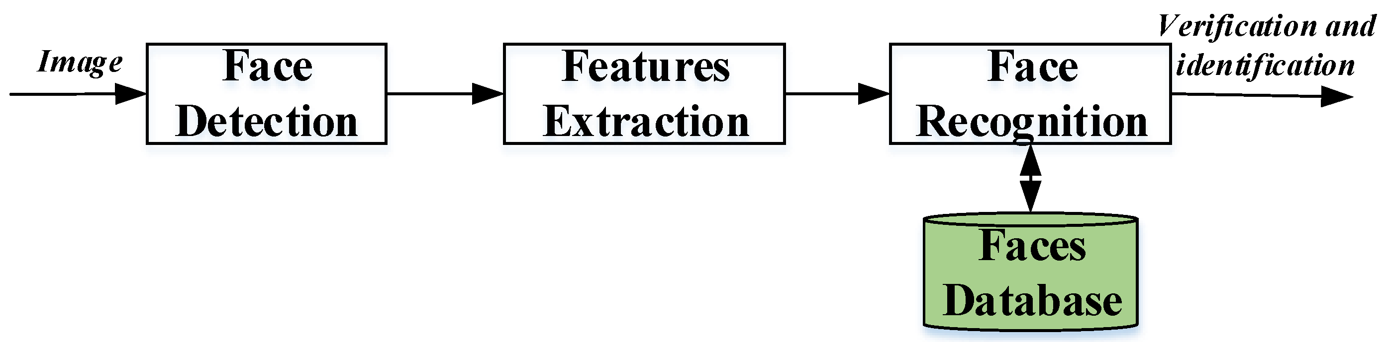
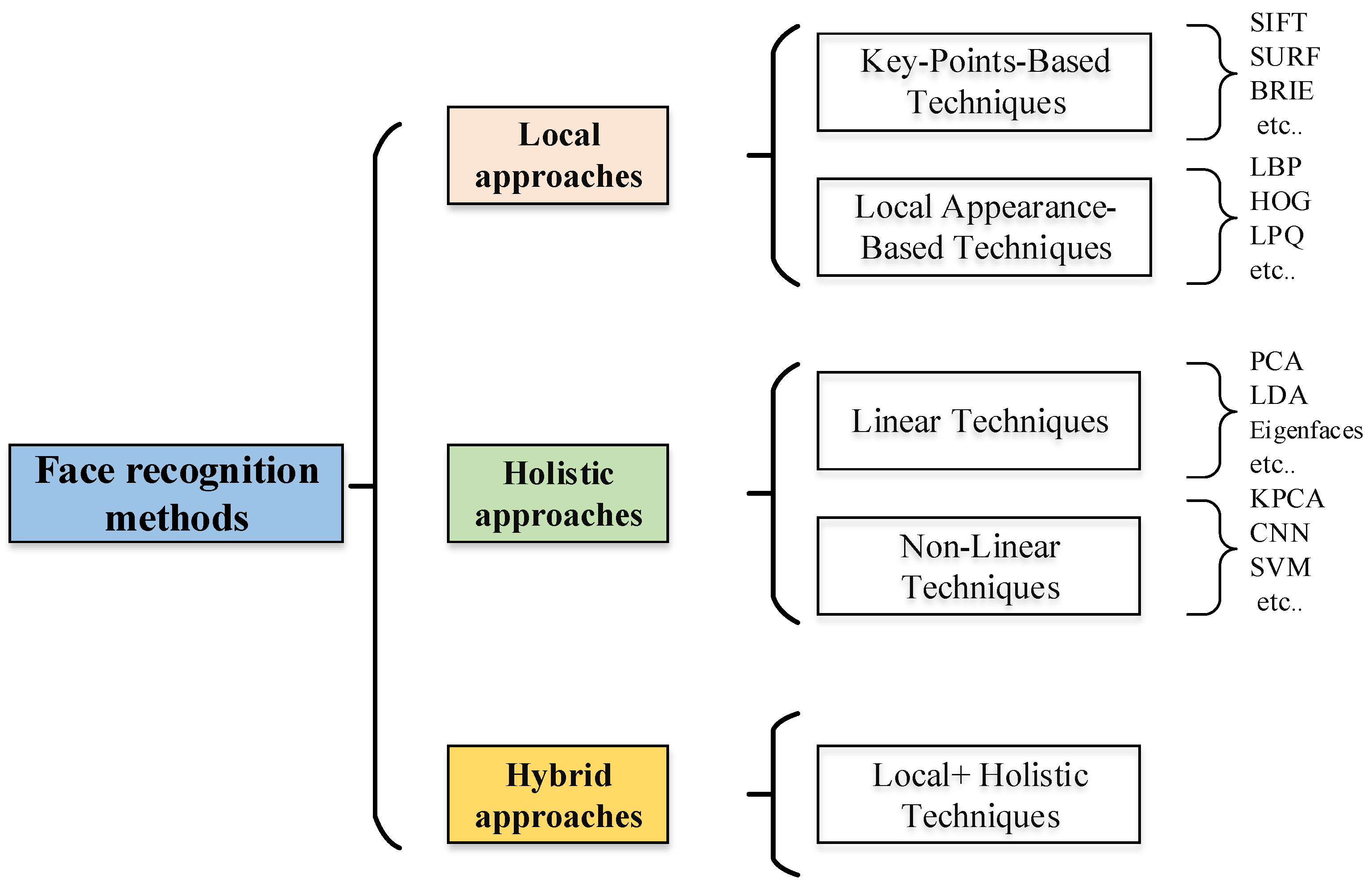
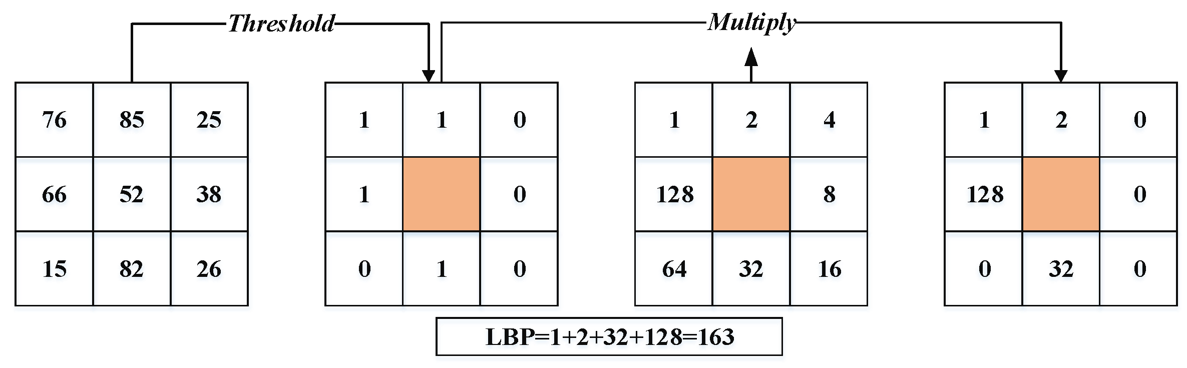
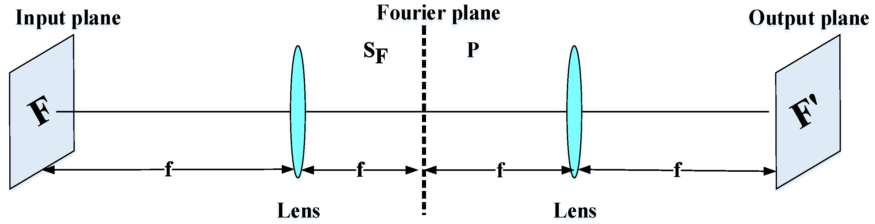
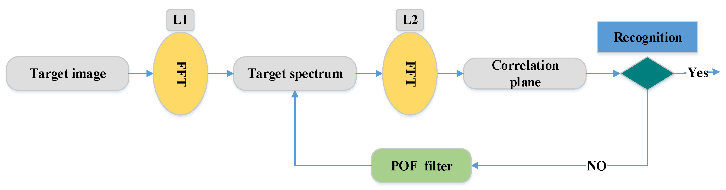
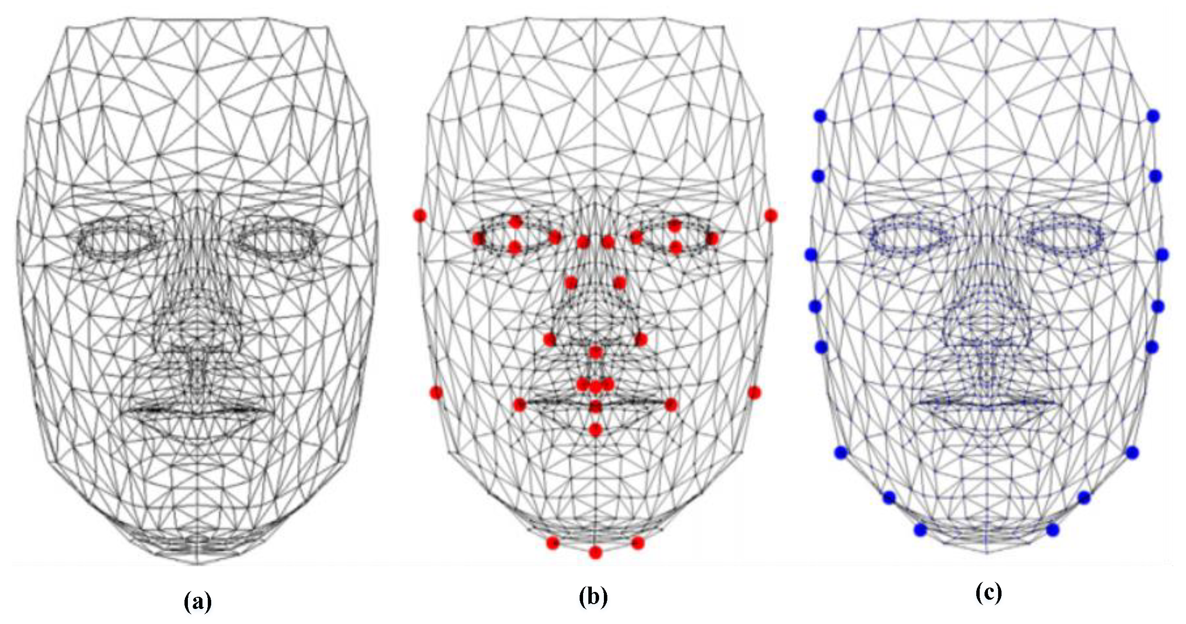
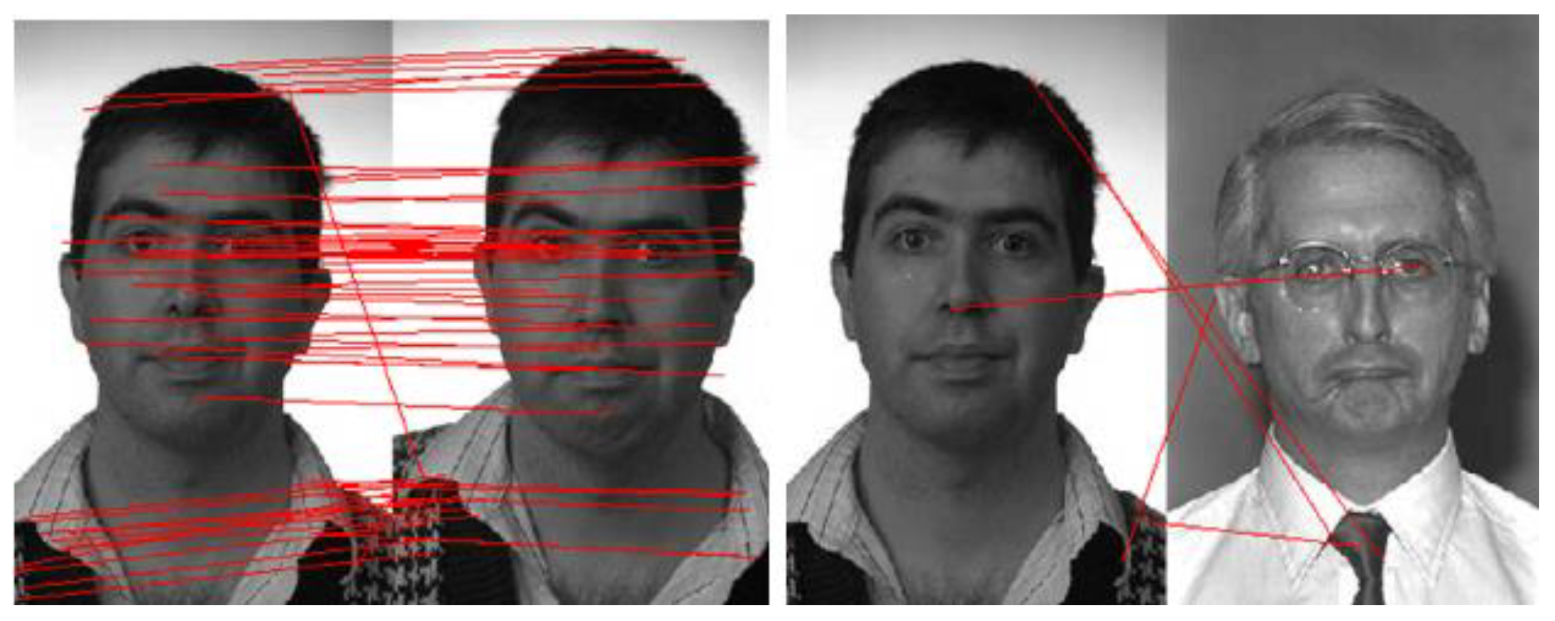
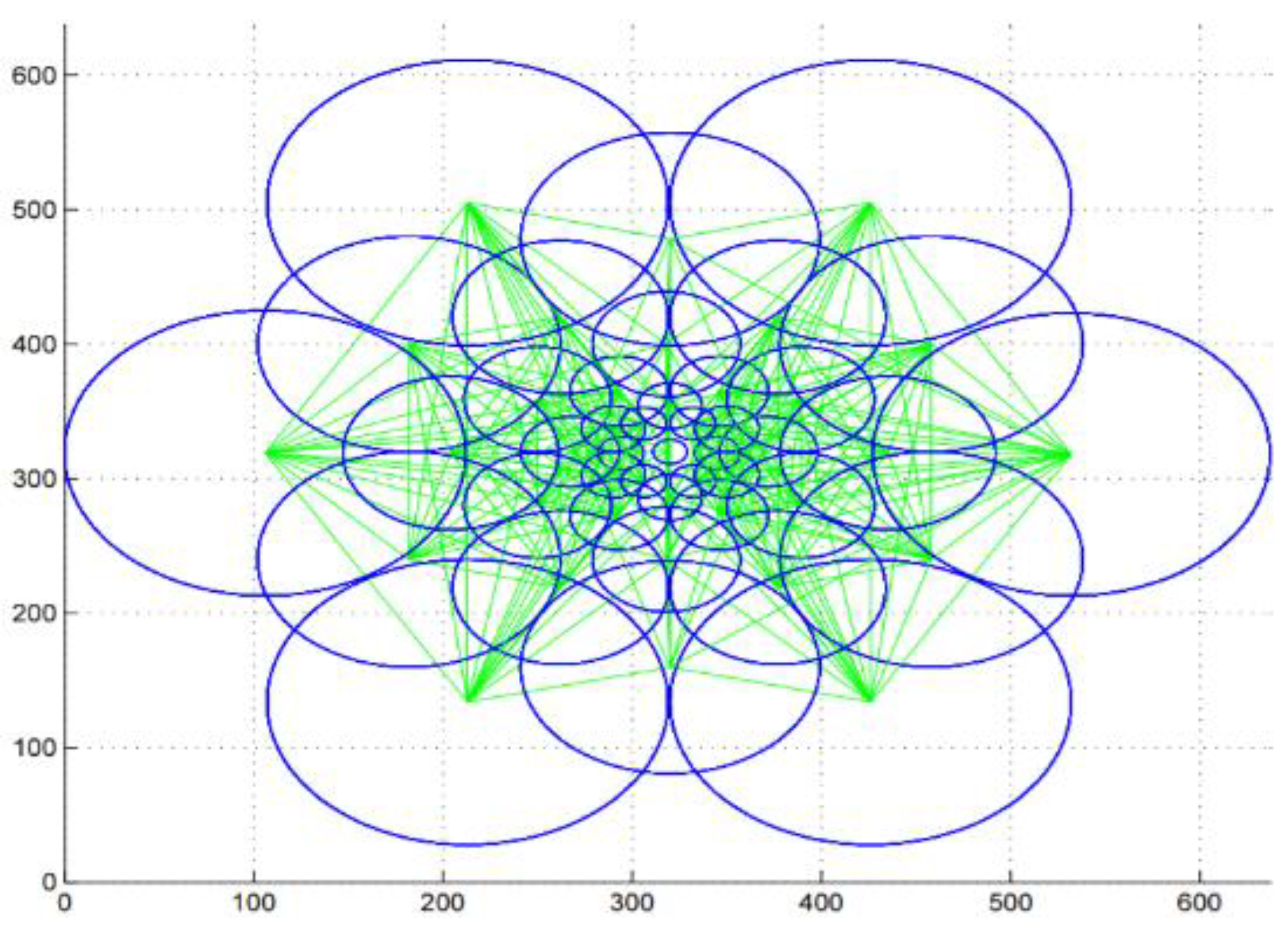
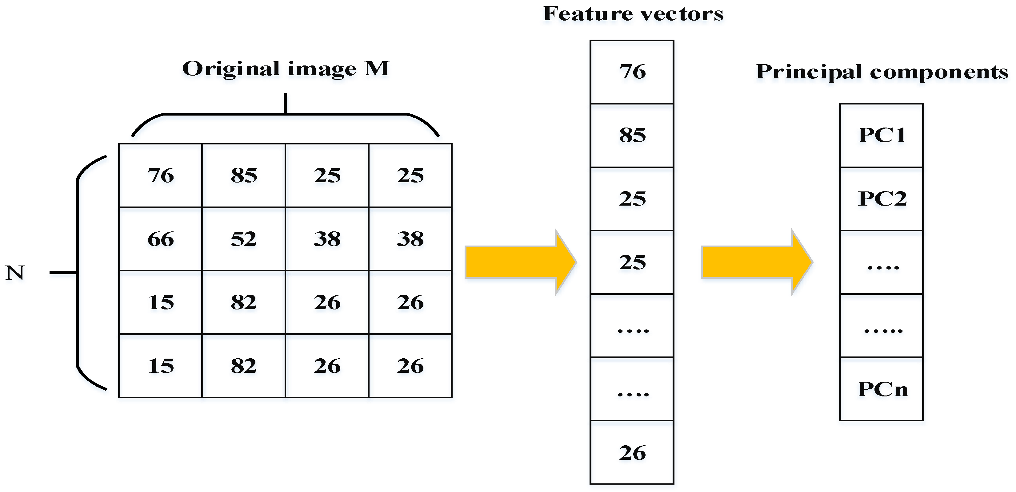
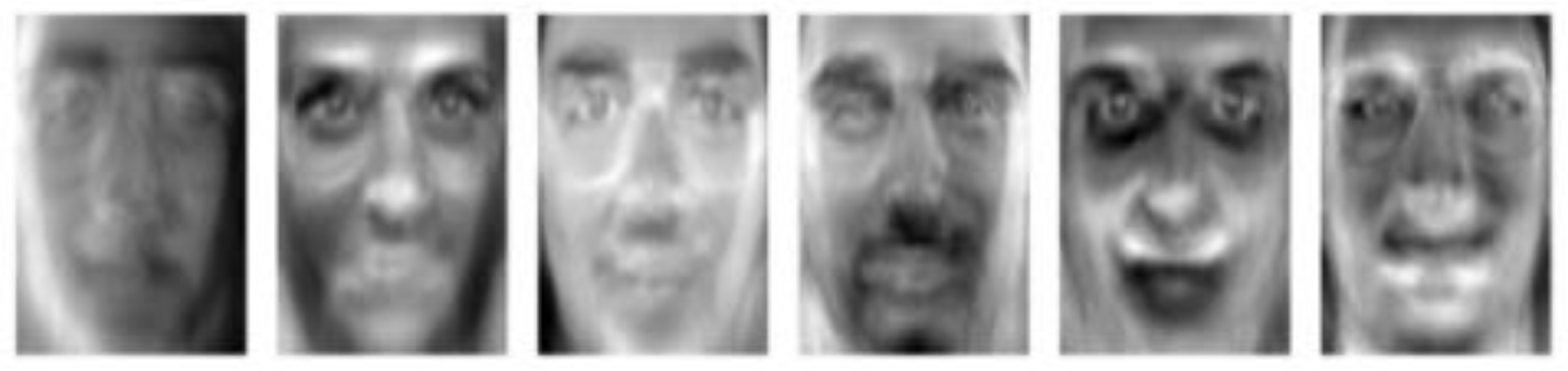
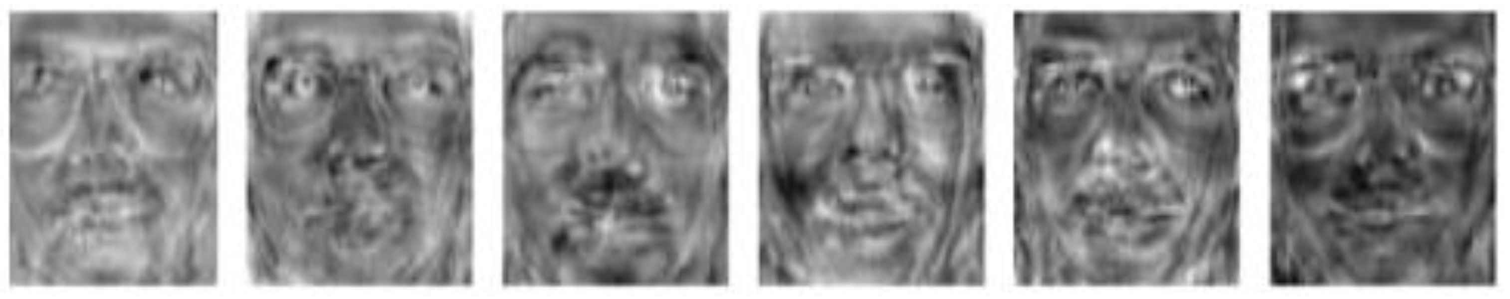
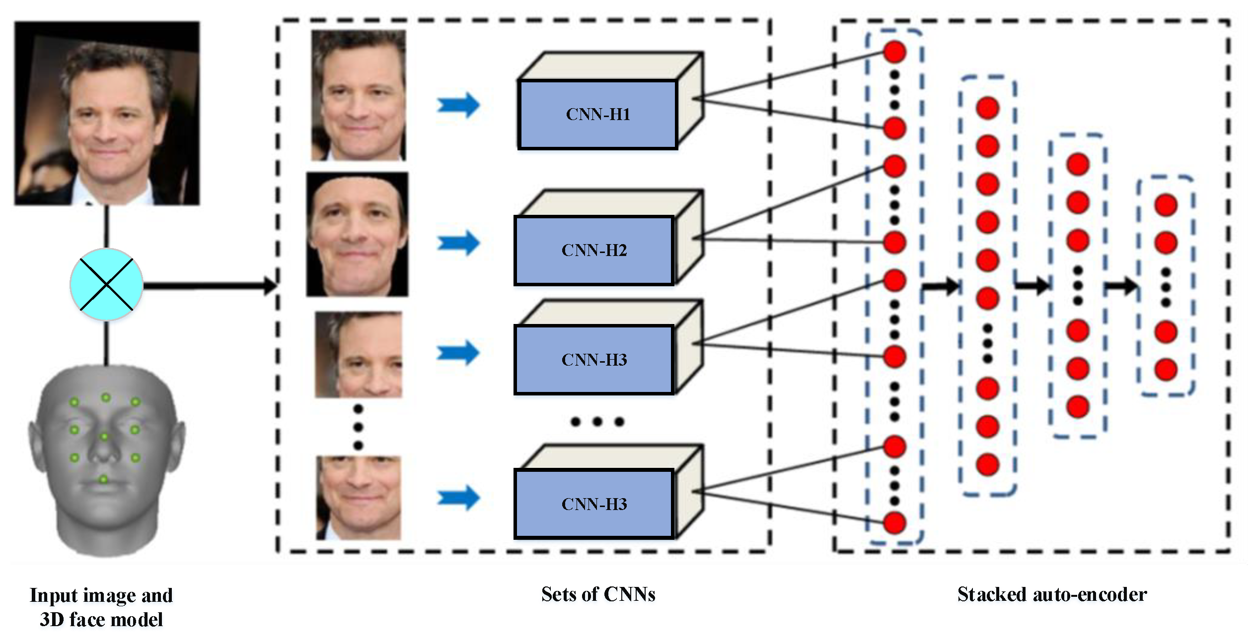
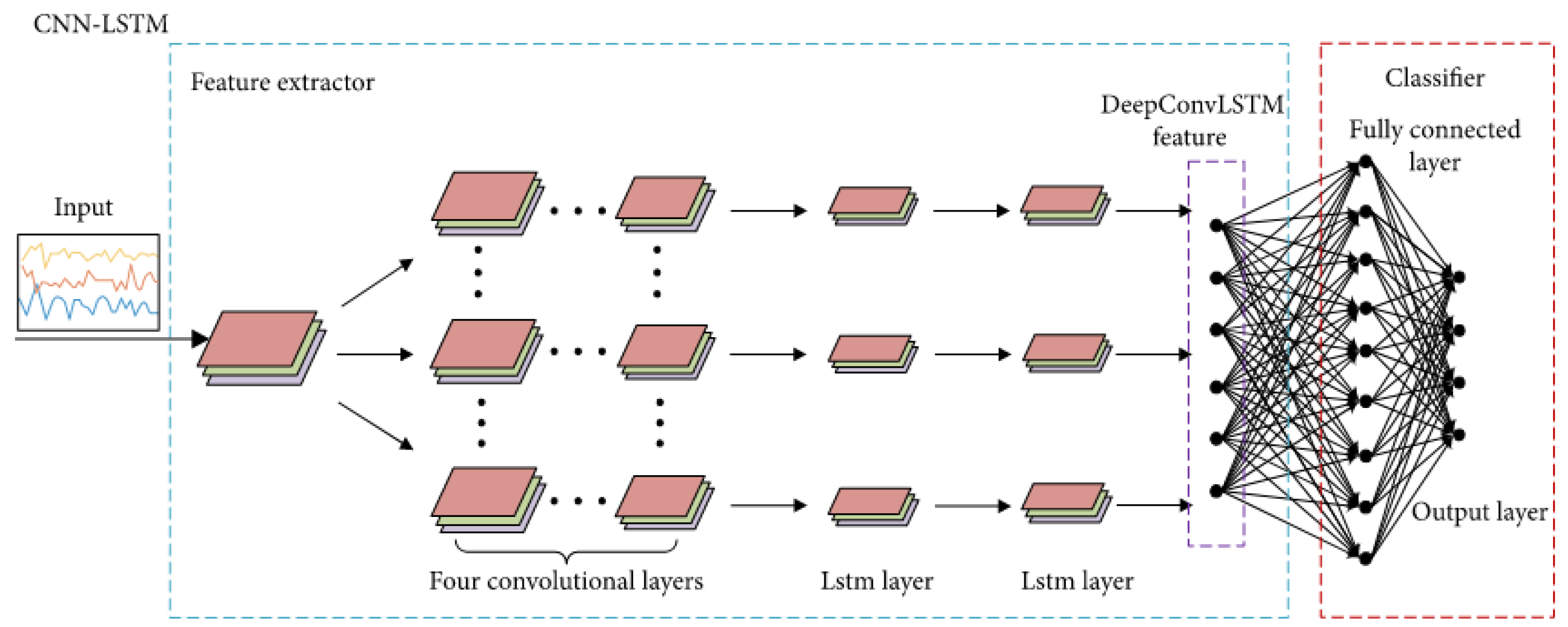
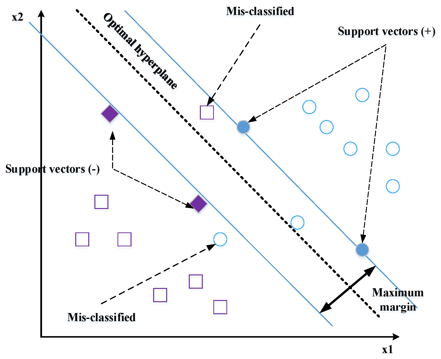
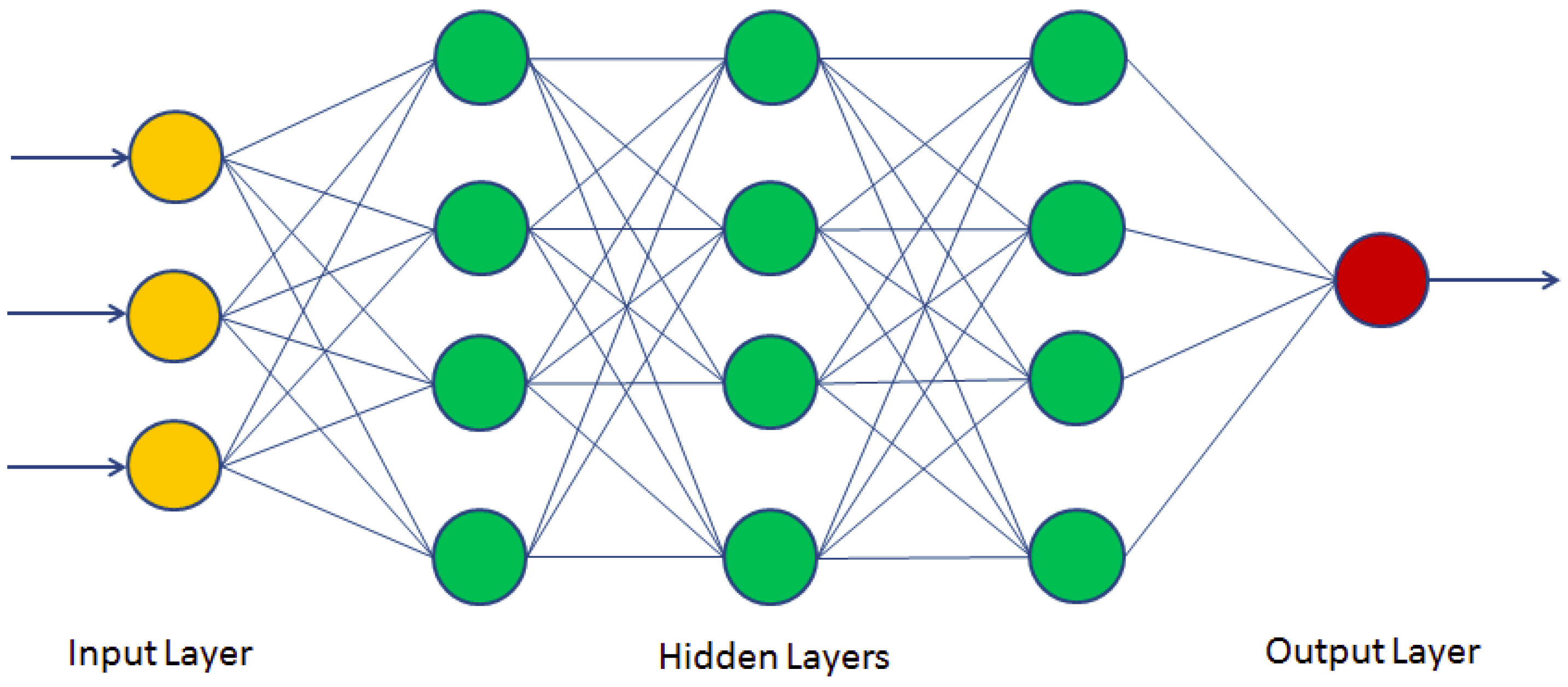
Table 1.
Summary of local approaches. SIFT, scale-invariant feature transform; SURF, scale-invariant feature transform; BRIEF, binary robust independent elementary features; LBP, local binary pattern; HOG, histogram of oriented gradients; LPQ, local phase quantization; PCA, principal component analysis; LDA, linear discriminant analysis; KPCA, kernel PCA; CNN, convolutional neural network; SVM, support vector machine; PLBP, pyramid of LBP; KNN, k-nearest neighbor; MLBP, multiscale LBP; LTP, local ternary pattern.; PHOG, pyramid HOG; VLC, VanderLugt correlator; LFW, Labeled Faces in the Wild; FERET, Face Recognition Technology; PHPID, Pointing Head Pose Image Database; PCE, peak to correlation energy; POF, phase-only filter; PSR, peak-to-sidelobe ratio.
| Author/Technique Used | Database | Matching | Limitation | Advantage | Result | |
|---|---|---|---|---|---|---|
| Local Appearance-Based Techniques | ||||||
| Khoi et al. [20] | LBP | TDF | MAP | Skewness in face image | Robust feature in fontal face | 5% |
| CF1999 | 13.03% | |||||
| LFW | 90.95% | |||||
| Xi et al. [15] | LBPNet | FERET | Cosine similarity | Complexities of CNN | High recognition accuracy | 97.80% |
| LFW | 94.04% | |||||
| Khoi et al. [20] | PLBP | TDF | MAP | Skewness in face image | Robust feature in fontal face | 5.50% |
| CF | 9.70% | |||||
| LFW | 91.97% | |||||
| Laure et al. [40] | LBP and KNN | LFW | KNN | Illumination conditions | Robust | 85.71% |
| CMU-PIE | 99.26% | |||||
| Bonnen et al. [42] | MRF and MLBP | AR (Scream) | Cosine similarity | Landmark extraction fails or is not ideal | Robust to changes in facial expression | 86.10% |
| FERET (Wearing sunglasses) | 95% | |||||
| Ren et al. [43] | Relaxed LTP | CMU-PIE | Chisquare distance | Noise level | Superior performance compared with LBP, LTP | 95.75% |
| Yale B | 98.71% | |||||
| Hussain et al. [60] | LPQ | FERET/ | Cosine similarity | Lot of discriminative information | Robust to illumination variations | 99.20% |
| LFW | 75.30% | |||||
| Karaaba et al. [44] | HOG and MMD | FERET | MMD/MLPD | Low recognition accuracy | Aligning difficulties | 68.59% |
| LFW | 23.49% | |||||
| Arigbabu et al. [46] | PHOG and SVM | LFW | SVM | Complexity and time of computation | Head pose variation | 88.50% |
| Leonard et al. [50] | VLC correlator | PHPID | ASPOF | The low number of the reference image used | Robustness to noise | 92% |
| Napoléon et al. [38] | LBP and VLC | YaleB | POF | Illumination | Rotation + Translation | 98.40% |
| YaleB Extended | 95.80% | |||||
| Heflin et al. [54] | correlation filter | LFW/PHPID | PSR | Some pre-processing steps | More effort on the eye localization stage | 39.48% |
| Zhu et al. [55] | PCA–FCF | CMU-PIE | Correlation filter | Use only linear method | Occlusion-insensitive | 96.60% |
| FRGC2.0 | 91.92% | |||||
| Seo et al. [27] | LARK + PCA | LFW | Cosine similarity | Face detection | Reducing computational complexity | 78.90% |
| Ghorbel et al. [61] | VLC + DoG | FERET | PCE | Low recognition rate | Robustness | 81.51% |
| Ghorbel et al. [61] | uLBP + DoG | FERET | chi-square distance | Robustness | Processing time | 93.39% |
| Ouerhani et al. [18] | VLC | PHPID | PCE | Power | Processing time | 77% |
| Key-Points-Based Techniques | ||||||
| Lenc et al. [56] | SIFT | FERET | a posterior probability | Still far to be perfect | Sufficiently robust on lower quality real data | 97.30% |
| AR | 95.80% | |||||
| LFW | 98.04% | |||||
| Du et al. [29] | SURF | LFW | FLANN distance | Processing time | Robustness and distinctiveness | 95.60% |
| Vinay et al. [23] | SURF + SIFT | LFW | FLANN | Processing time | Robust in unconstrained scenarios | 78.86% |
| Face94 | distance | 96.67% | ||||
| Calonder et al. [30] | BRIEF | _ | KNN | Low recognition rate | Low processing time | 48% |
Table 2.
Subspace approaches. ICA, independent component analysis; DWT, discrete wavelet transform; FFT, fast Fourier transform; DCT, discrete cosine transform.
Table 2.
Subspace approaches. ICA, independent component analysis; DWT, discrete wavelet transform; FFT, fast Fourier transform; DCT, discrete cosine transform.
| Author/Techniques Used | Databases | Matching | Limitation | Advantage | Result | |
|---|---|---|---|---|---|---|
| Linear Techniques | ||||||
| Seo et al. [27] | LARK and PCA | LFW | L2 distance | Detection accuracy | Reducing computational complexity | 85.10% |
| Annalakshmi et al. [35] | ICA and LDA | LFW | Bayesian Classifier | Sensitivity | Good accuracy | 88% |
| Annalakshmi et al. [35] | PCA and LDA | LFW | Bayesian Classifier | Sensitivity | Specificity | 59% |
| Hussain et al. [36] | LQP and Gabor | FERET | Cosine similarity | Lot of discriminative information | Robust to illumination variations | 99.2% 75.3% |
| LFW | ||||||
| Gowda et al. [17] | LPQ and LDA | MEPCO | SVM | Computation time | Good accuracy | 99.13% |
| Z. Cui et al. [67] | BoW | AR | ASM | Occlusions | Robust | 99.43% |
| ORL | 99.50% | |||||
| FERET | 82.30% | |||||
| Khan et al. [83] | PSO and DWT | CK | Euclidienne distance | Noise | Robust to illumination | 98.60% |
| MMI | 95.50% | |||||
| JAFFE | 98.80% | |||||
| Huang et al. [70] | 2D-DWT | FERET | KNN | Pose | Frontal or near-frontal facial images | 90.63% 97.10% |
| LFW | ||||||
| Perlibakas and Vytautas [69] | PCA and Gabor filter | FERET | Cosine metric | Precision | Pose | 87.77% |
| Hafez et al. [84] | Gabor filter and LDA | ORL | 2DNCC | Pose | Good recognition performance | 98.33% |
| C. YaleB | 99.33% | |||||
| Sufyanu et al. [71] | DCT | ORL | NCC | High memory | Controlled and uncontrolled databases | 93.40% |
| Yale | ||||||
| Shanbhag et al. [85] | DWT and BPSO | _ _ | _ _ | Rotation | Significant reduction in the number of features | 88.44% |
| Ghorbel et al. [61] | Eigenfaces and DoG filter | FERET | Chi-square distance | Processing time | Reduce the representation | 84.26% |
| Zhang et al. [12] | PCA and FFT | YALE | SVM | Complexity | Discrimination | 93.42% |
| Zhang et al. [12] | PCA | YALE | SVM | Recognition rate | Reduce the dimensionality | 84.21% |
| Nonlinear Techniques | ||||||
| Fan et al. [86] | RKPCA | MNIST ORL | RBF kernel | Complexity | Robust to sparse noises | _ |
| Vinay et al. [87] | ORB and KPCA | ORL | FLANN Matching | Processing time | Robust | 87.30% |
| Vinay et al. [87] | SURF and KPCA | ORL | FLANN Matching | Processing time | Reduce the dimensionality | 80.34% |
| Vinay et al. [87] | SIFT and KPCA | ORL | FLANN Matching | Low recognition rate | Complexity | 69.20% |
| Lu et al. [88] | KPCA and GDA | UMIST face | SVM | High error rate | Excellent performance | 48% |
| Yang et al. [89] | PCA and MSR | HELEN face | ESR | Complexity | Utilizes color, gradient, and regional information | 98.00% |
| Yang et al. [89] | LDA and MSR | FRGC | ESR | Low performances | Utilizes color, gradient, and regional information | 90.75% |
| Ouanan et al. [90] | FDDL | AR | CNN | Occlusion | Orientations, expressions | 98.00% |
| Vankayalapati and Kyamakya [77] | CNN | ORL | _ _ | Poses | High recognition rate | 95% |
| Devi et al. [63] | 2FNN | ORL | _ _ | Complexity | Low error rate | 98.5 |
Table 3.
Hybrid approaches. GW, Gabor wavelet; OCLBP, over-complete LBP; WCCN, within class covariance normalization; WLBP, Walsh LPB; ICP, iterative closest point; LGBPHS, local Gabor binary pattern histogram sequence; FLD, Fisher linear discriminant; SAE, stacked auto-encoder.
Table 3.
Hybrid approaches. GW, Gabor wavelet; OCLBP, over-complete LBP; WCCN, within class covariance normalization; WLBP, Walsh LPB; ICP, iterative closest point; LGBPHS, local Gabor binary pattern histogram sequence; FLD, Fisher linear discriminant; SAE, stacked auto-encoder.
| Author/Technique Used | Database | Matching | Limitation | Advantage | Result | |
|---|---|---|---|---|---|---|
| Fathima et al. [91] | GW-LDA | AT&T | k-NN | High processing time | Illumination invariant and reduce the dimensionality | 88% |
| FACES94 | 94.02% | |||||
| MITINDIA | 88.12% | |||||
| Barkan et al., [92] | OCLBP, LDA, and WCCN | LFW | WCCN | _ | Reduce the dimensionality | 87.85% |
| Juefei et al. [93] | ACF and WLBP | LFW | Complexity | Pose conditions | 89.69% | |
| Simonyan et al. [64] | Fisher + SIFT | LFW | Mahalanobis matrix | Single feature type | Robust | 87.47% |
| Sharma et al. [96] | PCA–ANFIS | ORL | ANFIS | Sensitivity-specificity | 96.66% | |
| ICA–ANFIS | ANFIS | Pose conditions | 71.30% | |||
| LDA–ANFIS | ANFIS | 68% | ||||
| Ojala et al. [97] | DCT–PCA | ORL | Euclidian distance | Complexity | Reduce the dimensionality | 92.62% |
| UMIST | 99.40% | |||||
| YALE | 95.50% | |||||
| Mian et al. [98] | Hotelling transform, SIFT, and ICP | FRGC | ICP | Processing time | Facial expressions | 99.74% |
| Cho et al. [99] | PCA–LGBPHS | Extended Yale Face | Bhattacharyya distance | Illumination condition | Complexity | 95% |
| PCA–GABOR Wavelets | ||||||
| Sing et al. [101] | PCA–FLD | CMU | SVM | Robustness | Pose, illumination, and expression | 71.98% |
| FERET | 94.73% | |||||
| AR | 68.65% | |||||
| Kamencay et al. [102] | SPCA-KNN | ESSEX | KNN | Processing time | Expression variation | 96.80% |
| Sun et al. [103] | CNN–LSTM–ELM | OPPORTUNITY | LSTM/ELM | High processing time | Automatically learn feature representations | 90.60% |
| Ding et al. [95] | CNNs and SAE | LFW | _ _ | Complexity | High recognition rate | 99% |
Table 4.
General performance of face recognition approaches.
| Approaches | Databases Used | Advantages | Disadvantages | Performances | Challenges Handled | |
|---|---|---|---|---|---|---|
| Local | Local Appearance | TDF, CF1999, LFW, FERET, CMU-PIE, AR, Yale B, PHPID, YaleB Extended, FRGC2.0, Face94. |
|
| ||
| Key-Points |
|
| ||||
| Holistic | Linear | LFW, FERET, MEPCO, AR, ORL, CK, MMI, JAFFE, C. Yale B, Yale, MNIST, ORL, UMIST face, HELEN face, FRGC. |
|
| ||
| Non-Linear |
|
|
| |||
| Hybrid | AT&T, FACES94, MITINDIA, LFW, ORL, UMIST, YALE, FRGC, Extended Yale, CMU, FERET, AR, ESSEX. |
|
| |||
© 2020 by the authors. Licensee MDPI, Basel, Switzerland. This article is an open access article distributed under the terms and conditions of the Creative Commons Attribution (CC BY) license (http://creativecommons.org/licenses/by/4.0/).
Share and Cite
MDPI and ACS Style
Kortli, Y.; Jridi, M.; Al Falou, A.; Atri, M. Face Recognition Systems: A Survey. Sensors 2020, 20, 342. https://doi.org/10.3390/s20020342
AMA Style
Kortli Y, Jridi M, Al Falou A, Atri M. Face Recognition Systems: A Survey. Sensors. 2020; 20(2):342. https://doi.org/10.3390/s20020342
Chicago/Turabian StyleKortli, Yassin, Maher Jridi, Ayman Al Falou, and Mohamed Atri. 2020. "Face Recognition Systems: A Survey" Sensors 20, no. 2: 342. https://doi.org/10.3390/s20020342
Note that from the first issue of 2016, this journal uses article numbers instead of page numbers. See further details here.