Article

Performance of a Low-Cost Sensor Community Air Monitoring Network in Imperial County, CA

1
Dept. of Public Health, Richmond, CA 94804, USA
2
Tracking California, Public Health Institute, Oakland, CA 94607, USA
3
Comite Civico Del Valle, Brawley, CA 92227, USA
4
Environmental and Occupational Health Sciences, University of Washington, Seattle, WA 98195, USA
5
Department of Environmental Health Sciences, School of Public Health, University of California, Los Angeles, CA 90097, USA
6
Department of Environmental and Occupational Health, George Washington University, Washington, DC 20037, USA
*
Author to whom correspondence should be addressed.
Sensors 2020, 20(11), 3031; https://doi.org/10.3390/s20113031
Submission received: 11 May 2020 / Revised: 21 May 2020 / Accepted: 25 May 2020 / Published: 27 May 2020
(This article belongs to the Section State-of-the-Art Sensors Technologies)

Abstract

:
Air monitoring networks developed by communities have potential to reduce exposures and affect environmental health policy, yet there have been few performance evaluations of networks of these sensors in the field. We developed a network of over 40 air sensors in Imperial County, CA, which is delivering real-time data to local communities on levels of particulate matter. We report here on the performance of the Network to date by comparing the low-cost sensor readings to regulatory monitors for 4 years of operation (2015–2018) on a network-wide basis. Annual mean levels of PM10 did not differ statistically from regulatory annual means, but did for PM2.5 for two out of the 4 years. R2s from ordinary least square regression results ranged from 0.16 to 0.67 for PM10, and increased each year of operation. Sensor variability was higher among the Network monitors than the regulatory monitors. The Network identified a larger number of pollution episodes and identified under-reporting by the regulatory monitors. The participatory approach of the project resulted in increased engagement from local and state agencies and increased local knowledge about air quality, data interpretation, and health impacts. Community air monitoring networks have the potential to provide real-time reliable data to local populations.

1. Introduction

Small, low-cost air quality sensors of improving quality are becoming increasing available, and many public health and research projects are now employing these next-generation air monitors to conduct personal and local-level air monitoring for exposure control [1,2]. This new technology holds great potential to address gaps in regulatory air monitoring data to better characterize air quality at the community level. With the stall of international agreements to decrease emissions to address climate change, local community networks could result in cost-effective improvements to air monitoring and emission reduction at the local scale in the near-term and have policy relevance and positive developments globally for climate change and air pollution in the long-term. Starting in 2014, the Imperial County Community Air Monitoring Network (“the Network”) has combined community participatory and scientific methods to develop a network of over 40 air sensors throughout the county, delivering real-time data to local communities on levels of particulate matter. The Network now has 4 years of data available for performance evaluation. Although the use of these sensors is increasing, there have been few performance evaluations of low-cost networks operating in the field [3,4] and none which have reported with such extensive data. Duvall et al. [3] evaluated the performance of low-cost sensors measuring NO2 and ozone in two U.S. cities, and found good agreement of their sensors with reference sites. Mailings et al. [4] developed a low-cost gas sensor and evaluated multiple statistical methods for evaluating sensor performance. In Salerno, Italy, Sofia et al. [5] evaluated the performance of a low-cost network measuring PM2.5 and found good agreement of their sensors with gravimetric sampling. Although there have been calibration/validation studies of these sensors, to our knowledge no studies have been conducted evaluating performance of a low-cost network post implementation on a network-wide basis, compared to regulatory data. Further, none of the previous evaluations have been done on community-based air monitoring systems where the community has taken the lead in monitor siting and hardware/software maintenance of the network.
We have previously reported on the monitor calibration/validation [6], and the process for monitor siting [7]. The objective of this paper is to evaluate the performance of the Network to date by comparing the low-cost sensor readings to regulatory monitors for 4 years of operation (2015–2018) on a network/domain-wide basis. We also discuss how the participatory research approach affected the project overall, and the policy and public health actions which have resulted from the project.

2. Materials and Methods

Imperial County, CA, is home to a primarily Latino population (84%) and has some of the highest rates of unemployment (47%) and poverty (24%) in the nation [8]. The county is primarily a desert ecosystem, much of which has been converted to agricultural land. The county has a range of air pollution sources that contribute to regular and sustained exceedances of the California PM standards [9,10], including nearly 8 million vehicles annually crossing the U.S.-Mexico border in Calexico [11], an average of about 28,000 acres of agricultural field burned annually [12], and the drying Salton Sea [13].
The Imperial County Community Air Monitoring Network (the Network) was formed by a collaborative group of community, academic, nongovernmental, and government partners designed to fill the need for more detailed data on particulate matter in an area that often exceeds air quality standards. The Network employed a community-based environmental monitoring process in which community members and researchers had specific, well-defined roles as part of an equitable partnership that also includes shared decision-making to determine study direction, plan research protocols, and conduct project activities. Community members played key roles in determining study design, siting and deploying monitors, and data collection. The Network is now producing real-time particulate matter data from 42 low-cost sensors throughout the county. The Network is one of the largest community-based air monitoring networks in the U.S. and, to our knowledge, is the first community-designed network of its size in the world.
The project partners included Comite Civico del Valle (CCV), a community-based organization in Imperial County; Tracking California, a program of the nongovernmental Public Health Institute in collaboration with the CA Department of Public Health; and the Seto research group at the University of Washington (UW). Faculty at the University of California at Los Angeles and George Washington University served in an advisory capacity. The distinct roles of the partners and the initial community engagement structure have been described in detail elsewhere [14].
The monitor selected for the Network was a modified laser-based optical counter (Dylos DC1700, Dylos Corpration, Riverside, CA, USA). The firmware was changed to increase the number of particle size bins from two to four (>0.5, >1.0, >2.5, and >10 μm). Particle counts were converted to mass concentrations to align with health recommendations that are usually based on the latter. Algorithms to convert counts to mass were developed, taking into account relative humidity, based on co-location of the instruments with federal equivalent method (FEM), beta-attenuation monitors (BAMs), and federal reference method (FRM) gravimetric filters. The algorithm, process for the calibration, and field validation, and further specifications of the Dylos monitor have been described in detail elsewhere [6].
The monitor system included the Dylos particle sensor, temperature and relative humidity sensors, a heater and fan, and a microcontroller to allow wireless real-time data transfer to the Internet. Data are sampled once every 10 s from the Dylos and a HIH6130 temperature and humidity sensor. Power consumption is about 3 W without the fan or heater (temp above 120 F), and 203 W with the heater and no fan (temp below 40 F). The monitor components were housed in a NEMA-6 rated enclosure with a cooling fan to sustain optimal sensor performance under Imperial County’s harsh summer conditions. The rationale and siting for the first 40 sensors were based on a two stage process where the community selected the locations of the first 20 sensors primarily based on locations of vulnerable populations and the second 20 based on specifications to meet the spatial requirements for land use regression [7]. We developed a process to involve community residents to select monitoring sites, which involved the use of mobile devices equipped with a custom-designed mobile web form, modified from IVAN Imperial (https://ivan-imperial.org/air), CCV’s existing community environmental reporting website [7]. Residents used government-based monitor siting criteria (such as building height, security, likelihood of available Wi-Fi and AC power supply, and locations of nearby air pollution sources) in their assessment.
The air quality data are transmitted in real-time to data servers managed by CCV once every 10 s (data are averaged every 5 min), converted from particle counts to mass concentrations, checked for quality assurance/quality control, and then fed to the IVAN website. Quality control procedures include flagging unusually low values, data completeness, and routine manual inspection of the sensors. The IVAN website developed by CCV allows public access to real-time data from the Network. The U.S. EPA Air Quality Index (AQI) is calculated for five major air pollutants regulated by the Clean Air Act: ozone, particulate matter, carbon monoxide, sulfur dioxide, and nitrogen dioxide [15]. As this project was only measuring particulate matter, another index was needed. To address this, the particle mass results (in μg/m3) were averaged using the U.S. EPA NowCast method [16]. The NowCast method produces a value for PM10 and PM2.5, which is an average of the previous 12 h. If the air quality that day is stable, then the hours are weighted more evenly (approaching a 12-h average). If the air quality that day is changing, then recent hours are weighted more heavily (approaching an average of the most recent 3-h). The resulting NowCast value (in μg/m3) is then converted to a Community Air-Quality Level (CAL)—an indicator developed specifically for this Network with community input—using the U.S. EPA Air Quality Index calculation method. After consultation with the Imperial Community Steering Committee on how to make the data most understandable and useable, CALs were categorized into four categories: green/low risk (0–50), yellow/moderate risk (51–100), orange/unhealthy for sensitive groups (101–150), and red/unhealthy (above 150). The CALs are calculated for each monitor based on current concentrations, with the number and category updated on this website every 5 min. The 30-day and 90-day summary statistics for CALs are calculated using 24-h AQIs.
To compare the overall daily averages of PM10 and PM2.5 from the Network versus regulatory monitors, we used reference monitor data available from U.S. EPA’s Air Quality System (https://www.epa.gov/aqs), which shows ambient air quality data reported to U.S. EPA by the State of California. We then matched Network and regulatory monitors by reporting day and computed mean 24-h averages across all Network sites (n = 42) and regulatory sites in the Imperial Valley (n = 5 for PM10, and n = 3 for PM2.5—two of the PM10 sites do not measure PM2.5). We then computed seasonal and annual averages from the mean 24-h averages. Daily averages for Network monitors were calculated from hourly averages with 75% completeness (nine 5-min measures or more per hour). Only 24-h averages for Network monitors with 75% completeness (18 h or more per day) were included in this analysis.
To test for significant differences in annual averages between Network and regulatory monitors, we conducted two-sample t-tests for independence with unequal variance in OpenEpi, Version 3 (https://www.OpenEpi.com). Two-sided p-values indicated significance at the α = 0.05 level. We used restricted maximum likelihood estimation to calculate unbiased inter- and intra-monitor variance estimates from monitor-specific 24-h measurements. We ran ordinary least squares (OLS) simple linear regressions to estimate associations between mean 24-h averages from all Network monitors and mean 24-h averages from all regulatory monitors, by pollutant and year. To reduce bias in our estimates which were calculated from aggregated data, we used the bootstrapping approach with n = 1000 random samples from the observed data, with replacement. This method yields robust estimates of variance and bias-corrected 95% confidence intervals.
We computed Lin’s concordance correlation coefficient for agreement. This method combines measures of precision and accuracy to determine how far the observed data (measured by two different methods) deviate from the 45° line of perfect concordance. Data were processed and analyzed in R, Version 3.6.1 (R Foundation for Statistical Computing, Vienna, Austria) using nmle() (Pinheiro J, Bates D, DebRoy S, Sarkar D and R Core Team, 2016), boot() (Canty A, Ripley BD, 2020), ggplot2() (Wickham H, 2016), and agRee() (Feng D, 2020) packages for inter- and intra-monitor variance estimation, bootstrapping and regression plots, and concordance correlation coefficient estimation.

3. Results

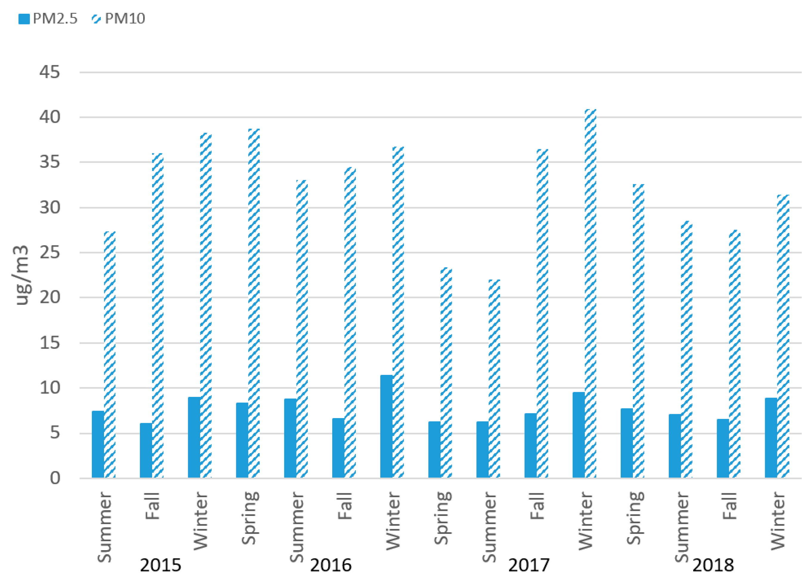
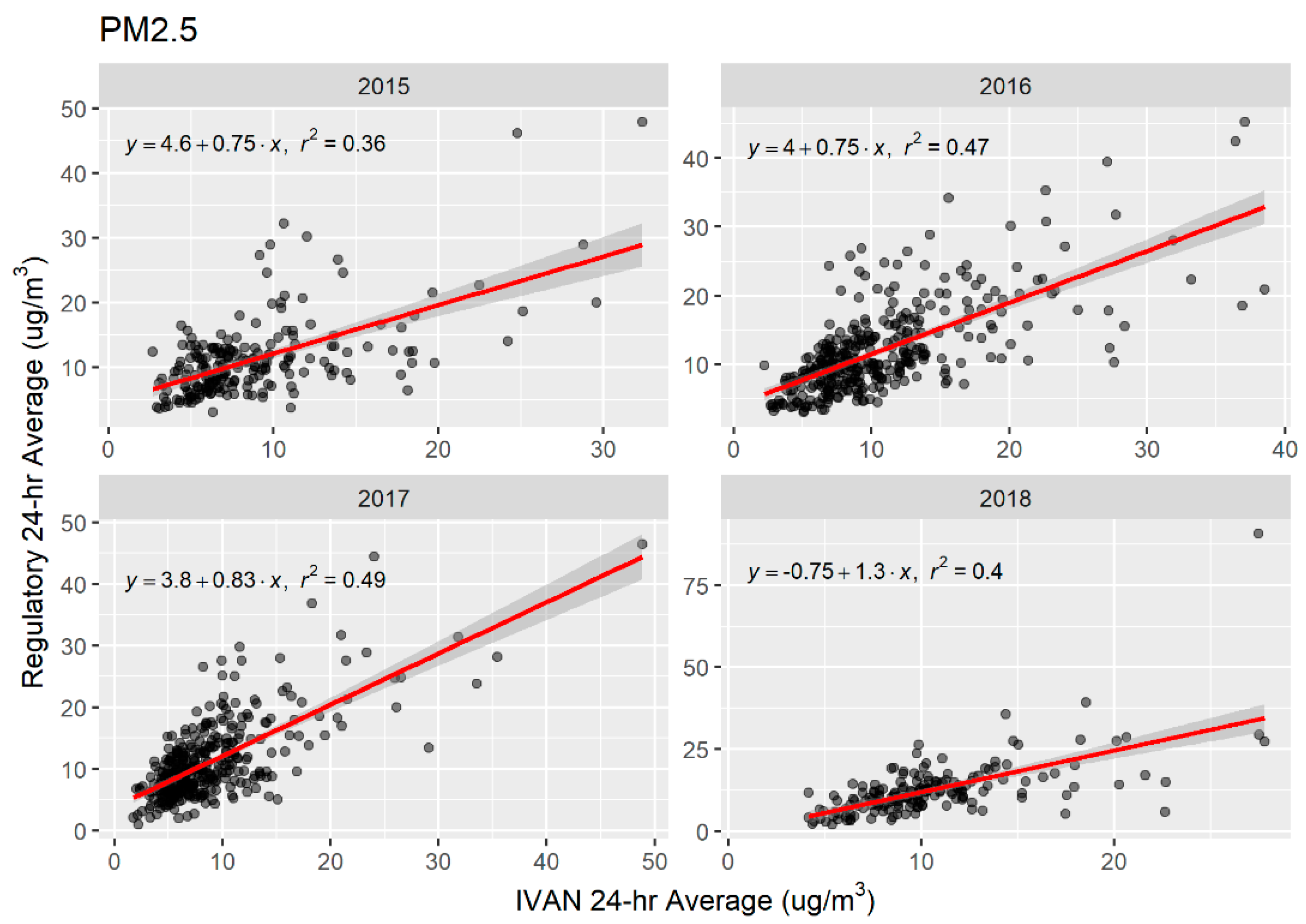
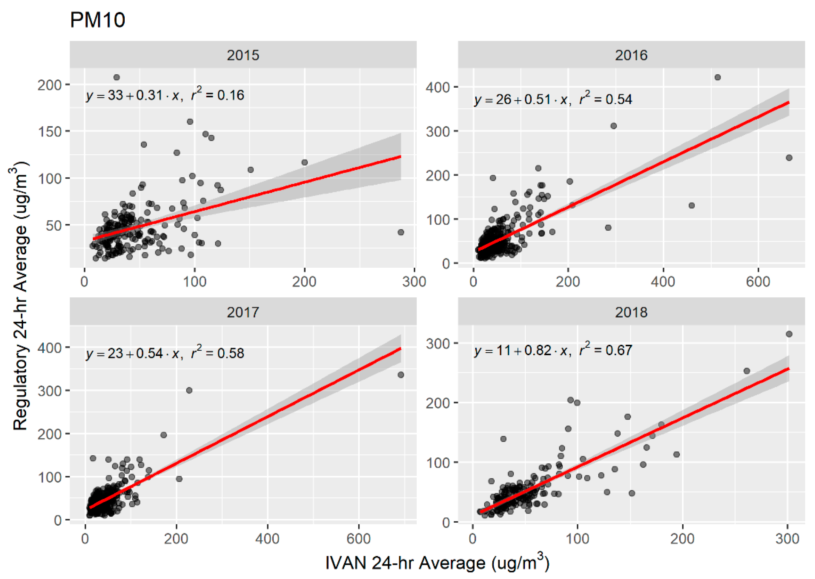
3.1. Air Quality Results

After removing incomplete hourly and daily averages, there were 28,782 and 21,675 daily average values from 42 Network monitors between 29 May 2015 and 30 June 2018 for PM2.5 and PM10, respectively. In the same time period, there were 1767 PM2.5 daily averages from three regulatory monitors and 4858 PM10 daily averages from five regulatory monitors. After aggregating across monitor sites, we analyzed 1053 and 1051 paired Network-regulatory mean 24-h averages for PM2.5 and PM10, respectively.
Figure 1 shows median annual 24-h average PM2.5 and PM10 values from the Network during the 2015–2018 period. Median PM2.5 levels from the Network appear to be highest in winter, but there was no overall trend in increasing levels by time (Figure 1). Average 24-h PM2.5 values ranged from <1 to 255 μg/m3 during the time period. PM10 values also were highest in winter (Figure 1), except for Spring 2016 being the highest for that year. PM10 values ranged from 1.8 to 2431 μg/m3.
Table 1 shows average annual 24-h values of PM2.5 and PM10 from the Network and from CA regulatory sites in the Imperial Valley from 2015 to 2018 on a network-average basis. Mean values were not statistically significant for any year for PM10, but were statistically different for PM2.5 for 2015 and 2017. Data variability overall was much larger in the Network compared to the regulatory monitors, indicated by higher standard deviations, particularly for PM10. The 24-h average maximum levels of PM10 recorded by the community air Network reached 2430 μg/m3 in 2017 and the maximum level of 24-h mean of PM2.5 was 255 μg/m3 in 2018 (not shown).
Annual average PM2.5 measurements of the Network were consistently lower than those from regulatory monitors. These differences were only statistically significant in 2015 (t = 4.78, p < 0.0001) and 2017 (t = 3.56, p = 0.0004). This could possibly be explained by the fact that most of the regulatory monitors are located in more urban areas which would have higher levels of PM2.5, compared to the more diverse locations of the community monitors, or that the Dylos sensors are measuring PM10 more accurately than PM2.5. Community average annual levels of PM10 were not consistently higher or lower than the regulatory monitor average annual readings.
Monitor-specific 24-h averages were used to estimate variance between and within monitors for both Network and regulatory monitors, shown in Table 2. Inter-monitor variance was higher in the Network compared to that of regulatory monitors, suggesting greater variability across monitor locations in the Network. Intra-monitor variance was also higher in the Network, suggesting greater variability within each monitor location across time. Overall, intra-monitor variance was higher than inter-monitor variance for both Network and regulatory monitors, except for PM2.5 measurements from Network monitors which had greater variance between monitors than within.
Scatter plots and OLS linear regression lines for PM2.5 and PM10 are shown in Figure 2 and Figure 3, respectively. Network and regulatory mean daily averages were significantly associated for both PM2.5 and PM10 across all years. Linear associations were weak to moderate, as indicated by r-squared values, and robust estimates of standard error were low (Table 3). For PM2.5, regression lines show that Network monitors are, on average, predicting similar mean 24-h averages as the regulatory monitors. For PM10, regression lines show that predicted mean 24-h averages for Network monitors are similar to those of the regulatory monitors when estimates are less than 100 μg/m3. However, Network monitors are predicted to have higher mean 24-h averages for measures of PM10 in the range of 200–600 μg/m3 compared to predicted values for regulatory monitors.
Concordance coefficients indicate moderate agreement between Network and regulatory 24-h averages (Table 4). Agreement was similar for measurements of PM10 (Rho = 0.692, CI = 0.661, 0.720) and PM2.5 (Rho = 0.604, CI = 0.567, 0.638).

3.2. Under-Reporting by Government Monitors

In the beginning of 2016, the CA Air Resources Board began continuous PM10 monitoring at Calexico, CA in the Imperial Valley with a BAM FEM. The default setting of the BAM was capped at 985 μg/m3. Episodes examined in May of 2016 and October of 2017 showed while the FEM BAM showed values of “985,” the Dylos monitors were reporting readings exceeding 1800 and 1600 μg/m3, respectively [17]. Upon consultation with the U.S. EPA, CARB examined data from a collocated Dylos PM sensor from the Imperial Community Air Network for comparison. In December 2017, the FEM PM10 BAM was re-ranged by CARB to measure up to 4985 μg/m3. This correction will have an impact on historic and current average and maximum PM10 values.

3.3. Network Maintenance

Establishment of the Network has given the study partners the opportunity to learn and explore various issues with emerging low-cost sensor technology. The Imperial Community Air Monitoring Network has been running longer than other monitoring networks of its type, which are typically deployed for research purposes for a couple of months to a year. Through the study period, efforts were made to transfer knowledge, ownership and monitoring activities to CCV. All field maintenance tasks are currently managed by CCV staff, some who received training at the UW lab, and all hardware designs and software code were provided to CCV. CCV has begun deploying a complementary network of 17 meteorological monitoring stations, through an equipment loan from US EPA, which will offer real-time access to wind speed and direction data. Currently, each monitor is visited for maintenance every 45 days. The maintenance visits include a check-up of all hardware for wear and tear. Other activities outside of scheduled visits for reactive troubleshooting includes resetting the microcontroller and connecting the microcontroller back to the wireless network. In many locations, access to a reliable wireless connection is poor, so cellular hotspots had to be established. However, high temperatures in the region has led to mobile hotspot batteries becoming warped and battery replacement is sometimes necessary. CCV has found that batteries have to be replaced in high exposure areas once every 2 years.
The Dylos sensor has a factory established 2-year lifespan. Data are flagged when all bins read 0, when they jump up to an unreasonably high value and get stuck at that plateau, or the signal is slowly attenuated over time. When hardware failure occurs, the old sensor is switched out with a new unit. Although all the sensors from the original monitor deployment have been replaced, so far only a handful (5–6) have had to be replaced again for hardware issues. CCV has developed maintenance and troubleshooting records and an internal activity log which staff use to record any visits to the monitor sites, allowing staff to share common issues at each site with each other and the external QA/QC staff. Due to sensor drift and lifespan, factory recalibration is necessary.

4. Discussion

PM exposure is associated with a number of adverse health outcomes, including respiratory and cardiovascular disease, adverse reproductive outcomes, neurologic disease, and premature death [18,19,20,21]. Approximately 140,000 deaths per year were attributable to total PM in the U.S. from 2000 to 2010 [22]. Climate change is expected to increase wildfire risk, which, in turn, will increase particulate matter levels, and associated health risks [23]. Exposure to PM is not uniform among population groups; higher levels of PM have been found to be associated with higher deprivation indices and low economic position in a recent review [24].
Initial results from the Network from approximately 4 years of data shows that the Network is reporting more comparable data for PM10, than for PM2.5, in comparison to regulatory monitors. We found no statistically significant differences in the network-average means between the Network and regulatory systems for PM10. While OLS R2 values for PM10 ranged from 0.16 to 0.67, they showed improvement each year of operation of the Network. Average PM2.5 measurements from the Network were consistently lower than those from regulatory monitors. Network PM2.5 means differed from regulatory means by 6–17%, compared to 3–6% for PM10.
Overall, precision of the Network measurements was lower than the regulatory monitors, with coefficients of variation (CV) of the Network monitors ranging from 77% to 109% for PM2.5 and 95% to 166% for PM10; while the regulatory monitors had CVs ranging from 59% to 73% for PM2.5 and 67% to 88% for PM10. Further, we found that inter- and intra-monitor variance was higher in the Network compared to that of the regulatory monitors. Beyond higher sensor-to-sensor variability in the Network, lower precision of the Network compared to the regulatory monitors is not surprising, as the larger variation likely reflects true spatial variation in PM levels in the Valley, as the community Network monitors were distributed over a much larger region and at many more sites than the regulatory network. Although the sensors were calibrated to the original algorithm on installation, over time they have experienced sensor drift and some sensors have been replaced.
For the community monitors, annual averages of 24-h PM2.5 were in the 9–11 μg/m3 range, while 24-h PM10 annual averages ranged from approximately 45 to 56 μg/m3. The PM2.5 averages were below the CA standard of 12 μg/m3, but the PM10 annual averages were over twice the average annual average California standard of 20 μg/m3. The 24-h average maximum levels of coarse particulate matter (PM10) recorded by the community air Network reached over 2000 μg/m3 during the time period (over 40 times the maximum 24-h mean recommended by the World Health Organization (50 μg/m3; [25]), and the maximum level of 24-h mean fine particulate matter (PM2.5) was 255 μg/m3 (over 10 times the WHO maximum 24-h mean of 25 μg/m3). The 24-h average maximum level of over 2000 μg/m3 for coarse dust even exceeds measurements found during sand storms in Beijing [26]. However, the maximum levels measured by the Network should be interpreted with caution. The Dylos sensor was not calibrated for extreme high PM10 values as the reference monitors only reported values up to 985 μg/m3 for PM10 (and were capped at that level) and thus have not been validated at levels exceeding that limit. More calibration and validation work needs to be done to establish the Dylos upper-range in the Imperial Valley.
Previous work has compared Dylos or other light-scattering PM sensors to high-end instruments, or Federal Equivalent Method (FEM) or Federal Reference Method (FRM) monitors. These studies have selected different light-scattering instruments to evaluate, and different reference sources, making comparisons difficult due to potential instrument bias. Ioakimidis et al. [27] evaluated a Laser PM2.5 (Nova) using roadside measurements from a mobile laboratory. They used a high-end Optical Particle Sizer (TSI OPS 3330) (not FRM or FEM) for comparison. They found a R2 of 0.98 after adjusting for temperature and humidity. Castell et al. [28] evaluated 24 AQMesh units which measure total particle counts which are converted into PM mass-based fractions. Upon colocation with European Committee for Standardization reference analyzers for 5 weeks, they found an average r of 0.51. Budde et al. [29] evaluated a low-cost network in Germany using a light-scattering Sharp GP2Y1010 PM sensor and evaluated it against a EU PM reference monitor (Grimm Technologies Model EDM 180 PM Monitor) for 7 days. They found that the low-cost off the shelf sensor tracked the reference monitor well, but with a constant offset. No OLS regression results were reported. Zheng et al. [30] evaluated the Plantower sensor (Plantower model PMS3003, Plantower Technology, Beijing, China) in a low concentration setting in Research Triangle Park and a high concentration setting in urban India. They found R2’s of 0.66–0.95 depending on averaging time in the low concentration setting (compared to a Teledyne model T640 FEM) and R2s of 0.61–0.93 in the high concentration (compared to a E-BAM) depending on monsoon season and averaging time. Jiao et al. [31] evaluated the performance of the Community Air SensorNetwork (CAIRSENSE) project, a network of low-cost sensors in suburban areas of the Southeast U.S. For PM2.5, they compared two Dylos 1100 sensors, one with bin sizes ≥ 1 um (PC) and one with bin sizes ≥ 0.5 um (PC-PRO), to a MetOne BAM 1020 FEM PM2.5 monitor as reference. R2’s from OLS ranged from 0.33 to 0.45. For comparison, we found an R2 for converted hourly averaged Dylos mass measurements versus a PM2.5 BAM of 0.79 in our previous calibration work [6], and ranges of 0.35–0.49 for PM2.5 and 0.15–0.67 for PM10 in our post-implementation network-wide comparison reported here.
There are limitations and advantages when comparing low-cost sensor air monitoring networks to regulatory monitors. One main obvious advantage of low-cost sensor networks is the ability to greatly increase the spatial coverage of the domain of interest. In many areas, especially in more rural ones, the number of government monitors are sparse. Installation of additional government monitors happens slowly, due to the length of the siting process and cost. Government monitoring systems are primarily used to measure ambient background pollution levels for enforcement, while low-cost systems can be sited and put into operation more quickly. Low-cost systems can also be used as a check on regulatory monitors, as we have shown with the under-reporting of maximum values by the regulatory monitors in this study.
A low-cost system can detect many more elevated air pollution episodes than a regulatory network. In an analysis of the Network data from October 2016 to February 2017, 1426 exceedance episodes of PM2.5 were identified by the Network community monitors compared to only 116 identified by government monitors (over 12 times as many) [32]. Thus, more spatially refined air quality information can be used to help pinpoint pollution episodes important for adverse, acute exposures to particulate matter, individual exposure reduction, and reduce exposure misclassification. In addition, the Network data has been used for spatial and temporal modeling [33] and to model PM2.5 concentrations [34,35].
Previous work has shown that taking a community-based approach to air monitoring in this project increases local environmental health literacy, and provides direct benefits to community partners, such as engaging youth, and increased capacity and knowledge about air quality, data interpretation, and health impacts [36,37]. CCV led an extensive campaign to publicize the Network, presenting information during community events, meetings with school and other local officials, and interviews with news media. Members of the community steering committee also participated in this effort by sharing information about the Network, including presenting at schools, churches, and public meetings and by writing news articles. Data from the Network are also being used by schools and agencies. For example, with support from CCV, 10 schools with monitors have school flag programs which use real-time data to inform actions to reduce exposure, such as keeping students indoors when air quality is poor. The school uses an outdoor flag to communicate current air quality, changing its color several times a day to correspond to the community air levels (CALs) on the IVAN website (https://ivan-imperial.org/air). A senior center also established its own flag program to share data from its nearby community air monitor. Policy and public health actions, such as school flag programs and legislation providing resources for other communities to conduct similar projects, are also counted among the project results.
Approximately 3 years after the start of this project, CA Assembly Bill (AB) 617 was signed into law by Governor Brown on 27 July 2017. The law required the CA Air Resources Board, in consultation with local air districts, “to deploy community air monitoring systems, which shall be communities with high exposure burdens for toxic air contaminants and criteria air pollutants.” Subsequent to AB 617’s passage, AB 134 was passed, which institutionalized community air monitoring and provided up to $5,000,000 for technical assistance grants for community organizations to fund community air monitoring. Assembly member Eduardo Garcia, co-author of the bill, has stated that “AB 617 was modeled on the highly successful Imperial County Community Air Monitoring Network, which has demonstrated that empowering communities with the ability to monitor local air pollution can lead to key policy victories and improve public health.” (Eduardo Garcia, CA District 56, personal communication, 7.26.19)
There are also limitations of low-cost sensor networks. Low-cost networks need to be sustained financially, and staff need to be trained to troubleshoot hardware and software, and maintain data repositories. Sensors suffer from drift and short lifespan, and re-calibration or replacement is necessary. Low-cost systems, over time, produce millions of records. This also presents challenges for data visualization and interpretation for the public. As described above, we constructed a public website which displays and interprets the data, which was designed with public input to make sure the data were understandable by the community. Data from the Network is also available via an email alert system that notifies registered users when air quality is unhealthy.

5. Conclusions

In this paper, we presented the results of a community-based air monitoring Network which is providing real time, actionable data to neighborhoods affected by air pollution. We took a community science approach which is responsive to community concerns and scientific accuracy. A main hindrance to widespread adoption of low-cost air sensors is data quality. We calibrated our sensors to federal reference and federal equivalent monitors and provide ongoing maintenance to the Network. Analysis of the Network data shows that the Network monitors have less precision than the regulatory monitors. This is to be expected with low-cost sensors when compared to federal reference grade instruments which cost thousands of dollars more, prohibiting their widespread use.
In conclusion, we found in this study that the Network is reporting more comparable data for PM10, than for PM2.5, in comparison to regulatory monitors, and that the precision of the regulatory monitors, as expected, was higher than the Network monitors. On the other hand, we found that the Network reported more elevated air pollution episodes than the regulatory network, and that the regulatory network had been under-reporting particulate matter readings.
Future community-based networks should emphasize effective partnership communications, and ongoing capacity building by training local staff to maintain the network after initial funding is depleted. This study suggests that future air monitoring efforts in other areas worldwide can benefit by combining scientific criteria and procedures to ensure high data quality, such as rigorous monitor calibration and validation, with community priorities, such as the type of pollutants to be measured and monitor siting, to increase the ability of communities to affect public health policy.

Author Contributions

Conceptualization, P.E., E.B., G.C., H.L., M.J., A.N., L.O., E.S., A.W. and M.W.; methodology, P.E., H.A., G.C., M.J., A.N., E.S. and M.W.; software, G.C., M.J., E.S., D.M. (Dan Meltzer), M.W. and C.T.; validation, G.C., E.S. and M.J.; formal analysis, P.E., H.A., G.C., M.J. and E.S.; investigation, P.E., E.B., G.C., H.L., M.J., G.K., D.M. (Dan Meltzer), D.M. (Daniel Madrigal) A.N., L.O., E.S., M.W.; resources, P.E., E.S., and L.O.; data curation, H.A., G.C., and C.T.; writing—original draft preparation, P.E. and H.A.; writing—review and editing, P.E., P.E., E.B., G.C., H.L., M.J., G.K., D.M. (Dan Meltzer), D.M. (Dan Madrigal), A.N., L.O., E.S., C.T., A.W. and M.W.; visualization, H.A.; supervision, P.E. and E.S.; project administration, A.W.; funding acquisition, P.E., E.S. and L.O. All authors have read and agreed to the published version of the manuscript.

Funding

This research was funded by the National Institutes of Environmental Health Sciences, grant number R01ES022722.

Acknowledgments

The content is solely the responsibility of the authors and does not necessarily represent the official views of the National Institutes of Health. The authors would like to acknowledge the members of the Imperial County Air Monitoring Network Community Steering Committee for their invaluable input and work in helping develop the network. We would also like to acknowledge the California Air Resources Board for their technical assistance on monitor calibration and their comments on an earlier draft.

Conflicts of Interest

The authors declare no conflict of interest. The funders had no role in the design of the study; in the collection, analyses, or interpretation of data; in the writing of the manuscript, or in the decision to publish the results.

References

  1. Snyder, E.G.; Watkins, T.H.; Solomon, P.A.; Thoma, E.D.; Williams, R.W.; Hagler, G.; Shelow, D.; Hindin, D.A.; Kilaru, V.; Preuss, P.W. The Changing Paradigm of Air Pollution Monitoring. Environ. Sci. Technol. 2013, 47, 11369–11377. [Google Scholar] [CrossRef] [PubMed]
  2. Kumar, P.; Morawska, L.; Martani, C.; Biskos, G.; Neophytou, M.K.-A.; Di Sabatino, S.; Bell, M.; Norford, L.; Britter, R. The rise of low-cost sensing for managing air pollution in cities. Environ. Int. 2015, 75, 199–205. [Google Scholar] [CrossRef] [PubMed] [Green Version]
  3. Duvall, R.; Long, R.; Beaver, M.R.; Kronmiller, K.G.; Wheeler, M.L.; Szykman, J.J. Performance Evaluation and Community Application of Low-Cost Sensors for Ozone and Nitrogen Dioxide. Sensors 2016, 16, 1698. [Google Scholar] [CrossRef] [PubMed]
  4. Malings, C.; Tanzer, R.; Hauryliuk, A.; Kumar, S.P.N.; Zimmerman, N.; Kara, L.B.; Presto, A.A.; Subramanian, R. Development of a general calibration model and long-term performance evaluation of low-cost sensors for air pollutant gas monitoring. Atmos. Meas. Tech. 2019, 12, 903–920. [Google Scholar] [CrossRef] [Green Version]
  5. Sofia, D.; Giuliano, A.; Gioiella, F. Air Quality monitoring network for tracking pollutants. The case study of Salerno city center. Chem. Eng. Trans. 2018, 68, 67–72. [Google Scholar]
  6. Carvlin, G.; Lugo, H.; Olmedo, L.; Bejarano, E.; Wilkie, A.; Meltzer, D.; Wong, M.; King, G.; Northcross, A.; Jerrett, M.; et al. Development and field validation of a community-engaged particulate matter air quality monitoring network in Imperial, California, USA. J. Air Waste Manag. Assoc. 2017, 67, 1342–1352. [Google Scholar] [CrossRef]
  7. Wong, M.; Bejarano, E.; Carvlin, G.; Fellows, K.; King, G.; Lugo, H.; Jerrett, M.; Meltzer, D.; Northcross, A.; Olmedo, L.; et al. Combining Community Engagement and Scientific Approaches in Next-Generation Monitor Siting: The Case of the Imperial County Community Air Network. Int. J. Environ. Res. Public Health 2018, 15, 523. [Google Scholar] [CrossRef] [Green Version]
  8. United States Census Bureau. QuickFacts, Imperial County, California. Available online: https://www.census.gov/quickfacts/fact/table/imperialcountycalifornia/PST045216 (accessed on 24 October 2017).
  9. California Air Resources Board. Trends Summary. Available online: http://www.arb.ca.gov/adam/trends/trends1.php (accessed on 13 February 2017).
  10. California Air Resources Board. Imperial County 2013 State Implementation Plan for the Federal PM2.5 Standard. Available online: https://www.arb.ca.gov/board/books/2014/121814/14-10-2pres.pdf (accessed on 20 June 2017).
  11. United States Department of Transportation, Bureau of Transportation Statistics. Border Crossing/Entry Data. Available online: https://transborder.bts.gov/programs/international/transborder/TBDR_BC/TBDR_BCQ.html (accessed on 24 April 2017).
  12. Imperial County Air Pollution Control District. Available online: http://www.co.imperial.ca.us/12 (accessed on 24 October 2017).
  13. Pacific Institute. Hazard’s Toll: The Costs of Inaction at the Salton Sea. Available online: http://pacinst.org/app/uploads/2014/09/PacInst_HazardsToll_low-res.pdf (accessed on 6 July 2017).
  14. English, P.; Olmedo, L.; Bejarano, E.; Lugo, H.; Murillo, E.; Seto, E.; Wong, M.; King, G.; Wilkie, A.; Meltzer, D.; et al. The Imperial County Community Air Monitoring Network: A Model for Community-based Environmental Monitoring for Public Health Action. Environ. Health Perspect. 2017, 125, 074501. [Google Scholar] [CrossRef] [Green Version]
  15. U.S. Environmental Protection Agency. Air Quality Index (AQI) Basics. Available online: https://airnow.gov/index.cfm?action=aqibasics.aqi (accessed on 18 October 2019).
  16. U.S. Environmental Protection Agency. Office of Air Quality Planning and Standards. EPA 454/B-18-007 September 2018. Technical Assistance Document for the Reporting of Daily Air Quality—the Air Quality Index (AQI). Available online: https://www3.epa.gov/airnow/aqi-technical-assistance-document-sept2018.pdf (accessed on 19 July 2019).
  17. Hammond, D.; Garcia, A. Recent Particulate Matter Monitoring Enhancements in Imperial Valley. In Proceedings of the California Air Pollution Control Officers Association “Back to the Basics” Air Monitoring Symposium, San Diego, CA, USA, 7 March 2018. [Google Scholar]
  18. Guarnieri, M.; Balmes, J.R. Outdoor air pollution and asthma. Lancet 2014, 383, 1581–1592. [Google Scholar] [CrossRef] [Green Version]
  19. An, Z.; Jin, Y.; Li, J.; Li, W.; Wu, W. Impact of Particulate Air Pollution on Cardiovascular Health. Curr. Allergy Asthma Rep. 2018, 18, 15. [Google Scholar] [CrossRef]
  20. Klepac, P.; Locatelli, I.; Korošec, S.; Künzli, N.; Kukec, A. Ambient air pollution and pregnancy outcomes: A comprehensive review and identification of environmental public health challenges. Environ. Res. 2018, 167, 144–159. [Google Scholar] [CrossRef] [PubMed]
  21. Calderón-Garcidueñas, L.; Leray, E.; Heydarpour, P.; Torres-Jardón, R.; Reis, J. Air pollution, a rising environmental risk factor for cognition, neuroinflammation and neurodegeneration: The clinical impact on children and beyond. Rev. Neurol. 2016, 172, 69–80. [Google Scholar] [CrossRef] [PubMed]
  22. Lelieveld, J.; Evans, J.S.; Fnais, M.; Giannadaki, D.; Pozzer, A. The contribution of outdoor air pollution sources to premature mortality on a global scale. Nature 2015, 525, 367–371. [Google Scholar] [CrossRef] [PubMed]
  23. Ford, B.; Martin, M.V.; Zelasky, S.E.; Fischer, E.V.; Anenberg, S.C.; Heald, C.L.; Pierce, J.R. Future Fire Impacts on Smoke Concentrations, Visibility, and Health in the Contiguous United States. GeoHealth 2018, 2, 229–247. [Google Scholar] [CrossRef] [PubMed] [Green Version]
  24. Fairburn, J.; Schüle, S.A.; Dreger, S.; Hilz, L.K.; Bolte, G. Social Inequalities in Exposure to Ambient Air Pollution: A Systematic Review in the WHO European Region. Int. J. Environ. Res. Public Health 2019, 16, 3127. [Google Scholar] [CrossRef] [Green Version]
  25. WHO. WHO Air Quality Guidelines for Particulate Matter, Ozone, Nitrogen Dioxide and Sulfur Dioxide. Global Update 2005. Available online: https://apps.who.int/iris/bitstream/handle/10665/69477/WHO_SDE_PHE_OEH_06.02_eng.pdf;sequence=1 (accessed on 26 July 2019).
  26. Xie, S.; Qi, Y.Z.L.; Tang, X. Characteristics of air pollution in Beijing during sand-dust storm periods. Water Air Soil Pollut. Focus 2005, 5, 217–229. [Google Scholar] [CrossRef]
  27. Ioakimidis, C.S.; Galatoulas, N.-F.; Dallas, P.I.; Ibarra, L.M.C.; Margaritis, D.; Ioakimidis, C.S. Development and On-Field Testing of Low-Cost Portable System for Monitoring PM2.5 Concentrations. Sensors 2018, 18, 1056. [Google Scholar] [CrossRef] [Green Version]
  28. Castell, N.; Dauge, F.R.; Schneider, P.; Vogt, M.; Lerner, U.; Fishbain, B.; Broday, D.; Bartonova, A. Can commercial low-cost sensor platforms contribute to air quality monitoring and exposure estimates? Environ. Int. 2017, 99, 293–302. [Google Scholar] [CrossRef]
  29. Budde, M.; El Masri, R.; Riedel, T.; Beigl, M. Enabling low-cost particulate matter measurement for participatory sensing scenarios. In Proceedings of the 12th International Conference on Ubiquitous Information Management and Communication—IMCOM 18, Langkawi, Malaysia, 15 Jan 2013; pp. 1–10. [Google Scholar]
  30. Zheng, T.; Bergin, M.H.; Johnson, K.K.; Tripathi, S.N.; Shirodkar, S.; Landis, M.S.; Sutaria, R.; Carlson, D. Field evaluation of low-cost particulate matter sensors in high- and low-concentration environments. Atmos. Meas. Tech. 2018, 11, 4823–4846. [Google Scholar] [CrossRef] [Green Version]
  31. Jiao, W.; Hagler, G.; Williams, R.; Sharpe, R.; Brown, R.; Garver, D.; Judge, R.; Caudill, M.; Rickard, J.; Davis, M.; et al. Community Air Sensor Network (CAIRSENSE) project: Evaluation of low-cost sensor performance in a suburban environment in the southeastern United States. Atmos. Meas. Tech. 2016, 9, 5281–5292. [Google Scholar] [CrossRef] [Green Version]
  32. Seto, E.; Carvlin, G.; Austin, E.; Shirai, J.; Bejarano, E.; Lugo, H.; Olmedo, L.; Calderas, A.; Jerrett, M.; King, G.; et al. Next-Generation community air quality sensors for identifying air pollution episodes. Int. J. Environ. Res. Public Health 2019, 16, 3268. [Google Scholar] [CrossRef] [PubMed] [Green Version]
  33. Carvlin, G.; Lugo, H.; Olmedo, L.; Bejarano, E.; Wilkie, A.; Meltzer, D.; Wong, M.; King, G.; Northcross, A.; Jerrett, M.; et al. Use of citizen science-derived data for spatial and temporal modeling of particulate matter near the US/Mexico border. Atmosphere 2019, 10, 495. [Google Scholar] [CrossRef] [Green Version]
  34. Bi, J.; Stowell, J.; Seto, E.Y.; English, P.B.; Al-Hamdan, M.Z.; Kinney, P.L.; Freedman, F.R.; Liu, Y. Contribution of low-cost sensor measurements to the prediction of PM2.5 levels: A case study in Imperial County, California, USA. Environ. Res. 2019, 180, 108810. [Google Scholar] [CrossRef] [PubMed]
  35. Ahangar, F.E.; Freedman, F.R.; Venkatram, A. Using low-cost air quality sensor networks to improve the spatial and temporal resolution of concentration maps. Int. J. Environ. Res. Public Health 2019, 16, 1252. [Google Scholar] [CrossRef] [Green Version]
  36. Wong, M.; Wilkie, A.; Garzón-Galvis, C.; King, G.; Olmedo, L.; Bejarano, E.; Lugo, H.; Meltzer, D.; Madrigal, D.; Claustro, M.; et al. Community-engaged air monitoring to build resilience near the us-mexico border. Int. J. Environ. Res. Public Health 2020, 17, 1092. [Google Scholar] [CrossRef] [Green Version]
  37. Madrigal, D.; Claustro, M.; Wong, M.; Bejarano, E.; Olmedo, L.; English, P. Developing youth environmental health literacy and civic leadership through community air monitoring in imperial county, California. Int. J. Environ. Res. Public Health 2020, 17, 1537. [Google Scholar] [CrossRef] [Green Version]
Figure 1. Median values (average 24-h measurements) of PM2.5 and PM10, Imperial Community Air Monitoring Network, 2015–2018, by season. Hours with less than 75% of completed 5-min measurements and days with less than 75% of completed 1-h measurements are excluded. Spring 2015 excluded due to low numbers of observations.
Sensors 20 03031 g001
Figure 2. Scatter plots of mean 24-h averages of PM2.5 from Community Network (IVAN) and regulatory monitors, 2015–2018, by year. OLS simple linear regression lines shown in red with 95% confidence intervals (grey band).
Sensors 20 03031 g002
Figure 3. Scatter plots of average 24-h measurements of PM10, Imperial Community Air Monitoring Network and regulatory monitors, 2015–2018, by year. OLS simple linear regression lines shown in red with 95% confidence intervals (grey band).
Sensors 20 03031 g003
Table 1. Annual particulate matter 24-h averages, standard deviations, coefficients of variation, two-sample t-test, and ordinary least squares (OLS) linear regression results. California Regulatory and Community Network Values, 2015–2018. Source: IVAN Network, U.S. EPA AWS.
Regulatory Community NetworkTwo-Sample t-Test *
MeanSDCVMeanSDCVt Statisticp-Value
PM2.5201510.76.459.48.96.8774.78<0.0001
201611.76.958.9118.880.41.880.06
201710.76.5619.210.11093.560.0004
201811.78.572.610.610.195.71.850.0674
PM1020154630.166.744.642.3950.710.4763
201653.647.388.255.283.8151.6−0.730.4631
201745.536.48042.871.1166.11.520.1295
201854.84887.65685151.9−0.400.6913
Regulatory data based on samplers using federal reference or equivalent methods. Extreme events are included. * Two-sample t-test for independence; two-sided p-values significant at the α = 0.05 level are bolded. Note: Only 6 months of data available for 2015 (Community Network data only available since 5/29/2015) and 2018 (regulatory data only available until 6/30/2018).
Table 2. Inter- and intra-monitor variance from restricted maximum likelihood estimation of 24-h average measures of PM2.5 and PM10 for Community Network (IVAN) and regulatory monitors.
Inter-Monitor VarianceIntra-Monitor Variance
PM2.5Community Network *89.2074.32
Regulatory 3.8645.98
PM10Community Network *251.675765.69
Regulatory 36.091727.83
* Community Network (IVAN) includes 41 Dylos sensors located throughout Imperial County. Regulatory monitors in Imperial County include three PM2.5 monitors in Brawley, El Centro and Calexico and five PM10 monitors in Niland, Westmorland, Brawley, El Centro, and Calexico.
Table 3. Bootstrapped estimates of associations between Network and regulatory mean 24-h average PM2.5 and PM10 measurements from ordinary least squares linear regressions.
r295% BCa CI BiasSE *
PM2.520150.357(0.204, 0.520)−0.00180.081
20160.468(0.370, 0.592)0.00100.057
20170.489(0.376, 0.612)−0.00270.060
20180.401(0.233, 0.507)0.01300.067
PM1020150.157(0.040, 0.322)0.01970.080
20160.538(0.373, 0.739)0.00190.093
20170.577(0.369, 0.762)−0.00750.099
20180.673(0.469, 0.832)−0.01050.094
95% bias-corrected and accelerated bootstrap confidence intervals. * SE: bootstrap standard error.
Table 4. Calculation of Lin’s concordance correlation coefficient (Rho) to estimate agreement between Network and regulatory 24-h average PM2.5 and PM10 measurements.
Rho95% CI b *
PM2.50.604(0.567, 0.638)0.926
PM100.692(0.661, 0.720)0.961
95% confidence interval lower and upper limits. * Bias correction factor measuring how far the best-fit line deviates from a line at 45°. No deviation from the 45° line occurs when b = 1.

