Article

A Comparative Analysis of Aerosol Optical Coefficients and Their Associated Errors Retrieved from Pure-Rotational and Vibro-Rotational Raman Lidar Signals

by
José Alex Zenteno-Hernández
1,2,*,
Adolfo Comerón
1,
Alejandro Rodríguez-Gómez
1,
Constantino Muñoz-Porcar
1,
Giuseppe D’Amico
3 and
Michaël Sicard
1,4
1
CommSensLab, Deptment of Signal Theory and Communications, Universitat Politècnica de Catalunya (UPC), 08034 Barcelona, Spain
2
Instituto Nacional de Astrofísica, Óptica y Electrónica (INAOE), 72840 Puebla, Mexico
3
Consiglio Nazionale delle Ricerche, Istituto di Metodologie per l’Analisi Ambientale (CNR-IMAA), Tito Scalo, 85050 Potenza, Italy
4
Ciències i Tecnologies de l’Espai-Centre de Recerca de l’Aeronàutica i de l’Espai, Institut d’Estudis Espacials de Catalunya (CTE-CRAE/IEEC), Universitat Politècnica de Catalunya (UPC), 08034 Barcelona, Spain
*
Author to whom correspondence should be addressed.
Sensors 2021, 21(4), 1277; https://doi.org/10.3390/s21041277
Submission received: 28 December 2020 / Revised: 28 January 2021 / Accepted: 1 February 2021 / Published: 11 February 2021
(This article belongs to the Special Issue Lidar Remote Sensing of Aerosols Application)

Abstract

:
This paper aims to quantify the improvement obtained with a purely rotational Raman (PRR) channel over a vibro-rotational Raman (VRR) channel, used in an aerosol lidar with elastic and Raman channels, in terms of signal-to-noise ratio (SNR), effective vertical resolution, and absolute and relative uncertainties associated to the retrieved aerosol optical (extinction and backscatter) coefficients. Measurements were made with the European Aerosol Research Lidar Network/Universitat Politècnica de Catalunya (EARLINET/UPC) multi-wavelength lidar system enabling a PRR channel at 353.9 nm, together with an already existing VRR (386.7 nm) and an elastic (354.7 nm) channels. Inversions were performed with the EARLINET Single Calculus Chain (SCC). When using PRR instead of VRR, the measurements show a gain in SNR of a factor 2.8 and about 7.6 for 3-h nighttime and daytime measurements, respectively. For 3-h nighttime (daytime) measurements the effective vertical resolution is reduced by 17% (20%), the absolute uncertainty (associated to the extinction) is divided by 2 (10) and the relative uncertainty is divided by 3 (7). During daytime, VRR extinction coefficient is retrieved in a limited height range (<2.2 km) preventing the SCC from finding a suitable calibration range in the search height range. So the advantage of using PRR instead of VRR is particularly evidenced in daytime conditions. For nighttime measurements, decreasing the time resolution from 3 to 1 h has nearly no effect on the relative performances of PRR vs. VRR.

1. Introduction

Aerosol remote sensing with elastic-only lidar instruments has the drawback that the effects of the aerosol backscatter coefficient and the aerosol extinction coefficient appear in an indistinguishable way—without more or less plausible further assumptions—in the received signal [1]. To get over this issue and to be able to determine independently the two optical parameters, several solutions exist, one of the most widely extended being the implementation of a channel measuring the backscattered radiation shifted by Raman effect from an abundant atmospheric species: diatomic Nitrogen (N2) and diatomic Oxygen (O2), with well-defined proportion in the atmospheric composition [2,3]. The principle lies in that, for a purely molecular atmosphere, the law followed by the molecule-specific Raman-shifted radiation collected by the lidar receiver is known, as it only depends (assuming that it does not fall in the absorbing spectrum of an atmospheric gas) on the species number concentration and the molecular scattering; hence, departures from this known law can be related to the extinction introduced by the aerosols.
This technique has been used for nearly three decades [4,5,6]. The most common implementation is the combination of elastic signals and their associated N2 Vibro-Rotational Raman (VRR) signal, for example, 355 nm (elastic) and 387 nm (Raman), or 532 nm (elastic) and 607 nm (Raman). Because the realtively high difference between the excitation wavelength and the Raman-shifted one, the use of the VRR spectrum makes it easy to provide the needed rejection to the excitation wavelenght in the Raman channel. However, in most cases this technique is limited to nighttime measurements because the noise induced by the daytime background solar radiation passing through the Raman-channel interference filter swamps the Raman signal provided by the low differential backscatter cross-section of the VRR spectrum [7]. Moreover, the significant wavelength shift of the VRR spectrum with respect to the excitation wavelength introduces an additional source of uncertainty, as an assumption about the spectral dependence of aerosol extinction is needed for the retrieval of both the extinction and backscatter coefficients [3].
To overcome these limitations pure rotational Raman (PRR) scattering can be used instead of vibro-rotational scattering. While PRR scattering has been widely used in laser remote sensing for the measurement of atmospheric temperature [8], its use for aerosol remote sensing is more recent and thus less common [7,9,10,11] and has been prompted by the availability of compact interference filters able to select a suitable group of N2 and O2 PRR spectrum lines, while providing enough rejection at the close excitation wavelength. The small spectral separation between the elastic and PRR lines implies that the spectral dependence of aerosol extinction has virtually no effect on the retrieval of the extinction and backscatter coefficients. Also, the total differential backscatter cross-section of both N2 and O2 PRR is greater than that of vibro-rotational scattering. N2 PRR measurements have been used successfully to retrieve extinction coefficients at 532 [7] and 1064 nm [11], and the first tests have been performed at 355 nm [11].
In this paper, we present simultaneous PRR and VRR measurements at 355 nm in order to evaluate the daytime/nighttime performances of both channels in different conditions of aerosol load. The European Aerosol Research Lidar Network/Universitat Politècnica de Catalunya (EARLINET/UPC) multi-wavelength lidar system [12,13] was modified for this purpose. An energy budget is presented in relative terms between both PRR and VRR channels and quantifies the gain in signal-to-noise ratio for day and nighttime operations. Then the aerosol optical properties are retrieved from both PRR and VRR configurations with the Single Calculus Chain (SCC) of the European Research Infrastructure for the observation of Aerosol, Clouds, and Trace Gases (EARLINET/ACTRIS). Differences between both techniques are analyzed in terms of vertical resolution, error bars and day/night conditions.

2. Materials and Methods

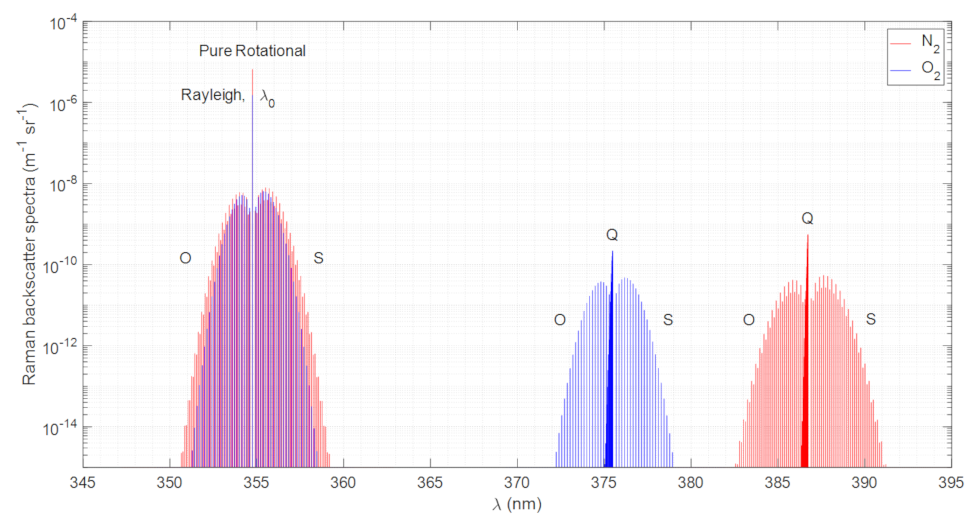
2.1. Pure Rotational and Vibro-Rotational Raman Spectra Calculation for N2 and O2

The result of energy interaction between an electromagnetic field and an atomic system is characterized by elastic and inelastic (Raman being one of them) processes. In the case of the Raman process, the scattered radiation is accompanied of an energy loss (Stokes wing of the Raman spectrum) or gain (anti-Stokes wing of the Raman spectrum). These changes, which can be observed as a frequency shift of the scattered photons, are directly related to the vibrational and rotational quantized energy states of the atomic system or molecule [14]. The vibrational-rotational Raman spectrum is defined by a distribution of spectral lines centered on a Q branch that possesses the highest intensity and two side branches: O and S, occurring at lower (Anti-stokes) and higher (Stokes) wavelengths, respectively. The final distribution of the vibrational-rotational Raman lines depends strictly on temperature T and excitation wave number ν0 = 1/λ0 [15].
A complete analysis of the Differential Backscatter Cross-Sections (DBCS) calculation for both PRR & VRR contributions from N2 and O2 is shown in Appendix A of this work.
The total contributions of the Raman backscatter spectra are estimated by the summation of the lines of the molecule’s spectral branches: O, Q & S (VRR) and O & S (PRR) weighted by their respective atmospheric concentration: 0.7808 for N2 and 0.2095 for O2 [14,16,17].
The lidar system used in this work employs a Nd:YAG (Neodymium-doped Yttrium Aluminum Garnet; Nd:Y3Al5O12) laser with a fundamental wavelength at 1064.28 nm. The second and third harmonics are thus expected at 532.14 nm and 354.76 nm, respectively [18]. Considering the third-harmonic excitation wavelength, λ0, of 354.76 nm and a temperature of 300 K, the computed Raman backscatter spectra for the PRR and the VRR contributions of N2 and O2, according to the Appendix A formulas, is shown in Figure 1 for 300 K temperature and standard sea-level pressure. The total contribution of the resulting intensities, calculated by the summation of the spectral lines for the PRR (O & S branches) and the VRR (O, Q & S branches) spectra, are given in Table 1. The ratio between PRR and VRR intensities from the backscatter spectra, PRR/VRR is 21.21 and 37.03 for N2 and O2, respectively.
In practice one cannot take advantage of the whole PRR spectrum because it encompasses the elastics return. Moreover, the selection of lines to pass through the interference filter must be such that sum of their DBCS is, to the maximum possible extent, insensitive to the temperature. Nevertheless, the overall cross section of that selection of N2 and O2 PRR spectrum lines still outweighs that of the total VRR spectrum.

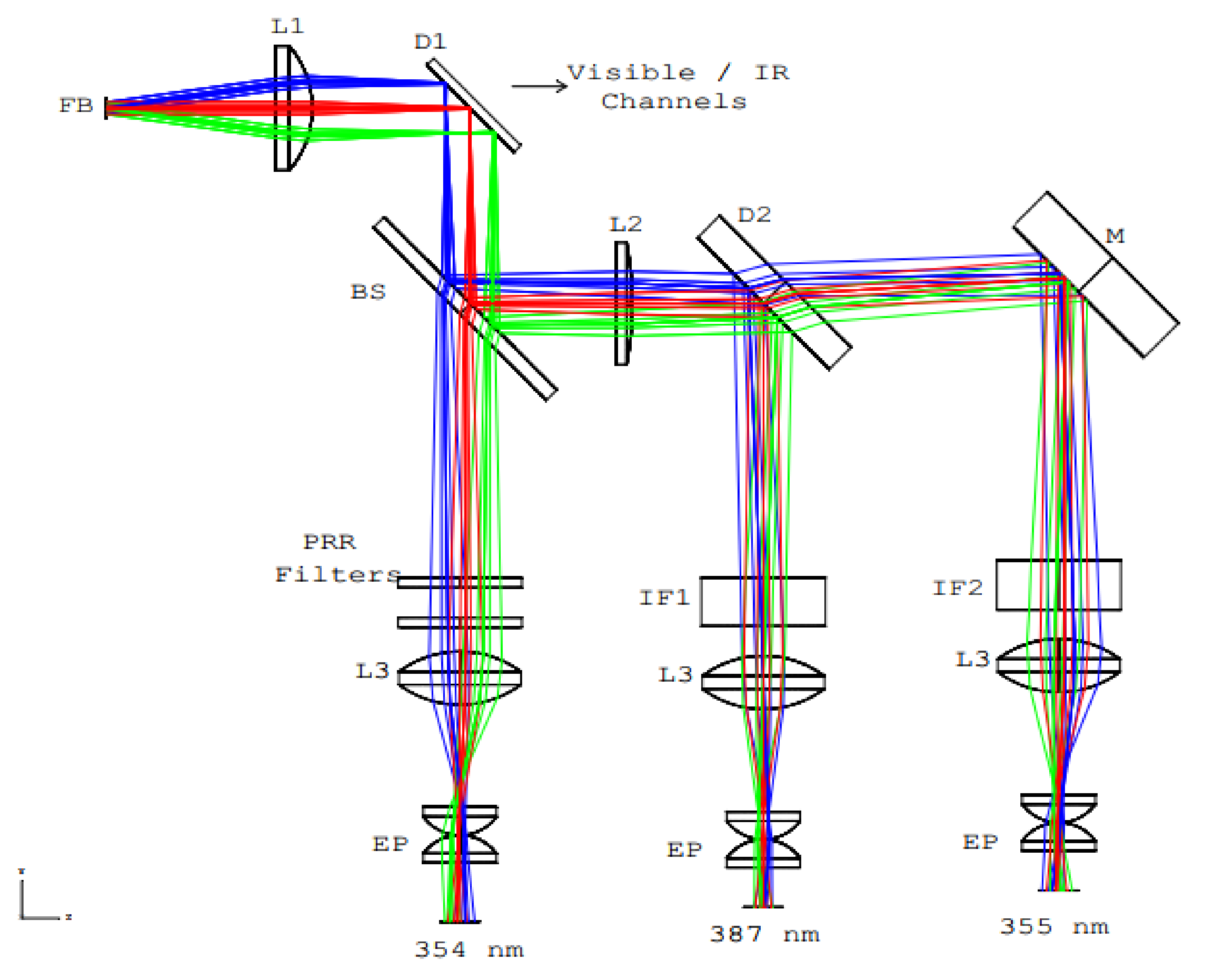
2.2. Optical Design and PRR Spectral Filtering

The EARLINET/UPC multi-wavelength lidar system was designed with a six channel wavelength-selection subsystem for the detection of Ultraviolet (UV), visible and Infrared (IR) backscatter returns [12,13]. The light collected by the telescope is transported by an optical fiber bundle (designed as FB in Figure 2) to the wavelength-selection subsystem. The optical setup of the UV branch has been especially redesigned for this study as shown in Figure 2. The main characteristics of the used optical elements are given in Table 2. Note that no attempt has been made to optimize the power reaching the Raman channels (e.g., by using a dichroic beam splitter, instead of the plain beam splitter labelled (BS) in Figure 2), because we were relying on a previous existing setup [12].
Using a first dichroic beam splitter (D1) UV and Visible-IR branches of the collected backscattered radiation are divided. After the first reflection on D1, the UV portion of the spectrum is divided into three channels. The first 50/50 beam splitter (BS) divides the incoming light into equal portions. Lens L2 corrects the divergence of the rays for the channels at 354.76 and 386.7 nm (N2 VRR spectra center wavelength). D2 reflects high UV wavelengths of the incoming radiation, redirecting this portion of the spectra to the 386.7 nm channel, and transmits the low UV wavelengths, which is reflected by a mirror (M) to the 355-nm channel. Lenses L3 and eye-pieces (EP) are used to, respectively, collimate and equally spread the radiation on the surface of the photomultiplier tube (PMT) detectors.
Elastic and VRR signals are optically filtered by, respectively, 1-nm and 3-nm bandwidth interference filters (see Table 2). As N2 atmospheric concentration is larger than O2, its total differential cross section is also larger (see Table 1). For this reason, the vibro-rotational channel is set to that of nitrogen. For the pure rotational contribution, two interference filters set in cascade are also used to minimize the crosstalk from the elastic channel. Between both O and S branches, only the anti-Stokes branch (O-branch) is considered to avoid aerosol fluorescence effects. Also, due to the technological impediments that hinder the effective elastic return rejection. For the fabrication of the PRR filters, a special request was sent to the manufacturer (Alluxa, North Laughlin Rd., Santa Rosa, CA 95403, USA) for two extremely narrow and steep interference filters with Center Wavelength (CWL) at 353.9 nm, bandwidth <1 nm, transmission at peak >60% and Optical Density (OD) of 4 (OD4) at 354.7 nm. The company delivered two filters with CWL at 353.9 nm, bandwidth <0.8 nm, transmission at peak >80% and OD4 at 354.7 nm. An effective suppression of the elastic wavelength is achieved by cascading these two interference filters although no attempt has been made to compare the response of the two cascaded filters to that of a single one. The resulting equivalent transmittance, assuming the response of the two-filter cascade is the product of the individual responses, is shown in Figure 3a, while the transmittance of the VRR filter is shown in Figure 3b. The corresponding differential backscatter cross-section are also overlapped on these figures.

2.3. PRR vs. VRR Channel Numerical Comparison

This sub-section is devoted to the estimation of the overall gain ratio between PRR and VRR channels i.e., Γ = PRR/VRR, particularized for the used system. Γ, can be defined as:
Γ = E C D S P R R E D C S V R R O P L P R R O P L V R R Γ P M T
where EDCS is the effective differential cross section, OPL is the optical path loss (excluding the interference filters) and ΓPMT is the gain ratio of the PMTs.
The EDCS is calculated by the summation of all the molecular differential cross-section lines σiPRR,VRR(J,T) (see Appendix A) of N2 and O2, in the case of the PRR spectrum, and N2 for the VRR spectrum, weighted by the respective atmospheric concentration Ni (0.7808 for N2 and 0.2095 for O2) and the filter transmittance ξ(λi,j):
E D C S P R R , V R R T = i j N i σ P R R , V R R i J , T ξ λ i , j
Subindexes i = 1, 2 correspond to the molecules N2 or O2, J stands for the rotational quantum number.
The estimated EDCS for the PRR and the VRR channels are given in Table 3. The resulting EDCSPRR/EDCSVRR ratio is 8.2.
The optical transmittance budget for PRR and VRR channels is also estimated in Table 3. All the optical elements situated on the optical path from the output of the fiber bundle to the PMT detectors are considered, except for the interference filters, which are already considered in the calculation of EDCS. The total OPL is 36% and 32% for PRR and VRR, respectively. These two values are very similar and indicate that both channels suffer similar optical losses along their respective optical path. With these numbers one can calculate the ratio (EDCSPRR/EDCSVRR) (OPLPRR/OPLVRR) which is equal to 9.2.
Finally, to consider a possible gain difference between the detectors, measurements with each PMT in its nominal position and with the PMTs swapped were made. In nominal conditions, PMT1 and PMT2 are the PMTs of the PRR and VRR channels, respectively. In the first measurement (nominal), PMT1 detected the signal of the PRR channel and PMT2 of the VRR one. In the second measurement (permuted), PMT2 detected the signal of the PRR channel and PMT1 of the VRR one. The background-subtracted lidar signals are shown in Figure 4. For the same channel, PMT1 gives a higher signal than PMT2 and thus has a higher gain. The PMT gain ratio, ΓPMT, was calculated by dividing the signals PMT1 over PMT2 averaged in the range [120, 700 m] for both PRR and VRR channels and taking the mean value of both ratios. We find ΓPMT = 1.32.
We can now calculate the overall gain ratio between PRR and VRR channels due to differences in interference filter transmittances, optical path losses and PMT gains [Equation (1)] being Γ = 12.14. This ratio not only estimates the total contribution of the EDCS of the PRR and VRR signals, but also contains experimental setup parameters (optics and detector gains), it is considered in the following a reference gain ratio to which real atmospheric signals can be compared to.

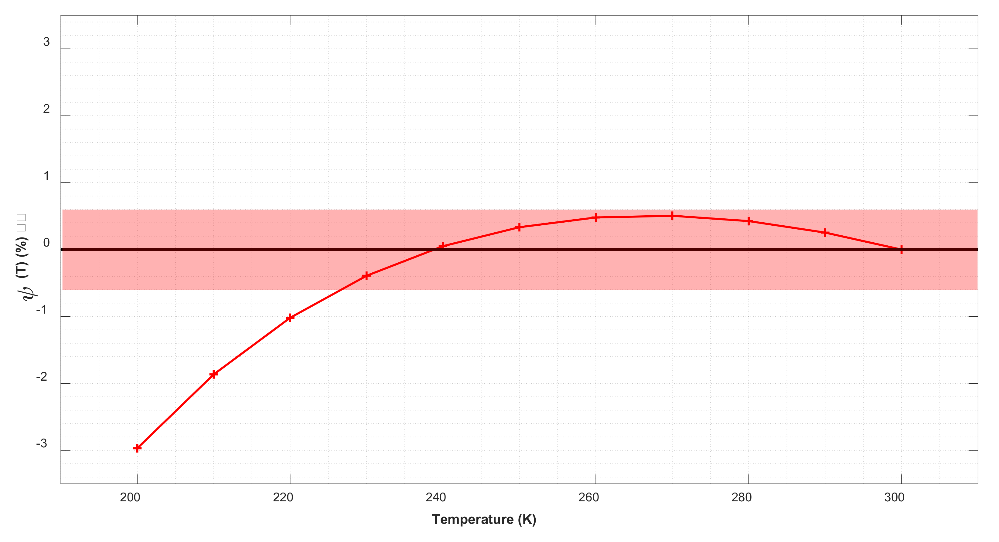
2.4. Temperature Analysis of the Effective Differential Cross-Section (PRR)

Pure rotational Raman lidars are commonly used for atmospheric temperature sensing since lines in the rotational spectra are sensitive to temperature [8]. This sub-section is devoted to the estimation of the temperature dependence of the PRR EDCS to verify that it can be neglected.
We computed EDCSPRR(T) [Equation (2)] variation in a conservative range of temperatures from 200 to 300 K. According to the US Standard atmosphere [19], 300 K corresponds to ground level and 200 K is reached at altitudes higher than 10 km. Considering T0 = 300 K as a reference, the relative variation of EDCSPRR(T) due to temperature has been estimated by analyzing the ratio:
ψ T = E D C S P R R T E D C S P R R T 0 E D C S P R R T
The results, shown in Figure 5, demonstrate that the relative variation of EDCSPRR(T) due to temperature does not exceed 3% in the 300 K–200 K temperature range and are even smaller than 0.5% for 230 < T < 300 K, i.e., below 10 km altitude.
To quantify the temperature-induced variations for the estimation of backscatter and extinction coefficients, we rely on the theory developed in [20] and afterwards employed for pure rotational Raman lidar applications by [7,11]. In these works, expressions for the calculation of backscatter and extinction coefficients are developed considering the temperature dependency:
β a e r z = β m o l + β m o l z 0 P λ R z 0 P λ 0 z N z P λ 0 z 0 P λ R z N z 0 σ e f f z σ e f f z 0
α a e r z = 1 2 d d z ln N z P λ R z z 2 + 1 2 d d z ln σ e f f z α m o l z
Subscripts aer and mol stand for aerosol and molecular contributions, λ0 and λR are excitation and Raman wavelengths respectively, and N is the molecular density. σeff (z) is the temperature-varying EDCSPRR as a function of height.
Temperature-induced variation for the backscatter coefficient can be estimated by computing the temperature height variation of σeff (z)/σeff (z0) (henceforth identified as Xβ) in Equation (4), reference height z0 was chosen to be 0 km. Temperature-induced error for the extinction coefficient was computed by the temperature height variation of the term (½)(d/dz)ln[σeff (z)] (henceforth identified as Δα) in Equation (5). For both calculations the temperature range was 288.15 to 223.25 K corresponding to a height range of 0 to 10 km according to the U.S. Standard Atmosphere model [19]. Results are shown in Figure 6. These computations show a temperature-induced variation for Xβ that does not exceed 1%. For the extinction, the absolute error variation is less than 1 Mm−1.
The authors in [7] performed a similar analysis for ψ(T) having found less than 1% of temperature dependency for the EDCS (λ0 = 532 nm). They reported a temperature-induced variation for the backscatter coefficient less than 1% and for the aerosol extinction coefficient error less than 2 Mm−1. In reference [11] (λ0 = 354.75 nm), the authors report a temperature variation for the backscatter coefficient was less than 4%. The extinction coefficient error is reported with an always negative variation of up to −1.6 Mm−1. Reference [21], λ0 = 1064 nm, reports a 4% of temperature dependence of the EDCS. All these results are shown in Table 4. Extinction relative errors were estimated for an aerosol load of 100 Mm−1 in all the references. This temperature analysis and comparative allows us to neglect changes related to the temperature influence in the PRR backscattered signal.

3. Results

Two nighttime and one daytime measurements are analyzed in this work. The day and time they were performed are indicated in Table 5, as well as some atmospheric parameters taken from Aerosol Robotic Network (AERONET) data, such as the aerosol optical depth at 440 nm, AOD440, and the Ångström exponent calculated from the wavelength pair (440 nm, 675 nm), AE440–675. The first nighttime measurement (N1) lasted for 3 h. The second nighttime study case (N2) corresponds to the first hour from N1. This 1-h-averaged measurement was chosen to examine the effect of temporal resolution on the quality of the retrievals. The daytime measurement (D1) lasted for 3 h as well. In N1 and N2 aerosols were of local origin and accumulated mostly in the planetary boundary layer (PBL): AOD440 is equal to 0.15 and AE440–675 to 1.27. In D1 most of the locally originated aerosols are in the PBL; mineral dust particles are present in the free troposphere up to 4.5–5 km. This situation is associated with a higher AOD440 (0.26) and a low AE440–675 (0.71).

3.1. PRR vs. VRR: Signal and Signal-to-Noise Ratio Comparisons

To get a quantitative comparison between PRR and VRR preprocessed (glued) signals, Signal-to-noise ratio (SNR) was calculated computing estimators of the mean value μ and the standard deviation σ over a 9-samples continuous sliding interval of the signal. SNR is estimated as μ/σ. To smooth the SNR calculation, a model was fitted to the σ estimator [22,23]. In photon-induced current devices, e.g., photomultiplier tubes, SNR can be calculated as [24]:
S N R = P s P q P s + P q P b + N E P 2 B
where Ps is the signal power, Pb is the background radiation, Pq is the quantum noise power defined as: Pq = 2FhcB/ηλ, B is the photoreceiver electrical bandwidth, and NEP is the noise equivalent power of the receiver. Values of the mean and the standard deviation estimators are related as μ = Ps and σ = (PqPs + PqPb + NEP2B)1/2, respectively.
The standard deviation σ, can be expressed as: σ = (K1μ + K2)1/2 with K1 = Pq and K2 = PqPb + NEP2B. To suppress the contribution of high varying near ranges, which could “fool” the overall fit, a logarithmic fitting is considered: log(σ) = ½log(K1μ + K2). The fitting was based on a nonlinear least-squares method [25,26] that retrieves the Ki coefficients that best fit the function ½log(K1μ + K2) to the estimator σ starting from first guess values of K1 and K2 and the previous estimated values of μ and log(σ). SNR was then re-calculated with the fitted σ.
Figure 7 shows the SNR estimated for the glued signals in a 0.5 to 5 km range. First 500 m were omitted to avoid overlap effects. For all three study cases, SNR for the PRR contribution (henceforth called SNRPRR) plotted in continuous lines, are higher than the respective SNR from the VRR (SNRVRR), plotted in dotted lines. For nighttime cases the enhancement factor, which essentially is the ratio between SNRPRR and SNRVRR, is quite constant for all the range, being 2.8 for N1 case and 2.6 for N2. Daytime case SNRPRR is quite constant for most of the interval. SNRVRR calculation kept variations despite the fitting process for the estimation of σ. Nevertheless, the enhancement factor of SNRPRR over SNRVRR signal is about 7.6 for most of the range. It is important to note that background radiation for the VRR channel (approximately 3-nm wide filter) is about three times larger than for the PRR channel (approximately 1-nm wide filter), which offers an added advantage in terms of SNR in daytime operation.
To verify the reliability of the calculation for these enhancement factors, estimated with the fitted model for σ, this section focusses on the comparison between SNR estimation against real signals gain. For nighttime conditions, background radiation Pb, as well as the noise equivalent power NEP, can be neglected from Equation (6). Therefore, SNR estimation may be expressed as:
S N R = μ P q μ = μ P q
The enhancement factor may be calculated as: SNRPRR/SNRVRR = {(μPRR/μVRR) × (PqVRR/PqPRR)}1/2. Considering that detectors from both channels are almost the same, the second term may be neglected. Therefore, the enhancement factor is proportional to the square root of the averaged signals ratio as SNRPRR/SNRVRR = (μPRR/μVRR)1/2. In a 1 to 3 km interval the computed square root of the averaged signal ratios is 2.54 and 2.53 for both N1 and N2 cases. These values work in accordance with the previously estimated enhancement factors of 2.8 and 2.6, differing less than 10% and 5% respectively.
For the daytime case, background radiation contribution predominates over NEP and Pq terms, resulting in a SNR estimation expressed as:
S N R = μ P q P b
The enhancement factor SNRPRR/SNRVRR, is recalculated as: SNRPRR/SNRVRR = (μPRR/μVRR)∙{(PqVRR/PqPRR)∙(PbVRR/PbPRR)}1/2 which essentially is proportional to the averaged signals ratio weighted by the squared root of the quantum noise power and the background radiation ratio for both PRR and VRR contributions. In the 1 to 3 km interval, the computed averaged signals ratio is 8.24. Omitting the fact that the second term is still affecting the relation, the resulting estimation differs less than 10% compared to the fitted enhancement factor (7.6).
Previously, in Section 2.3, an overall reference gain ratio between PRR and VRR signals was estimated as Γ = PRR/VRR = 12.14 [Equation (1)]. To compare the experimental data against this reference value it is necessary to consider the ratio between averaged signals: μPRR/μVRR, which stands for the realistic gain ratio between PRR and VRR detected signals. For nighttime cases, this ratio is about 6.45 and for daytime case is 8.24. Percentage differences between the experimental and theoretical value of this calculation reaches values of 47% (nighttime) and 32% (daytime). These differences may be explained by the lack of precision in the optical path losses which may be underestimated and also by possible changes of the aerosol load and the background radiation.

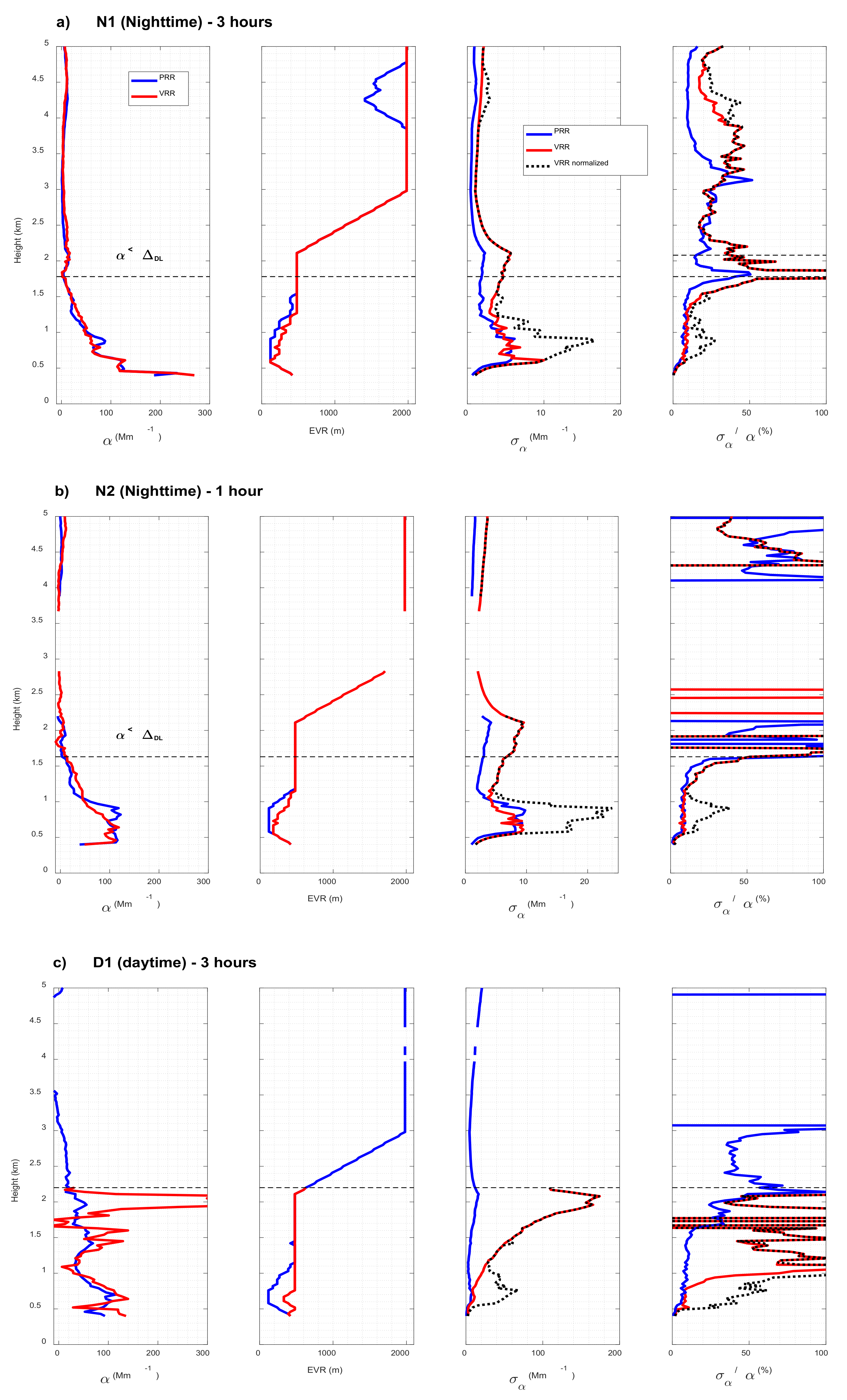
3.2. PRR vs. VRR: Optical Product Estimation and Comparison of Performances

The retrieval of the aerosol extinction and backscatter coefficients combining PRR and VRR signals with elastic signals has been performed by using the Single Calculus Chain (SCC) from the European Aerosol Research Lidar Network (EARLINET) [27,28,29]. It is the first time that the SCC is used to retrieve aerosol optical products from a combination of PRR and elastic signals. The optical processor module of the SCC is called EARLINET Lidar Data Analyzer (ELDA). ELDA was configured to retrieve backscatter and extinction coefficients at the same effective vertical resolution (product lidar ratio and extinction) using the Raman method [29]. This product also includes the effective vertical resolution, defined at each altitude point, calculated by ELDA to achieve the error goals fixed by the user [29]. As each Raman signal has its own statistical uncertainties the vertical resolution may differ from one measurement to the other. A coarser vertical resolution means that smoothing was more severe, and the retrieved products suffer loss of spatial information. Hence products with finer vertical resolution are more reliable. Only the product lidar ratio and extinction is shown in this work. VRR optical products for the EARLINET/UPC lidar system already exist in the SCC since 2011. VRR retrievals are restricted to only nighttime measurements. Daytime VRR retrievals have been tested in the past but either the SCC failed in performing the inversion or the results were not judged physically meaningful to be used for science purposes. Among many parameters needed in the SCC configuration, five are important for this work. For the VRR channel they are set as:
  • wavelengths set to 355 (elastic) and 387 nm (VRR),
  • extinction Ångström exponent is set to 1.0,
  • low and high range error thresholds are set to, respectively, 10 and 10% (nighttime) and 10 and 50% (daytime),
  • detection limits for the backscatter coefficient to 0.1 Mm−1 sr−1 and extinction to 5 Mm−1,
  • height range in which ELDA looks for a suitable calibration interval to 4–8 km.
The error threshold and the detection limit, noted respectively Δmax and ΔDL following [29] nomenclature, are thresholds used in the iterative procedure that calculates the vertical smoothing. In an initial step, the optical products are calculated with the maximum allowable vertical smoothing (500 m below 2 km and 2000 m above 2 km); in the following steps the vertical smoothing is reduced until the relative statistical uncertainty becomes larger than the user-defined error threshold or until the absolute uncertainty becomes larger than the user-defined detection limit (see [29] for more details). In daytime, ELDA was not able to successfully retrieve optical products with the VRR signals with a high-range (above 2 km) Δmax of 10%. So, this value was relaxed to 50% for daytime inversions.
For the PRR optical products, the same configuration as that of VRR products was used with the exceptions that wavelengths were set to 355 (elastic) and 354 nm (PRR). Low- and high range error thresholds, as well as detection limits, were kept unchanged. Finally, the statistical uncertainties associated to the optical products are estimated by Monte Carlo or error propagation methodologies [28,29].
To determine the region where most of the aerosols are, we used a simple threshold method on the extinction coefficient retrieved with the PRR signals. The limit to assume a small but non-negligible amount of aerosols was fixed to the detection limit, ΔDL, i.e., 5 Mm−1. On a monotonically decreasing profile of extinction coefficient, the region where αaer > ΔDL will represent the main surface aerosol layer. In the case of only one aerosol layer, the height at which the extinction coefficient reaches ΔDL should be a relatively good approximation of the PBL height [30].
Figure 8 shows for all three cases the vertical profiles of the aerosol backscatter coefficient, βaer, the aerosols extinction coefficient, αaer, the aerosol lidar ratio, i.e., the ratio αaeraer, noted LR, and the Effective Vertical Resolution (EVR), for both PRR and VRR retrievals. The time-height plot of the range-square corrected signal (in arbitrary units) is also reported to get an idea of the atmospheric structure. The subscript |PRR or |VRR behind a symbol indicates whether it was retrieved with the PRR or VRR signal, respectively. βaer and αaer with their associated uncertainties, as well as EVR are plotted as is without any post processing. Resulting negative values negative or larger than 100 sr are not represented in Figure 8.
In both nighttime cases, retrieved profiles of βaer and αaer from both pure rotational and vibro-rotational channels are quite similar. While the profiles of N1 are continuous, the retrievals of the 1-h nighttime case (N2) show discontinuities above the main surface aerosol layer related to negative extinction retrievals discarded in the output of the SCC. In case D1 the PRR retrieval is successful and that of the VRR is partly successful: αaer|VRR is retrieved but βaer|VRR is not (Figure 8c). It is worth recalling at this point that VRR retrievals with the EARLINET/UPC lidar system have always been restricted to nighttime conditions because the VRR inversion of daytime optical products either failed or was not judged physically meaningful to be used for science purposes. It is thus a small achievement that a profile of α|VRR was obtained for case D1. By looking at the profile of αaer|VRR, the explanation why βaer|VRR is not retrieved is quite straightforward: αaer|VRR is not retrieved above 2.2 km, i.e., EVR is not available in the range 4–8 km in which ELDA looks for a calibration interval for the calculation of βaer; in these conditions ELDA is not able to calculate the molecular backscatter coefficient βmol(z0) at the calibration height upon which depends the retrieval of βaer. In case D1, αaer|PRR and αaer|VRR agrees generally well up to 2.2 km. Differences are observed near the surface and in the last 500 m. Near the surface the difference is attributed to different vertical resolution, while between 1.7 and 2.2 km the difference is probably due to the degradation of the SNR in the VRR channel. Above 2.2 km αaer|VRR is not retrieved although aerosols are still present. αaer|PRR is retrieved above 2.2 km, although with increasing error bars and negative (i.e., non-physical) values starting above 3.1 km. The probable dust layer at 4–4.5 km is visible on the profile of βaer|PRR but not on that of αaer|PRR. This reveals the limit of the PRR performances in daytime conditions. Since optical products from PRR and VRR retrievals agree well, the quantitative, comparative analysis discussed in the next section is centered on their associated errors.
The profiles of LR can only be compared for both nighttime cases (βaer|VRR is not retrieved in case D1). Above the height at which αaer < ΔDL, the comparison is difficult because the low aerosol regime induces low signals and SNR, forcing ELDA to use full vertical resolution (2 km) in most of the upper interval. For that reason, the comparison is made only up to the height at which αaer < ΔDL, i.e., 1.78 and 1.63 km for N1 and N2, respectively. Up to those heights, the profiles of LR are very similar between both techniques. A difference can be pointed out in case N1: between 0.8 and 1.5 km LR|VRR variations appear smoother than the ones of LR|PRR. The explanation lies in two facts: in this height range, 1) the atmosphere is highly variable (see the time-height plot in Figure 8a) and 2) the vertical resolution of the PRR products is 20 to 40% smaller than that of the VRR products. Both facts yield a smoother profile of α|VRR, and thus of LR|VRR.
In all cases and at all altitude ranges the ratio EVR|PRR/EVR|VRR is smaller than or equal to 1, meaning that the extinction retrieval from PRR signals requires less or equal vertical smoothing than the VRR retrieval. In all cases also, below 2 km, EVR|VRR reaches its maximum value, 500 m, at lower heights than EVR|PRR. As seen in the plots of EVR in Figure 8, below 1.5 km, so typically in the PBL height in Barcelona [31], the lowest ratio EVR|PRR/EVR|VRR is 44, 36 and 25% for case N1, N2 and D1, respectively. Faced to VRR performances, PRR ones seem enhanced in daytime conditions (lower EVR|PRR/EVR|VRR ratio) and seem to decrease with increasing temporal resolution (EVR|PRR/EVR|VRR ratio higher for N1 than for N2).

4. Discussion

As a quantitative hint of the quality of the measurement the absolute and relative uncertainties were calculated for αaer and βaer. As it was mentioned before, ELDA estimates statistical uncertainties via the standard formula of statistical error propagation [28].
The statistical uncertainty of a product Xaer or βaer) is noted σX. The relative uncertainty is computed as σX/X. A low relative uncertainty (~10%) is an indicator of a reasonably good estimation [32]. The only Raman product that depends only on the Raman channel signal is the extinction coefficient. For comparison purposes it is the product chosen in Figure 9 and Figure 10. Figure 9 shows the profiles of αaer, EVR, σαaer and σαaeraer retrieved from both PRR and VRR signals. Since σαaer and σαaeraer for PRR and VRR channels were not calculated with the same vertical resolution, they are not directly comparable. To solve this issue, we have estimated the σαaer|VRR that ELDA would have calculated if the vertical resolution had been that of PRR.
To do so, we use the property that the standard deviation of the estimation of a slope (the method employed by the Raman algorithm) through a linear fit regression is inversely proportional to (N(N2 − 1))1/2, being N the number of samples used in the estimation and assuming that the noise is statistically the same in all samples [33]. For large values of N, such that N2»1, this standard deviation is proportional to N(N)1/2 = N3/2. With the native range resolution of the EARLINET/UPC lidar system of 3.75 m, typical EVR calculated by the SCC in the range 100–2000 m are obtained by averaging over a number of 26 to 534 samples. This number can be considered large, hence equivalent VRR σαaer and σαaeraer can be calculated at EVR|PRR by multiplying the original profiles by the profile of (EVR|VRR/EVR|PRR)3/2.
The recalculated or normalized profile is labelled “VRR normalized” in the legend of Figure 9. Figure 10 shows histograms with layer-mean values of EVR, σαaer and σαaeraer of both PRR and VRR retrievals in the main surface aerosol layer (αaer> ΔDL). In case D1 the layer-mean value was calculated between the ground and 2.2 km, which is the maximum height up to which α|VRR is defined. For comparison purposes, the layer-mean values of σα and σα/α of the VRR retrievals in Figure 10 are averages of the normalized magnitudes. For each magnitude (EVR, σαaer and σαaeraer) a reduction factor is obtained dividing the PRR retrieval by the VRR one.
In the following discussion (Figure 9 and Figure 10) the VRR retrievals of σαaer and σαaeraer are the normalized ones, i.e., the ones recalculated at EVR|PRR. In all cases and at all height ranges, the absolute uncertainty σαaer|PRR is smaller than the normalized σαaer|VRR (Figure 9). In the first few hundred meters near the surface, σαaer|PRR and the normalized σαaer|VRR are similar for all cases, but they start rapidly to differ and the difference between them increases with increasing height (especially in case D1). In both nighttime cases, above the first few hundred meters, the normalized σαaer|VRR is larger than σαaer|PRR but both profiles have a similar shape and no significant degradation of one compared to the other is observed up to the free troposphere. Contrarily, in case D1, the normalized σαaer|VRR increases strongly above 1.2 km up to values larger than 100 Mm−1, whereas σαaer|PRR stays below 15 Mm−1. This degradation of the statistical error of σαaer|VRR is related to the degradation of the SNR in the VRR channel mentioned in the former section and affects the quality of the retrieval already at 1.2 km within the main surface aerosol layer.
The relative uncertainty σαaeraer is also generally smaller for the PRR retrieval than for the normalized VRR one (Figure 9), although they can also exhibit similar values (e.g., range 2.4–3.2 km in case N1). In cases N1 and N2, below 1.5 km, σαaeraer for the PRR (and normalized VRR) retrievals are roughly constant and equal to 7 (14) and 8% (17)%, respectively. Above 1.5 km the relative uncertainty increases for both retrievals.
More variations are observed on the VRR retrieval. In case D1, below 1.5 km, σαaeraer for the PRR is relatively constant and stays below the quite reasonable value of 10%. This is a promising result for future daytime PRR retrievals. Above 1.5 km, σαaeraer increases to values of 30–40%. The normalized VRR σαaeraer increases quickly (from the very bottom of the profile) and very strongly (σαaeraer > 60% at 0.9 km) and features abrupt fluctuations, sometimes well above 100%.
We now examine the layer-mean values of EVR, of σαaer and σαaeraer in the main surface aerosol layer (αaer > ΔDL). We observe a small degradation of EVR between 3 h (N1) and 1 h (N2) temporal resolution (Figure 10a): EVR|PRR increases 7% and EVR|VRR 4% from N1 to N2. This non-linear degradation of both techniques makes PRR retrievals more effective for long time resolution (EVR|PRR/EVR|VRR is 0.83 for N2) than for shorter time resolution (EVR|PRR/EVR|VRR is 0.85 for N2). The most important EVR reduction occurs for the daytime case. The absolute (relative) uncertainty for the PRR retrieval is quite acceptable: 3.1 (9.3), 4.5 (11.0) and 6.3 (13.2%) Mm−1 for N1, N2 and D1, respectively. The normalized VRR σαaer is more than double for cases N1 and N2, and much larger for D1 (Figure 10b).
The corresponding σαaeraer are 24.2, 19.3 and 94.0% (Figure 10c), respectively. We conclude that the relative uncertainty of the PRR retrieval for 3-h nighttime measurements is roughly three times smaller than the VRR one. For 3-h daytime measurements it is roughly seven times smaller than the VRR one. Again, the highest reduction occurs for the daytime case.
Several attempts to retrieve aerosol extinction and backscatter via PRR implementations have been made in the recent past. As part of the discussion we aim to compare our results with some recent bibliographic endeavors, some of which have already been used for comparison in the temperature analysis Section 2.4. This section is focused on the measurements and the products obtained by [11] at 355 nm, [7] at 532 nm and [21] at 1064 nm.
The recent work of [11] is the most similar to ours, achieving aerosol extinction and backscatter retrievals with a PRR channel at 355nm. Both daytime and nighttime measurements were made with 1-h and 1-min. temporal resolutions, respectively. For nighttime study cases they were able to retrieve aerosol extinction in a 1.4–3.5 km range (main aerosol layer).
1-min time resolution profiles are compared to a 30-min integrated profile, finding variations of less than the 30% between products. For daytime study cases, extinction and backscatter were retrieved between 1.4 and a top height varying between 2.5 and 3.0 km. The only significant uncertainty considered is due to temperature, which has been compared in Section 2.4. The main differences of our work with respect to [11] are temporal resolutions. For our daytime study case, three hours temporal resolution permitted to retrieve aerosol extinction in a wider range, from 0.35 to 4 km. For nighttime study cases we could not reduce the temporal resolution below 1 h. Nevertheless, considering the reported variability between 1-min. and the averaged 30 min. profiles, we can infer that 1-h profiles can give a quite accurate glimpse of the overall aerosol load in a regular measurement.

5. Conclusions

A pure rotational Raman channel at 353.9 nm has been implemented in the EARLINET/UPC multi-wavelength lidar system. This new channel detects backscattered signals produced by the PRR effect of atmospheric N2 and O2 excited by the emission wavelength of 354.7 nm. Spectral filtering was obtained by cascading two extremely narrow and steep interference filters with an equivalent (i.e., for the two filters in cascade) CWL at 353.9 nm, FWHM < 0.8 nm, transmission at peak > 70% and OD8 at 354.7 nm. To study the temperature dependency, the sum of N2 and O2 differential backscatter cross section weighted by the respective atmospheric concentration and the filter transmittance was calculated as a function of temperature in a range 200–300 K. Variations were smaller than 3% in that range and smaller than 0.5% in the range 230–300 K corresponding to a height range of 0–10 km.
PRR and elastic signals have been inverted for the first time with the EARLINET Single Calculus Chain and profiles of aerosol extinction and backscatter coefficients have been retrieved successfully in daytime and nighttime conditions. To fully quantify the improvement of pure rotational over vibro-rotational Raman signals, simultaneous measurements at the VRR wavelength of 386.7 nm were performed. Two cases were taken with different aerosol loads and vertical structures. The signal-to-noise ratio was found in agreement with the theory: an increase of a factor 2.8 and ~7.6 was observed for 3-h nighttime and daytime measurements, respectively, when using PRR vs. VRR. Improvements in terms of retrieved optical properties are measured in terms of the reduction of the effective vertical resolution, EVR, and of the uncertainties (absolute, σαaer, and relative, σαaeraer) associated to the extinction coefficient in the main aerosol surface layer when using PRR retrievals vs. VRR ones.
For long (3 h), nighttime measurements EVR is reduced by 17%, σαaer is divided by 2 and and σαaeraer is divided by 3 when using PRR instead of VRR. During daytime and also 3-h measurements EVR is reduced by 20%, σαaer is divided by 10 and σαaeraer by 7 when using PRR instead of VRR. In the daytime case, the VRR extinction coefficient is retrieved in a limited height range (<2.2 km). This prevents the SCC from finding a suitable calibration range in the search height range of 4–8 km for the retrieval of the backscatter coefficient, so the advantage of using PRR instead of VRR is particularly evident in daytime conditions. For short (1 h), nighttime measurements EVR is reduced by 15%, σαaer is divided by a little more than 2 and σαaeraer is divided by a little less than 2 when using PRR instead of VRR.

Author Contributions

Conceptualization, M.S. and A.C.; methodology, M.S.; software, J.A.Z.-H. and G.D.; validation, J.A.Z.-H., A.R.-G. and M.S.; formal analysis, J.A.Z.-H.; investigation, J.A.Z.-H. and M.S.; resources, M.S.; data curation, J.A.Z.-H., A.R.-G. and C.M.-P.; writing—original draft preparation, J.A.Z.-H., M.S.; writing—review and editing, J.A.Z.-H., A.R.-G. and C.M.-P.; visualization, A.C.; supervision, M.S.; project administration, M.S.; funding acquisition, M.S. and A.C. All authors have read and agreed to the published version of the manuscript.

Funding

The research leading to these results has received funding from the H2020 program from the European Union (grant agreement no. 654109, 778349, 871115), the Spanish Ministry of Science and Innovation (ref. PID2019-103886RB-I00), the Spanish Ministry of Economy, Industry and Competitiveness (ref. CGL2017-90884-REDT), and the Unit of Excellence Maria de Maeztu (ref. MDM-2016-0600) financed by the Spanish Agencia Estatal de Investigación (AEI).

Data Availability Statement

The data presented in this study are available on request from the corresponding author.

Acknowledgments

The authors thank Igor Veselovskii for his advice and encouragement in the implementation of the PRR channel. Author J. A. Zenteno-Hernández thanks CONACyT for the 2018-000068-02NACF-29418 scholarship.

Conflicts of Interest

The authors declare no conflict of interest.

Appendix A. Pure Rotational and Vibro-Rotational Raman Differential Backscattering Cross-Section of N2 and O2 Calculation

Selection rules for nitrogen (N2) and oxygen (O2), are Δν = 0, ±1 for the vibrational quantum number and ΔJ = 0,±2 for the rotational quantum number. The Differential Backscatter Cross Section (DBCS) at an excitation wave number ν0 = 1/λ0 and temperature T is:
σ i P R R , V R R J , T = 2 π 4 ν 0 Δ ν J i P R R , V R R 4 g N Φ i P R R , V R R J 2 I N + 1 2 ξ exp h c B 0 J J + 1 k T i = S , Q J = 0 , 1 , 2 , 3 , i = O J = 2 , 3 , 4 ,
Subindex i = 1, 2 correspond to the molecules N2 or O2. O, Q and S stand for the spectrum branches. ξ ≈ kT/2hcB0 is the partition function, h is Planck’s constant, k is Boltzmann constant and c is the speed of light.
Molecular constants are shown in Table A1, Table A2 and Table A3. Data compiled from [14,16,34,35,36,37].
Table A1. Statistical weigh factor gN and nuclear spins IN values for N2 and O2.
gNIN
N26 for J even; 3 for J odd1
O20 for J even; 1 for J odd0
Table A2. Ground-state rotational and centrifugal distortion constants.
B1
[m−1]
B0
[m−1]
D0
[m−1]
N2197.219198.9575.76 × 10−4
O2142.188143.7684.85 × 10−4
For the vibro-rotational contribution which is displaced an amount νvib from the excitation wavelength number ν0, the frequency shifts are given by:
Δ ν J V R R S ν v i b + 4 J + 6 B 1 , J = 0 , 1 , 2 ,
Δ ν J V R R Q ν v i b + J J + 1 B 1 B 0 J = 0 , 1 , 2 ,
Δ ν J V R R O ν v i b 4 J 2 B 0 , J = 2 , 3 , 4 ,
For each molecule, their specific vibrational wavenumber is νvib = 2330.7 cm−1 and νvib = 1556.4 cm−1 for N2 and O2, respectively. Phi functions are defined as:
Φ V R R S J = h 8 π 2 c ν v i b 1 exp h c ν v i b / k T 7 J + 1 J + 2 30 2 J + 3 γ 2 , J = 0 , 1 , 2 ,
Φ V R R Q J = h 2 J + 1 8 π 2 c ν v i b 1 exp h c ν v i b / k T α 2 + 7 J + 1 J + 2 45 2 J 1 2 J + 3 γ 2 , J = 0 , 1 , 2 ,
Φ V R R O J = h 8 π 2 c ν v i b 1 exp h c ν v i b / k T 7 J J 1 30 2 J 1 γ 2 , J = 2 , 3 , 4 ,
For the pure rotational contribution, a few considerations must be taken; as there is no excited vibrational state, both Stokes and Anti-Stokes branches spread around the excitation wavelength number ν0. Q branch corresponds to Rayleigh scattering which can be estimate as σQPRR (J,T) = QRayleigh = (2π)4ν04∙(a2 + (7γ2/180)) [14]. Also, the coefficient h{8π2cνvib∙[1 − exp(hcνvib/kT)]}−1 can be approximated to 1 [38]. Therefore, frequency shifts around the excitation wavelength are:
Δ ν J P R R S 4 J + 6 B 0 , J = 0 , 1 , 2 ,
Δ ν J P R R O 4 J 2 B 0 , J = 2 , 3 , 4 ,
Phi functions are defined as:
Φ P R R S J = 7 J + 1 J + 2 30 2 J + 3 γ 2 , J = 0 , 1 , 2 ,
Φ P R R O J = 7 J J + 1 30 2 J 1 γ 2 , J = 2 , 3 , 4 ,
Remaining constants are shown in Table A3.
Table A3. Molecular constants.
a2
[m6/(4πε0)2]
γ2
[m6/(4πε0)2]
a′2
[(4πε0)2 m2/kg]
γ′2
[(4πε0)2 m2/kg]
N23.17 × 10−600.52 × 10−602.62 × 10−144.23 × 10⁻¹⁴
O22.66 × 10-601.26 × 10−601.63 × 10−146.46 × 10⁻¹⁴
For LiDAR applications, the Raman Backscatter spectrum of N2 and O2 is calculated by weighting the DBCS by the atmospheric concentration N, of either N2 (0.7808) or O2 (0.2095) [16] as:
β R i = N σ P R R , V R R i J , T

References

  1. Comerón, A.; Muñoz-Porcar, C.; Rocadenbosch, F.; Rodríguez-Gómez, A.; Sicard, M. Current research in lidar technology used for the remote sensing of atmospheric aerosols. Sensors 2017, 17, 1450. [Google Scholar] [CrossRef] [Green Version]
  2. Ansmann, A.; Riebesell, M.; Weitkamp, C. Measurement of atmospheric aerosol extinction profiles with a Raman lidar. Opt. Lett. 1990, 15, 746. [Google Scholar] [CrossRef] [PubMed]
  3. Ansmann, A.; Riebesell, M.; Wandinger, U.; Weitkamp, C.; Voss, E.; Lahmann, W.; Michaelis, W. Combined raman elastic-backscatter LIDAR for vertical profiling of moisture, aerosol extinction, backscatter, and LIDAR ratio. Appl. Phys. B Photophys. Laser Chem. 1992, 55, 18–28. [Google Scholar] [CrossRef]
  4. Measures, R.M. Laser Remote Sensing Fundamentals and Applications; Reprint; Krieger Publisher Company: Malabar, FL, USA, 1992. [Google Scholar]
  5. Kovalev, V.A.; Eichinger, W.E. Elastic Lidar Theory, Práctice and Analysis Methods; John Wiley & Sons, Inc.: Hoboken, NJ, USA, 2004. [Google Scholar]
  6. Ansmann, A.; Müller, D. Lidar and Atmospheric Aerosol Particles. In Lidar. Range-Resolved Optical Remote Sensing of the Atmosphere; Weitkamp, C., Ed.; Springer Series in Optical Sciences; Springer: New York, NY, USA, 2005; Volume 102, pp. 105–141. ISBN 0-387-40075-3. [Google Scholar]
  7. Veselovskii, I.; Whiteman, D.N.; Korenskiy, M.; Suvorina, A.; Perez-Ramirez, D. Use of rotational Raman measurements in multiwavelength aerosol lidar for evaluation of particle backscattering and extinction. Atmos. Meas. Tech. 2015, 8, 4111–4122. [Google Scholar] [CrossRef] [Green Version]
  8. Behrendt, A.; Reichardt, J. Atmospheric temperature profiling in the presence of clouds with a pure rotational Raman lidar by use of an interference-filter-based polychromator. Appl. Opt. 2000, 39, 1372. [Google Scholar] [CrossRef] [PubMed]
  9. Kim, D.; Cha, H. Rotational Raman lidar: Design and performance test of meteorological parameters (aerosol backscattering coefficients and temperature). J. Korean Phys. Soc. 2007, 51, 352–357. [Google Scholar] [CrossRef]
  10. Achtert, P.; Khaplanov, M.; Khosrawi, F.; Gumbel, J. Pure rotational-Raman channels of the Esrange lidar for temperature and particle extinction measurements in the troposphere and lower stratosphere. Atmos. Meas. Tech. 2013, 6, 91–98. [Google Scholar] [CrossRef] [Green Version]
  11. Ortiz-Amezcua, P.; Bedoya-Velásquez, A.E.; Benavent-Oltra, J.A.; Pérez-Ramírez, D.; Veselovskii, I.; Castro-Santiago, M.; Bravo-Aranda, J.A.; Guedes, A.; Guerrero-Rascado, J.L.; Alados-Arboledas, L. Implementation of UV rotational Raman channel to improve aerosol retrievals from multiwavelength lidar. Opt. Express 2020, 28, 8156–8168. [Google Scholar] [CrossRef]
  12. Kumar, D.; Rocadenbosch, F.; Sicard, M.; Comeron, A.; Muñoz, C.; Lange, D.; Tomás, S.; Gregorio, E. Six-channel polychromator design and implementation for the UPC elastic/Raman lidar. In Proceeding of the Lidar Technologies, Techniques, and Measurements for Atmospheric Remote Sensing VII, Prague, Czech Republic, 30 September 2011. [Google Scholar]
  13. Rodríguez-Gómez, A.; Sicard, M.; Granados-Muñoz, M.J.; Ben Chahed, E.; Muñoz-Porcar, C.; Barragán, R.; Comerón, A.; Rocadenbosch, F.; Vidal, E. An architecture providing depolarization ratio capability for a multi-wavelength raman lidar: Implementation and first measurements. Sensors 2017, 17, 2957. [Google Scholar] [CrossRef] [Green Version]
  14. Wandinger, U. Raman Lidar. In Lidar. Range-Resolved Optical Remote Sensing of the Atmosphere; Weitkamp, C., Ed.; Springer Series in Optical Sciences; Springer: New York, NY, USA, 2005; Volume 102, pp. 241–271. ISBN 0-387-40075-3. [Google Scholar]
  15. Liu, F.; Yi, F. Lidar-measured atmospheric N2 vibrational-rotational Raman spectra and consequent temperature retrieval. Opt. Express 2014, 22, 27833. [Google Scholar] [CrossRef]
  16. Behrendt, A. Temperature Measurements with Lidar. In Lidar. Range-Resolved Optical Remote Sensing of the Atmosphere; Weitkamp, C., Ed.; Springer Series in Optical Sciences; Springer: New York, NY, USA, 2005; Volume 102, pp. 273–305. ISBN 0-387-40075-3. [Google Scholar]
  17. Inaba, H.; Kobayasi, T. Laser-Raman radar -Laser-Raman scattering methods for remote detection and analysis of atmospheric pollution. Opto-Electronics 1972, 4, 101–123. [Google Scholar] [CrossRef]
  18. Verdeyen, J.T. Laser Electronics, 3rd ed.; Prentice Hall: Englewood Cliffs, NJ, USA, 1995. [Google Scholar]
  19. U.S. Standard Atmosphere, 1976; National Oceanic and Atmospheric Administration: Washington, DC, USA, 1976.
  20. Whiteman, D.N.I. Evaluating the temperature-dependent lidar equations. Appl. Opt. 2003, 42, 2571–2592. [Google Scholar] [CrossRef] [PubMed]
  21. Haarig, M.; Engelmann, R.; Ansmann, A.; Veselovskii, I.; Whiteman, D.N.; Althausen, D. 1064nm rotational Raman lidar for particle extinction and lidar-ratio profiling: Cirrus case study. Atmos. Meas. Tech. 2016, 9, 4269–4278. [Google Scholar] [CrossRef] [Green Version]
  22. Md Reba, M.N.; Rocadenbosch, F.; Sicard, M. A straightforward signal-to-noise ratio estimator for elastic/Raman lidar signals. Remote Sens. Clouds Atmos. XI 2006, 6362, 636223. [Google Scholar]
  23. Liu, Z.; Hunt, W.; Vaughan, M.; Hostetler, C.; McGill, M.; Powell, K.; Winker, D.; Hu, Y. Estimating random errors due to shot noise in backscatter lidar observations. Appl. Opt. 2006, 45, 4437–4447. [Google Scholar] [CrossRef]
  24. Agishev, R.R.; Comeron, A.; Gross, B.; Moshary, F.; Ahmed, S.; Gilerson, A.; Vlasov, V.A. Application of the method of decomposition of lidar signal-to-noise ratio to the assessment of laser instruments for gaseous pollution detection. Appl. Phys. B Lasers Opt. 2004, 79, 255–264. [Google Scholar] [CrossRef] [Green Version]
  25. Coleman, T.F.; Li, Y. An Interior Trust Region Approach for Nonlinear Minimization Subject to Bounds. SIAM J. Optim. 1996, 6, 418–445. [Google Scholar] [CrossRef] [Green Version]
  26. Coleman, T.F.; Li, Y. On the convergence of interior-reflective Newton methods for nonlinear minimization subject to bounds. Math. Program. 1994, 67, 189–224. [Google Scholar] [CrossRef]
  27. D’Amico, G.; Amodeo, A.; Baars, H.; Binietoglou, I.; Freudenthaler, V.; Mattis, I.; Wandinger, U.; Pappalardo, G. EARLINET Single Calculus Chain-overview on methodology and strategy. Atmos. Meas. Tech. 2015, 8, 4891–4916. [Google Scholar] [CrossRef] [Green Version]
  28. D’Amico, G.; Amodeo, A.; Mattis, I.; Freudenthaler, V.; Pappalardo, G. EARLINET Single Calculus Chain-Technical-Part 1: Pre-processing of raw lidar data. Atmos. Meas. Tech. 2016, 9, 491–507. [Google Scholar] [CrossRef] [Green Version]
  29. Mattis, I.; D’Amico, G.; Baars, H.; Amodeo, A.; Madonna, F.; Iarlori, M. EARLINET Single Calculus Chain-Technical-Part 2: Calculation of optical products. Atmos. Meas. Tech. 2016, 9, 3009–3029. [Google Scholar] [CrossRef] [Green Version]
  30. Melfi, S.H.; Spinhirne, J.D.; Chou, S.-H.; Palm, S.P. Lidar Observations of Vertically Organized Convection in the Planetary Boundary Layer over the Ocean. J. Clim. Appl. Meteorol. 1985, 24, 806–821. [Google Scholar] [CrossRef]
  31. Sicard, M.; Pérez, C.; Rocadenbosch, F.; Baldasano, J.M.; García-Vizcaino, D. Mixed-layer depth determination in the Barcelona coastal area from regular lidar measurements: Methods, results and limitations. Boundary-Layer Meteorol. 2006, 119, 135–157. [Google Scholar] [CrossRef] [Green Version]
  32. Taylor, J.R. An Introduction to Error Analysis: The Study of Uncertainties in Physical Measurements. Meas. Sci. Technol. 1998, 51, 57. [Google Scholar] [CrossRef] [Green Version]
  33. Goodman, L.A. On the Exact Variance of Products. J. Am. Stat. Assoc. 1960, 55, 708–713. [Google Scholar] [CrossRef]
  34. Murphy, W.F.; Holzer, W.; Bernstein, H.J. Gas Phase Raman Intensities: A Review of “Pre-Laser” Data. Appl. Spectrosc. 1969, 23, 211–218. [Google Scholar] [CrossRef]
  35. Alms, G.R.; Burnham, A.K.; Flygare, W.H. Measurement of the dispersion in polarizability anisotropies. J. Chem. Phys. 1975, 63, 3321–3326. [Google Scholar] [CrossRef]
  36. Buldakov, M.A.; Ippolitov, I.I.; Korolev, B.V.; Matrosov, I.I.; Cheglokov, A.E.; Cherepanov, V.N.; Makushkin, Y.S.; Ulenikov, O.N. Vibration rotation Raman spectroscopy of gas media. Spectrochim. Acta Part A Mol. Spectrosc. 1996, 52, 995–1007. [Google Scholar] [CrossRef]
  37. Long, D.A. The Raman Effect: A Unified Treatment of the Theory of Raman Scattering by Molecules; John Wiley & Sons Ltd.: Hoboken, NJ, USA, 2002; Volume 8, ISBN 0471490288. [Google Scholar]
  38. Inaba, H. Detection of atoms and molecules by Raman scattering and resonance fluorescence. In Laser Monitoring of the Atmosphere; Hinkley, E.D., Ed.; Springer: Berlin/Heidelberg, Germany, 1976; pp. 153–236. [Google Scholar]
Figure 1. Pure rotational and vibro-rotational Raman backscatter spectra intensities calculated for diatomic Nitrogen (N2) and diatomic Oxygen (O2). Excitation wavelength: 354.76 nm. The spectra shown correspond to a 300 K temperature and to a 1013 hPa pressure.
Sensors 21 01277 g001
Figure 2. Zemax optical layout. FB stands for fiber bundle, L for lens, D for dichroic mirror, BS for beam splitter, EP for eyepiece, IF for interferential filter and M for mirror. Blue/red/green rays have a divergence of 15°, 0° and −15°. 15° corresponds to the numerical aperture of the fiber bundle.
Sensors 21 01277 g002
Figure 3. (a) N2 and O2 pure rotational Raman spectra (left axis) and filter transmittance (right axis) (b) N2 vibro-rotational Raman spectrum (left axis) and filter transmittance (right axis). The spectra shown correspond to a 300 K temperature and to a 1013 hPa pressure.
Sensors 21 01277 g003
Figure 4. Raw lidar signal at the Photomultiplier tube (PMT) outputs over a 50 Ω load of PRR and VRR channels in nominal condition (PRR → PMT1; VRR → PMT2) and permuted (PRR → PMT2; VRR → PMT1). The background noise offset has been subtracted to the lidar signal.
Sensors 21 01277 g004
Figure 5. Relative temperature variation of ψ(T). Reference temperature T0 = 300 K. The shaded area indicates relative errors in the range [−0.5, 0.5].
Sensors 21 01277 g005
Figure 6. (a) Temperature-induced variation for the backscatter coefficient (b) temperature-induced error for the extinction coefficient. Temperature profile from U.S. Standard Atmosphere.
Sensors 21 01277 g006
Figure 7. PRR and VRR Signal-to-noise ratio.
Sensors 21 01277 g007
Figure 8. Aerosol backscatter and extinction coefficients, lidar ratio and effective vertical resolution retrieved by the Single Calculus Chain (SCC) from PRR and VRR signals for case (a) N1, (b) N2 and (c) D1. On the plot of the vertical resolution, the ratio of the resolutions PPR to VRR is reported (black line, top axis). Time-height plots of the range-square corrected signal (in arbitrary units) are reported in the far-right plot. In (a,b) the black horizontal dashed line represents the lowest height for which α < ΔDL. In (c) it represents the highest height for which α | VRR is retrieved. The legend in the first plot of Figure 8a applies to all plots.
Sensors 21 01277 g008
Figure 9. Aerosol extinction coefficient, vertical resolution, absolute and relative errors retrieved by the SCC from PRR and VRR signals for case (a) N1, (b) N2 and (c) D1. In (a,b) the black horizontal dashed lines represent the lowest height for which α < ΔDL. In (c) it represents the highest height for which α|VRR is retrieved. “VRR normalized” refers to the magnitude recalculated at or normalized to EVR|PRR. The legends in Figure 9a apply to all plots.
Sensors 21 01277 g009
Figure 10. Comparative histograms of layer-mean values of the (a) vertical resolution, (b) absolute uncertainty and (c) relative uncertainty in the main surface aerosol layer (αaer > ΔDL) retrieved by the SCC from PRR and VRR signals for cases N1, N2 and D1. Black plus signs (right axis) are the ratio PRR to VRR. For layer-mean values exceeding the selected vertical scale the numerical value is reported in black on the top of the bar.
Sensors 21 01277 g010
Table 1. Calculated intensities of the Raman backscatter spectra of Pure rotational Raman (PRR) and Vibro-rotational Raman (VRR) for diatomic nitrogen (N2) and diatomic oxygen (O2).
UnitsN2O2
PRR10−8 m−1 sr−112.44238.0672
VRR10−8 m−1 sr−10.58660.2178
Table 2. Description of the optical elements.
ElementAcronymManufacturer
Model
Description
LensL1Edmund Optics
T46-266/T08-058
UV GFS UV-AR coating, PCX D = 25.4 mm, BFL = 33.03 mm,
DichroicD1CVI
LWP-45-RU407/386/355-TU1064/607/532
Side 1: Ru ≥ 99% @407, 386, 355 nm and Tu ≥ 85% @1064, 607, 532 nm
LensL2Edmund Optics
T46-271/T08-007
UV GFS UV-AR coating, PCX D = 25.4 mm, BFL = 147.82 mm,
BeamsplitterBSMelles Griot
03BTQ027
UV GSFS beamsplitter D = 50 mm, Tr = 3 mm
DichroicD2CVI
SWP-45-RU407-TU355-PW-1525-UV
Side 1: Ru ≥ 98% @407 nm, Tu ≥ 60% @355 nm, Side 2: AR @ 355 nm
MirrorMMelles Griot
02MFG017
Protected aluminum round flat mirror D = 38 mm, T = 10 mm
PRR Interference filtersPRR FiltersAlluxa
Custom made
CWL: 353.9 nm, FWHM: 0.8 nm
VRR Interference filterIF1Barr
Custom made
CWL: 386.7 nm, FWHM: 3 nm
Elastic Interference filterIF2Barr
Custom made
CWL: 354.7 nm, FWHM: 1 nm
LensL3Edmund Optics
T46-292/T08-077
UV GSF UV-AR coating, DCX D = 25.4 mm, BFL = 21.34 mm, CT = 10.9 mm
EyepieceEPEdmund OpticsF = 18 mm, d = 15 mm
Table 3. Calculated Effective Differential Cross-Sections (EDCS) and Optical Path Loss (OPL) of Pure rotational Raman (PRR) and Vibro-rotational Raman (VRR) lines/channels. The optical path loss is estimated for the entire optical path behind the fiber bundle excluding the interference filters.
UnitsElementPRRVRR
EDCS10−8 m−1 sr−1-3.50650.4252
-(N2 and O2)(N2)
OPLFractionL10.90.9
D10.990.99
BS0.50.5
L2-0.9
D2-0.98
L30.90.9
EP0.90.9
OPL0.360.32
(EDCS)(OPL)10−8 m−1 sr−1-1.26230.1360
Table 4. Temperature dependence comparison with previous works. Temperature range: 230–300 K. Aerosol load of 100 Mm−1.
Veselovskii (2015)Haarig (2016)Ortiz (2020)This Work
λ0 = 532 nmλ0 = 1604 nmλ0 = 355 nmλ0 = 355 nm
ψ(T)<1 %<4%--<0.5%
Xβ<1 %--<4%<1%
Δα<2 Mm−1--<−1.6 Mm−1<1 Mm−1
Δα (%)<2%--<1.6%<1%
Table 5. Main characteristics of the measurements used in this work. The AERONET measurements are level 1.5.
CaseUnitsN1N2D1
Conditions NighttimeNighttimeDaytime
Date 11/3/202011/2/202021/3/2020
Start timeUT18:5718:5712:46
Temporal resolutionHours313
Nearest AERONET
TimeUT17:0517:0512:59
AOD440 0.150.150.26
AE440–675 1.271.270.71
Probable airmass origin LocalLocalLocal, dust in the FT
Publisher’s Note: MDPI stays neutral with regard to jurisdictional claims in published maps and institutional affiliations.

