
A Flexible Coding Scheme Based on Block Krylov Subspace Approximation for Light Field Displays with Stacked Multiplicative Layers


Department of Electrical Engineering, Indian Institute of Technology Madras, Chennai 600036, India
*
Author to whom correspondence should be addressed.
†
These authors contributed equally to this work.
Sensors 2021, 21(13), 4574; https://doi.org/10.3390/s21134574
Submission received: 22 March 2021
/
Revised: 13 June 2021
/
Accepted: 18 June 2021
/
Published: 4 July 2021
(This article belongs to the Collection Machine Learning for Multimedia Communications)
Abstract
:To create a realistic 3D perception on glasses-free displays, it is critical to support continuous motion parallax, greater depths of field, and wider fields of view. A new type of Layered or Tensor light field 3D display has attracted greater attention these days. Using only a few light-attenuating pixelized layers (e.g., LCD panels), it supports many views from different viewing directions that can be displayed simultaneously with a high resolution. This paper presents a novel flexible scheme for efficient layer-based representation and lossy compression of light fields on layered displays. The proposed scheme learns stacked multiplicative layers optimized using a convolutional neural network (CNN). The intrinsic redundancy in light field data is efficiently removed by analyzing the hidden low-rank structure of multiplicative layers on a Krylov subspace. Factorization derived from Block Krylov singular value decomposition (BK-SVD) exploits the spatial correlation in layer patterns for multiplicative layers with varying low ranks. Further, encoding with HEVC eliminates inter-frame and intra-frame redundancies in the low-rank approximated representation of layers and improves the compression efficiency. The scheme is flexible to realize multiple bitrates at the decoder by adjusting the ranks of BK-SVD representation and HEVC quantization. Thus, it would complement the generality and flexibility of a data-driven CNN-based method for coding with multiple bitrates within a single training framework for practical display applications. Extensive experiments demonstrate that the proposed coding scheme achieves substantial bitrate savings compared with pseudo-sequence-based light field compression approaches and state-of-the-art JPEG and HEVC coders.
1. Introduction
Realistic presentation of a three-dimensional world on displays has been a long-standing challenge for researchers in the areas of plenoptics, light field, and full parallax imaging [1,2,3]. Glasses-free or naked-eye autostereoscopic displays have replaced stereoscopic displays which offer motion parallax for different viewing directions [4]. However, current naked-eye displays fall far short of truly recreating continuous motion parallax, greater depth-of-field, and a wider field-of-view for visual reality [5,6,7,8].
Designs based on a single display panel attached with a parallax barrier or special lens (lenticular screen or integral photography lens) usually suffer from inherent resolution limitations. The resolution for each view decreases with an increase in multiple viewing directions. Thus, supporting a full parallax visualization of the 3D scene is impractical [4]. On the other hand, both monitor-style and large-scale systems based on several projectors introduce a wide viewing approach, but such light field displays do not maintain a thin form factor and require ample space for the entire setup. Besides, such large-scale systems require costly hardware and a computationally expensive light field processing pipeline to reproduce high-quality views [9,10].
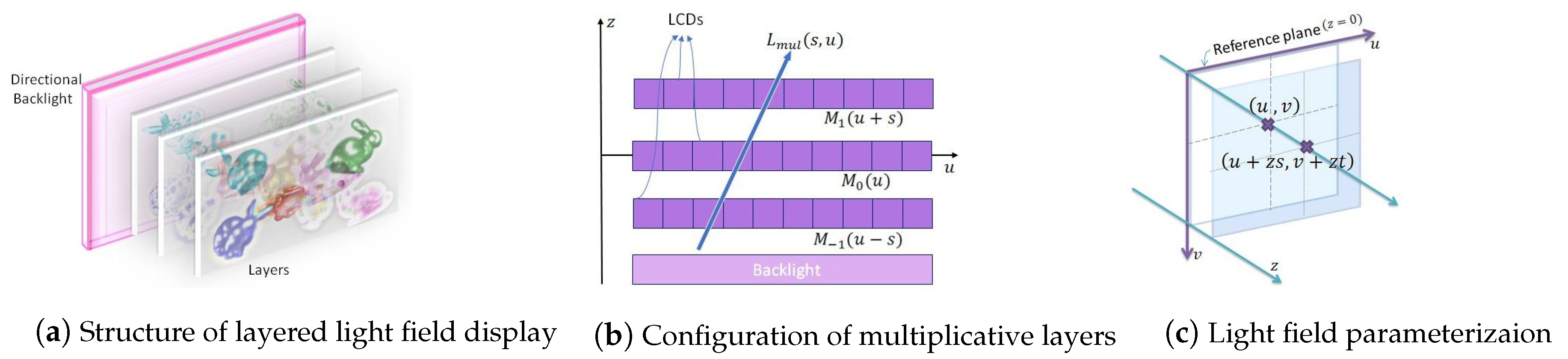
Multi-layered or tensor light field displays offer an optimized solution to support direction-dependent outputs simultaneously, without sacrificing the resolution in reproducing dense light fields. This is deemed as a critical characteristic of glasses-free multi-view displays [5,11,12,13,14,15,16,17]. A typical structure of a layered 3D display is demonstrated in Figure 1a. It is composed of a few light-attenuating pixelized layers stacked with small intervals in front of a backlight. The transmittance of pixels on each layer can be controlled independently by carrying out light-ray operations (multiplication and addition) on the layered patterns. A multi-layered display with liquid crystal display (LCD) panels and a backlight is implemented by performing multiplicative operations on layers, and additive layers are fabricated with holographic optical elements (HOEs) and projectors [14]. With this structure, the layer patterns allow light rays to pass through different combinations of pixels depending on the viewing directions. As shown in Figure 1b, multiplicative layer patterns overlap with different shifts in observed directions. With layered displays, we can precisely reproduce multi-view images or an entire light field simultaneously with high resolution by considering just a few light attenuating layers. Further, compactly representing the light field using transmittance patterns of only a few layers offers display adaptation. Directed from a target light field, transmittance patterns of stack pixelized layers are useful in determining the multi-view images required for various display types design with light fields, such as projection displays [9,18], mixed reality head-mounted displays [19,20,21], table-top displays, and mobile platforms [22]. It is critical to analyze the intrinsic redundancy in light fields to generate an efficient 3D production and content delivery pipeline using multi-layer-based approaches. This is essential to efficiently represent (multiplicative or additive) stacked layers for the desired light-field output.
In this paper, we address the problem of light field dimensionality reduction for existing multi-layer or tensor 3D displays. The CNN is employed to optimize multiplicative layers obtained from light field data. CNN-based methods are proven to be better in terms of balance between computation time and accuracy than the previous analytical optimization approaches based on non-negative tensor factorization [5,14,17,18]. A novel coding scheme for the multiplicative layers is proposed based on a randomized block Krylov singular value decomposition framework. The proposed algebraic representation of stacked multiplicative layers on the Krylov subspace approximates the hidden low-rank structure of the light field data. Factorization derived from BK-SVD efficiently exploits the high spatial correlation between multiplicative layers and approximates the light field with varying low ranks. The encoding with HEVC further eliminates inter-layer and intra-layer redundancies in low-rank approximated representation of multiplicative layers and considerably improves the compression efficiency. By choosing varying ranks and quantization parameters, the scheme is flexible to optimize the bandwidth depending on the display device availability for a given target bitrate. This allows the delivery of 3D contents with the limited hardware resources of layered displays and best meets the viewers’ preferences for depth impression or visual comfort.
The majority of existing light field coding approaches are not directly applicable for multi-layered displays. Several coding approaches extract the SAIs of the light field and interpret them as a pseudo video sequence [23,24,25,26,27,28]. They utilize existing video encoders, like HEVC [29] or MV-HEVC, for inter and intra-frame hybrid prediction. View estimation based methods [30,31,32,33] reconstruct the entire light field from a small subset of encoded views and save bandwidth. However, such algorithms fail to remove redundancies among adjacent SAIs and restrict prediction to the local or frame units of the encoder. In addition, learning-based view-synthesis methods for light field compression [34,35,36,37,38,39] require large-scale and diverse training samples. To reconstruct high quality views, a significant fraction of the SAIs have to be used as references.
The algorithms that exploit low rank structure in light field data follow disparity based models [40,41]. Jiang et al. [40] proposed a HLRA method that aligns light field sub-aperture views using a set of homographies estimated by analyzing how disparity across views varies from different depth planes. The HLRA may not optimally reduce the low-rank approximation error for light fields with large baselines. A similar issue is noticeable in the parametric disparity estimation model proposed by Dib et al. [41]. This method requires a dedicated super-ray construction to deal with occlusions. Without proper alignment, it cannot precisely sustain the angular dimensionality reduction (based on low-rank approximation). Recently, geometry-based schemes have also gained popularity for efficient compression at low-bit rates [42,43,44]. Such schemes use light field structure/multi-view geometry and are not suitable for coding layer patterns directly for multi-layer 3D display applications.
Methods that explicitly consider the content of light field data for compression [45,46] also do not work in present settings. Liu et al. [45] compress plenoptic images by classifying light field content into three categories based on texture homogeneity and use corresponding Gaussian process regression-based prediction methods for each category. The performance depends on scene complexity, accurate classification into prediction units, and sophisticated treatment is required to handle the texture and edge regions of the lenslet image. Similarly, the GNN-based scheme presented by Hu et al. [46] separates high-frequency and low-frequency components in sub-aperture images which are then encoded differently. This scheme needs an accurate parameter estimation model and discards specific frequency components permanently. All these coding techniques are not explicitly designed for layered light field displays. They also usually train a system (or network) to support only specific bitrates during the compression.
Different from existing approaches, our proposed Block Krylov SVD based lossy compression scheme works for layered light-field displays with light-ray operations regulated using stacked multiplicative layers and a CNN-based method. The concept of “one network, multiple bitrates” motivates us to achieve the goal of covering a range of bitrates, leveraging the generality of low-rank models and data-driven CNNs for different types of display devices. The proposed coding model does not just support multi-view/light field displays; it can also complement existing light-field coding schemes, which employ different networks to encode light field images at different bit rates. Our experiments with real light field data exhibit very competitive results. The main contributions of the proposed scheme are:
- A novel scheme for efficient layer-based representation and lossy compression of light fields on multi-layered displays. The essential factor for efficient coding is redundancy in multiplicative layers patterns, which has been deeply analyzed in the proposed mathematical formulation. The source of intrinsic redundancy in light field data is analyzed on a Krylov subspace by approximating hidden low-rank structure of multiplicative layers considering different ranks in factorization derived from Block Krylov singular value decomposition (BK-SVD). The scheme efficiently exploits the spatial correlation in multiplicative layers with varying low ranks. Further, encoding with HEVC eliminates inter-frame and intra-frame redundancies in the approximated multiplicative layers and improves compression efficiency.
- The proposed scheme is flexible to realize a range of multiple bitrates within an integrated system trained using a single CNN by adjusting the ranks of BK-SVD representation and HEVC quantization parameters. This critical characteristic of the proposed scheme sets it apart from other existing light field coding methods, which train a system (or network) to support only specific bitrates during the compression. It can complement existing light-field coding schemes, which employ different networks to encode light field images at different bit rates.
- The proposed scheme could flexibly work with different light-ray operations (multiplication and addition) and analytical or data-driven CNN-based methods. It is adaptable for a variety of holographic and multi-view light field displays. This would enable deploying the concept of layered displays on a variety of computational or multi-view auto-stereoscopic platforms, head-mounted displays, table-top or mobile platforms by optimizing the bandwidth for a given display target bitrate and desired light-field output. Further, the study is important to understand the kinds of 3-D contents that can be displayed on a layered light-field display with limited hardware resources.
- The proposed low-rank coding scheme compresses the optimal multiplicative layered representation of the light field, rather than the entire light field views. Since the proposed scheme uses just three multiplicative layers, it is advantageous in terms of computation speed, bytes written to file during compression, bitrate savings, and PSNR/SSIM performance. We believe that this study triggers new research that will lead to a profound understanding in applying mathematically valid tensor-based factorization models with data-driven CNNs for practical compressive light field synthesis and formal analysis of layered displays.
The rest of this article is organized into three major sections. The proposed mathematically valid representation and coding scheme for multi-layered displays is described in Section 2. Section 3 describes our implementation, experiments, results, and evaluation. Finally, Section 4 concludes the article with a discussion on comprehensive findings of our proposed scheme and implication of future extension.
2. Proposed Coding Scheme for Multi-Layered Displays
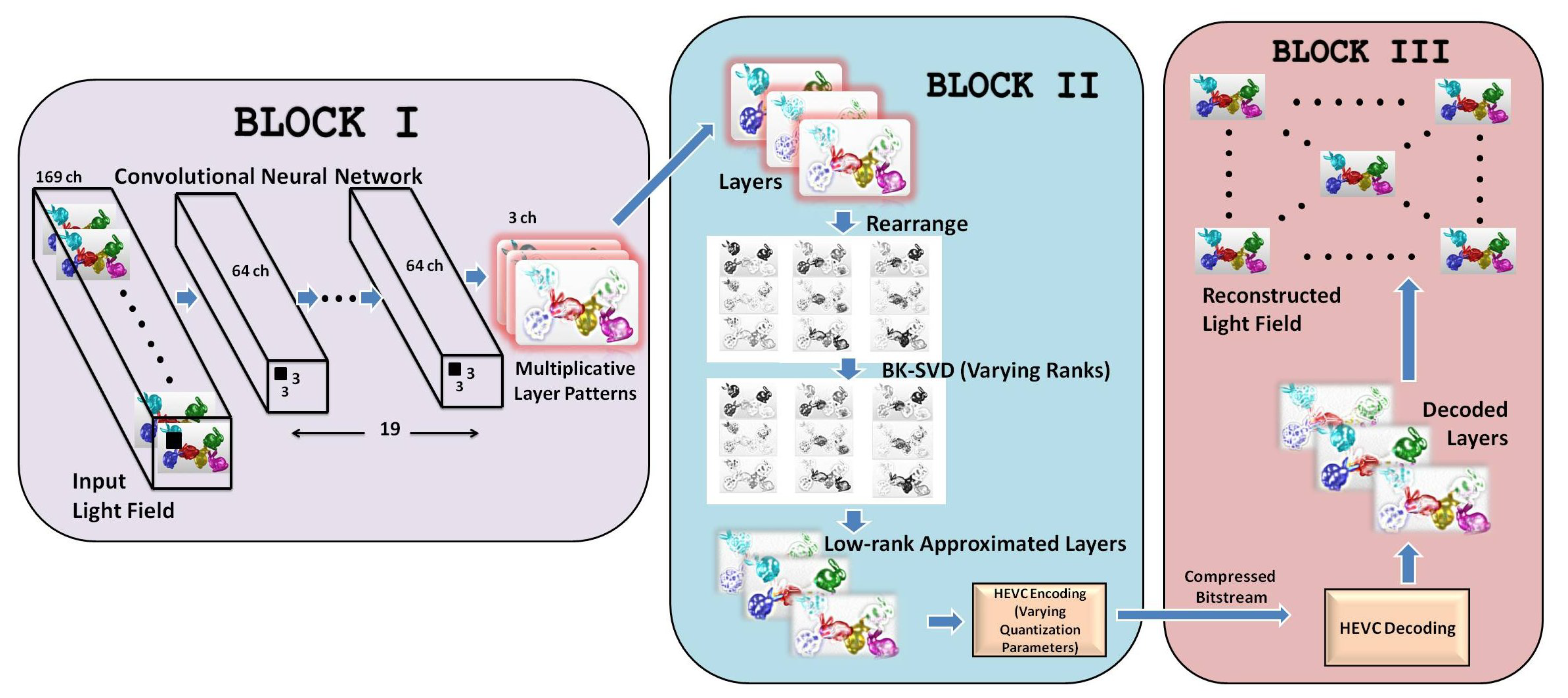
The workflow of our proposed representation and coding scheme is illustrated in Figure 2. The proposed scheme is divided into three major components. The first component (BLOCK I) represents a convolutional neural network that converts the input light field views into three multiplicative layers. In the second component (BLOCK II), the intrinsic redundancy in light field data is efficiently removed by analyzing the hidden low-rank structure of multiplicative layers on a Krylov subspace by varying BK-SVD ranks. This followed by the encoding of low-rank approximated multiplicative layers using HEVC effectively eliminates inter-frame and intra-frame redundancies. In the last component (BLOCK III), the light field is reconstructed from the decoded layers, as depicted in Figure 2. Each component of the proposed representation and compression scheme is described in the following sections.
2.1. Light Field Views to Stacked Multiplicative Layers
In the first component, the proposed scheme generates optimized multiplicative layers from real light field data. The four-dimensional light field is parameterized by the coordinates of the intersections of light rays with two planes [47,48]. The coordinate system is denoted by for the first plane and for the second plane (Figure 1c). In this system, a light ray first intersects the plane at and then the plane at coordinate . The light field is represented by . If the plane is located at depth z, the ray will have coordinates .
Multiplicative layers [5] are light attenuating panels that are stacked in evenly spaced intervals in front of a backlight as shown in Figure 1. The transmittance of a layer is given by and a light ray emitted from this display will have its intensity normalized by the intensity of the backlight and can be expressed as
Here, we assume that a light-field display is composed of three layers located at , where . It must be noted that z corresponds to the disparity among the directional views, rather than the physical length [14]. The multiplicative layers need to be optimized to display a 3-D scene. The optimization goal for the layer patterns is given by
where depicts the light field emitted from the display.
We utilize a CNN to generate optimal multiplicative layers from the input light field images. The CNN-based optimization method proves to be better in terms of the balance between computation time and accuracy than the previous analytical optimization approach based on non-negative tensor factorization (NMF) methods [5,14,17,18]. Analytical methods obtain three multiplicative layers of an input light field by carrying out the optimization one layer at a time and repeating it for all layers until convergence [14]. The solutions are updated in an iterative manner, with a trade-off between computation time (number of iterations) and accuracy of the solution. On the other hand, CNN-based methods are proven to be faster and produce better accuracy, as well [14]. We have discussed the merits of using a convolutional neural network over analytical methods for layer pattern optimization in Section 3.5. Optimization for the three layer patterns from the full light field using CNN can be mapped as
where represents a tensor containing all the pixels of for all .
Similarly, the mappings from the layers patterns to the light field can be rewritten as
where represents all the light rays in . During training, a CNN minimizes the squared error loss given by
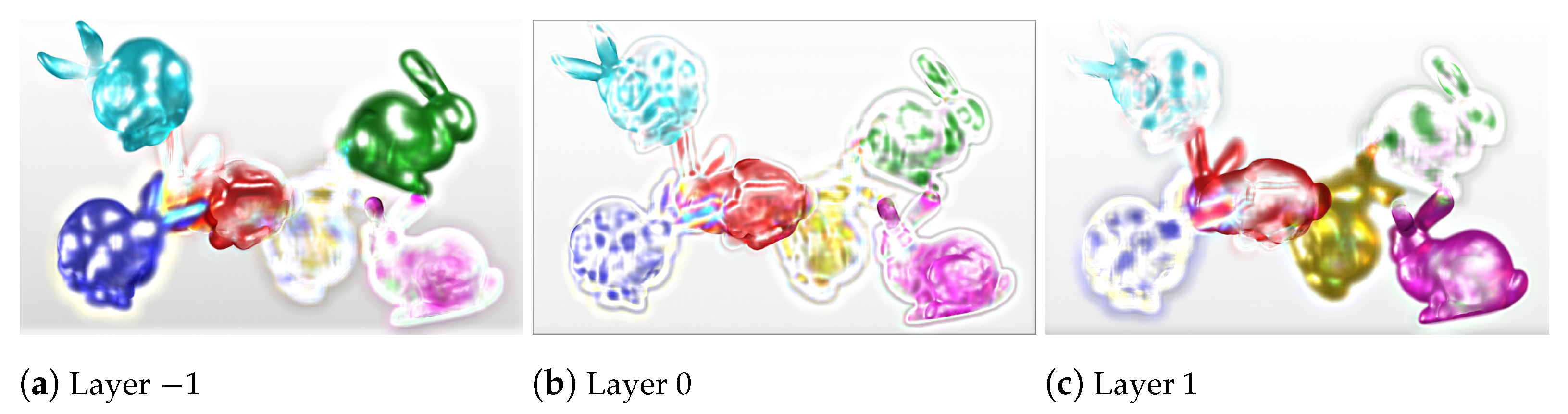
Note that (f()), where f is performed by the CNN to produce the multiplicative layer patterns , and reconstructs light field from . Tensors and have 169 channels corresponding to the 13 × 13 views of the light field image, and tensor has three channels corresponding to the three layer patterns of the multiplicative layered display. The final trained network can convert the input light field views into three optimized output layer patterns. This is the first component in our proposed coding scheme (BLOCK I in Figure 2). Figure 3 illustrates the CNN-produced multiplicative layers of the Bunnies light field [49].
2.2. Low Rank Representation and Coding of Stacked Multiplicative Layers on Krylov Subspace
The key idea of the proposed scheme is to remove the intrinsic redundancy in light field data by analyzing the hidden low-rank structure of multiplicative layers. The second component of our workflow (BLOCK II in Figure 2) involves this low-rank representation of optimized multiplicative layers. We represented the layers compactly on a Krylov subspace and approximated them using Block Krylov singular value decomposition (BK-SVD).
The Randomized Simultaneous Power Iteration method has been popularized to approximate the singular value decomposition (SVD) of matrices [50,51]. This simultaneous iteration approach can optimally achieve the low-rank approximation of a matrix within of optimal for spectral norm error by quickly converging in iterations for any matrix. However, it may not guarantee a strong low-rank approximation or return high-quality principal components of the matrix. To improve this, Cameron Musco and Christopher Musco introduced a simple randomized block Krylov method [52], which can further improve the accuracy and runtime performance of simultaneous iteration. Experimentally, the randomized block Krylov SVD (BK-SVD) performs fairly better in just iterations. The BK-SVD approach is closely related to the classic Block Lanczos algorithm [53,54] and outputs a nearly optimal approximation for any matrix, independent of singular value gaps.
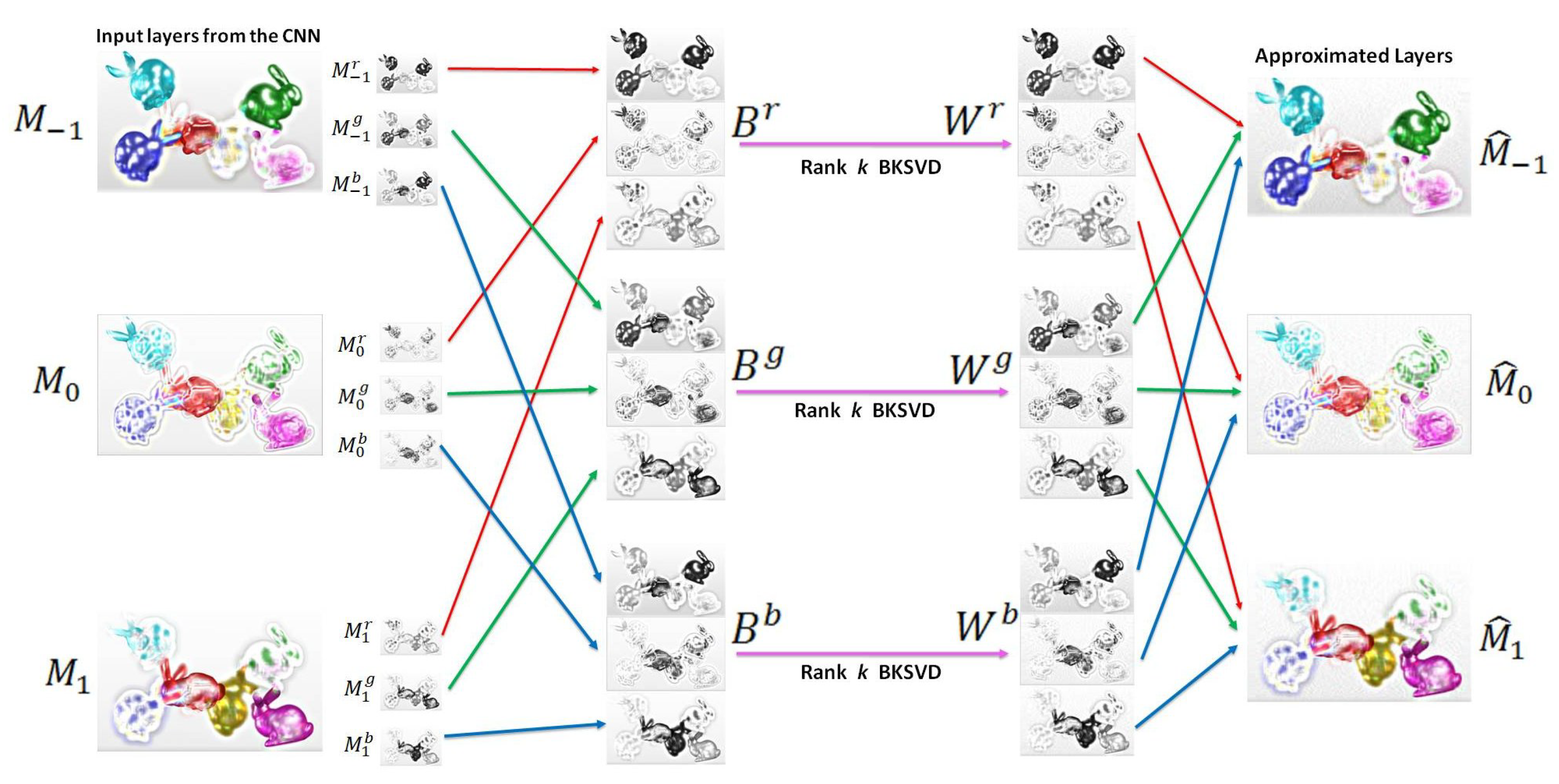
In our proposed scheme, we denote each multiplicative layer pattern produced by the CNN as , where . The red, green, and blue color channels of the layer z are denoted as , , and , respectively. We constructed the matrices , where , as
The intrinsic redundancies in multiplicative layers of the light field can be effectively removed by following low-rank BK-SVD approximation in a Krylov subspace for each , (Figure 4). For simplicity, we will denote as B in the following mathematical formulation.
Given a matrix of rank r, the SVD can be performed as , where the left and right singular vectors of B are the orthonormal columns of and , respectively. is a positive diagonal matrix containing , the singular values of B. Conventional SVD methods are computationally expensive. Thus, there is substantial research done on randomized techniques to achieve optimal low-rank approximation [50,51,52]. The recent focus has shifted towards methods that inherently do not depend on the properties of the matrix or the gaps in its singular values. In our present formulation of low-rank light field layer approximation, we seek to find a subspace that closely captures the variance of B’s top singular vectors and avoids the gap dependence in singular values. We target spectral norm low-rank approximation error of B, which is intuitively stronger. It is defined as
where W is a rank k matrix with orthonormal columns . In a rank k approximation, only the top k singular vectors of B are considered relevant and the spectral norm guarantee ensures that recovers B up to a threshold .
Traditional Simultaneous Power Iteration algorithms for SVD initialized with random start vectors achieve the spectral norm error (7) in nearly iterations. Block Krylov SVD approach presented in Reference [52], a randomized variant of the Block Lanczos algorithm [53,54], guarantees to achieve the same in just iterations. This not only improves runtime for achieving spectral norm error (7), but guarantees substantially better performance in practical situations, where gap independent bound is critical for excellent accuracy and convergence. In the present formulation, we start with a random matrix and perform Block Krylov Iteration by working with the Krylov subspace,
We take advantage of low degree polynomials that allow us to compute fewer powers of B and improve performance with fewer iterations. We construct for any polynomial of degree q by working with Krylov subspace K. The approximation of matrix B done by projecting it onto the span of is similar to the best k rank approximation of B lying in the span of the Krylov space K. Thus, the nearly optimal low-rank approximation of B can be achieved by finding this best rank k approximation. Further, to ensure that the best spectral norm error low-rank approximation lies in a specific subspace (i.e., in the span of K), we orthonormalize the columns of K to obtain using the QR decomposition method [55]. We take SVD of matrix where , for faster computation and accuracy. The rank k approximation of B is matrix W, which is obtained as
where is set to be the top k singular vectors of S. Consequently, the rank k block Krylov approximation of matrices , , and are , , and , respectively. The for every color channel . The approximated layers are obtained by drawing out the color channels from the approximated matrices.
We sectioned out the rows uniformly as
The red, green, and, blue color channels are then combined to form each approximated layer, , , and . These three block Krylov approximated layers are subsequently encoded using HEVC.
2.3. The Encoding of Rank-Approximated Layers
The High Efficiency Video Coding (HEVC) [29] is the latest international standard for video compression. It was standardized by ITU-T Video Coding Experts Group and the ISO/IEC Moving Picture Experts Group. It achieves improved compression performance over its predecessors, with at least a 50% bit-rate reduction for the same perceptual quality.
The encoding algorithm of HEVC flexibly divides each frame of the video sequence into square or rectangular blocks. This block partitioning information is relayed to the decoder. The first video frame is coded using only intra prediction (spatial prediction from other regions of the same frame), and succeeding frames are predicted from one, two, or more reference frames using inter and intra prediction. Motion-compensated prediction is used to remove the temporal redundancy during inter prediction.
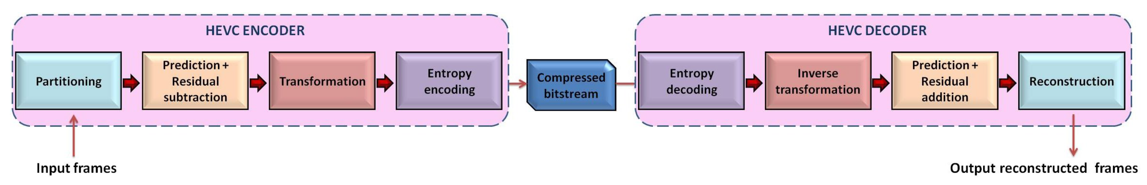
In our proposed scheme, we converted the block Krylov approximated layers into the YUV420 format. We then used HEVC encoder for various QPs to remove inter and intra redundancies of the low-rank approximated layers and compress them into a bitstream. A linear spatial transform is applied to the residual signal information between the intra or inter predictions. The transform coefficients are then scaled and quantized. The HEVC performs quantization of the coefficients using QP values in the range of 0–51. To make the mapping of QP values to the step sizes approximately logarithmic, the quantizer doubles step size each time the QP value increases by 6. The scaled and quantized transform coefficients are entropy coded and transmitted to the decoder along with the prediction information. The workflow of the entire encoding process is depicted in Figure 5.
2.4. The Decoding and Reconstruction of the Light Field
This section reports the decoding procedure of compressed layers and the reconstruction of light field (BLOCK III in Figure 2). The HEVC decoder performs entropy decoding of the received bitstream. It then reconstructs the quantized transform coefficients by inverse scaling and inversely transforming the residual signal approximation. The residual signal is added to the prediction, and this result is fed to filters to smooth out the artifacts introduced because of the block-wise processing and quantization. Finally, the predicted frames are stored in the decoder buffer to predict successive frames.
We decoded three layers from the bitstream and converted them into the RGB format. The decoded layers are denoted as , where depicts the depth of the layers.
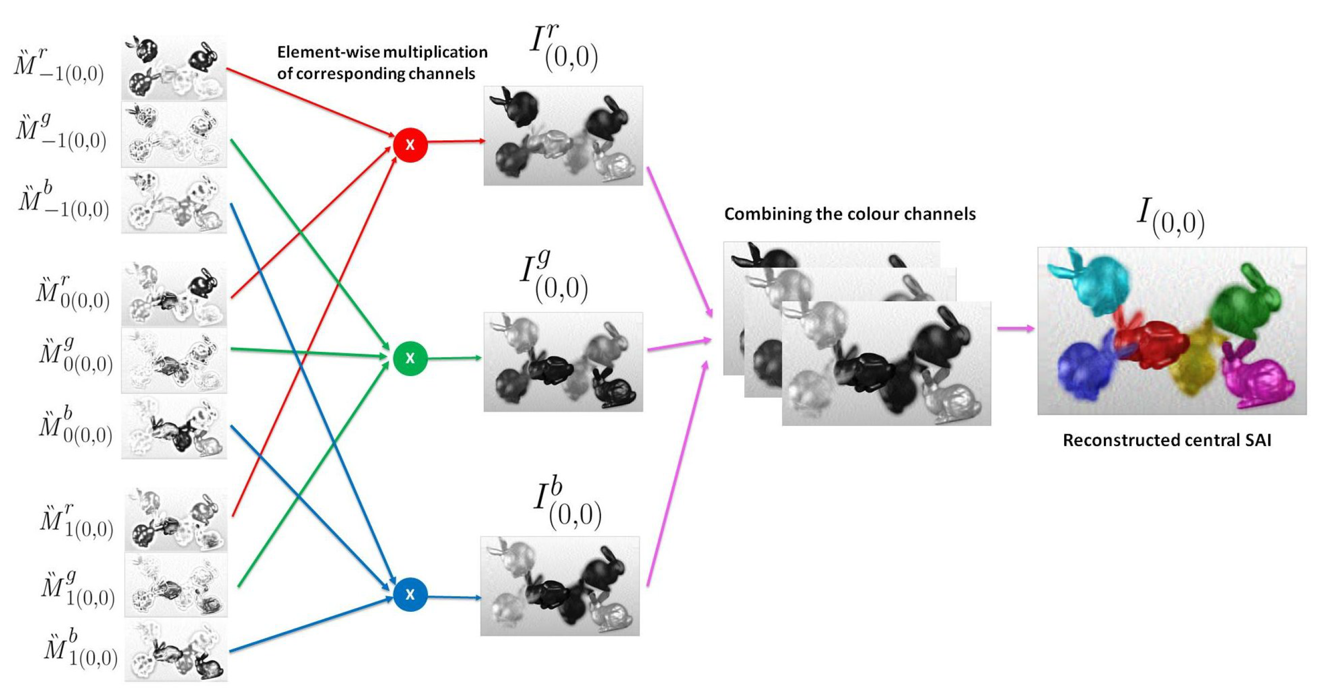
The SAIs are reconstructed from these decoded layers in the following way. Let be the sub-aperture image at the viewpoint and the intensity at pixel location be , where and , . Since we aim to reconstruct the inner 13 × 13 views of the light field, are integers such that . This SAI is obtained by translating the decoded layers to and performing an element-wise product of the color channels of the translated layers. For a particular view , the translation of every zth layer , to is carried out as
Thus, the three translated layers for every viewpoint are
An element-wise product of each color channel , of the translated layers gives the corresponding color channel of the sub-aperture image.
The combined red, green and blue color channels output the reconstructed light field sub-aperture image at the viewpoint as . Figure 6 illustrates the reconstruction of the central light field view for . All the 169 light field views are similarly reconstructed. The pseudo code of the proposed scheme is given in Algorithm 1. The main steps of BK-SVD decomposition are summarized in Algorithm 2.
| Algorithm 1:Proposed scheme | |
Input: Light Field | |
Output: Reconstructed SAIs , , | |
| 1 | Extract SAIs from Light Field: SAIs |
| 2 | Transform SAIs to multiplicative layers using CNN: SAIs |
| 3 | |
| 4 | Find low-rank approximation: Algorithm 2 (, ) |
| 5 | Rearrange and obtain approximated layers: |
| 6 | HEVC encode the approximated layers |
| 7 | HEVC decode |
| 8 | Translate for every view : |
| 9 | Obtain color channel of SAI: |
| 10 | Combine the color channels to reconstruct the SAIs: |
| Algorithm 2:Block Krylov Singular Value Decomposition | |
Input: , error , rank | |
Output: | |
| 1 | , |
| 2 | |
| 3 | Orthonormalize the columns of to obtain |
| 4 | Compute |
| 5 | Set to the top k singular vectors of . |
| 6 | return |
3. Results and Analysis
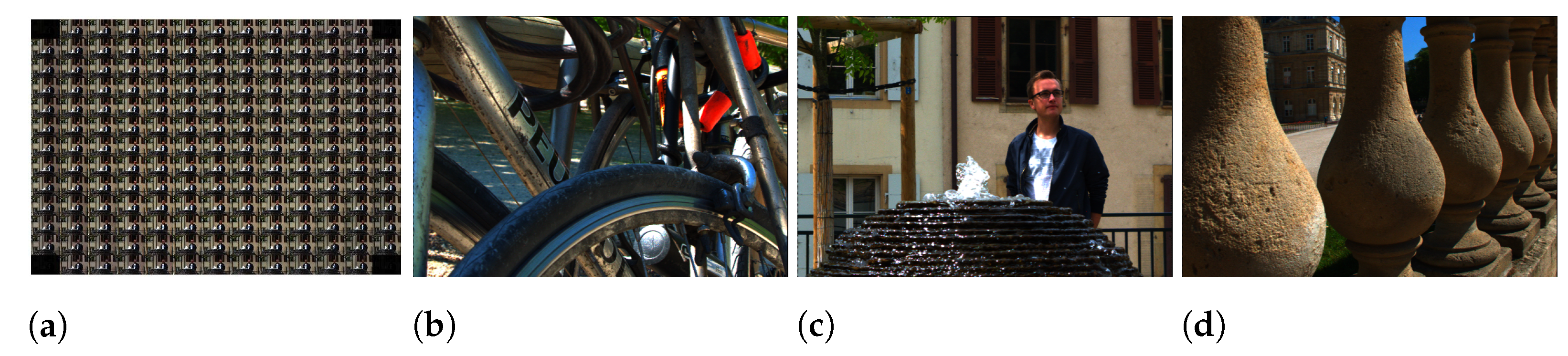
The performance of the proposed compression scheme was evaluated on real light fields captured by plenoptic cameras. We experimented with Bikes, Fountain-Vincent2, and Stone-Pillars Outside light field images from the EPFL Lightfield JPEG Pleno database [56]. The raw plenoptic images were extracted into 15 × 15 sub-aperture images (each with a resolution of 434 × 625 pixels) using MATLAB Light field toolbox [57]. In Liu et al. [23] and Ahmad et al. [25], only the central 13 × 13 views of the light field were considered as the pseudo sequence for compression. The border SAIs suffer from severe geometric distortion (due to light field lenslet structure) and blurring, and they are less useful in recovering the light field. To facilitate a fair comparison with these state-of-the-art coding methods, we have also discarded the border SAIs and only considered the inner 13 × 13 light field views for our tests. Figure 7 shows the extracted views and the central views of the chosen light field images.
3.1. Experimental Settings of CNN
In the first component of the proposed coding scheme (BLOCK I in Figure 2), a convolutional neural network learns the optimized multiplicative layers from real light field data. We experimented on the 5 × 5 Bunnies dataset [49] to analyze the CNN learning for various hyperparameters. The model was trained with all the following combinations:
- Learning rate (LR): 0.001, 0.0001, 0.00001;
- Batch size (BS): 15, 30;
- Number of epochs (E): 5, 10, 15, 20.
Apart from these combinations of hyperparameters, we analyzed the influence of the network on results by varying the number of convolutional layers as 15, 20, and 25. Maruyama et al. [14] had demonstrated 3 × 3 as an optimal filter size in the network and used 64 channels for the intermediate feature maps. We also chose the same filter size and number of channels in the intermediate layers.
Figure 8a presents the training results of the experiment with 20 convolutional layers in the CNN. We examined similar hyperparameter variation plots for 15 and 25 convolutional layers and concluded that LR 0.0001, BS 15, and E 20 give optimal PSNR results in BLOCK I of the proposed scheme. The multiplicative layers produced by the 15, 20, and 25 convolutional layered networks with these choices of hyperparameters were further passed to BLOCK II of the proposed coding scheme. We performed the BK-SVD (for ranks 20 and 60) and HEVC step (with QPs 2, 6, 10, 14, 20, 26, 38). Figure 8b–d display the corresponding bitrate versus PSNR results. Thus, we inferred a suitable model for the proposed scheme by choosing 20 convolutional layers and trained the CNN for 20 epochs at a learning rate of 0.0001, and a batch size of 15. Multiplicative layers produced using this model for Bunnies are shown in Figure 3.
The multiplicative layers can further be fed into BLOCK II (BK-SVD step + HEVC) for compression. The proposed coding scheme achieves flexible bitrates for the various ranks of BK-SVD of multiplicative layers and varying HEVC quantization parameters. Thus, it realizes the goal of covering a range of multiple bitrates using a single CNN model.
3.2. Implementation Details of Proposed Scheme
We implemented the proposed coding scheme on a single high-end HP OMEN X 15-DG0018TX Gaming laptop with 9th Gen i7-9750H, 16 GB RAM, RTX 2080 8 GB Graphics, and Windows 10 operating system. The multiplicative layer patterns for input light fields Bikes, Fountain-Vincent2, and Stone-Pillars Outside were optimized using the chosen CNN with 20 2-D convolutional layers stacked in a sequence. The network was trained (learning rate 0.0001, batch size 25, 20 epochs) with 30 training images generated from light fields Friends 1, Poppies, University, Desktop, and Flowers, from the EPFL Lightfield JPEG Pleno database [56]. Each training sample was a set of 169 2-D image blocks with 64 × 64 pixels extracted from the same spatial positions in a light-field dataset. We implemented the entire network using the Python-based framework, Chainer (version 7.7.0).
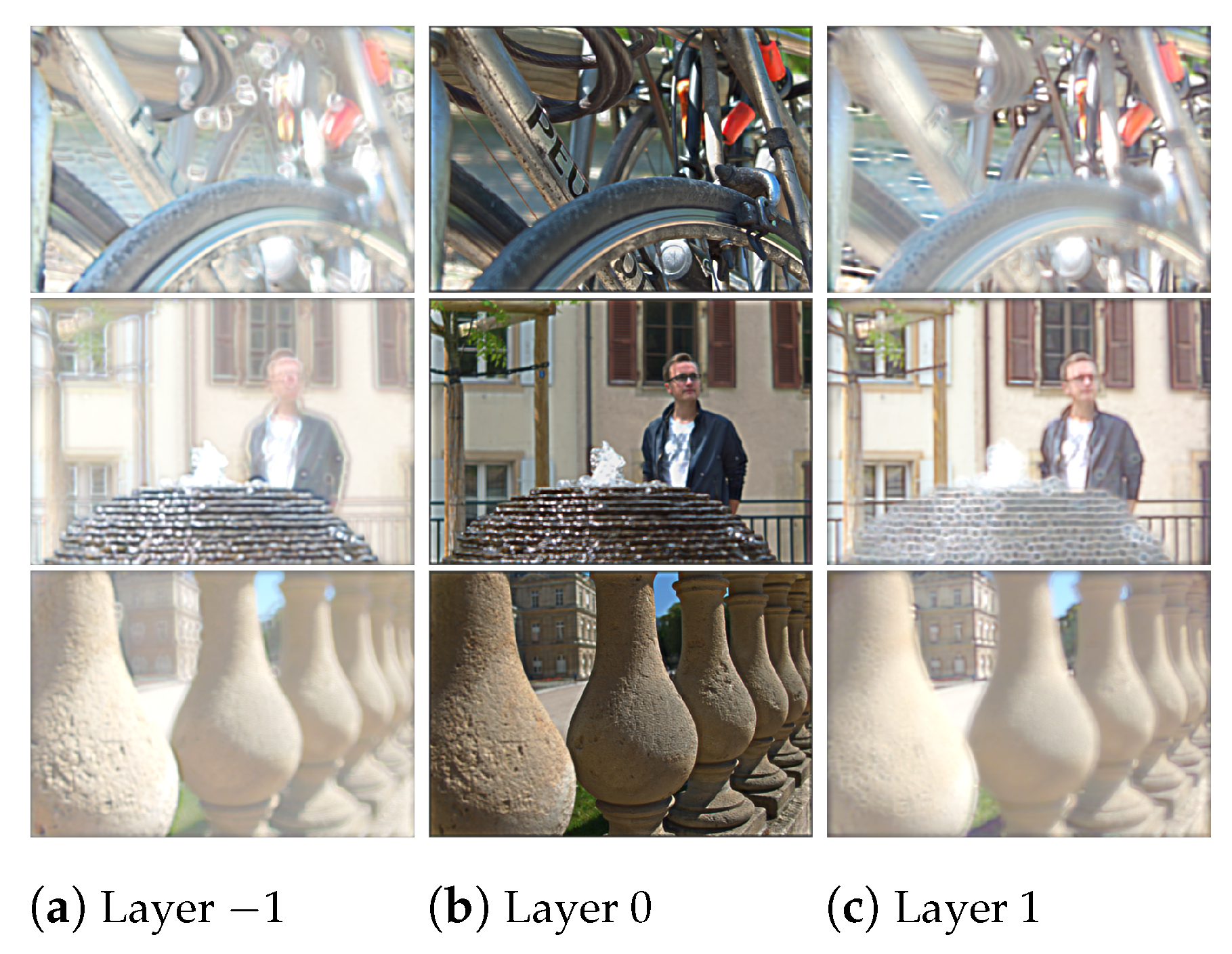
During training, the CNN (in BLOCK I of Figure 2) solves the optimization problem (Equation (5)) by computing loss as the mean square difference between the original light field and the light field reconstructed from multiplicative layers. The optimal multiplicative layers are learned as a result of the optimization of the loss function and this eliminates the need for any ground truth information. The resultant output layers for the Bikes, Fountain-Vincent2, and Stone-Pillars Outside light field images, obtained from the trained CNN model are presented in Figure 9. We rearranged the color channels of these multiplicative layers as described in Section 2.2. We then applied BK-SVD for ranks 4 to 60 (incremented in steps of four) and computed 50 iterations for each rank. The approximated matrices were then rearranged back into layers and converted into the YUV420 color space.
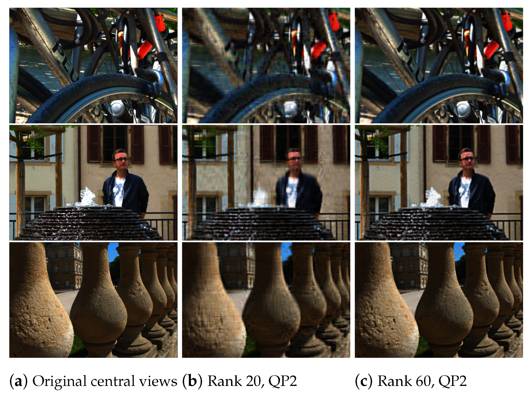
For the HEVC step, we used 32 bit HM encoder (version 11.0) to compress all the YUV files of different approximated ranks. We choose seven quantization parameters, QP 2, 6, 10, 14, 20, 26, and 38, to test both high and low bitrate cases. The encoder compression produces a bitstream for a fixed rank and QP, that can be stored or transmitted. We followed the reverse procedure on the compressed bitstream to reconstruct the 13 × 13 views of the light fields. The HM decoder is used to recover the files in the YUV420 format, which are then converted back to the RGB color space. The three decoded layers are used to reconstruct the entire sub-aperture images of the light field. A comparison of the original central view of the Bikes, Fountain-Vincent2, and Stone-Pillars Outside light field images and the reconstructed central light field views is shown in Figure 10.
3.3. Results and Comparative Analysis
The performance of our proposed coding scheme is compared to previous pseudo-sequence-based compression schemes [23,25], the HEVC software (version 11.0) [29], and the JPEG standard [58]. We subjected all these anchor schemes to the same test conditions and quantization parameters (QPs-2, 6, 10, 14, 20, and 38) as used in our experimental settings. All PSNR-bitrate graphs are shown in Figure 11 and Figure 12. The total number of bytes written to file during compression by these four anchors is documented in Table 1. Total number of bytes used by the proposed coding scheme for various ranks is summarized in Table 2.
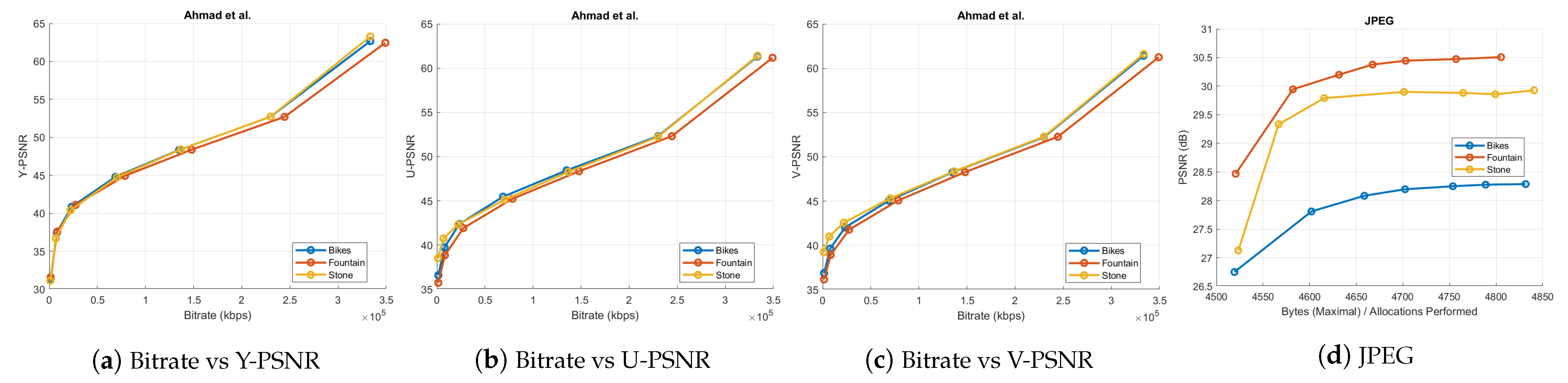
Ahmad et al. [25] interpreted the sub-aperture views of the light field as frames in a multi-view sequence. They availed the tools in the multi-view extension of HEVC to exploit the 2D inter-view correlation among the views. We used the PPM color image format of the inner 13 × 13 views of the Bikes, Fountain-Vincent2, and Stone-Pillars Outside light field images to evaluate this multi-view compression algorithm. The bitrate versus PSNR results of Ahmad et al. is shown in Figure 11a–c. We coded the input SAIs of the chosen light field data with the legacy JPEG [58], as well. The corresponding bytes per allocation performed versus PSNR curve is in Figure 11d.
Liu et al. [23] formulated a predictive coding approach and treated light field views as a pseudo-sequence-like video. They compressed the central view first and then the remaining views in a symmetric, 2D hierarchical order. Motion estimation and compensation in video coding systems were reused to perform inter-view prediction. Due to the public unavailability of Liu et al.’s lenslet YUV files for datasets apart from Bikes, we analyzed their compression performance [23] on the 13 × 13 SAIs of Bikes only. The total number of bytes used in compression using this approach is given in Table 1.
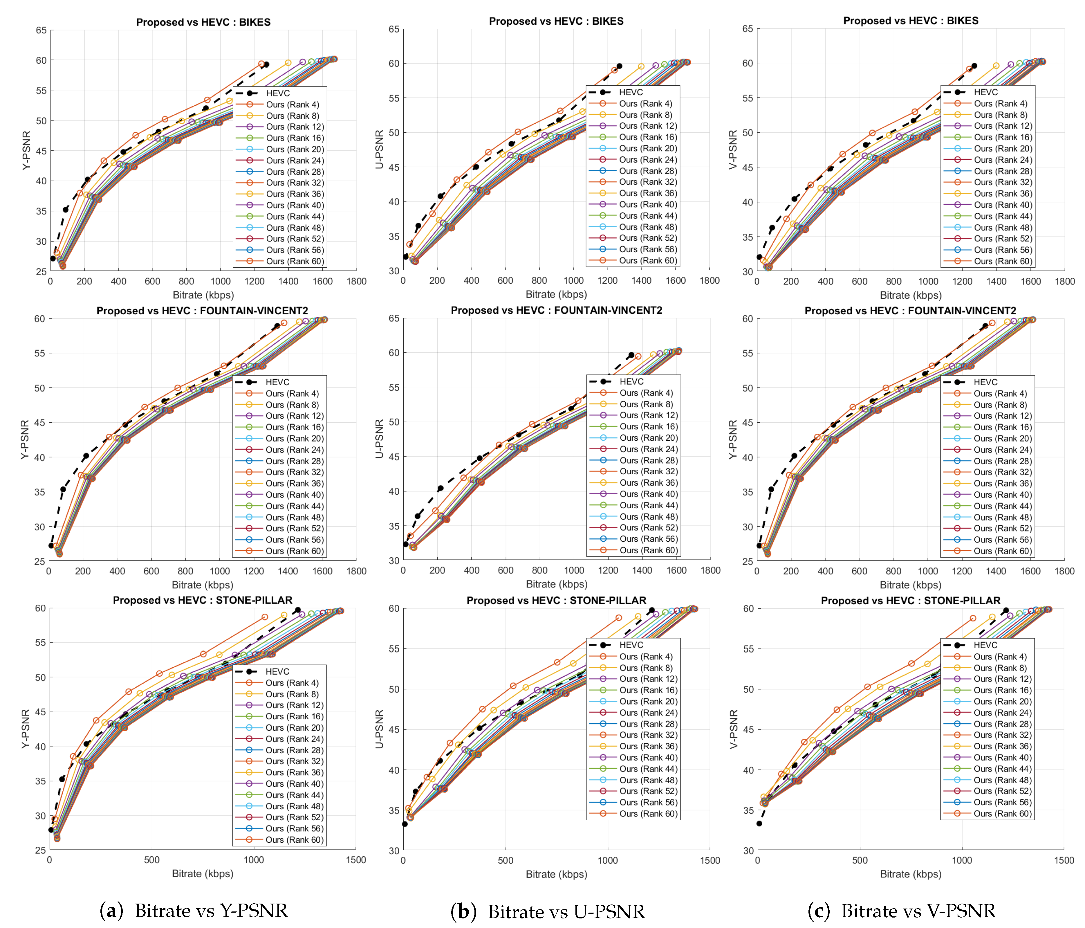
To evaluate the HEVC [29] performance, the 169 SAIs in YUV420 color space were directly fed into the 32 bit HM codec (version 11.0) for the same chosen QPs. The rate-distortion graphs comparing HEVC with the proposed scheme is shown in Figure 12. Bitrates in case of Ahmad et al. [25] are in the order of . Hence, these results are plotted separately in Figure 11a–c because of the scale mismatch with bitrates of our proposed scheme. In addition, in case of JPEG, we have shown the maximal bytes per allocations performed versus PSNR plot (Figure 11d) and the x-axis is not the same as in Figure 12. Thus, for a fair comparison, we have not plotted the results of the proposed coding scheme and JPEG together. The proposed coding scheme consistently outperforms on all datasets.
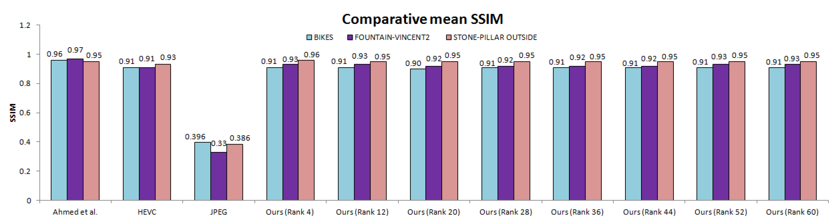
The total number of bytes taken by our approach is comparatively much less than other anchors (Table 1 and Table 2) for both lower and higher ranks. We also computed SSIM (Structural Similarity Index) scores for all 13 × 13 views of scenes. Figure 13 illustrates the comparative mean SSIM values of the proposed coding scheme and results of Ahmad et al. [25], HEVC [29], and JPEG [58] codecs. We saved significant bitrates at different ranks and maintain good reconstruction quality.
Further, we performed an objective assessment using the Bjontegaard [59] metric. This metric can compare the performance of two different coding techniques. We compared bitrate reduction (BD-rate) of proposed scheme with respect to Ahmed et al., Liu et al., and HEVC codec. The average percent difference in rate change is estimated over a range of quantization parameters for the fifteen chosen ranks.
A comparison of the percentage of bitrate savings of our proposed coding scheme with respect to the anchor methods for the Bikes, Fountain-Vincent2, and the Stone-Pillars Outside datasets are shown in Table 3, Table 4 and Table 5, respectively. On Bikes data, the proposed scheme achieves , , and bitrate reduction compared to Ahmad et al., HEVC, and Liu et al., respectively (Table 3). On Fountain-Vincent2 data, we noticed and bitrate savings compared to Ahmad et al. and HEVC codec, respectively (Table 4). On Stone-Pillars Outside data, we achieve and bitrate reduction compared to Ahmad et al. and HEVC, respectively (Table 5).
3.4. Advantages of Using Multiplicative Layers
The proposed scheme generates three optimal multiplicative layers of input light field for layered light field displays. There is a clear advantage to approximate and encode just the three multiplicative layers rather than the entire set of light field views in terms of computation speed, bytes written to file during compression, bitrate savings with respect to state-of-the-art coding methods, as well as SSIM performance. To analyze this, we experimented by directly feeding all 13 × 13 views of the Bikes light field into BLOCK II of the proposed coding scheme (AV(169)). These results were then compared with usage of just 3 multiplicative layers described in the previous sections (ML(3)). Block-Krylov low rank approximation was done for ranks 20 and 60, followed by HEVC encoding for quantization parameters 2, 6, 10, 14, 20, and 38.
We noted the computation time for each step in BLOCK II. Table 6 highlights the results. Evidently, the proposed compression scheme works much faster with just three light field multiplicative layers. This proves to be advantageous over using all views of the light field. We have also compared the number of bytes written to file during compression in Table 7, where a higher number of bytes in case of AV(169) can be observed. The bitrate reduction of ML(3) and AV(169) with respect to Liu et al. [23], HEVC codec [29], and Ahmed et al. [25] (estimated over a range of quantization parameters 2, 6, 10, 14, 20, 26, 38 for ranks 20 and 60) is depicted in Table 8.
To evaluate the decoding module of the proposed scheme (BLOCK III), we used the SSIM metric to compare decoded views of experiment AV(169) and ML(3). Mean SSIM over the decoded views was calculated for each QP result and each rank of Bikes. These SSIM comparison graphs are illustrated in Figure 14. The proposed scheme with three multiplicative layers performs better perceptually, as well, since the matrix constructed to perform BK-SVD in case of AV(169) is larger in size. The approximation quality deteriorates when all 13 × 13 views are simultaneously considered.
3.5. Advantages of Using CNN over Analytical Methods in BLOCK I
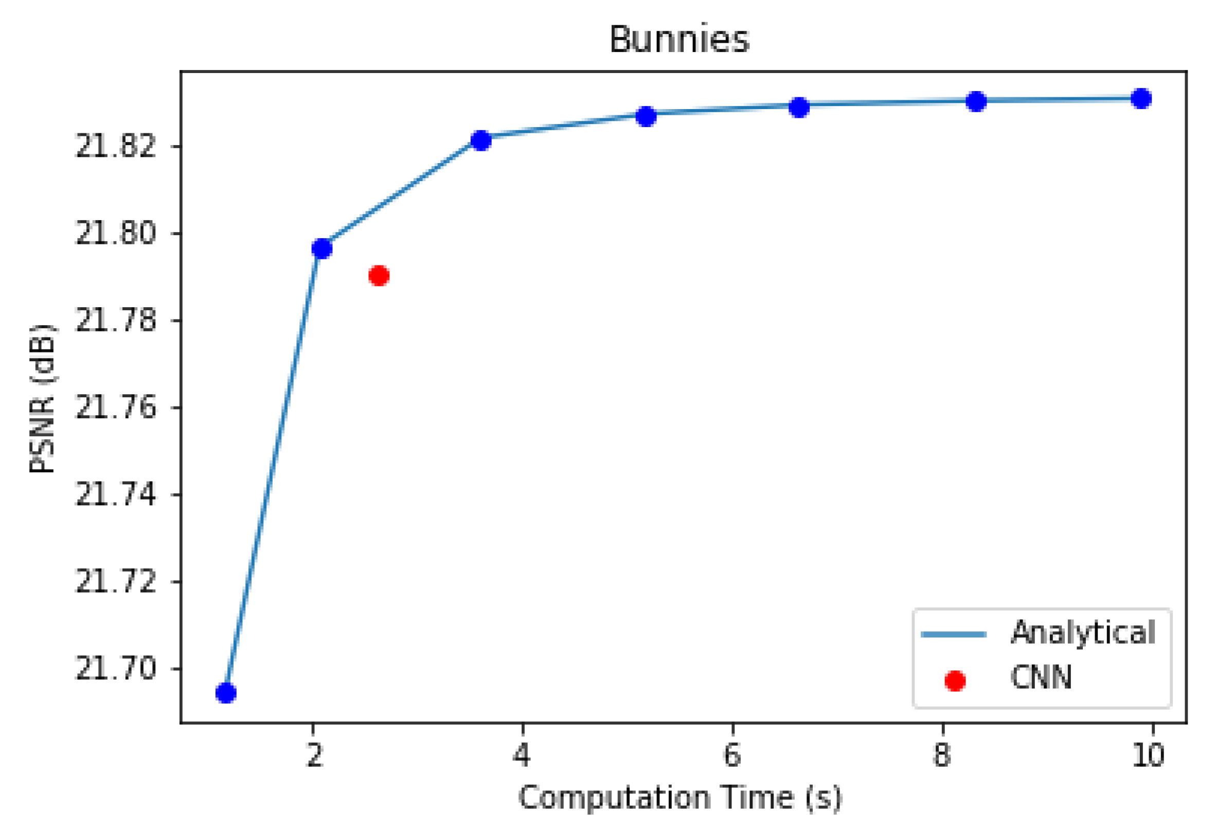
In the first component of the proposed coding scheme, the multiplicative layered representation of the light field is generated. This can be done analytically one layer at a time, with repetition until the solution of Equation (2) converges, or by using a CNN [14]. We experimented with the 5 × 5 Bunnies dataset [49] to compare the performance of the CNN and analytical optimization method to obtain three optimal multiplicative layers. The analytical method was evaluated for 10, 25, 50, 75, 100, 125, and 150 iterations. The CNN used was trained with 20 2-D convolutional layers for 20 epochs at a learning rate of 0.0001 and a batch size of 15. Figure 15 illustrates the PSNR versus computation time plot of this experiment.
In case of the analytical approach, accuracy gradually increases with computation time. The inference time for the CNN in Figure 15 is marginally slower than that of the analytical method for the same PSNR performance in our experiment. Nevertheless, Maruyama et al. [14] have demonstrated that, with better GPUs and more training data, CNN inference can be performed much faster than the analytical method for the same reconstruction quality.
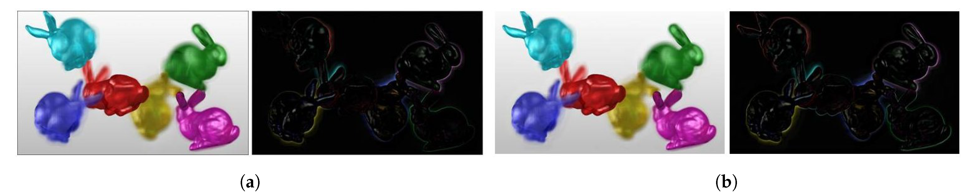
We have also shown view 19 of the BLOCK I reproduced Bunnies light field using analytical and CNN methods, along with their error images, in Figure 16. The CNN results are better in this case in terms of PSNR and SSIM scores, as well. Thus, we prefer the CNN over the analytical method in BLOCK I of the proposed coding scheme as it strikes a better balance between computation speed and accuracy.
4. Conclusions
We proposed an efficient representation and novel lossy compression scheme for layered light-field displays with light-ray operations regulated using multiplicative layers and a CNN-based method. A single CNN model is employed to learn the optimized multiplicative layer patterns. A light field is compactly (compressed) represented on a Krylov subspace, considering the transmittance patterns of such a few layers and approximation derived by Block Krylov SVD. Factorization derived from BK-SVD exploits spatial correlation in multiplicative layer patterns with varying low ranks. Further, encoding with HEVC eliminates the inter-layer and intra-layer redundancies in the low-rank approximated representation. By choosing varying ranks and quantization parameters, the scheme is flexible to adjust the bit rates in the layered representation with a single CNN. Consequently, it realizes the goal of covering a range of multiple bitrates within a single trained CNN model. The experiments with benchmark light field datasets exhibit very competitive results.
This critical characteristic of the proposed scheme sets it apart from other existing light field coding methods which train a system (or network) to support only specific bitrates during the compression. Moreover, current solutions are not specifically designed to target layered displays. Broadly, compression approaches are classified to work for lenslet-based formats or sub-aperture images based pseudo-sequence representation. Our proposed scheme could flexibly work with different light-ray operations (multiplication and addition) and analytical or data-driven CNN-based methods, targeting multi-layered displays. It is adaptable for a variety of multi-view/light field displays. In addition, it can complement existing light-field coding schemes, which employ different networks to encode light field images at different bit rates. This would enable deploying the concept of layered displays on different auto-stereoscopic platforms. One can optimize the bandwidth for a given target bit-rate and deliver the 3D contents with limited hardware resources to best meet the viewers’ preferences.
Our future work span in several directions. We will further extend the proposed idea to light field displays, such as ones with more than three light attenuating layers, projection-based, and holographic displays with optical elements constructed using additive layers. Proof-of-concept experiments with our scheme pave way to form a deeper understanding in the rank-analysis of a light field using other mathematically valid tensor-based models and efficient layered representations for 3D displays. Another interesting direction is to extend the proposed mathematical formulation for coded mask cameras useful in compression of dynamic light field contents or a focal stack instead of processing multi-view images in layered displays. We aim to verify our scheme with not only computer simulations, but with a physical light field display hardware. In addition, we will consider the aspect of human perception by performing a subjective analysis of perceptual quality on a light field display. The proposed algorithm uses RGB space in which all channels are equally important. For image perception, there are better color spaces, like HSV/HSL or Lab. Analyzing other color spaces would be worth considering in further work.
Author Contributions
Conceptualization, M.S.; Data curation, J.R., M.S. and P.G.; Formal analysis, J.R. and M.S.; Funding acquisition, M.S.; Investigation, J.R., M.S. and P.G.; Methodology, M.S.; Project administration, J.R. and M.S.; Resources, M.S.; Software, J.R., M.S. and P.G.; Supervision, M.S.; Validation, J.R. and M.S.; Visualization, J.R.; Writing—Original draft, J.R. and M.S.; Writing—Review & editing; J.R. and M.S. All authors have read and agreed to the published version of the manuscript.
Funding
The scientific efforts leading to the results reported in this paper were supported in part by the Department of Science and Technology, Government of India under Grant DST/INSPIRE/04/2017/001853.
Institutional Review Board Statement
Not applicable.
Informed Consent Statement
Not applicable.
Data Availability Statement
Not applicable.
Acknowledgments
We would like to thank Uma T.V. for her help in setting up the required Python environment and libraries for the running of our codes.
Conflicts of Interest
The authors declare no conflict of interest.
Abbreviations
The following abbreviations are used in this manuscript:
| LCD | Liquid crystal display |
| CNN | Convolutional neural network |
| BK-SVD | Block Krylov singular value decomposition |
| HEVC | High efficiency video coding |
| QP | Quantization parameter |
| HOE | Holographic optical element |
| HLRA | Homography-based low-rank approximation |
| GNN | Gaussian neural network |
| SAI | Sub-aperture image |
| PSNR | Peak signal-to-noise ratio |
| SSIM | Structural similarity index |
References
- Surman, P.; Sun, X.W. Towards the reality of 3D imaging and display. In Proceedings of the 2014 3DTV-Conference: The True Vision-Capture, Transmission and Display of 3D Video (3DTV-CON), Budapest, Hungary, 2–4 July 2014; pp. 1–4. [Google Scholar]
- Li, T.; Huang, Q.; Alfaro, S.; Supikov, A.; Ratcliff, J.; Grover, G.; Azuma, R. Light-Field Displays: A View-Dependent Approach. In Proceedings of the ACM SIGGRAPH 2020 Emerging Technologies, Online. 17–28 August 2020; pp. 1–2. [Google Scholar]
- Watanabe, H.; Okaichi, N.; Omura, T.; Kano, M.; Sasaki, H.; Kawakita, M. Aktina Vision: Full-parallax three-dimensional display with 100 million light rays. Sci. Rep. 2019, 9, 17688. [Google Scholar] [CrossRef]
- Geng, J. Three-dimensional display technologies. Adv. Opt. Photonics 2013, 5, 456–535. [Google Scholar] [CrossRef] [PubMed] [Green Version]
- Wetzstein, G.; Lanman, D.R.; Hirsch, M.W.; Raskar, R. Tensor Displays: Compressive Light Field Synthesis Using Multilayer Displays with Directional Backlighting. ACM Trans. Graph. 2012, 31, 80. [Google Scholar] [CrossRef]
- Sharma, M.; Chaudhury, S.; Lall, B. A novel hybrid kinect-variety-based high-quality multiview rendering scheme for glass-free 3D displays. IEEE Trans. Circuits Syst. Video Technol. 2016, 27, 2098–2117. [Google Scholar] [CrossRef]
- Sharma, M.; Chaudhury, S.; Lall, B.; Venkatesh, M. A flexible architecture for multi-view 3DTV based on uncalibrated cameras. J. Vis. Commun. Image Represent. 2014, 25, 599–621. [Google Scholar] [CrossRef]
- Sharma, M. Uncalibrated Camera Based Content Generation for 3D Multi-View Displays. Ph.D. Thesis, Indian Institute of Technology Delhi, New Delhi, India, 2017. [Google Scholar]
- Hirsch, M.; Wetzstein, G.; Raskar, R. A compressive light field projection system. ACM Trans. Graph. 2014, 33, 1–12. [Google Scholar] [CrossRef] [Green Version]
- Balogh, T.; Kovács, P.T.; Barsi, A. Holovizio 3D display system. In Proceedings of the 2007 3DTV Conference, Kos, Greece, 7–9 May 2007; pp. 1–4. [Google Scholar]
- Takahashi, K.; Saito, T.; Tehrani, M.P.; Fujii, T. Rank analysis of a light field for dual-layer 3D displays. In Proceedings of the 2015 IEEE International Conference on Image Processing (ICIP), Quebec City, QC, Canada, 27–30 September 2015; pp. 4634–4638. [Google Scholar]
- Saito, T.; Kobayashi, Y.; Takahashi, K.; Fujii, T. Displaying real-world light fields with stacked multiplicative layers: Requirement and data conversion for input multiview images. J. Disp. Technol. 2016, 12, 1290–1300. [Google Scholar] [CrossRef]
- Kobayashi, Y.; Takahashi, K.; Fujii, T. From focal stacks to tensor display: A method for light field visualization without multi-view images. In Proceedings of the 2017 IEEE International Conference on Acoustics, Speech and Signal Processing (ICASSP), New Orleans, LA, USA, 5–9 March 2017; pp. 2007–2011. [Google Scholar]
- Maruyama, K.; Takahashi, K.; Fujii, T. Comparison of Layer Operations and Optimization Methods for Light Field Display. IEEE Access 2020, 8, 38767–38775. [Google Scholar] [CrossRef]
- Kobayashi, Y.; Kondo, S.; Takahashi, K.; Fujii, T. A 3-D display pipeline: Capture, factorize, and display the light field of a real 3-D scene. ITE Trans. Media Technol. Appl. 2017, 5, 88–95. [Google Scholar] [CrossRef] [Green Version]
- Takahashi, K.; Kobayashi, Y.; Fujii, T. From focal stack to tensor light-field display. IEEE Trans. Image Process. 2018, 27, 4571–4584. [Google Scholar] [CrossRef]
- Maruyama, K.; Inagaki, Y.; Takahashi, K.; Fujii, T.; Nagahara, H. A 3-D display pipeline from coded-aperture camera to tensor light-field display through CNN. In Proceedings of the 2019 IEEE International Conference on Image Processing (ICIP), Taipei, Taiwan, 22–25 September 2019; pp. 1064–1068. [Google Scholar]
- Lee, S.; Jang, C.; Moon, S.; Cho, J.; Lee, B. Additive light field displays: Realization of augmented reality with holographic optical elements. ACM Trans. Graph. 2016, 35, 1–13. [Google Scholar] [CrossRef]
- Thumuluri, V.; Sharma, M. A Unified Deep Learning Approach for Foveated Rendering & Novel View Synthesis from Sparse RGB-D Light Fields. In Proceedings of the 2020 International Conference on 3D Immersion (IC3D 2020), Brussels, Belgium, 15 December 2020. [Google Scholar]
- Heide, F.; Lanman, D.; Reddy, D.; Kautz, J.; Pulli, K.; Luebke, D. Cascaded displays: Spatiotemporal superresolution using offset pixel layers. ACM Trans. Graph. 2014, 33, 1–11. [Google Scholar] [CrossRef]
- Hung, F.C. The Light Field Stereoscope: Immersive Computer Graphics via Factored Near-Eye Light Field Displays with Focus Cues. ACM Trans. Graph. 2015, 34, 60. [Google Scholar] [CrossRef]
- Maruyama, K.; Kojima, H.; Takahashi, K.; Fujii, T. Implementation of Table-Top Light-Field Display. In Proceedings of the International Display Workshops (IDW 2018), Nagoya, Japan, 12–14 December 2018. [Google Scholar]
- Liu, D.; Wang, L.; Li, L.; Xiong, Z.; Wu, F.; Zeng, W. Pseudo-sequence-based light field image compression. In Proceedings of the 2016 IEEE International Conference on Multimedia & Expo Workshops (ICMEW), Seattle, WA, USA, 11–15 July 2016; pp. 1–4. [Google Scholar]
- Li, L.; Li, Z.; Li, B.; Liu, D.; Li, H. Pseudo-sequence-based 2-D hierarchical coding structure for light-field image compression. IEEE J. Sel. Top. Signal Process. 2017, 11, 1107–1119. [Google Scholar] [CrossRef] [Green Version]
- Ahmad, W.; Olsson, R.; Sjöström, M. Interpreting plenoptic images as multi-view sequences for improved compression. In Proceedings of the 2017 IEEE International Conference on Image Processing (ICIP), Beijing, China, 17–20 September 2017; pp. 4557–4561. [Google Scholar]
- Ahmad, W.; Ghafoor, M.; Tariq, S.A.; Hassan, A.; Sjöström, M.; Olsson, R. Computationally efficient light field image compression using a multiview HEVC framework. IEEE Access 2019, 7, 143002–143014. [Google Scholar] [CrossRef]
- Gu, J.; Guo, B.; Wen, J. High efficiency light field compression via virtual reference and hierarchical MV-HEVC. In Proceedings of the 2019 IEEE International Conference on Multimedia and Expo (ICME), Shanghai, China, 8–12 July 2019; pp. 344–349. [Google Scholar]
- Sharma, M.; Ragavan, G. A Novel Randomize Hierarchical Extension of MV-HEVC for Improved Light Field Compression. In Proceedings of the 2019 International Conference on 3D Immersion (IC3D), Brussels, Belgium, 11 December 2019; pp. 1–8. [Google Scholar]
- Sullivan, G.J.; Ohm, J.R.; Han, W.J.; Wiegand, T. Overview of the high efficiency video coding (HEVC) standard. IEEE Trans. Circuits Syst. Video Technol. 2012, 22, 1649–1668. [Google Scholar] [CrossRef]
- Senoh, T.; Yamamoto, K.; Tetsutani, N.; Yasuda, H. Efficient light field image coding with depth estimation and view synthesis. In Proceedings of the 2018 26th European Signal Processing Conference (EUSIPCO), Rome, Italy, 3–7 September 2018; pp. 1840–1844. [Google Scholar]
- Huang, X.; An, P.; Shan, L.; Ma, R.; Shen, L. View synthesis for light field coding using depth estimation. In Proceedings of the 2018 IEEE International Conference on Multimedia and Expo (ICME), San Diego, CA, USA, 23–27 July 2018; pp. 1–6. [Google Scholar]
- Huang, X.; An, P.; Cao, F.; Liu, D.; Wu, Q. Light-field compression using a pair of steps and depth estimation. Opt. Express 2019, 27, 3557–3573. [Google Scholar] [CrossRef] [PubMed]
- Hériard-Dubreuil, B.; Viola, I.; Ebrahimi, T. Light field compression using translation-assisted view estimation. In Proceedings of the 2019 Picture Coding Symposium (PCS), Ningbo, China, 12–15 November 2019; pp. 1–5. [Google Scholar]
- Bakir, N.; Hamidouche, W.; Déforges, O.; Samrouth, K.; Khalil, M. Light field image compression based on convolutional neural networks and linear approximation. In Proceedings of the 2018 25th IEEE International Conference on Image Processing (ICIP), Athens, Greece, 7–10 October 2018; pp. 1128–1132. [Google Scholar]
- Zhao, Z.; Wang, S.; Jia, C.; Zhang, X.; Ma, S.; Yang, J. Light field image compression based on deep learning. In Proceedings of the 2018 IEEE International Conference on Multimedia and Expo (ICME), San Diego, CA, USA, 23–27 July 2018; pp. 1–6. [Google Scholar]
- Wang, B.; Peng, Q.; Wang, E.; Han, K.; Xiang, W. Region-of-interest compression and view synthesis for light field video streaming. IEEE Access 2019, 7, 41183–41192. [Google Scholar] [CrossRef]
- Schiopu, I.; Munteanu, A. Deep-Learning-Based Macro-Pixel Synthesis and Lossless Coding of Light Field Images; APSIPA Transactions on Signal and Information Processing; Cambridge University Press: Cambridge, UK, 2019; Volume 8, p. e20. Available online: https://www.cambridge.org/core/journals/apsipa-transactions-on-signal-and-information-processing/article/deeplearningbased-macropixel-synthesis-and-lossless-coding-of-light-field-images/42FD961A4566AB4609604204B6B517CD (accessed on 7 March 2021).
- Jia, C.; Zhang, X.; Wang, S.; Wang, S.; Ma, S. Light field image compression using generative adversarial network-based view synthesis. IEEE J. Emerg. Sel. Top. Circuits Syst. 2018, 9, 177–189. [Google Scholar] [CrossRef]
- Liu, D.; Huang, X.; Zhan, W.; Ai, L.; Zheng, X.; Cheng, S. View synthesis-based light field image compression using a generative adversarial network. Inf. Sci. 2021, 545, 118–131. [Google Scholar] [CrossRef]
- Jiang, X.; Le Pendu, M.; Farrugia, R.A.; Guillemot, C. Light field compression with homography-based low-rank approximation. IEEE J. Sel. Top. Signal Process. 2017, 11, 1132–1145. [Google Scholar] [CrossRef] [Green Version]
- Dib, E.; Le Pendu, M.; Jiang, X.; Guillemot, C. Local low rank approximation with a parametric disparity model for light field compression. IEEE Trans. Image Process. 2020, 29, 9641–9653. [Google Scholar] [CrossRef]
- Vagharshakyan, S.; Bregovic, R.; Gotchev, A. Light field reconstruction using shearlet transform. IEEE Trans. Pattern Anal. Mach. Intell. 2017, 40, 133–147. [Google Scholar] [CrossRef] [Green Version]
- Ahmad, W.; Vagharshakyan, S.; Sjöström, M.; Gotchev, A.; Bregovic, R.; Olsson, R. Shearlet transform-based light field compression under low bitrates. IEEE Trans. Image Process. 2020, 29, 4269–4280. [Google Scholar] [CrossRef]
- Chen, Y.; An, P.; Huang, X.; Yang, C.; Liu, D.; Wu, Q. Light Field Compression Using Global Multiplane Representation and Two-Step Prediction. IEEE Signal Process. Lett. 2020, 27, 1135–1139. [Google Scholar] [CrossRef]
- Liu, D.; An, P.; Ma, R.; Zhan, W.; Huang, X.; Yahya, A.A. Content-based light field image compression method with Gaussian process regression. IEEE Trans. Multimed. 2019, 22, 846–859. [Google Scholar] [CrossRef]
- Hu, X.; Shan, J.; Liu, Y.; Zhang, L.; Shirmohammadi, S. An adaptive two-layer light field compression scheme using GNN-based reconstruction. Acm Trans. Multimed. Comput. Commun. Appl. TOMM 2020, 16, 1–23. [Google Scholar] [CrossRef]
- Levoy, M.; Hanrahan, P. Light field rendering. In Proceedings of the 23rd Annual Conference on Computer Graphics and Interactive Techniques, New Orleans, LA, USA, 4–9 August 1996; pp. 31–42. [Google Scholar]
- Gortler, S.J.; Grzeszczuk, R.; Szeliski, R.; Cohen, M.F. The lumigraph. In Proceedings of the 23rd Annual Conference on Computer Graphics and Interactive Techniques, New Orleans, LA, USA, 4–9 August 1996; pp. 43–54. [Google Scholar]
- Wetzstein, G. Synthetic Light Field Archive-MIT Media Lab. Available online: https://web.media.mit.edu/~gordonw/SyntheticLightFields/ (accessed on 7 March 2021).
- Halko, N.; Martinsson, P.G.; Tropp, J.A. Finding structure with randomness: Probabilistic algorithms for constructing approximate matrix decompositions. SIAM Rev. 2011, 53, 217–288. [Google Scholar] [CrossRef]
- Pedregosa, F.; Varoquaux, G.; Gramfort, A.; Michel, V.; Thirion, B.; Grisel, O.; Blondel, M.; Prettenhofer, P.; Weiss, R.; Dubourg, V.; et al. Scikit-learn: Machine learning in Python. J. Mach. Learn. Res. 2011, 12, 2825–2830. [Google Scholar]
- Musco, C.; Musco, C. Randomized block krylov methods for stronger and faster approximate singular value decomposition. arXiv 2015, arXiv:1504.05477. [Google Scholar]
- Cullum, J.; Donath, W.E. A block Lanczos algorithm for computing the q algebraically largest eigenvalues and a corresponding eigenspace of large, sparse, real symmetric matrices. In Proceedings of the 1974 IEEE Conference on Decision and Control Including the 13th Symposium on Adaptive Processes, Phoenix, AZ, USA, 20–22 November 1974; pp. 505–509. [Google Scholar]
- Golub, G.H.; Underwood, R. The block Lanczos method for computing eigenvalues. In Proceedings of the Symposium Conducted by the Mathematics Research Center, the University of Wisconsin, Madison, WI, USA, 28–30 March 1977; pp. 361–377. [Google Scholar]
- Gu, M.; Eisenstat, S.C. Efficient algorithms for computing a strong rank-revealing QR factorization. Siam J. Sci. Comput. 1996, 17, 848–869. [Google Scholar] [CrossRef] [Green Version]
- Rerabek, M.; Ebrahimi, T. New light field image dataset. In Proceedings of the 8th International Conference on Quality of Multimedia Experience (QoMEX), Lisbon, Portugal, 6–8 June 2016. [Google Scholar]
- Dansereau, D.G.; Pizarro, O.; Williams, S.B. Decoding, calibration and rectification for lenselet-based plenoptic cameras. In Proceedings of the IEEE Conference on Computer Vision and Pattern Recognition, Portland, OR, USA, 23–28 June 2013; pp. 1027–1034. [Google Scholar]
- Pennebaker, W.B.; Mitchell, J.L. JPEG: Still Image Data Compression Standard; Kluwer Academic Publishers: Norwell, MA, USA, 1993. [Google Scholar]
- Bjontegaard, G. Calculation of Average PSNR Differences between RD-Curves; Document VCEG-M33, ITU-T VCEG Meeting. 2001. Available online: https://www.itu.int/wftp3/av-arch/video-site/0104_Aus/VCEG-M33.doc (accessed on 7 March 2021).
Figure 1.
Light field is defined in 4-D space. The structure (a) and configuration (b) of layered light field display for constructing multiplicative layers are shown in 2-D for simplicity; (c) the light ray is parameterized by point of intersection with the plane and the plane located at a depth z.

Figure 2.
The complete workflow of the proposed scheme comprising of three prime components: conversion of light field views into multiplicative layers, low-rank approximation of layers and HEVC encoding, and the decoding of the approximated layers followed by the reconstruction of the light field.
Figure 2.
The complete workflow of the proposed scheme comprising of three prime components: conversion of light field views into multiplicative layers, low-rank approximation of layers and HEVC encoding, and the decoding of the approximated layers followed by the reconstruction of the light field.

Figure 3.
The three optimal multiplicative layers obtained from CNN (with 20 convolutional layers, trained for 20 epochs with a learning rate of 0.0001, and batch size 15) for Bunnies data (BLOCK I of the proposed scheme).
Figure 3.
The three optimal multiplicative layers obtained from CNN (with 20 convolutional layers, trained for 20 epochs with a learning rate of 0.0001, and batch size 15) for Bunnies data (BLOCK I of the proposed scheme).

Figure 4.
The BK-SVD procedure adopted in the proposed scheme. The layers , are split into color channels and rearranged to form matrices , . The rank k approximation of results in , which are then divided and rearranged to attain the approximated layers.
Figure 4.
The BK-SVD procedure adopted in the proposed scheme. The layers , are split into color channels and rearranged to form matrices , . The rank k approximation of results in , which are then divided and rearranged to attain the approximated layers.

Figure 5.
The workflow of the encoding and decoding steps of HEVC codec.

Figure 6.
For the central viewpoint , the decoded layers are translated to . The corresponding color channels are multiplied element-wise to obtain . The final central light field view is obtained by combining the red, blue, and green color channels.
Figure 6.
For the central viewpoint , the decoded layers are translated to . The corresponding color channels are multiplied element-wise to obtain . The final central light field view is obtained by combining the red, blue, and green color channels.

Figure 7.
(a) The extracted 13 × 13 views of the Fountain-Vincent2; central view of (b) Bikes; (c) Fountain-Vincent2; (d) Stone-Pillars Outside.
Figure 7.
(a) The extracted 13 × 13 views of the Fountain-Vincent2; central view of (b) Bikes; (c) Fountain-Vincent2; (d) Stone-Pillars Outside.

Figure 8.
(a) Training results of the CNN with 20 convolutional layers. Optimal PSNR is observed for model run for 20 epochs with learning rate 0.0001 and batch size 15; (b–d) rate-distortion curves comparing results of CNN structures with 15, 20, and 25 convolutional layers trained for 20 epochs with learning rate 0.0001 and batch size 15.

Figure 9.
The three multiplicative layers of Bikes, Fountain-Vincent2, and Stone-Pillars Outside light fields obtained from the convolutional neural network.
Figure 9.
The three multiplicative layers of Bikes, Fountain-Vincent2, and Stone-Pillars Outside light fields obtained from the convolutional neural network.

Figure 10.
Comparison of the original and reconstructed views. (a) Original central views of the three datasets; (b) reconstructed central views using our proposed scheme for rank 20 and QP 2; (c) reconstructed central views using our proposed scheme for rank 60 and QP 2.
Figure 10.
Comparison of the original and reconstructed views. (a) Original central views of the three datasets; (b) reconstructed central views using our proposed scheme for rank 20 and QP 2; (c) reconstructed central views using our proposed scheme for rank 60 and QP 2.

Figure 11.
(a–c) The bitrate versus PSNR graphs of Ahmad et al. coding scheme for all three datasets; (d) graph depicting the maximal bytes per allocations performed against the PSNR for Bikes, Fountain-Vincent2, and Stone-Pillars Outside datasets using the JPEG codec.
Figure 11.
(a–c) The bitrate versus PSNR graphs of Ahmad et al. coding scheme for all three datasets; (d) graph depicting the maximal bytes per allocations performed against the PSNR for Bikes, Fountain-Vincent2, and Stone-Pillars Outside datasets using the JPEG codec.

Figure 12.
Rate-distortion curves for the proposed compression scheme and HEVC codec for the three datasets.
Figure 12.
Rate-distortion curves for the proposed compression scheme and HEVC codec for the three datasets.

Figure 13.
Comparative mean SSIM for the proposed scheme and anchor coding methods. Average SSIM was computed over all 169 views and all quantization parameters.
Figure 13.
Comparative mean SSIM for the proposed scheme and anchor coding methods. Average SSIM was computed over all 169 views and all quantization parameters.

Figure 14.
Mean SSIM scores over each QP of decoded views in BLOCK III of proposed scheme with (ML(3)) and without (AV(169)) multiplicative layers. Experiment evaluated on Bikes light field for BK-SVD ranks 20 and 60.
Figure 14.
Mean SSIM scores over each QP of decoded views in BLOCK III of proposed scheme with (ML(3)) and without (AV(169)) multiplicative layers. Experiment evaluated on Bikes light field for BK-SVD ranks 20 and 60.

Figure 15.
Computation time and accuracy of reproduced light fields using analytical and CNN-based optimization of multiplicative layers.
Figure 15.
Computation time and accuracy of reproduced light fields using analytical and CNN-based optimization of multiplicative layers.

Figure 16.
View 19 of Bunnies reproduced using analytical (ANA) and CNN-based (CNN) optimization of multiplicative layers, with corresponding difference images. (a) ANA: Reproduced view and error, PSNR: 19.94 dB, SSIM: 0.895; (b) CNN: Reproduced view and error, PSNR: 22.18 dB, SSIM: 0.918.
Figure 16.
View 19 of Bunnies reproduced using analytical (ANA) and CNN-based (CNN) optimization of multiplicative layers, with corresponding difference images. (a) ANA: Reproduced view and error, PSNR: 19.94 dB, SSIM: 0.895; (b) CNN: Reproduced view and error, PSNR: 22.18 dB, SSIM: 0.918.


Table 1.
The total number of bytes written to file during compression for three datasets using JPEG, Ahmad et al., Liu et al., and HEVC codec.
Table 1.
The total number of bytes written to file during compression for three datasets using JPEG, Ahmad et al., Liu et al., and HEVC codec.
| SCENE | QP | JPEG | Ahmad et al. | HEVC | Liu et al. | |
|---|---|---|---|---|---|---|
| Bytes Maximal | Allocations Performed | |||||
| Bikes | 2 | 1,289,500,060 | 285,334 | 24,312,508 | 26,855,413 | 13,236,265 |
| 6 | 1,282,545,982 | 278,698 | 16,769,702 | 19,348,737 | 8,502,825 | |
| 10 | 1,277,959,454 | 274,320 | 9,845,153 | 13,443,535 | 4,325,040 | |
| 14 | 1,274,522,080 | 271,040 | 5,017,757 | 9,081,969 | 1,806,765 | |
| 20 | 1,270,588,768 | 267,288 | 1,702,024 | 4,612,312 | 531,260 | |
| 26 | 1,267,960,215 | 264,780 | 578,837 | 1,872,858 | 186,890 | |
| 38 | 1,264,811,424 | 261,776 | 109,882 | 309,894 | 49,819 | |
| Fountain-Vincent2 | 2 | 1,289,376,407 | 285,222 | 25,458,464 | 28,247,570 | - |
| 6 | 1,284,189,141 | 280,268 | 17,822,580 | 20,753,794 | - | |
| 10 | 1,280,142,984 | 276,406 | 10,784,296 | 14,296,728 | - | |
| 14 | 1,277,256,515 | 273,654 | 5,734,607 | 9,448,082 | - | |
| 20 | 1,274,473,022 | 270,998 | 2,005,209 | 4,611,589 | - | |
| 26 | 1,270,323,433 | 267,038 | 608,622 | 1,778,323 | - | |
| 38 | 1,266,732,371 | 263,612 | 107,314 | 282,926 | - | |
| Stone-Pillars Outside | 2 | 1,289,107,839 | 284,980 | 24,318,932 | 25,687,041 | - |
| 6 | 1,285,439,994 | 281,480 | 16,763,791 | 18,184,046 | - | |
| 10 | 1,281,396,834 | 277,622 | 9,966,816 | 12,175,243 | - | |
| 14 | 1,274,580,935 | 271,118 | 5,129,148 | 7,881,904 | - | |
| 20 | 1,269,731,759 | 266,490 | 1,613,407 | 3,795,400 | - | |
| 26 | 1,267,162,562 | 264,038 | 499,315 | 1,266,845 | - | |
| 38 | 1,264,130,704 | 261,144 | 81,220 | 165,209 | - | |
Table 2.
The total number of bytes written to file during compression using our proposed scheme for fifteen chosen ranks.
Table 2.
The total number of bytes written to file during compression using our proposed scheme for fifteen chosen ranks.
| SCENE | QP | Rank 4 | Rank 8 | Rank 12 | Rank 16 | Rank 20 | Rank 24 | Rank 28 | Rank 32 | Rank 36 | Rank 40 | Rank 44 | Rank 48 | Rank 52 | Rank 56 | Rank 60 |
|---|---|---|---|---|---|---|---|---|---|---|---|---|---|---|---|---|
| Bikes | 2 | 465,324 | 524,323 | 556,265 | 575,476 | 589,749 | 596,927 | 603,836 | 609,989 | 612,874 | 617,204 | 619,711 | 621,985 | 624,307 | 625,418 | 626,699 |
| 6 | 345,970 | 394,844 | 422,644 | 440,498 | 454,163 | 462,476 | 468,236 | 473,869 | 479,041 | 482,762 | 485,010 | 487,279 | 490,158 | 491,914 | 493,319 | |
| 10 | 252,714 | 289,578 | 311,384 | 325,476 | 335,791 | 342,412 | 348,215 | 353,720 | 358,598 | 362,391 | 365,720 | 367,504 | 370,269 | 371,874 | 373,835 | |
| 14 | 187,722 | 219,282 | 236,455 | 247,443 | 254,629 | 259,664 | 264,641 | 268,640 | 270,989 | 274,188 | 276,139 | 277,926 | 279,651 | 280,930 | 282,329 | |
| 20 | 117,907 | 139,701 | 152,559 | 160,308 | 165,537 | 170,361 | 173,749 | 176,666 | 178,642 | 179,836 | 181,396 | 182,388 | 184,061 | 185,106 | 185,288 | |
| 26 | 64,705 | 79,211 | 87,522 | 92,133 | 96,011 | 98,170 | 99,659 | 101,487 | 102,731 | 103,588 | 104,649 | 104,932 | 106,117 | 106,529 | 107,238 | |
| 38 | 13,892 | 18,321 | 20,884 | 22,785 | 23,855 | 24,670 | 25,376 | 26,045 | 26,203 | 26,600 | 27,171 | 27,196 | 27,673 | 27,546 | 27,562 | |
| Fountain-Vincent2 | 2 | 516,160 | 549,485 | 563,480 | 578,844 | 586,229 | 590,485 | 595,204 | 597,747 | 598,965 | 602,633 | 602,416 | 603,626 | 604,461 | 605,605 | 605,053 |
| 6 | 384,173 | 415,523 | 428,058 | 442,982 | 449,339 | 454,349 | 458,496 | 461,966 | 464,439 | 465,384 | 467,293 | 467,920 | 468,986 | 469,543 | 470,570 | |
| 10 | 282,959 | 308,182 | 317,127 | 329,436 | 335,826 | 340,236 | 343,505 | 347,469 | 349,302 | 350,126 | 352,036 | 352,735 | 354,723 | 354,932 | 355,663 | |
| 14 | 210,399 | 231,072 | 237,650 | 247,782 | 252,603 | 255,323 | 257,685 | 260,650 | 262,153 | 262,876 | 264,412 | 264,870 | 265,828 | 266,672 | 267,453 | |
| 20 | 132,576 | 148,200 | 153,252 | 160,184 | 163,285 | 165,605 | 167,499 | 169,054 | 169,138 | 170,198 | 170,229 | 170,302 | 171,155 | 172,099 | 172,095 | |
| 26 | 70,632 | 80,893 | 83,555 | 88,718 | 90,406 | 91,399 | 92,972 | 93,937 | 94,522 | 94,618 | 95,285 | 95,368 | 95,402 | 95,757 | 96,129 | |
| 38 | 15,944 | 18,976 | 20,430 | 21,418 | 21,960 | 22,430 | 22,792 | 23,024 | 23,241 | 23,419 | 23,545 | 23,529 | 23,815 | 23,721 | 23,750 | |
| Stone-Pillars Outside | 2 | 395,160 | 430,554 | 463,224 | 480,429 | 492,073 | 501,838 | 510,784 | 515,002 | 519,969 | 523,496 | 526,519 | 529,851 | 531,759 | 533,523 | 534,984 |
| 6 | 282,249 | 311,619 | 340,148 | 356,242 | 367,825 | 377,322 | 383,633 | 389,337 | 394,027 | 398,591 | 400,673 | 403,800 | 405,328 | 407,812 | 409,376 | |
| 10 | 201,642 | 224,608 | 245,521 | 257,421 | 265,412 | 272,566 | 278,653 | 282,513 | 286,930 | 289,816 | 292,090 | 295,110 | 296,522 | 298,174 | 299,145 | |
| 14 | 145,152 | 165,716 | 183,136 | 192,439 | 198,885 | 204,685 | 207,946 | 211,555 | 213,927 | 215,770 | 217,476 | 2189,64 | 219,533 | 220,136 | 222,381 | |
| 20 | 85,558 | 100,871 | 112,482 | 118,850 | 122,415 | 125,708 | 128,209 | 130,955 | 132,507 | 134,048 | 134,861 | 136,701 | 136,890 | 137,469 | 138,307 | |
| 26 | 43,278 | 53,407 | 59,221 | 63,628 | 66,177 | 68,108 | 69,342 | 70,701 | 72,331 | 72,935 | 73,700 | 74,077 | 74,670 | 75,747 | 76,062 | |
| 38 | 9478 | 10,984 | 11,799 | 12,521 | 12,899 | 13,163 | 13,472 | 13,589 | 13,655 | 13,632 | 13,732 | 13,801 | 13,933 | 13,956 | 13,870 |
Table 3.
Bjontegaard percentage rate savings for the proposed compression scheme with respect to Ahmad et al., HEVC codec, and Liu et al. (negative values represent gains) on Bikes data.
Table 3.
Bjontegaard percentage rate savings for the proposed compression scheme with respect to Ahmad et al., HEVC codec, and Liu et al. (negative values represent gains) on Bikes data.
| Ahmad et al. | HEVC | Liu et al. | |||||||
|---|---|---|---|---|---|---|---|---|---|
| Rank | Y | U | V | Y | U | V | Y | U | V |
| 4 | −99.251481 | −99.276458 | −99.274087 | −5.881261 | 0.180365 | −11.739816 | −67.966775 | −71.264162 | −70.635424 |
| 8 | −99.090493 | −99.121327 | −99.143757 | −25.484779 | −25.959331 | −27.984525 | −74.782197 | −78.380012 | −76.773975 |
| 12 | −98.999026 | −99.034508 | −99.068975 | −33.773506 | −34.641588 | −35.470272 | −77.639238 | −80.996109 | −79.166755 |
| 16 | −98.939151 | −98.986041 | −99.026115 | −38.00838 | −38.778121 | −39.062217 | −79.199071 | −82.263679 | −80.394787 |
| 20 | −98.899136 | −98.948792 | −98.996347 | −40.60945 | −41.390099 | −41.342234 | −80.145098 | −83.146997 | −81.1756 |
| 24 | −98.871015 | −98.930821 | −98.967791 | −42.383595 | −42.746015 | −42.750932 | −80.793824 | −83.601011 | −81.803752 |
| 28 | −98.853191 | −98.911292 | −98.951353 | −43.639337 | −43.901611 | −44.03624 | −81.262957 | −83.968503 | −82.238102 |
| 32 | −98.832965 | −98.890869 | −98.93992 | −44.748237 | −44.949141 | −45.081394 | −81.66317 | −84.296064 | −82.651585 |
| 36 | −98.819182 | −98.884722 | −98.921536 | −45.532868 | −45.35228 | −45.574059 | −81.967138 | −84.506536 | −82.849684 |
| 40 | −98.807443 | −98.875328 | −98.918501 | −46.250925 | −46.02426 | −46.029313 | −82.231804 | −84.731675 | −82.987648 |
| 44 | −98.797027 | −98.863221 | −98.906404 | −46.792409 | −46.647476 | −46.641298 | −82.426399 | −84.908654 | −83.197302 |
| 48 | −98.792277 | −98.857093 | −98.8995 | −47.142026 | −46.930989 | −46.844444 | −82.556527 | −85.038781 | −83.297143 |
| 52 | −98.780806 | −98.847028 | −98.899573 | −47.652849 | −47.562722 | −47.213633 | −82.750674 | −85.198862 | −83.459447 |
| 56 | −98.77693 | −98.838412 | −98.894099 | −47.880471 | −47.719856 | −47.340388 | −82.832358 | −85.296081 | −83.518001 |
| 60 | −98.77114 | −98.836726 | −98.885478 | −48.133692 | −47.798751 | −47.625073 | −82.932904 | −85.334731 | −83.607177 |
| Average | −98.88541753 | −98.94017587 | −98.9795624 | −40.260919 | −40.01479167 | −40.9823892 | −80.0766756 | −82.8621238 | −81.1837588 |
Table 4.
Bjontegaard percentage rate savings for the proposed compression scheme with respect to Ahmad et al. and HEVC codec (negative values represent gains) on Fountain-Vincent2 data.
Table 4.
Bjontegaard percentage rate savings for the proposed compression scheme with respect to Ahmad et al. and HEVC codec (negative values represent gains) on Fountain-Vincent2 data.
| Ahmad et al. | HEVC | |||||
|---|---|---|---|---|---|---|
| Rank | Y | U | V | Y | U | V |
| 4 | −99.183799 | −99.229844 | −99.264954 | −21.521969 | −13.921367 | −5.773992 |
| 8 | −99.086069 | −99.127875 | −99.17076 | −31.169436 | −30.225204 | −21.630714 |
| 12 | −99.050404 | −99.103297 | −99.145429 | −34.314673 | −32.308096 | −24.616496 |
| 16 | −99.005551 | −99.063528 | −99.100118 | −37.4743 | −36.182694 | −30.309729 |
| 20 | −98.984593 | −99.046354 | −99.080496 | −39.061992 | −37.607852 | −32.701631 |
| 24 | −98.971614 | −99.030753 | −99.071674 | −40.004309 | −38.543402 | −33.089425 |
| 28 | −98.957412 | −99.020463 | −99.059243 | −40.851959 | −39.456734 | −34.472345 |
| 32 | −98.948131 | −99.012691 | −99.046828 | −41.484072 | −39.915501 | −35.497824 |
| 36 | −98.942413 | −99.008685 | −99.039732 | −41.862561 | −40.141429 | −35.856707 |
| 40 | −98.937226 | −99.004562 | −99.039085 | −42.18118 | −40.524649 | −36.136539 |
| 44 | −98.932066 | −98.996273 | −99.037422 | −42.540685 | −41.006276 | −35.888463 |
| 48 | −98.92917 | −99.000517 | −99.034159 | −42.713349 | −40.941182 | −35.891383 |
| 52 | −98.926749 | −98.990882 | −99.03173 | −42.974712 | −41.265832 | −36.465998 |
| 56 | −98.926221 | −98.99509 | −99.026921 | −43.069367 | −41.361922 | −36.529031 |
| 60 | −98.92157 | −98.990063 | −99.032116 | −43.239617 | −41.513125 | −36.632594 |
| Average | −98.9801992 | −99.0413918 | −99.07871113 | −38.96427873 | −36.994351 | −31.43285807 |
Table 5.
Bjontegaard percentage rate savings for the proposed compression scheme with respect to Ahmad et al. and HEVC codec (negative values represent gains) on Stone-Pillars Outside data.
Table 5.
Bjontegaard percentage rate savings for the proposed compression scheme with respect to Ahmad et al. and HEVC codec (negative values represent gains) on Stone-Pillars Outside data.
| Ahmad et al. | HEVC | |||||
|---|---|---|---|---|---|---|
| Rank | Y | U | V | Y | U | V |
| 4 | −99.456179 | −99.465611 | −99.464082 | 12.433281 | 16.684821 | 28.649503 |
| 8 | −99.341767 | −99.380922 | −99.406866 | −11.673143 | −2.061917 | 18.073502 |
| 12 | −99.262494 | −99.290023 | −99.322609 | −22.699987 | −19.492942 | 1.333068 |
| 16 | −99.218085 | −99.251555 | −99.280718 | −27.726039 | −24.244093 | −5.509125 |
| 20 | −99.18522 | −99.227969 | −99.248049 | −30.848873 | −26.809427 | −10.780161 |
| 24 | −99.157964 | −99.202939 | −99.225599 | −33.281782 | −29.211062 | −13.569113 |
| 28 | −99.139248 | −99.18847 | −99.20702 | −35.037932 | −30.350017 | −16.196362 |
| 32 | −99.120267 | −99.171885 | −99.193537 | −36.513559 | −31.837999 | −17.08197 |
| 36 | −99.103079 | −99.162032 | −99.179835 | −37.675867 | −33.229377 | −19.124177 |
| 40 | −99.093228 | −99.152927 | −99.171138 | −38.506503 | −33.604077 | −19.682844 |
| 44 | −99.083238 | −99.151691 | −99.165229 | −39.251178 | −33.54724 | −20.452764 |
| 48 | −99.075932 | −99.138257 | −99.157717 | −39.744394 | −34.621605 | −20.963765 |
| 52 | −99.068293 | −99.140571 | −99.155556 | −40.293038 | −34.355048 | −21.187093 |
| 56 | −99.065237 | −99.131556 | −99.152072 | −40.583026 | −35.087053 | −21.289896 |
| 60 | −99.058314 | −99.128089 | −99.146575 | −40.991487 | −35.288201 | −22.048587 |
| Average | −99.161903 | −99.2122998 | −99.23177347 | −30.82623513 | −25.80368247 | −10.65531893 |
Table 6.
Comparison of computation speed in BLOCK II of proposed scheme with (ML(3)) and without (AV(169)) multiplicative layers. Experiment evaluated on Bikes light field for BK-SVD ranks 20 and 60.
Table 6.
Comparison of computation speed in BLOCK II of proposed scheme with (ML(3)) and without (AV(169)) multiplicative layers. Experiment evaluated on Bikes light field for BK-SVD ranks 20 and 60.
| Computation Time (s) | |||||||||
|---|---|---|---|---|---|---|---|---|---|
| Input | Rank | BKSVD | HEVC QP2 | HEVC QP6 | HEVC QP10 | HEVC QP14 | HEVC QP20 | HEVC QP26 | HEVC QP38 |
| ML(3) | 20 | 1.399 | 38.892 | 37.087 | 33.936 | 31.876 | 28.261 | 23.874 | 15.643 |
| AV(169) | 20 | 37.117 | 2592.1 | 3450.8 | 3806.8 | 2327.6 | 1360.4 | 1010.6 | 659.835 |
| ML(3) | 60 | 1.711 | 38.937 | 37.136 | 34.644 | 32.183 | 28.355 | 23.811 | 16.101 |
| AV(169) | 60 | 47.22 | 3068.9 | 2552.1 | 2261.8 | 1925.15 | 1460.3 | 1074.9 | 680.548 |
Table 7.
Comparison of bytes written to file during compression using proposed scheme with (ML(3)) and without (AV(169)) multiplicative layers. Experiment evaluated on Bikes light field for BK-SVD ranks 20 and 60.
Table 7.
Comparison of bytes written to file during compression using proposed scheme with (ML(3)) and without (AV(169)) multiplicative layers. Experiment evaluated on Bikes light field for BK-SVD ranks 20 and 60.
| ML(3) | AV(169) | ML(3) | AV(169) | |
|---|---|---|---|---|
| QP | Rank 20 | Rank 20 | Rank 60 | Rank 60 |
| 2 | 589,749 | 21,281,614 | 626,699 | 26,428,959 |
| 6 | 454,163 | 14,426,779 | 493,319 | 19,099,470 |
| 10 | 335,791 | 9,712,428 | 373,835 | 13,117,452 |
| 14 | 254,629 | 6,287,936 | 282,329 | 8,594,436 |
| 20 | 165,537 | 3,070,874 | 185,288 | 4,197,244 |
| 26 | 96,011 | 1,235,911 | 107,238 | 1,651,635 |
| 38 | 23,855 | 209,829 | 27,562 | 266,666 |
Table 8.
Bjontegaard percentage rate savings for the proposed compression scheme with respect to Liu et al., HEVC codec, and Ahmad et al. on Bikes data with (ML(3)) and without (AV(169)) multiplicative layers for ranks 20 and 60 (negative values represent gain over anchor).
Table 8.
Bjontegaard percentage rate savings for the proposed compression scheme with respect to Liu et al., HEVC codec, and Ahmad et al. on Bikes data with (ML(3)) and without (AV(169)) multiplicative layers for ranks 20 and 60 (negative values represent gain over anchor).
| Liu et al. | HEVC | Ahmad et al. | ||||||||
|---|---|---|---|---|---|---|---|---|---|---|
| Input | Rank | Y | U | V | Y | U | V | Y | U | V |
| ML(3) | 20 | −80.145 | −83.14 | −81.17 | −40.6 | −41.39 | −41.34 | −98.89 | −98.94 | −98.99 |
| AV(169) | 20 | −36.78 | −50.35 | −48.36 | 64.76 | 56.71 | 53.86 | −99.5 | −99.49 | −99.49 |
| ML(3) | 60 | −82.93 | −85.33 | −83.6 | −48.13 | −47.79 | −47.62 | −98.77 | −98.83 | −98.88 |
| AV(169) | 60 | −59.46 | −69.2 | −67.49 | 11.08 | 6.145 | 5.98 | −99.28 | −99.29 | −99.3 |
Publisher’s Note: MDPI stays neutral with regard to jurisdictional claims in published maps and institutional affiliations. |
© 2021 by the authors. Licensee MDPI, Basel, Switzerland. This article is an open access article distributed under the terms and conditions of the Creative Commons Attribution (CC BY) license (https://creativecommons.org/licenses/by/4.0/).
Share and Cite
MDPI and ACS Style
Ravishankar, J.; Sharma, M.; Gopalakrishnan, P. A Flexible Coding Scheme Based on Block Krylov Subspace Approximation for Light Field Displays with Stacked Multiplicative Layers. Sensors 2021, 21, 4574. https://doi.org/10.3390/s21134574
AMA Style
Ravishankar J, Sharma M, Gopalakrishnan P. A Flexible Coding Scheme Based on Block Krylov Subspace Approximation for Light Field Displays with Stacked Multiplicative Layers. Sensors. 2021; 21(13):4574. https://doi.org/10.3390/s21134574
Chicago/Turabian StyleRavishankar, Joshitha, Mansi Sharma, and Pradeep Gopalakrishnan. 2021. "A Flexible Coding Scheme Based on Block Krylov Subspace Approximation for Light Field Displays with Stacked Multiplicative Layers" Sensors 21, no. 13: 4574. https://doi.org/10.3390/s21134574
Note that from the first issue of 2016, this journal uses article numbers instead of page numbers. See further details here.